Understanding the Functional Roles of Modelling Components in Spiking Neural Networks

Abstract

Spiking neural networks (SNNs), inspired by the neural circuits of the brain, are promising in achieving high computational efficiency with biological fidelity. Nevertheless, it is quite difficult to optimize SNNs because the functional roles of their modelling components remain unclear. By designing and evaluating several variants of the classic model, we systematically investigate the functional roles of key modelling components, leakage, reset, and recurrence, in leaky integrate-and-fire (LIF) based SNNs. Through extensive experiments, we demonstrate how these components influence the accuracy, generalization, and robustness of SNNs. Specifically, we find that the leakage plays a crucial role in balancing memory retention and robustness, the reset mechanism is essential for uninterrupted temporal processing and computational efficiency, and the recurrence enriches the capability to model complex dynamics at a cost of robustness degradation. With these interesting observations, we provide optimization suggestions for enhancing the performance of SNNs in different scenarios. This work deepens the understanding of how SNNs work, which offers valuable guidance for the development of more effective and robust neuromorphic models.

• December 2023

1 Introduction

The human brain’s extraordinary computing capabilities have intrigued researchers for centuries. While deep artificial neural networks (ANNs) have recently made strides in emulating brain functions [1, 2, 3, 4, 5], they present limitations in capturing the brain’s rich temporal dynamics and high energy efficiency [6, 7, 8]. These limitations are alleviated by another family of neural networks, termed as spiking neural networks (SNNs) [9, 10], which can reach more closely the brain’s capability in processing information through spatio-temporal encoding while being energy efficient [11]. SNNs offer a promising avenue for achieving better biological fidelity and computational efficiency in neural modelling.

Other key advantages of SNNs lie in their robustness and generalization. SNNs present robust performance when generalizing across diverse data types and conditions. For instance, when handling data collected by dynamic vision sensors (DVS) [12] with varying temporal resolutions, SNNs have demonstrated superior recognition accuracy compared to recurrent neural networks (RNNs) [13]. Moreover, SNNs exhibit remarkable robustness in resisting adversarial attacks, as Liang et al. demonstrated that attacking SNN models needs larger perturbations than attacking ANN models [14]. These advantages are intrinsically related to the complex temporal dynamics and firing mechanism of SNNs.

However, the optimization of SNNs is not easy because the functional roles of their modelling components are quite unclear [15, 16]. Taking the most widely used SNN model, the leaky integrate-and-fire (LIF) model [17, 18], as an example, it includes several modelling components such as the membrane potential dynamics, the leakage of the membrane potential, and the spike generation mechanism. Recent studies have advanced our understanding of the roles of individual modelling components in LIF-based SNN models, yet the functional roles of all these components and their impacts on the model performance remain under-explored. For example, Bouanane et al. found that the leakage of spiking neuron models in feedforward networks does not necessarily lead to improved performance, even in processing temporally complex tasks [19]. Similarly, Chowdhury et al. highlighted the trade-off involved in incorporating the leaky behavior in neuron models, particularly focusing on the balance between the computational efficiency and robustness against noisy inputs [20]. Yao et al. concluded that the hard reset mechanism reducing the current membrane potential to an empirical value, e.g., 0, restarts the potential trace and provides a stable neuronal dynamics [21]. Ponghiran and Roy revealed the limitations of inherent recurrence in conventional SNNs for sequential learning, and then modified it for enhanced long-sequence learning [22]. These studies have partially explored the functionalities of specific LIF components but lack a systematic identification and in-depth analysis of all components, which is insufficient for understanding and even optimizing LIF-based SNN models.

To bridge this gap, this work aims at understanding the functional roles of modelling components in LIF-based SNNs systematically and inspiring the optimization strategies with the findings. The modelling components in this work include the leakage component, the reset component, and the recurrence component in LIF-based SNNs. By constructing several LIF variants with different component combinations and examining their performance on real-world benchmarks, we demonstrate their contributions to the SNN performance, such as accuracy, generalization, and robustness. Our first objective is to deepen our understanding of the functional roles of different modelling components in LIF-based SNNs. Furthermore, we discuss the model optimization suggestions for different tasks based on the observations from above comprehensive experiments. Notice that we do not remove the firing mechanism to maintain the models as SNNs in which neurons communicate with each other using spikes.

The remainder of this paper is organized as follows. Section 2 provides a brief overview of SNNs, particularly focusing on the LIF-based SNN model and its key modelling components. Section 3 outlines the approach, detailing the design of variant models to identify the functional roles of these components. In Section 4, we present and analyze the results in extensive experiments, exploring the impacts of different modelling components on performance, generalization, and robustness. Section 5 discusses the model optimization suggestions for SNNs based on the observations gained from the experiments. Finally, Section 6 concludes this work.

2 Spiking Neural Networks: A Brief Overview

2.1 LIF-based SNN Model

The LIF-based spiking neuron model is a simplistic representation of a biological neuron, which is widely used as a classic format in SNN modelling. LIF-based SNN models aim to emulate the behaviors of the brain with accurate functional emulation and high computational efficiency by leveraging the temporal dynamics of a spiking neuron. The LIF neuron model is illustrated in Figure 1.

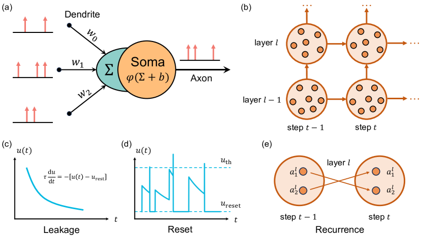
Figure 1: Illustration of the LIF-based spiking neuron model: (a) spike integration, transformation, and generation in a spiking neuron; (b) network structure of SNNs highlighting temporal and spatial dimensions; (c) leakage component reflecting membrane potential decaying; (d) reset component reflecting the membrane potential reset after each spike; (e) recurrence reflecting cross-neuron influence in the temporal dimension.

The LIF neuron model is governed by two main parts: the membrane potential dynamics and the spike generation mechanism. The membrane potential $u(t)$ can be described by the following differential equation:

$$\tau\frac{du}{dt}=-[u(t)-u_{\text{rest}}]+RI(t),$$ (1)

where $\tau$ is the membrane time constant, $u_{\text{rest}}$ is the resting membrane potential, $R$ is the membrane resistance, and $I(t)$ represents the input current. When the membrane potential exceeds a certain threshold value $u_{th}$, the neuron would fire a spike, and the membrane potential is reset to $u_{\text{reset}}$. This process can be formulated as

$$\begin{cases}o(t)=1~{}\&~{}u(t)=u_{reset},&\text{ if }u(t)\geq u_{th}\\ o(t)=0,&\text{ if }u(t)<u_{th}\end{cases}$$ (2)

where $o(t)$ represents the output spike at the $t$-th time step.

The continuous LIF model can be discretized using the Euler method, yielding the following iterative LIF model like

$$\begin{cases}u_{i}^{t,n}&=k_{\tau}u_{i}^{t-1,n}\left(1-o_{i}^{t-1,n}\right)+\sum_{j}w_{ij}^{n}o_{j}^{t,n-1},\\ o_{i}^{t,n}&=H\left(u_{i}^{t,n}-u_{th}\right),\end{cases}$$ (3)

where $u_{i}^{t,n}$ is updated at each time step in the $n$-th layer based on its previous state and the current input spikes. The synaptic weight connecting neurons $i$ and $j$ is denoted by $w_{ij}^{n}$, and $o_{i}^{t,n}$ represents the output spike of neuron $i$ at the $t$-th time step. The model also incorporates a leakage coefficient, $k_{\tau}$, to simulate the gradual decaying effect of the membrane potential over time, and a threshold potential, $u_{th}$, to control whether the neuron fires a spike. $H(\cdot)$ denotes the classic Heaviside function.

2.2 LIF Modelling Components

2.2.1 Leakage Component.

$k_{\tau}$ represents the leakage coefficient ranging within $[0,~{}1]$, which determines how fast the membrane potential $u$ decays over time. This component is responsible for the “leaky” functionality of the LIF neuron model, as it simulates the passive decay effect of the membrane potential.

2.2.2 Reset Component.

The output spike $o$ reflects the firing mechanism of the membrane potential and $(1-o)$ is responsible for resetting the membrane potential once the neuron fires. When the neuron fires (i.e., $o=1$), the reset mechanism resets the membrane potential by multiplying it by zero (i.e., $(1-o)=0$) in updating the membrane potential at the next time step. Otherwise, the membrane potential will remain unchanged. This component returns the membrane potential to a reset state after each spike event.

2.2.3 Recurrence Component.

This component is not presented in the equations above but can be added as recurrent connections at the network level. When included, the membrane potential dynamics can be rewritten as

$$u_{i}^{t,n}=k_{\tau}u_{i}^{t-1,n}\left(1-o_{i}^{t-1,n}\right)+\sum_{j}v_{ij}^{n}o_{j}^{t-1,n}+\sum_{j}w_{ij}^{n}o_{j}^{t,n-1}$$ (4)

where $v_{ij}^{n}$ represents the strength of the recurrent connection (synaptic weight) from neuron $j$ to neuron $i$ in the $n$-th layer. $o_{j}^{t-1,n}$ represents the spike state of neuron $j$ at the $(t-1)$-th time step. The recurrence component essentially provides feedback signals from the previous time step, allowing neurons to take the historic spike states of other neurons in the same layer into account when updating their membrane potentials.

3 Approach

In this section, we design several variant models with different component combinations as shown in Figure 2, allowing us to investigate the functional roles of different modelling components in LIF-based SNNs.

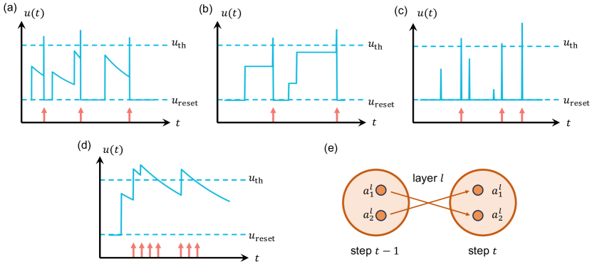
Figure 2: Variant models of LIF-based SNNs: (a) vanilla LIF; (b) without leakage; (c) complete leakage; (d) without reset; (e) with recurrence.

3.1 Different Leakage Coefficients.

The leakage component determines the decaying rate of the neuron’s membrane potential. This is an essential property of LIF neurons, as it can prevent the membrane potential from accumulating indefinitely. We design three variants as follows for considering this component.

Normal leakage. In this case, the membrane potential decays with a normal rate:

$$u_{i}^{t,n}=k_{\tau}u_{i}^{t-1,n}\left(1-o_{i}^{t-1,n}\right)+\sum_{j}w_{ij}^{n}o_{j}^{t,n-1},$$ (5)

which represents a balance between the cases without and complete leakage. This setting follows the vanilla LIF model with better bio-plausibility. Here we usually set $k_{\tau}=0.3$ for a typical value.

Without leakage. In this variant, the leakage coefficient is set to one:

$$u_{i}^{t,n}=1\cdot u_{i}^{t-1,n}\left(1-o_{i}^{t-1,n}\right)+\sum_{j}w_{ij}^{n}o_{j}^{t,n-1},$$ (6)

which means that the membrane potential does not decay at all. This results in full integration of current input signals and the previous membrane potential, allowing the neuron to accumulate inputs indefinitely.

Complete leakage. In this variant, the leakage coefficient is set to zero:

$$u_{i}^{t,n}=0\cdot u_{i}^{t-1,n}\left(1-o_{i}^{t-1,n}\right)+\sum_{j}w_{ij}^{n}o_{j}^{t,n-1}=\sum_{j}w_{ij}^{n}o_{j}^{t,n-1},$$ (7)

which means that the membrane potential decays completely at each single time step and is only determined by the current inputs.

3.2 Different Reset Modes.

The reset component is responsible for resetting the membrane potential of the neuron every time it fires, which prevents the neuron from firing continuously with a large potential value. We design two variants as follows for considering this component.

Normal reset. In this case, the reset term is included in the equation:

$$u_{i}^{t,n}=k_{\tau}u_{i}^{t-1,n}\left(1-o_{i}^{t-1,n}\right)+\sum_{j}w_{ij}^{n}o_{j}^{t,n-1}.$$ (8)

This reset term ensures that the neuron’s membrane potential will be reset to a lower state if the neuron fired in the last time step, i.e., $o_{i}^{t-1,n}=1$.

Without reset. In this variant, the reset term is removed from the equation:

$$u_{i}^{t,n}=k_{\tau}u_{i}^{t-1,n}+\sum_{j}w_{ij}^{n}o_{j}^{t,n-1}.$$ (9)

Consequently, the membrane potential will not be reset after it fires, allowing the neuron to continuously fire once its membrane potential reaches the threshold. This can lead to different dynamical properties and firing rates of the network.

3.3 Different Recurrence Patterns.

The recurrence component introduces recurrent connections within the network, allowing neurons to influence each other’s states. We design two variants as follows for considering this component.

Without recurrence. In this case, there are no recurrent connections between neurons:

$$u_{i}^{t,n}=k_{\tau}u_{i}^{t-1,n}\left(1-o_{i}^{t-1,n}\right)+\sum_{j}w_{ij}^{n}o_{j}^{t,n-1}.$$ (10)

The network is fully feedforward, and the output of one neuron does not influence the states of other neurons within the same layer at different time steps.

With recurrence. In this variant, recurrent connections between neurons are introduced into the network, as specified by the $\sum_{j}\mathrm{v}_{ij}^{n}o_{j}^{t-1,n}$ term:

$$u_{i}^{t,n}=k_{\tau}u_{i}^{t-1,n}\left(1-o_{i}^{t-1,n}\right)+\sum_{j}w_{ij}^{n}o_{j}^{t,n-1}+\sum_{j}\mathrm{v}_{ij}^{n}o_{j}^{t-1,n}.$$ (11)

This allows neurons to influence each other’s states in a feedback loop, leading to more complex dynamics and better learning of temporal features.

4 Experiments

This section offers an in-depth exploration of the functional roles of modelling components in LIF-based SNNs through a series of evaluation experiments, aiming at understanding how leakage, reset, and recurrence mechanisms impact the model performance. We initially focus on investigating the functional roles of three core components on different types of benchmarks. Our findings indicate that the impacts of these components can vary significantly on different datasets. Then, we further explore the generalization and robustness of SNNs. The generalization experiments focus on the adaptability of SNNs to different types of unseen data, with a particular emphasis on the neuromorphic datasets collected by DVS. In addition, the robustness assessment concentrates on the SNNs’ ability to resist adversarial attacks, serving as a complementary confirmation of the generalization capability. These comprehensive experiments help deepen our understanding of how SNNs work, paving the way for future development of neuromorphic models.

4.1 Accuracy Analysis on Different Benchmarks

4.1.1 Selection of Benchmarks.

In order to evaluate the performance of SNNs extensively, particularly focusing on the model variants of LIF-based SNNs, we select a range of benchmarks. These benchmarks are selected for their diversity and complexity, which enable a comprehensive assessment of different modelling components of SNNs and their functional roles.

Delayed Spiking XOR Problem. The delayed spiking XOR problem is customized to test the long-term memory capabilities of different neural network models [23]. This problem is structured in three stages: initially, an input spike pattern with a varying firing rate is injected into the network; then, it is followed by a prolonged delay period filled with noisy spikes; finally, the network receives another spike pattern and the network is expected to output the result of an XOR operation between the initial and final input spike patterns. The XOR operation is a concept in digital circuits, whose input and output signals only have binary states, one or zero. In the delayed spiking XOR problem, we correspond the high-firing-rate and low-firing-rate spike patterns to one and zero, respectively. This benchmark is crucial for understanding how different models memorize long-term information, particularly in scenarios where there is a long-term period filled with irrelevant data between two critical pieces of information.

Temporal Datasets. For temporal datasets, we select two speech signal datasets, SHD and SSC [24], listed in Table 1, as they provide rich temporal information that can test the capability of SNNs in processing temporal dependencies.

Table 1: Information of temporal datasets.

Attribute	SHD	SSC
Recordings	10,420	105,829
Classes	10	35
Type	Audio, spiking data	Audio, spiking data
Source	Microphone array	Microphone array
Format	Spike times	Spike times

Spatial Datasets. For the assessment of SNNs in handling spatial information, we select datasets listed in Table 2 whose data are distributed spatially in nature. This includes the MNIST dataset [25], famous for its collection of grayscale images of handwritten digits, and the CIFAR10 dataset [26], which presents a more complex set of color images depicting various natural scenes and objects. These spatial datasets are crucial to understand how SNNs can perform in recognizing spatial features.

Table 2: Information of spatial datasets.

Attribute	MNIST	CIFAR10
Images	70,000	60,000
Classes	10	10
Size	28x28 pixels	32x32 pixels
Source	Handwritten digits	Natural images
Format	Grayscale	RGB

Spatio-Temporal Datasets. To bridge the gap between purely temporal and spatial datasets, we additionally select datasets collected by DVS cameras, including Neuromorphic-MNIST (N-MNIST) [27] and DVS128 Gesture [12], listed in Table 3. DVS can capture visual information in a dynamic and event-driven manner, offering a blend of information in both spatial and temporal dimensions. The N-MNIST dataset, a neuromorphic adaptation of the spatial MNIST dataset, presents handwritten digits in a sequential temporal format. The DVS128 Gesture dataset, conversely, comprises recordings of various hand gestures, showcasing complex spatio-temporal patterns. These datasets provide a way to evaluate the capability of SNNs in handling spatio-temporal features simultaneously, making them ideal for understanding the functional roles of their modelling components. For the N-MNIST dataset, we use a fixed time interval to integrate events as frames for post-processing with a limited number of time steps. However, for the DVS128 Gesture dataset, due to the variation in sample durations, we adopt a fixed-frame compression method to ensure that all samples are of uniform length [28, 29].

Table 3: Information of spatio-temporal datasets.

Attribute	N-MNIST	DVS128 Gesture
Samples	70,000	1,342
Classes	10	11
Size	34x34 pixels	128x128 pixels
Source	Neuromorphic handwritten digits	Dynamic hand gestures
Format	DVS format	DVS format

4.1.2 Experimental Setup.

We implement the LIF neuron model with different configurations for each of the three modelling components: leakage, reset, and recurrence. The performance of all variant models is evaluated on selected benchmarks. We employ similar network structures and hyper-parameter configurations for different variant models to provide a fair comparison. All networks are trained with backpropagation through time (BPTT)[30, 31], in which surrogate gradients are used to solve the nondifferentiability of spike activities. The detailed network architectures for each dataset are provided in Table 4. Note that the complexity of CIFAR10 makes it challenging for Multi-Layer Perceptrons (MLPs). To overcome this issue, we employ SNNs with convolutional layers. Therefore, experiments with recurrence are omitted for CIFAR10, given the inconvenience in adding recurrent connections onto convolutional architectures[32, 3].

Table 4: Network structures for different models and datasets.

Dataset	Network structures
SHD	Input(700)–$\textnormal{FC}_{LIF}$(64)-$\textnormal{FC}_{LIF}$(20)-Output
SSC	Input(700)–$\textnormal{FC}_{LIF}$(200)-$\textnormal{FC}_{LIF}$(35)-Output
N-MNIST	Input(2312)–$\textnormal{FC}_{LIF}$(512)-$\textnormal{FC}_{LIF}$(10)-Output
DVS128 Gesture	Input(32768)–Downsampling(2048)–$\textnormal{FC}_{LIF}$(512)-$\textnormal{FC}_{LIF}$(512)-$\textnormal{FC}_{LIF}$(11)-Output
MNIST	Input(784)–$\textnormal{FC}_{LIF}$(512)-$\textnormal{FC}_{LIF}$(10)-Output
CIFAR10	Input(3072)–$\textnormal{ResNet18}_{LIF}$-Output

We adopt a uniform set of hyper-parameters for different models, ensuring a fair comparison between variant models. These hyper-parameters include the number of epochs, batch size, learning rate, and SNN-specific parameters like the firing threshold and the gradient width during backpropagation. The Adam optimizer is employed for all models, with a learning rate scheduler to adjust the learning rate during training. The detailed hyper-parameter settings can be found in Table 5, enabling a consistent and reproducible experimental setup.

Table 5: Hyper-parameter settings for different models and datasets.

Parameter	Temporal Datasets	Spatio-temporal Datasets	Spatial Datasets
#Epochs	100	100	100
Batch Size	512	1024	512
Learning Rate	1e-2	1e-4	1e-4
$u_{th}$	0.5	0.3	0.3
Surrogate Gradient Width	0.5	0.25	0.25
Optimizer	Adam	Adam	Adam
Scheduler	StepLR (20, 0.5)	StepLR (25, 0.1)	StepLR (25, 0.1)

Specifically, for temporal datasets where temporal dependencies are quite hard to learn, we adopt a learnable leakage in the baseline for better accuracy. In contrast, for spatio-temporal and spatial datasets, we maintain a fixed leakage across all experiments. In all experiments, each variant model alters only one component at a time, ensuring that the observed effects can be attributed solely to the change of the specific component.

4.1.3 Results and Analyses.

As reflected in Table 6 and Figure 3, we observe that the influence of the three modelling components of SNNs, leakage, reset, and recurrence, varies significantly on different types of benchmarks. Notably, the impact is most significant on the temporal benchmarks, followed by the spatio-temporal datasets, with the least influence observed on spatial datasets. This trend aligns with reasonable expectations considering the nature of these benchmarks. Temporal ones inherently involve dynamic dependencies over time, thereby highlighting the effects of these components more distinctly in adapting the membrane potential dynamics. Spatio-temporal datasets with hybridization of temporal dynamics and spatial features, exhibit a moderate level of influence. In contrast, spatial datasets, which primarily focus on static spatial features, show the least sensitivity to these variations in component combinations. Therefore, we recommend using the results on temporal datasets for in-depth analyses to avoid misleading in this part.

Table 6: Accuracy comparison between variant models on different benchmarks.

	Temporal				Spatio-Temporal			Spatial
Dataset	XOR	SHD	SSC		N-MNIST	DVS128 Gesture		MNIST	CIFAR10
Baseline	77.50%	78.58%	60.70%		94.76%	86.81%		95.22%	92.25%
Without leakage	50.30%	66.12%	44.44%		95.18%	87.50%		96.12%	92.67%
Complete leakage	50.50%	5.96%	3.22%		95.03%	86.11%		94.17%	92.28%
Without reset	96.10%	78.89%	60.70%		96.18%	87.84%		94.85%	93.29%
With recurrence	98.90%	80.43%	66.53%		96.21%	89.93%		96.98%	–

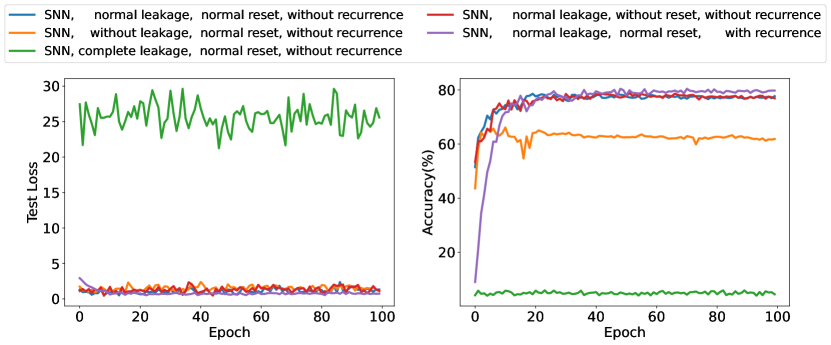
Figure 3: Loss and accuracy curves of variant models on SHD.

The role of the leakage. The leakage coefficient directly determines the decaying rate of the membrane potential over time. In processing long temporal sequences, the decaying rate of the membrane potential plays a crucial role in a model’s ability to learn long-term dependencies. A higher leakage rate (i.e., smaller $k_{\tau}$) tends to make it difficult for the model to retain and utilize information over a long period.

Specifically, when a model is set with a complete leakage (i.e., $k_{\tau}=0$), it totally fails to retain any information from previous time steps. This complete leakage results in quite low accuracy especially on the temporal benchmarks, where a model with complete leakage struggles to perform better than just random guessing in classification. On the other hand, when the setting is without leakage (i.e., $k_{\tau}=1$) also degrade the accuracy compared to the learnable leakage coefficient. The leakage coefficient is intrinsically linked to the signal frequency that the model can respond well to. A lower leakage corresponds to slower response and longer signal cycles. Therefore, the setting without leakage would impair the model’s response capability to high-frequency signals, leading to decreased accuracy.

The role of the reset mode. The reset mechanism of the LIF neuron model serves as another critical role in learning temporal dynamics. When the membrane potential surpasses a certain threshold, the neuron fires a spike, and the reset mechanism subsequently reinitializes the membrane potential to a lower value. While this mechanism aligns with biological plausibility and aims to prevent unbounded potential accumulation, it inadvertently disrupts the temporal continuity that matters in performing certain tasks.

Specifically, in the delayed spiking XOR problem, the reset mechanism in the baseline model shows a significant degradation in accuracy. The reset process erases the membrane potential completely, cleaning all historic information, which makes it failed to memorize long-term dependencies in this task. This effect is weakened on spatio-temporal and purely spatial benchmarks due to the poorer temporal information. Notice that the impact of the reset mechanism is smaller than that of the leakage component on SHD and SSD datasets with higher complexity, therefore the observed differences are not significant.

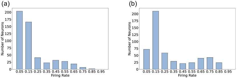
Figure 4: Average spike rate distribution of variant models on N-MNIST: (a) normal reset; (b) without reset.

In addition, the reset mechanism greatly impacts the firing rate of neurons. As illustrated in Figure 4, the reset can reduce the firing rate by returning the membrane potential to a lower value every time a spike fires. This action leads to sparser spike activities, which is advantageous for higher computational efficiency [33, 34]. Such a feature is particularly beneficial in edge computing devices, where computational resources and power supply are limited.

The role of the recurrence pattern. The incorporation of the recurrence component in SNNs endows these models with the capability to exchange information between different neurons in the same layer across time steps. This cross-neuron information fusion significantly enhances the model’s capability in learning, capturing, and integrating temporal features. In temporal computing tasks, the presence of recurrence generally results in superior accuracy. Similarly, the improvement would decrease when the benchmarks have fewer temporal dependencies such as on spatial benchmarks.

4.2 Generalization Analyses on Spatio-Temporal datasets

Generalization is pivotal in understanding the model’s capacity to adapt to unseen data and really matters in real-world applications. Recent studies investigating the generalization capability of SNNs have unveiled noteworthy results, especially in comparison to RNNs [13]. In this section, we present a series of experiments on the spatio-temporal datasets collected by DVS, to evaluate the generalization of variant models and analyze the underlying mechanisms. We delve into this phenomenon from two perspectives: the relationship between the flatness of the loss landscapes and the generalization in machine learning theory; the impact of different modelling components of SNNs on error accumulation and gradient backpropagation.

4.2.1 Experimental Setup

DVS cameras represent an emerging imaging technology that capture pixel-level changes in luminance, resulting in asynchronous, event-driven, sparse, and temporal event streams. One of the prominent datasets collected by DVS is the N-MNIST dataset, a neuromorphic version of the classic MNIST dataset. It is generated by moving the MNIST images in front of a DVS camera that records the spike outputs, thus converting static images into temporal event streams and offering richer temporal information.

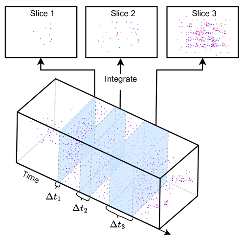
Figure 5: Spatio-temporal data collected by DVS with variable temporal integration lengths.

We process the N-MNIST dataset with varying temporal integration lengths to generate different frame-like sequence datasets. As shown in Figure 5, this approach generates multiple datasets, each of which is characterized by a specific temporal resolution determined by the temporal integration length, thereby enabling a comprehensive assessment of the generalization capability of SNNs. In our experiments, the N-MNIST event streams are integrated over different temporal integration lengths (i.e., 1$ms$, 2$ms$, 3$ms$, 5$ms$, and 10$ms$) to create varying temporal resolutions. The primary training is conducted on the 3$ms$ configuration, and the network structures and hyper-parameter settings are consistent with those mentioned in Table 4 and Table 5 for the N-MNIST dataset. The corresponding RNN network structure is “Input(2312)–RNN(512)–FC(10)–Output”, including Vanilla RNNs, Long Short-Term Memory (LSTM) [35] networks, and Gated Recurrent Units (GRU) [36]. After pre-training, subsequent testing is performed on datasets with different temporal integration lengths (i.e., 1$ms$, 2$ms$, 5$ms$, and 10$ms$) to evaluate the model’s generalization capability by examining the testing accuracy.

4.2.2 Results.

Table 7: Generalization comparison between models under variable timescales.

	Components				Temporal Resolution
Model	Leakage	Reset	Recurrence		1$ms$	2$ms$	3$ms$	5$ms$	10$ms$
SNN (Baseline)	Normal	Normal	Without		90.82%	94.14%	94.76%	94.80%	94.63%
SNN	Without	Normal	Without		88.70%	94.49%	95.18%	95.26%	95.07%
SNN	Complete	Normal	Without		90.98%	94.57%	95.03%	95.12%	95.14%
SNN	Normal	Without	Without		93.90%	95.83%	96.18%	96.30%	96.12%
SNN	Normal	Normal	With		75.51%	93.72%	96.21%	94.00%	80.41%
SNN	Without	Normal	With		59.14%	93.48%	96.48%	92.57%	70.11%
SNN	Without	Without	With		36.92%	89.16%	93.40%	90.91%	74.01%
LSTM	-	-	-		31.62%	90.52%	97.84%	63.10%	9.84%
GRU	-	-	-		23.25%	77.69%	96.88%	81.83%	45.20%
Vanilla RNN	-	-	-		17.68%	18.28%	93.84%	37.58%	19.92%

As reflected in Table 7, an intuitive observation indicates a significant superiority in generalization performance for SNNs compared to all RNN models. In the spectrum of variant SNNs, it is noted that the absence of leakage leads to a decline in generalization, particularly evident under the 1$ms$ temporal resolution. Furthermore, the incorporation of recurrence seems to impair the generalization capability notably. When combining the worst setting without leakage, without reset, and with recurrence in an SNN model, the generalization capability significantly drops, approaching the level observed in the LSTM model. It seems that the impact of the reset is more subtle compared to those of the leakage and recurrence, but helpful when the model accuracy is low for example comparing the settings without leakage, normal/without reset, and with recurrence.

4.2.3 Comparing Loss Landscapes.

The concept of loss landscape flatness is an important concept for understanding the generalization capability of a neural network. Flat regions in the loss landscape indicate where small variations of the network parameters result in minor changes of the loss value [37]. In contrast, steep regions represent sensitive areas where minor parameter changes can lead to significant loss alterations. Therefore, a flatter minima in the loss landscape implies that noises and shifts in the data distribution will not lead to significant loss increases, ensuring more stable performance for unseen data.

We adopt the method introduced by Li et al. [38] to visualize the loss landscape of neural networks. This approach allows to visualize the high-dimensional loss landscape by projecting it onto a two-dimensional space. The key concept is to plot the network’s loss with respect to random directions in the parameter space. This visualization technique provides an intuitive understanding of the optimization landscape, highlighting areas with a flat minima for better generalization.

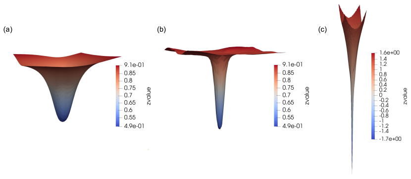
Figure 6: Comparison of the loss landscapes: (a) vanilla SNN; (b) variant SNN without leakage and with recurrence; (c) LSTM.

We visualize three models: a vanilla SNN, a variant SNN without leakage and with recurrence, and an LSTM model, whose network structures and hyper-parameter settings are consistent with those described in Table 4 and Table 5 for the N-MNIST dataset. As presented in Figure 6, the loss landscape visualization reveals that the vanilla SNN exhibits the flattest optimization landscape, followed by the variant SNN, while the LSTM shows the steepest landscape. This suggests that SNNs inherently possess better generalization. It might be attributed to their spike-based neuronal dynamics with a discrete state space and automatic membrane potential decaying that can resist perturbations to a great extent. It can be seen that removing the leakage that prevents the membrane potential from decaying and introducing recurrence that increases the probability of state transfer in the state space, would harm the generalization capability. The flat loss landscape observed in SNNs implies that they have a higher tolerance to parameter or input perturbations, which can be advantageous in dynamic and noisy environments. With above observations, we further analyze the impacts of individual modelling components of SNNs on the generalization capability in the following parts.

The role of the leakage. In vanilla SNNs, leakage refers to the gradual decay of the membrane potential over time, preventing indefinite accumulation of the membrane potential error. Removing the leakage would magnify the impact of errors, especially in networks with long time steps or deep layers. In the context of BPTT, this can be illustrated by considering the gradient of the loss function with respect to the membrane potential at a given time step $t$, denoted as $\frac{\partial L}{\partial u(t)}$. In the variant without leakage, the gradient can be expanded as

$$\frac{\partial L}{\partial u(t)}=\frac{\partial L}{\partial o(t)}\cdot\frac{\partial o(t)}{\partial u(t)}+\frac{\partial L}{\partial u(t+1)}\cdot\frac{\partial u(t+1)}{\partial u(t)}.$$ (12)

Note that $\frac{\partial u(t+1)}{\partial u(t)}$ can be significantly impacted by the absence of leakage. Typically, a leakage coefficient $k_{\tau}$ would scale down $\frac{\partial u(t+1)}{\partial u(t)}$, reducing the propagated error. Without this scaling after removing the leakage, errors propagate fast, affecting the learning stability and generalization.

The role of the reset mode. The reset mechanism, which only occurs at the firing time step, has a lower impact on the error accumulation. Although the reset mechanism induces a discontinuity in the membrane potential, this effect does not inherently contribute a lot to the error propagation over multiple time steps. However, it’s important to note that when combining the setting without reset to the setting without leakage and with recurrence, the generalization capability notably drops. This suggests that while the individual effect of the reset mode might be limited, its interaction with other components can lead to significant influences.

The role of the recurrence pattern. Recurrence in SNNs, introducing cross-neuron dynamics over time steps, allow these errors to propagate more broadly across the network. This exacerbates the error propagation, significantly impacting the generalization capability. This effect is especially pronounced when combining the absence of leakage together, where the errors from previous time steps are not attenuated.

The recurrence mechanism can be formalized as

$$u(t)=f(\sum_{j}v_{ij}^{n}o_{j}^{t-1,n},\ldots),$$ (13)

where $f$ represents the update function incorporating recurrent inputs. The gradient $\frac{\partial L}{\partial u(t)}$ in this situation becomes more complex due to the additional terms involving past outputs of other neurons. This complexity magnifies the error accumulation, leading to more significant degradation of generalization.

4.2.4 Feature Space Analysis with t-SNE Visualization.

We further visualize the feature representation learned by each variant SNN using t-SNE dimensionality reduction [39, 40]. This technique allows us to visualize the high-dimensional features from the last hidden layer in a two-dimensional space, providing an intuitive understanding of how different components influence the feature space.

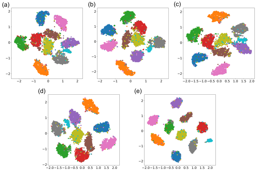
Figure 7: Feature visualization of the last hidden layer of variant models: (a) vanilla SNN; (b) without leakage; (c) complete leakage; (d) without reset; (e) with recurrence.

As illustrated in Figure 7, the variant SNN with recurrence demonstrates the most distinctive class separation, followed by closer class distributions observed in the remaining variants. This observation aligns with previous findings that the setting with recurrence can enrich the model’s capability to capture complex temporal dynamics, resulting in more distinctive feature representation and higher accuracy. However, this leads to a steeper loss landscape with poorer generalization, which is usually ignored by most works focusing on the accuracy result.

4.2.5 Comparison to RNNs.

RNNs, with natural recurrence, face challenges in handling long sequences, primarily due to gradient vanishing or exploding. Unlike the vanilla RNN, LSTM and GRU typically include multiple state paths and gating mechanisms to mitigate this issue. Specifically, LSTM provides a more effective control over the information flow through two state variables and four gates, which allows to retain or forget information flexibly across long sequences. GRU further simplifies the architecture by using only two gates and merging the cell and hidden states. In a nutshell, their different architectures result in a performance priority following LSTMs, GRUs, and vanilla RNNs. SNNs remain the multiple state paths, membrane potential and spike event, which behave like LSTMs with great potential in learning long sequences. Furthermore, SNNs simplify the complex gate structures but introduce leakage, firing, and reset mechanisms that endow them enhanced generalization.

4.3 Robustness against Adversarial Attack

Adversarial attacks produce a significant challenge for neural networks, especially in applications where security and reliability are critical [41]. These attacks are characterized by malicious input perturbations that mislead neural networks to incorrect classifications or predictions. In this context, SNNs have attracted attention for robust intelligence due to their unique temporal dynamics and modelling components, which are distinct from conventional ANNs. Investigating the robustness of SNNs is not only academically fascinating but also holds substantial practical value in developing more secure intelligent systems.

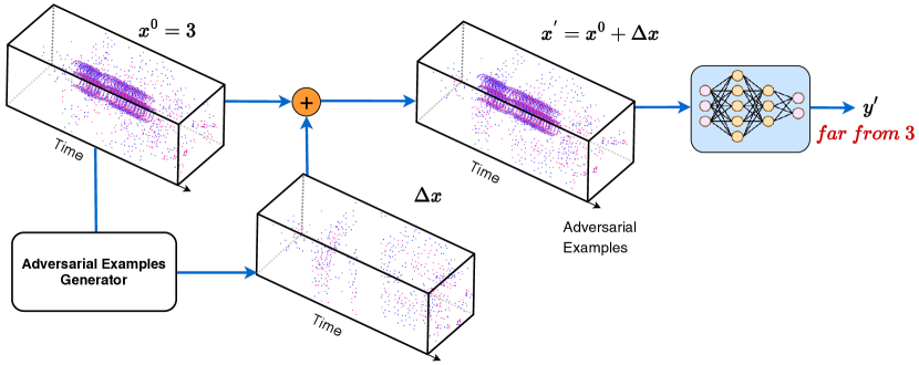
Figure 8: Workflow of the adversarial attack for SNNs.

4.3.1 Experimental Setup.

Inspired by the approach in Liang et al. [14], we generate adversarial examples for SNNs following the workflow in Figure 8. The attack involves perturbing the input spikes in a way that causes misclassification while ensuring that the perturbations are minimal and indiscernible to human observers. Network structures and hyper-parameter settings are consistent with those described in Table 4 and Table 5 for the N-MNIST dataset. The primary metric for evaluating adversarial robustness is the attack success rate, which measures the proportion of adversarial examples that can lead to misclassification successfully. Furthermore, the model robustness can be quantified by the average perturbation magnitude required to induce misclassification. To establish a more fair comparison of robustness, we fix the attack success rate at 100% and then compare the average perturbation needed to reach such high attack success rate. A smaller perturbation implies lower robustness.

4.3.2 Results and Analysis.

The results obtained from the adversarial robustness experiments are presented in Figure 9. Among the variant SNNs, leakage and recurrence are the most influential factors that impact the adversarial robustness. As the leakage rate increases (i.e., smaller $k_{\tau}$), the robustness of SNNs against adversarial attacks can be improved; conversely, SNNs with reduced or without leakage exhibit a decline in robustness. This phenomenon can be attributed to the fact that a higher leakage rate prevents the error accumulation, thereby reducing the network’s susceptibility to small input perturbations. The introduction of recurrence tends to degrade the robustness. While the recurrent connections enrich the model’s capacity to process temporal data, they also introduce additional pathways for the error propagation, making recurrent SNNs more vulnerable to adversarial attacks. The influence of the reset component on adversarial robustness is less significant, suggesting that the reset mechanism, which primarily affects the network at the moment of spike generation, does not heavily impact the overall resistance to adversarial attacks.

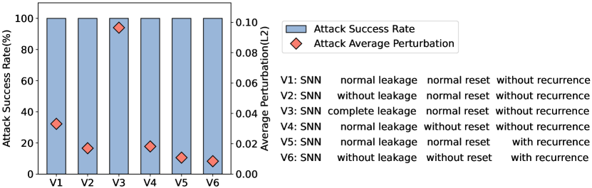
Figure 9: Comparing adversarial robustness between variant models.

Generalization experiments focus on testing the model performance on processing unseen data, while adversarial attack examines specific robustness of the model in resisting adversarial examples. Notably, the findings in adversarial attack experiments are consistent with those observed from the generalization experiments. This alignment further strengthens our understanding of the functional roles of SNN modelling components, paving the way for the development of more effective and robust neuromorphic models.

5 Optimization Suggestions

Based on the comprehensive experiments and analyses presented in previous sections, here we summarize several suggestions for optimizing SNNs in different tasks. These suggestions leverage our in-depth understanding of the functional roles of modelling components in the LIF-based SNNs.

Suggestions for temporal computing tasks. (1) For tasks that need a long-term memory, an elaborate leakage rate is critical. A high leakage rate (i.e., small $k_{\tau}$) cannot memorize temporal information for a long time, thus a lower leakage rate is recommended. Note that if the task is quite difficult, e.g., SHD and SSC datasets, a too low leakage rate cannot track the fast-changing signals closely, which can also degrade the performance. If so, a learnable parameter of the leakage coefficient is recommended. (2) For tasks that need continuous processing of temporal information without disruption such as the delayed spiking XOR problem, disabling the reset mechanism could be beneficial. However, the increase of the firing rate without reset would decrease the computational efficiency. (3) For tasks that model complex temporal dynamics, the incorporation of recurrence can enhance the representation ability. However, this might lead to overfitting, for which considering the trade-off between accuracy and generalization/robustness is necessary.

Suggestions for generalization and robustness. (1) For tasks where generalization and robustness are paramount, a higher leakage rate (i.e., smaller $k_{\tau}$) can enhance the resistance to input perturbations by reducing error accumulation. (2) For these tasks, avoiding recurrence, although beneficial for temporal processing, is helpful for improving model generalization and robustness due to the increasing error propagation paths. Note that the gain of higher generalization and robustness might harm the application accuracy, which again reflects the trade-off mentioned above.

6 Conclusion

This work systematically explores the functional roles of modelling components in LIF-based SNNs. With customized variant models and extensive comprehensive on diverse benchmarks, we get valuable observations on how the leakage, reset, and recurrence components influence the behaviors of SNNs. Finally, we provide suggestions for model optimization in different tasks. Specifically, the leakage component plays a crucial role in balancing memory retention and robustness. A lower leakage rate can enhance the memory capability of long-term dependencies, but makes the model sensible to noisy input perturbations due to the larger error accumulation. The reset component, while not impacting generalization and robustness significantly, sometimes degrades the application accuracy in tasks that need uninterrupted temporal processing and can be improved by disabling it for maintaining temporal continuity. The recurrence component allows to model complex temporal dynamics by introducing feedback connections, which can improve the application accuracy for complex temporal computing tasks. However, the recurrence increases the risks of worse generalization and robustness due to the cross-neuron error propagation paths. There findings deepen the understanding of SNNs and help identify the key modelling components for guiding the development of effective and robust neuromorphic models in different application scenarios.

References

References

- [1] Demis Hassabis, Dharshan Kumaran, Christopher Summerfield, and Matthew Botvinick. Neuroscience-inspired artificial intelligence. Neuron, 95(2):245–258, 2017.
- [2] Yann LeCun, Yoshua Bengio, and Geoffrey Hinton. Deep learning. nature, 521(7553):436–444, 2015.
- [3] Kaiming He, Xiangyu Zhang, Shaoqing Ren, and Jian Sun. Deep residual learning for image recognition. In Proceedings of the IEEE conference on computer vision and pattern recognition, pages 770–778, 2016.
- [4] Kai Sheng Tai, Richard Socher, and Christopher D Manning. Improved semantic representations from tree-structured long short-term memory networks. arXiv preprint arXiv:1503.00075, 2015.
- [5] Ashish Vaswani, Noam Shazeer, Niki Parmar, Jakob Uszkoreit, Llion Jones, Aidan N Gomez, Łukasz Kaiser, and Illia Polosukhin. Attention is all you need. Advances in neural information processing systems, 30, 2017.
- [6] Lei Deng, Yujie Wu, Xing Hu, Ling Liang, Yufei Ding, Guoqi Li, Guangshe Zhao, Peng Li, and Yuan Xie. Rethinking the performance comparison between snns and anns. Neural networks, 121:294–307, 2020.
- [7] Adam H Marblestone, Greg Wayne, and Konrad P Kording. Toward an integration of deep learning and neuroscience. Frontiers in computational neuroscience, 10:94, 2016.
- [8] Amirhossein Tavanaei, Masoud Ghodrati, Saeed Reza Kheradpisheh, Timothée Masquelier, and Anthony Maida. Deep learning in spiking neural networks. Neural networks, 111:47–63, 2019.
- [9] Wolfgang Maass. Networks of spiking neurons: the third generation of neural network models. Neural networks, 10(9):1659–1671, 1997.
- [10] Qiongyi Zhou, Changde Du, and Huiguang He. Exploring the brain-like properties of deep neural networks: a neural encoding perspective. Machine Intelligence Research, 19(5):439–455, 2022.
- [11] Bing Han and Kaushik Roy. Deep spiking neural network: Energy efficiency through time based coding. In European Conference on Computer Vision, pages 388–404. Springer, 2020.
- [12] Arnon Amir, Brian Taba, David Berg, Timothy Melano, Jeffrey McKinstry, Carmelo Di Nolfo, Tapan Nayak, Alexander Andreopoulos, Guillaume Garreau, Marcela Mendoza, et al. A low power, fully event-based gesture recognition system. In Proceedings of the IEEE conference on computer vision and pattern recognition, pages 7243–7252, 2017.
- [13] Weihua He, YuJie Wu, Lei Deng, Guoqi Li, Haoyu Wang, Yang Tian, Wei Ding, Wenhui Wang, and Yuan Xie. Comparing snns and rnns on neuromorphic vision datasets: Similarities and differences. Neural Networks, 132:108–120, 2020.
- [14] Ling Liang, Xing Hu, Lei Deng, Yujie Wu, Guoqi Li, Yufei Ding, Peng Li, and Yuan Xie. Exploring adversarial attack in spiking neural networks with spike-compatible gradient. IEEE transactions on neural networks and learning systems, 2021.
- [15] Ling Liang, Zheng Qu, Zhaodong Chen, Fengbin Tu, Yujie Wu, Lei Deng, Guoqi Li, Peng Li, and Yuan Xie. H2learn: High-efficiency learning accelerator for high-accuracy spiking neural networks. IEEE Transactions on Computer-Aided Design of Integrated Circuits and Systems, 41(11):4782–4796, 2021.
- [16] Guillaume Bellec, Darjan Salaj, Anand Subramoney, Robert Legenstein, and Wolfgang Maass. Long short-term memory and learning-to-learn in networks of spiking neurons. Advances in neural information processing systems, 31, 2018.
- [17] Eugene M Izhikevich. Simple model of spiking neurons. IEEE Transactions on neural networks, 14(6):1569–1572, 2003.
- [18] Wulfram Gerstner, Werner M Kistler, Richard Naud, and Liam Paninski. Neuronal dynamics: From single neurons to networks and models of cognition. Cambridge University Press, 2014.
- [19] Mohamed Sadek Bouanane, Dalila Cherifi, Elisabetta Chicca, and Lyes Khacef. Impact of spiking neurons leakages and network recurrences on event-based spatio-temporal pattern recognition. arXiv preprint arXiv:2211.07761, 2022.
- [20] Sayeed Shafayet Chowdhury, Chankyu Lee, and Kaushik Roy. Towards understanding the effect of leak in spiking neural networks. Neurocomputing, 464:83–94, 2021.
- [21] Xingting Yao, Fanrong Li, Zitao Mo, and Jian Cheng. Glif: A unified gated leaky integrate-and-fire neuron for spiking neural networks. Advances in Neural Information Processing Systems, 35:32160–32171, 2022.
- [22] Wachirawit Ponghiran and Kaushik Roy. Spiking neural networks with improved inherent recurrence dynamics for sequential learning. In Proceedings of the AAAI Conference on Artificial Intelligence, volume 36, pages 8001–8008, 2022.
- [23] Hanle Zheng, Zhong Zheng, Rui Hu, Bo Xiao, Yujie Wu, Xue Liu, Guoqi Li, and Lei Deng. Temporal dendritic heterogeneity incorporated with spiking neural networks for learning multi-timescale dynamics. Nature Communications, 2024 (In Press).
- [24] Benjamin Cramer, Yannik Stradmann, Johannes Schemmel, and Friedemann Zenke. The heidelberg spiking data sets for the systematic evaluation of spiking neural networks. IEEE Transactions on Neural Networks and Learning Systems, 33(7):2744–2757, 2020.
- [25] Yann LeCun, Léon Bottou, Yoshua Bengio, and Patrick Haffner. Gradient-based learning applied to document recognition. Proceedings of the IEEE, 86(11):2278–2324, 1998.
- [26] Alex Krizhevsky, Geoffrey Hinton, et al. Learning multiple layers of features from tiny images. Toronto, ON, Canada, 2009.
- [27] Garrick Orchard, Ajinkya Jayawant, Gregory K Cohen, and Nitish Thakor. Converting static image datasets to spiking neuromorphic datasets using saccades. Frontiers in neuroscience, 9:437, 2015.
- [28] Wei Fang, Zhaofei Yu, Yanqi Chen, Timothée Masquelier, Tiejun Huang, and Yonghong Tian. Incorporating learnable membrane time constant to enhance learning of spiking neural networks. In Proceedings of the IEEE/CVF international conference on computer vision, pages 2661–2671, 2021.
- [29] Wei Fang, Yanqi Chen, Jianhao Ding, Zhaofei Yu, Timothée Masquelier, Ding Chen, Liwei Huang, Huihui Zhou, Guoqi Li, and Yonghong Tian. Spikingjelly: An open-source machine learning infrastructure platform for spike-based intelligence. Science Advances, 9(40):eadi1480, 2023.
- [30] Yujie Wu, Lei Deng, Guoqi Li, Jun Zhu, and Luping Shi. Spatio-temporal backpropagation for training high-performance spiking neural networks. Frontiers in neuroscience, 12:331, 2018.
- [31] Yujie Wu, Lei Deng, Guoqi Li, Jun Zhu, Yuan Xie, and Luping Shi. Direct training for spiking neural networks: Faster, larger, better. In Proceedings of the AAAI conference on artificial intelligence, volume 33, pages 1311–1318, 2019.
- [32] Yann LeCun, Yoshua Bengio, et al. Convolutional networks for images, speech, and time series. The handbook of brain theory and neural networks, 3361(10):1995, 1995.
- [33] Lei Deng, Guoqi Li, Song Han, Luping Shi, and Yuan Xie. Model compression and hardware acceleration for neural networks: A comprehensive survey. Proceedings of the IEEE, 108(4):485–532, 2020.
- [34] Lei Deng, Yujie Wu, Yifan Hu, Ling Liang, Guoqi Li, Xing Hu, Yufei Ding, Peng Li, and Yuan Xie. Comprehensive snn compression using admm optimization and activity regularization. IEEE transactions on neural networks and learning systems, 2021.
- [35] Sepp Hochreiter and Jürgen Schmidhuber. Long short-term memory. Neural computation, 9(8):1735–1780, 1997.
- [36] Kyunghyun Cho, Bart Van Merriënboer, Caglar Gulcehre, Dzmitry Bahdanau, Fethi Bougares, Holger Schwenk, and Yoshua Bengio. Learning phrase representations using rnn encoder-decoder for statistical machine translation. arXiv preprint arXiv:1406.1078, 2014.
- [37] Yoshua Bengio. Practical recommendations for gradient-based training of deep architectures. In Neural Networks: Tricks of the Trade: Second Edition, pages 437–478. Springer, 2012.
- [38] Hao Li, Zheng Xu, Gavin Taylor, Christoph Studer, and Tom Goldstein. Visualizing the loss landscape of neural nets. Advances in neural information processing systems, 31, 2018.
- [39] Laurens Van der Maaten and Geoffrey Hinton. Visualizing data using t-sne. Journal of machine learning research, 9(11), 2008.
- [40] Martin Wattenberg, Fernanda Viégas, and Ian Johnson. How to use t-sne effectively. Distill, 1(10):e2, 2016.
- [41] Aleksander Madry, Aleksandar Makelov, Ludwig Schmidt, Dimitris Tsipras, and Adrian Vladu. Towards deep learning models resistant to adversarial attacks. arXiv preprint arXiv:1706.06083, 2017.