The Directionality of
Gravitational and Thermal Diffusive Transport
in Geologic Fluid Storage

Abstract

Diffusive transport has implications for the long-term status of underground storage of hydrogen (H₂) fuel and carbon dioxide (CO₂), technologies which are being pursued to mitigate climate change and advance the energy transition. Once injected underground, CO₂ and H₂ will exist in multiphase fluid-water-rock systems: being partially-soluble, injected fluids can flow through the porous rack in a connected plume, become disconnected and trapped as ganglia surrounded by groundwater within the storage rock pore space, and also dissolve and migrate through the aqueous phase once dissolved. Recent analyses have focused on the concentration gradients induced by differing capillary pressure between fluid ganglia which can drive diffusive transport (“Ostwald ripening”). However, studies have neglected or excessively simplified important factors; namely: the non-ideality of gases under geologic conditions, the opposing equilibrium state of dissolved CO₂ and H₂ driven by the partial molar density of dissolved solutes, and entropic and thermodiffusive effects resulting from geothermal gradients. We conduct an analysis from thermodynamic first principles and use this to provide numerical estimates for CO₂ and H₂ at conditions relevant to underground storage reservoirs. We show that while diffusive transport in isothermal systems is upwards for both gases, as indicated by previous analysis, entropic contributions to the free energy are so significant as to cause a reversal in the direction of diffusive transport in systems with geothermal gradients. For CO₂, even geothermal gradients less than 10^oC/km (far less than typical gradients of 25^oC/km) induce downwards diffusion at depths relevant to storage. Diffusive transport of H₂ is less affected, but still reverses direction under typical gradients, e.g. 30^oC/km, at a depth of 1000 m. The entropic contribution also modifies the magnitude of flux where geothermal gradients are present, with the largest diffusive fluxes estimated for CO₂ with a 30^oC/km gradient, despite the higher diffusion coefficient of H₂. We find a maximum flux on the order of 10^-13 for CO₂ in the 30^oC/km scenario, still four orders of magnitude smaller than literature estimates of density-driven convective flux. Contrary to previous studies, we find that in diffusion and convection will likely work in concert – both driving CO₂ downwards, and both driving H₂ upwards – for conditions representative of their respective storage reservoirs.

I Introduction

Geologic formations underground offer high capacity, potentially long-term storage options for fluids such as waste carbon dioxide (CO₂) and gaseous hydrogen fuel (H₂), offering significant potential to mitigate climate change, provide energy storage, and accelerate the energy transition away from fossil fuels [1, 2, 3, 4, 5, 6]. Saline reservoirs – porous host rock formations saturated with saline aqueous phase (“brine”) – comprise the largest resource of underground storage options [7]. Once injected into a saline reservoir underground, the partially soluble CO₂ or H₂ fluid (which will be referred to as ‘gas’ in this work to distinguish if from the aqueous fluid phase) will flow through the architecture of the porous host rock along with the brine, with configurations and flow properties dictated by the local (pore-scale) capillary behavior of the rock-brine-fluid multiphase system. Because CO₂ or H₂ are typically non-wetting relative to the aqueous liquid, much of the injected gas may become “snapped off” into small disconnected ganglia, and held by capillarity within pore bodies of the host rock [8]. This is known as residual trapping. From this point, the primary transport of the injected fluids will occur through the aqueous phase: advection with the aqueous flow field, convection due to density gradients (e.g. [9, 10]), and diffusion due to concentration, gravitational, and thermal gradients (e.g. [11]).

This work focuses on the diffusive transport processes and how these may manifest in a multiphase system where concentration gradients of dissolved gas are imposed due to the presence of these residually-trapped ganglia. For partially soluble fluids in a multi-fluid porous media system, bubbles or ganglia of bulk gas may exist at different pressures [12, 13, 14, 15]; inducing solute concentration difference in the aqueous solvent following partitioning relationships (e.g. at ambient pressures, partitioning follows Henry’s Law). For ganglia trapped within porous media, the capillary pressure difference between the ganglia and the aqueous phase ($P_{g}-P_{w}$) is reflected by the interface curvature ($\kappa$) following the Young-Laplace equation:

$$P_{g}-P_{w}=2\kappa\sigma$$ (1)

where $\sigma$ is the fluid-fluid interfacial tension. Because these ganglia will exist in relatively large vertical spans of the storage reservoir, the ganglia pressure will be related to the hydrostatic pressure gradients of the reservoir, and the partitioning relationships will be subject to both hydrostatic and geothermal gradients. Similarly, the final steady-state distribution of injected fluid molecules in the aqueous phase (after diffusion has acted) must also be determined as a function of the gravitational and geothermal gradients. Determination of the direction and rate of diffusive flux of injected fluid molecules from a residual state to an equilibrium state is thus non-trivial and subject to molecule-specific thermodynamic properties and behavior.

Recent work has identified “Ostwald ripening” as a diffusive mechanism with potential to drive mass redistribution due to the varying pressure distribution (and thus concentration gradients) of injected gas ganglia. Ostwald ripening is hypothesized to drive mass transport from the high to low pressure ganglia (high to low local concentration) as the system evolves towards its ultimate equilibrium state. In the absence of hydrostatic and geothermal gradients, Ostwald ripening can drive fluid from high-pressure, high curvature bubbles to lower pressure, lower curvature bubbles. Multiple recent studies have highlighted that over long time frames, this could potentially drive injected gases to move upwards from small, isolated, capillary trapped ganglia to reconnect with the larger mobile gas plume sitting in place under the caprock [16, 17, 18, 19, 20, 21, 22]. For H₂ storage, this could be a benefit, as it would reduce the likelihood of gas loss; however, this scenario could reduce the long-term safety of CO₂ storage schemes, as migration of CO₂ into the plume will increase the capillary pressure below the caprock, causing lateral expansion of the plume and increasing the likelihood that the plume will break through the caprock. However, direct observations of diffusive transport due to Ostwald ripening are limited, and the existing analysis of potential long-term impacts is theoretical. Furthermore, the impact of geothermal gradients has been scarcely addressed and remains unresolved.

Throughout the existing literature, there are some persistent inconsistencies with respect to several important assumptions:

• CO₂ and H₂ do not exist as ideal gases in high pressure subsurface storage reservoirs – both will most often be present as a non-ideal supercritical fluid. Consequently the partial molar volumes and fugacities of the gases must be considered; and the partitioning between ganglia and aqueous phase with depth is nonlinear (i.e., does not follow Henry’s Law) in both cases.

• The effective density of dissolved H₂ is lower than that of pure aqueous phase; however the opposite is true for CO₂: the aqueous phase with CO₂ dissolved in it is more dense than pure aqueous phase. This indicates opposite directionality in the concentration gradient of gravity-driven thermodynamic equilibrium states for these two solutes.

• In subsurface environments, geothermal gradients exist along with hydrostatic gradients; this affects all the variables that affect the diffusive flux and induces transport by thermodiffusion with recent work [20, 23, 24] suggesting that geothermal effects may be much larger the effects of buoyancy and capillarity on diffusive transport in many subsurface conditions.

Xu et al. [18] and Blunt [19] provided good conceptual descriptions of the Ostwald ripening process as well as estimates of relevant timescales of fluid ganglia re-distribution due to Ostwald ripening; however, both neglected geothermal gradients and aspects of the non-ideality of the injected fluid phase. Li et al. [20] provided a more complete thermodynamics-based analysis which incorporated many impacts of non-ideality and a simplified treatment of geothermal gradients for the case of CO₂ sequestration; but explicitly neglected the role of thermodiffusion. Coelho et al. [23, 24] calculated thermodiffusion coefficients for CO₂ but conducted a partial analysis and incorrectly assumed that CO₂ thermophobicity would automatically drive it upwards under geothermal gradients.

This work seeks to extend previous work by providing a more generalized thermodynamic description of Ostwald ripening and general diffusive flux in subsurface systems, considering the above-noted factors, for the important cases of CO₂ and H₂ storage in saline reservoir formations. We incorporate the non-ideality of the gas phase from ganglia initialization to equilibrium. We argue that the Krichevsky-Kazarnovsky law [25] should be used to determine phase partitioning in geologic systems (rather than Henry’s Law); and demonstrate how this applies to systems where gas-phase fugacity coefficients differ significantly from unity and in the presence of thermal gradients. Our presentation adds to previous analysis by making explicit the impacts of non-ideality in terms of fugacity, molar volume, partial molar volume (and thus, effective density), molar entropy, and Soret coefficients in quantifying concentration gradients and the directionality and magnitude of diffusive fluxes.

For application to the important gas storage technologies of CO₂ sequestration and underground hydrogen storage, we show that, in agreement with previous work, diffusion does indeed drive dissolved H₂ and CO₂ upwards to reconnect with the bulk gas-cap plume under isothermal condition. However, we show for the first time that, for low to moderate geothermal gradients, the direction of diffusive transport is reversed – acting downwards – at storage-relevant depths. For CO₂, even small geothermal gradients, present in almost every potential storage site, will overwhelm capillary and buoyuancy effects to drive CO₂ downwards for all CCS-relevant depths; in the case of H₂, upper regions of the reservoir favor upwards transport, but this is reversed for sufficient depths and geothermal gradients.

In Section II we present the analysis of the isothermal case, and then treat the geothermal gradient case in Section III. Section IV provides some estimates of flux under both cases.

II Thermodynamics of the Isothermal Case

For clarity, we refer to bulk CO₂ and H₂ as “gas” phases (using the subscript $g$) throughout the text and in equations, despite the fact these fluids will exist as supercritical fluids at most depths of interest for geologic storage projects. The pure or bulk gas phase is distinguished from the dissolved “solute” phase (subscript $s$), and the aqueous solvent (subscript $w$).

Chemical potential, $\mu$, is the change in Gibbs free energy of a system with respect to a change in amount of the component of interest at constant pressure and temperature, and can also be considered as partial molar Gibbs free energy. Chemical potential is a useful metric for multiphase systems because it provides a direct comparison of the component in bulk and solute form: equality of chemical potential for the component in two forms implies chemical partitioning and diffusive equilibrium. Furthermore, since chemical potential is a measure of free energy, the impacts of pressure ($P$), temperature ($T$), location in a gravitational field ($z$), and concentration in a solution ($x$) can all be incorporated directly; i.e. $\mu=f(P,T,z,x)$. We begin by stating the general dependence of $\mu$ on pressure $P$. From the thermodynamic identity:

$$\frac{\partial\mu}{\partial P}=V_{m},$$ (2)

where $V_{m}$ is the molar volume of the fluid. In contrast to liquids (including those with dissolved solutes) where $V_{m}$ can be considered constant over significant pressure ranges, for gases and supercritical fluids, $V_{m}$ cannot be considered constant (Figure 1). This points to the fundamental source of disequilibrium between dissolved and pure gas components as pressure increases moving deeper underground. In Section III we consider disequilibrium caused by temperature as well as pressure gradients.

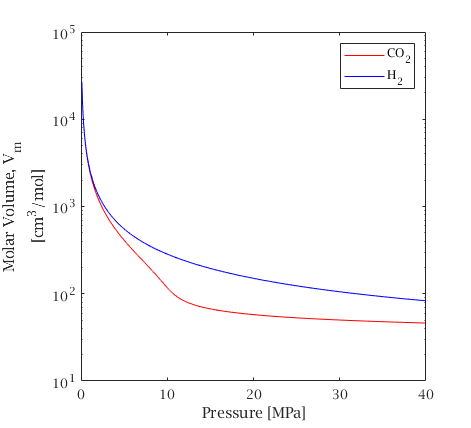
Figure 1: Molar volume values calculated via equations of state for CO₂ and H₂, under isothermal temperature of 50^oC. Molar volumes are identical at low pressures where both can be considered ideal gases.

In practice, empirical Equations of State (EoS) are used to obtain values of $V_{m}$ as a function of pressure for the bulk gas phases. Herein, we utilize the Peng-Robinson EoS [26] for CO₂; and the Abel-Noble EoS for H₂, using parameter values presented in [27]; results are shown in Figure 1. We note that although H₂ is a small molecule, as total system pressure increases, the molar volume of H₂ is significantly larger than CO₂, due to stronger attractive Van der Waals interactions between CO₂ molecules at a given pressure and temperature.

II.1 Bulk Gas and Aqueous Phases

For any static fluid or fluid component in a gravitational field $g$, conservation of energy gives the dependence of chemical potential $\mu$ on height $z$ (at constant $P$, $T$) through

$$\frac{\partial\mu}{\partial z}=m_{m}g,$$ (3)

where $m_{m}$ is the fluid component’s molar mass and $g$ is the acceleration due to gravity (herein, $g$ takes a positive value in the downwards direction and height $z$ positive upwards). Note that chemical potential is sometimes defined to exclude the of influence external fields such as gravity; for example, [20] uses this alternative definition, while in [28] it is called the physicochemical potential.

For a fluid column in equilibrium, the chemical potential is the same at all heights: $\mu(z)=\mu(z_{o})$, leading to the hydrostatic pressure gradient [29]:

$$\frac{\partial P}{\partial z}=-\rho(z)g$$ (4)

For an ideal gas (“$ig$”) this is integrated to give the barometric equation

$$\frac{P_{ig}}{P_{0}}=e^{\frac{-m_{m}g(z-z_{o})}{RT},}$$ (5)

whereas the aqueous phase can be considered an incompressible liquid with density $\rho_{w}$, independent of pressure, so the hydrostatic pressure $P_{s}$ for the aqueous solution can be calculated:

$$(P_{s}-P_{o})=-\rho_{w}g(z-z_{o}).$$ (6)

Here we define $z_{o}$ to be the height where there is mechanical equilibrium between the aqueous solution ($s$) and and bulk gas ($g$) fluid components: $P_{s}(z_{o})=P_{g}(z_{o})=P_{o}$. The difference in hydrostatic pressure gradient for the gas and aqueous solution results in mechanical disequilibrium between the fluids: $P_{g}(z)\neq P_{s}(z)$ for $z\neq z_{o}$. In unconstrained geometries, this leads to gravitational separation; however, in a porous medium, the two phases can coexist in mechanical equilibrium over a finite height range due to Young-Laplace pressure differences (eq. 1) arising from the non-wetting fluid forming bubble-like ganglia with positively-curved interfaces. This results in a height-dependent capillary pressure $P_{c}(z)=P_{g}-P_{s}$ that can compensate for the hydrostatic pressure gradient.

The bulk solute (gas phase) will generally be less dense than the aqueous phase, and is assumed to be the non-wetting fluid in a geologic porous medium. This has been established for typical conditions and geologic materials of subsurface storage projects [8]; although shifts towards intermediate-wetting have been observed [30, 31, 32], particularly when organic carbon constituents are present [33, 34]. Nonetheless, we assume water-wet conditions; and therefore a ganglion of bulk gaseous (or supercritical) fluid can only exist in contact with aqueous phase above the equilibrium height, $z\geq z_{o}$, where $P_{g}>P_{s}$ and capillary pressure can restore mechanical equilibrium. The capillary pressure must increase as the height above $z_{o}$ increases, indicating smaller and smaller radii of curvature; in pore sizes typical of storage reservoirs, mechanical equilibrium can only be maintained by capillarity for a few tens of meters. This implies that as height above $z_{o}$ increases, the water is increasingly pushed into crevices until its presence is negligible and the pore space can be considered to be filled with bulk gas phase. At depths below the equilibrium height ($z<z_{o}$) the capillary pressure would need to be negative to support coexistence - this indicates that bulk gas cannot reside $z<z_{o}$ unless supported by a reversal of wettability.

We now consider dissolved gas solute within the aqueous phase; of principal interest is the behaviour of solutions with CO₂ or H₂ dissolved in water. Since CO₂ or H₂ are only weakly soluble in water, we treat them as dilute solutions, which greatly simplifies the analysis as the solute can be treated independently of the solvent. The dependence of the chemical potential of the dissolved solute phase, $\mu_{s}$ on pressure (other variables held constant) is the equivalent of eq. 2 for a solute rather than bulk phase:

$$\frac{\partial\mu_{s}(P)}{\partial P}=\overline{V}_{m}$$ (7)

Where $\overline{V}_{m}$ is the partial molar volume of the dissolved solute; i.e. the volume occupied by a mole of gas dissolved in the aqueous phase (defined formally as the increase in volume of the solution associated with addition of a mole of solute). Note that while pure gas molar volume $V_{m}$ is clearly not constant with pressure, the partial molar volume $\overline{V}_{m}$ refers to gas dissolved in the liquid phase. While CO₂ partial molar volume has been shown to be a function of dissolved concentration and temperature [35, 36, 37], the data compilation of Garcia [37] shows that $\overline{V}_{m,CO2}$ varies only between 30-40 cm³/mol for temperatures from 0-100^oC, and the data of [36] shows only a weak dependence on aqueous composition in the concentration range of approximately 1% (molar percent); for simplicity, we don’t model variability in $\overline{V}_{m,CO2}$ in the calculations in this work. These values imply a density higher than the aqueous solvent; this negative buoyancy is the driver for downwards convection of CO₂ as well as the gravitational diffusive fluxes discussed here. To our knowledge, the variation of H₂ partial molar volume under geologically relevant pressure, temperature and concentration is not well documented.

For dilute solutions, it is assumed that the properties of the solution are not affected by the presence of the solute, and that interactions between solute molecules can be neglected. These assumptions (which also imply that $\overline{V}_{m}$ is independent of concentration, and that activity coefficients are 1) lead to the standard expression for the chemical potential of a dilute solution [29]:

$$\mu_{s}(P,x)=\mu_{s}(P,x_{o})+RT\ln\frac{x}{x_{o}},$$ (8)

where $x$ is the molar concentration, and $x_{o}$ is an arbitrary reference solute concentration.

To derive a relationship between $\mu$, $P$, $T$, $z$ and $x$, we begin with the definition of the total differential $d\mu(P,T,z,x)$:

$$d\mu(P,T,z,x)=\frac{\partial\mu}{\partial P}dP+\frac{\partial\mu}{\partial T}dT+\frac{\partial\mu}{\partial z}dz+\frac{\partial\mu}{\partial x}dx$$ (9)

We first apply this for dissolved gas, so that $\mu$ is the chemical potential of the solute $\mu_{s}$. The partial derivatives of $\mu_{s}$ with respect to pressure $P$, height $z$ and concentration $x$ are obtained, respectively, from eqns. 7, 3 and from differentiating eqn. 8; then, taking the isothermal case $dT=0$ gives the thermodynamic identity for dilute solutions in a gravitational field:

$$d\mu_{s}(P,z,x)=\overline{V}_{m}\,dP+m_{m}g\,dz+\frac{RT}{x}\,dx.$$ (10)

This can be re-written in a more convenient form, using $dP=-\rho_{w}g\,dz$ (from eq. 4 for the aqueous phase), and $m_{m}=\overline{V}_{m}\rho_{s}$ (recall that $\rho_{s}$ is the effective density of the dissolved solute):

$$d\mu_{s}(P,z,x)=\overline{V}_{m}\left(\rho_{s}-\rho_{w}\right)\,g\,dz+\frac{RT}{x}dx.$$ (11)

At equilibrium, $\mu_{s}$ does not change with height; thus, if $\rho_{s}\neq\rho_{w}$, the equilibrium concentration of dissolved solute (i.e. gas solubility) must vary with depth, in order to compensate for the effect of a gravitational field. Thus, the equilibrium concentration profile of solute $x_{e}(z)$, is obtained by imposing constant chemical potential $d\mu_{s}(z)=0$ in eq. 11:

$$\frac{1}{x_{e}}\,\frac{dx_{e}}{dz}=\frac{d(\ln x_{e})}{dz}=-\frac{\overline{V}_{m}}{RT}(\rho_{s}-\rho_{w})g$$ (12)

Approximating $\overline{V}_{m}$ to be independent of pressure (discussed below), this equation can be integrated by defining a reference height $z_{o}$ such that $x(z_{o})=x_{o}$, and integrating from $z_{o}$ to $z$ and $x_{o}$ to $x$; revealing that the gradient in concentration depends on the relative density of the dissolved phase and the water [29]:

$$x_{e}(z)=x_{e}(z_{o})e^{-\overline{V}_{m}(\rho_{s}-\rho_{w})g(z-z_{o})/RT}$$ (13)

Diffusive flux will act to establish this equilibrium distribution in the aqueous phase. Li et al. [20] provide additional description and dynamic analysis of this process (often called “sedimentation”) for CO₂ in geologic reservoirs.

The equilibrium distribution of solute concentration in the aqueous phase as a function of depth, calculated from equation 13 and using parameter values as indicated in Table 1, is shown in solid lines in Figure 2. As discussed above, we assume a constant partial molar volume for both CO₂ and H₂, while noting that this is an approximation only, with likely accuracy of around 25%. There is a single unavoidable free parameter in equation 13: the final equilibrium concentration at the reference height $x_{e}(z_{o})$, which cannot be known a-priori for a reservoir gas storage scheme. In this analysis, in order to estimate an upper bound on mass transport due to diffusion, we apply the assumption that $x_{e}(z_{o})$ is equal to the solubility limit at the pressure in the aqueous phase at a depth of 2000 m. However, this assumption is highly unlikely to be achieved in the context of CO₂ storage; instead it is more likely that there will be no depth at which the equilibrium concentration is equivalent to the fully saturated condition, as this would imply that enough CO₂ has been injected to fully saturate the formation or that downwards mass transfer due to convective dissolution has been somehow negated.

Here we highlight an important result: because dissolved CO₂ is more dense than water under typical subsurface conditions, the equilibrium CO₂ concentration increases with depth, whereas the reverse is true for H₂. Some previous work has overlooked this [19] or (assuming an ideal solution) used V_m in place of $\overline{V}_{m}$ [18] leading to erroneous conclusions that the equilibrium CO₂ concentration gradient decreases with depth (the error in [18] has been pointed out already in [20]).

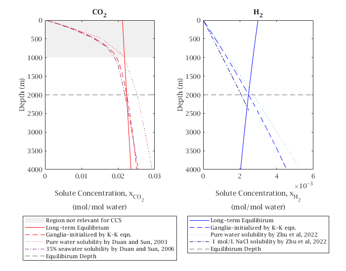
Figure 2: Initial ganglia-initialized and equilibrium aqueous concentration profiles for CO₂ and H₂ under isothermal assumption. Ganglia-initialized concentrations are calculated from the Krichevsky-Karzarnovsky equation (eq. 15). Values interpolated from literature tabulations are included for comparison for both CO₂ [38, 39] and H₂ [40] under pure water and saline conditions. Long term equilibrium shown for $\mu_{i}=\mu_{e}$ (based on the KK-concentration estimates) at $z_{1}=2000$ m (and depth = 2000 m). Note the difference in scale between CO₂ and H₂.

Equation 13 describes the final equilibrium state of the aqueous solution in a gravitational field, while equations 4, 5 and 6 give the equilibrium state of a continuous gas column (the “gas cap”). Since in both cases equilibrium derives from imposing uniform chemical potential, we can therefore also infer the equilibrium state of a multiphase fluid-porous media system consisting of both bulk and dissolved gas; if the bulk and dissolved phases are in equilibrium at any one depth, they must be in equilibrium at all depths. As depth increases, the pressure of the column of H₂ increases, and is in equilibrium with the aqueous phase which contains a decreasing concentration of H₂. For CO₂, the increasing bulk phase pressure is in equilibrium with water containing an increasing concentration of CO₂. Note that, as explained earlier, since the aqueous and gaseous phases have different densities, the phase pressures are not equal at all heights. In the presence of thermal gradients, there is no longer diffusive equilibrium between solute and continuuous gas phase, as discussed in section III.

II.2 Gas Ganglia

Now consider the non-equilibrium case where there exists a continuous aqueous liquid with dissolved solute (in a dilute solution) as the wetting phase in a porous medium, in contact with disconnected (trapped) ganglia of the solute at a height-independent capillary pressure. This scenario may arise following CO₂ or H₂ injection into an aquifer, after some re-imbibition has occurred to disconnect the gas phase. We assume that enough time has elapsed since injection for the dissolved solute to be in equilibrium with nearby trapped ganglia at the same depth, but not enough time for equilibrium between depths within the column. This residual, ganglia-initialized state is our “initial” condition, with concentration indicated as $x_{i}(z)$.

We first consider pressure dependence. Equilibrium between solute and ganglia implies that $\mu_{s}(P,x)=\mu_{g}(P)$ for all $P$, where $\mu_{g}$ is the chemical potential of the pure gas ganglia.

Therefore, integration of eq. 11 from $P_{o}$ to $P$, assuming constant $\overline{V}_{m}$ and $T$ gives:

$$\mu_{g}(P)-\mu_{g}(P_{o})=RT\ln\frac{x_{i}(P)}{x_{i}(P_{o})}+(P-P_{o})\overline{V}_{m}$$ (14)

Using the fact that chemical potential $\mu_{g}$ and fugacity $f_{g}$ of the bulk phase in the ganglia are related through $\mu_{g}=RT\ln f_{g}+\text{const.}$, we see that this is the Krichevsky-Karzarnovsky equation [25], a high-pressure generalisation of Henry’s law:

$$RT\ln\frac{f_{g}(P)}{x(P)}=RT\ln K+(P-P_{\text{vap}_{w}})\overline{V}_{m},$$ (15)

where $K$ is the Henry’s law coefficient, generalised for real gases:

$$K=\lim_{x\rightarrow 0}\frac{f_{g}}{x}$$

and $P_{\text{vap}_{w}}$ is the vapour pressure of the solvent (water); it is insignificant for our system – and neglected elsewhere in this work – but necessary in general because in the limit of zero solute concentration $x\rightarrow 0$ the ganglia are composed entirely of water vapour, so $(P-P_{\text{vap}_{w}})\rightarrow 0$. We note that the Krichevsky-Karzarnovsky equation was originally derived to describe the H₂-water (and N₂-water) system [25]; additionally, previous analysis of experimental data has concluded that the CO₂-water system is accurately modelled by the Krichevsky-Karzarnovsky equation for temperatures less than 100^o C; at higher temperatures the activity of dissolved CO₂ must also be taken into account [41].

With fugacity calculated from the EoSs noted above, we use eqn. 15 to determine the partitioning relationship between concentration and fugacity of the pure gas phase over our considered range of depths (3). Fugacity coefficient is defined as the ratio of fugacity to system pressure, $\phi=\frac{f}{P}$. Partition coefficients (ratios quantifying how a species will be distributed in two phases at equilibrium) calculated from eq. 15 are presented as gas phase fugacity to aqueous solubility, with units of $\frac{MPa}{\text{mol gas / mol aq. phase}}$, simplified to MPa.

Note that fugacity – in this case, the equivalent pressure exhibited by the gas for phase partitioning purposes – shows opposing behaviour for H₂ and CO₂. For H₂, the bulk gas phase behaves as though it is at higher pressure than the system pressure; the opposite is the case for CO₂. H₂ shows a much stronger affinity to partition into the bulk gas phase (i.e. it has a much lower dissolved concentration at the same pressure); and a more extreme variation in partitioning with depth.

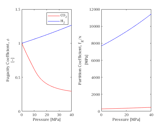
Figure 3: Calculation of gas fugacity coefficients from EoSs, and gas-solution partition coefficients from the Krichevsky-Karzarnovsky equation (eq. 15) under isothermal temperature conditions of 50^oC.

By applying eq. 9 for the chemical potential of the bulk gas phase $\mu_{g}$, we can use eqs. 2 and 3 to obtain a thermodynamic identity for a column of bulk gas phase (assuming pure phase - i.e. neglecting the small fraction of water vapour)

$$d\mu_{g}(P,z)=V_{m}dP+m_{m}gdz.$$ (16)

Relating 11 and 16 by imposing equilibrium between the ganglia and the dissolved solute at all depths, $\mu_{s}(z,x)=\mu_{g}(z)$, and simplifying gives the vertical concentration gradient

$$RT\frac{1}{x_{i}}\frac{dx_{i}}{dz}=RT\frac{d(\ln x_{i})}{dz}=-\left(V_{m}-\overline{V}_{m}\right)\rho_{w}g,$$ (17)

which is determined by the density difference between the bulk and dissolved phases. In all typical scenarios, the dissolved phase will be more dense than the bulk gas phase ($V_{m}-\overline{V}_{m}>0$), so this initial concentration gradient will increase downwards.

To illustrate the ganglia-initialized aqueous solute concentration distribution, we first estimate that ganglia pressure is 100 kPa higher than the hydrostatic pressure (to account for Laplace pressure of the gas ganglia); this is significantly higher than would generally be expected based on capillary pressure-saturation relationships for model quarry sandstones (e.g. [42, 14]) but this overestimate has no impact on our findings. Then, converting the ganglia pressure to fugacity, $f$, through the EoSs and applying the Krichevsky-Karzarnovsky derived partition coefficient, we arrive at an aqueous concentration value that would be present in the local aqueous phase equilibrated with these ganglia (Figure 2). Note that the same result is obtained by numerical integration of eq. 17 using values for $V_{m}$ from the EoS. In Figure 2 we also plot concentration values derived from interpolation of literature tabulations; including CO₂ solubility in pure water [38], CO₂ solubility in seawater-type brine [39], and H₂ solubility in pure water and 1 mol/kg NaCl [40]. In the isothermal case, the concentrations estimated via eq. 15 are quite similar to the literature results, despite the fact that the Krichevsky-Karzarnovsky equation includes no correction for activity.

Comparison of the ganglia-initialized and equilibrium concentrations shows the direction of the concentration difference driving diffusive transport. Diffusion will drive the system from the concentration gradient described by eq. 17 (the ganglia-initialized state) to the global equilibrium gradient of eq. 13 (the final state). Setting a reference height $z_{1}$ to be the point where the initial and final concentrations are the same (labeled “Equilibirum Depth” in Figure 2); then, above $z_{1}$ the initial concentration is lower than the final state - there must be an influx of dissolved gas. Below $z_{1}$ the initial concentration is higher than the final state - gas must be depleted to reach equilibrium. This implies upward migration of solute in all isothermal cases, even though the equilibrium concentration is increasing downwards for CO₂.

This conceptual description of the system in terms of concentrations is intuitive, and it is accurate in the isothermal case regardless of selection of equilibrium height $z_{1}$ because concentration profiles are monotonic with depth. However, we caution that this logic can only be applied when both initial and equilibrium concentration profiles are monotonic. We will show in section III that for non-monotonic concentration gradients, the direction of diffusion cannot easily be inferred, because the concentration difference between initial and equilibrium states depends on the choice of $z_{1}$. Instead, it is more useful to directly interrogate the chemical potential of the system. From eq. 11:

$$\frac{d\mu_{si}}{dz}=(\rho_{s}-\rho_{w})g\,\overline{V}_{m}+RT\frac{d}{dz}ln(x_{i})$$ (18)

This can be simplified by writing the concentration gradient term using eq. 17 and using the fact that $\rho_{s}\overline{V}_{m}=m_{m}=\rho_{g}V_{m}$:

$$\frac{d\mu_{s}}{dz}=(\rho_{g}-\rho_{w})g\,V_{m}$$ (19)

This reveals that the chemical potential gradient is controlled by the difference in density between the bulk gas and the aqueous solution, and since $\rho_{g}<\rho_{w}$ for CO₂ and H₂, the chemical potential of dissolved solute in the ganglia-initialized state decreases with $z$ (i.e. increases with depth). Under global equilibrium, $\mu_{s}$ is the same everywhere and $d\mu_{s}/dz=0$ – comparison of these two gradients demonstrates that diffusion must act upwards, as described earlier. In general, in the isothermal case: for any fluid that is less dense than the aqueous phase, the concentration in local equilibrium with trapped ganglia increases with depth more quickly than the global equilibrium concentration. Therefore Ostwald ripening will occur upwards for isothermal dilute solutions of all fluids less dense than brine.

In summary, under the assumptions of dilute solution, constant partial molar volume, and isothermal conditions; we find that:

1. In global equilibrium, $\mu_{s}(z)=\text{const.}$, and the dissolved concentration gradient is proportional to $-(\rho_{s}-\rho_{w})$; thus x${}_{H_{2}}$ and x${}_{CO_{2}}$ have opposing gradients.

2. For a solution in local equilibrium with trapped ganglia $\mu_{si}(z)=\mu_{g}(z)$; chemical potential gradient is proportional to $(\rho_{s}-\rho_{g})$; i.e. $\mu_{si}$ increases downwards for both H₂ and CO₂, driving upwards diffusive mass transport of both H₂ and CO₂ under isothermal conditions.

This analysis thus echos previous studies finding upwards transport due to Ostwald ripening in isothermal systems [18, 16, 17, 19, 20].

Table 1: Parameters used in numerical estimates

Parameter
Aqueous Density [kg/cm3]a	1.050 $\times$ 10${}^{-}3$
Aqueous Molar Volume [cm3/mol]	18.07
Acceleration of Gravity [m/s2]	9.81
Isothermal Temperature [oC]a	50
Non-isothermal Surface Temperature [oC]	25
Vapor Pressure of Water [MPa]	0.012b
Parameter	CO2	H2
Henry’s Law Constant, 50oC c [MPa]	281	7683
Partial Molar Volume [cm3/mol]	35.1d	26.7e
Molar Mass [kg/mol]	0.044	0.002
Diffusion Coefficient (pure water, 25oC) [m2/s]	$2.2\times 10^{-9}$f	$5.11\times 10^{-9}$g
Critical Temperature [oC]	30.978	-239.95
Critical Pressure [MPa]	7.38	1.30
Acentric Factorh [-]	0.228	-0.220

• a. Assumed, following [19].

• b. [43]

• c. Calculated from values presented in [44] and converted to pressure units using presented values for brine.

• d. [37]

• e. [45]

• f. [46]
  

• g. [47]

• h. [48]

III Impact of Temperature Gradients

Geologic storage will, of course, be affected by geothermal gradients. The non-isothermal case adds significant challenges to the analysis and relatively few works have analysed the impact of typical geothermal gradients. Li et al. [20] provide an initial treatment of non-isothermal conditions; while they pointed out that this treatment requires taking into account thermodiffusion (the Soret effect), they did not include it in their models due to the scarcity of data on thermodiffusion in CO₂-water system; instead their model only accounted for thermal gradients by incorporating the change in solubility with depth. Their results showed thermal gradients suppress diffusive fluxes; and under certain rare conditions, have the potential to reverse their direction - i.e. for CO₂ to flow downwards. As we show later, the simplified analysis in Li et al. [20] greatly underestimates the effect of geothermal gradients; in fact, fluxes reverse direction for low to moderate geothermal gradients (diffusive transport is downwards for both gases) and rates may increase by an order of magnitude when the entropic impacts on chemical potential are properly considered.

Following the work of Li et al. [20], Coelho et al. [23, 24] conducted non-equilibrium molecular dynamics (NEMD) simulations to determine the Soret coefficient of CO₂ in water and brine at reservoir conditions. Their values for pure water corroborate experimental results from Guo et al. [49]; while there is still significant uncertainty, the effects of thermodiffusion on CO₂ storage can now be estimated quantitatively. Coelho et al. [23, 24] also conducted a partial analysis of CO₂ diffusive fluxes, incorrectly assuming that CO₂ thermophobicity would necessarily drive CO₂ upwards under geothermal gradients. To our knowledge, Soret coefficients for H₂ under reservoir-relevant temperatures and pressures are still not well characterized.

There has been significant debate about whether thermodiffusion must be treated as a non-equilibrium kinetic phenomenon, or can be treated by local thermodynamic equilibrium [50, 51]. Kocherginsky and Gruebele [28, 52, 53] have made significant progress on developing local equilibrium theory of thermodiffusion and conclude that it is valid given the following assumptions [53]:

1. transport is diffusive without hydrodynamic contributions;

2. particle numbers $N_{i}$ in a volume $\delta V(z)$ under consideration are large enough ($N_{i}\gg\sqrt{N_{i}}$).

3. local average thermodynamic variables remain meaningful; and the shortest time scale $\delta t$ is long enough so that the local equilibrium may be assumed: a local temperature $T(x)$ and concentration $c(z)$ can be defined in each volume $\delta V$.

Condition 1 is a fundamental assumption of this work due to its focus on diffusive transport: we assume that there is no advective or convective transport within the storage reservoir. The remaining two conditions will clearly be valid for subsurface storage environments where thermal gradients are some decades of degrees per kilometer.

Therefore, we treat the non-isothermal case by assuming the reservoir consists of vertical subsections in local thermodynamic equilibrium. Return to eq. 9 where, rather than assuming $dT=0$, we assume a thermal gradient $T^{\prime}(z)$ such that $dT=T^{\prime}dz$.

First, considering the dissolved gas phase and using the definition of partial molar entropy $\overline{S}_{m}$ from the thermodynamic identity:

$$\frac{\partial\mu_{s}}{\partial T}=-\overline{S}_{m},$$

gives the generalization of equation 11 for non-constant $T$:

$$d\mu_{s}=-\overline{V}_{m}(\rho_{s}-\rho_{w})g\,dz-\overline{S}_{m}T^{\prime}dz+\frac{RT}{x}\,dx.$$ (20)

Within the above-stated assumptions we can associate the partial molar entropy with the Soret coefficient $\mathcal{\mathcal{S_{T}}}$ [53]:

$$\mathcal{\mathcal{S_{T}}}=-\frac{\overline{S}_{m}}{RT}$$ (21)

As mentioned above, the value of $\mathcal{S_{T}}$ for supercritical CO₂-water systems has only recently been determined, through the experimental work of Guo et al. [49] and computational works of Coelho et al. [23, 24]. These works agree on the magnitude and trend of the Soret coefficient, finding that $\mathcal{S_{T}}$ for CO₂ in pure water is positive with values between $0.01-0.03$ K^-1 at lower temperatures, and transitions to negative values in the region 370-400 K; note: a positive Soret coefficient implies a tendency to migrate to lower temperature regions. The impact of salts has been estimated by Coelho et al. [24], who show a less positive $\mathcal{S_{T}}$, transitioning to negative values at lower $T$. Earlier, Windisch et al. [54] had not found a Soret coefficient significantly different than zero, but this work had a very large uncertainty so is consistent with the values of refs Guo et al. [49] and Coelho et al. [23, 24].

The concentration gradient in the final equilibrium state for non-constant $T$, obtained by setting $d\mu_{s}=0$ (global diffusive equilibrium) in eq. 20, is:

$$\frac{d(\ln x_{e})}{dz}=-\frac{\overline{V}_{m}}{RT}(\rho_{s}-\rho_{w})g-\mathcal{S_{T}}T^{\prime}.$$ (22)

As discussed, for CO₂ where $\rho_{s}>\rho_{w}$, the first term is negative, leading to negative concentration gradient (increasing with depth) for the isothermal case $T^{\prime}=0$.

However, the additional term is positive at lower temperatures (where $\mathcal{S_{T}}>0$), since $T$ increasing with depth implies $T^{\prime}<0$. In Figure 4 we display the relative size of the gravitational and thermal contributions to eq. 22 for a range of depths, using the Soret relationship for CO₂ in 1 mol/kg NaCl brine from Coelho et al. [24], for isothermal conditions as well as typical geothermal gradients of 10 ^oC/km and 30 ^oC/km. The Soret effect does not exist in isothermal conditions, hence the 0 thermal term in the leftmost column. The gravitational term exists as a negative term under all temperature conditions; however, its magnitude remains on the order of $10^{-5}$ m^-1 – too small to be seen - and its contribution is completely overwhelmed by the Soret effect in non-isothermal cases. We note that similar estimates are not available for H₂ due to the absence of published Soret coefficient data for aqueous solutions of H₂.

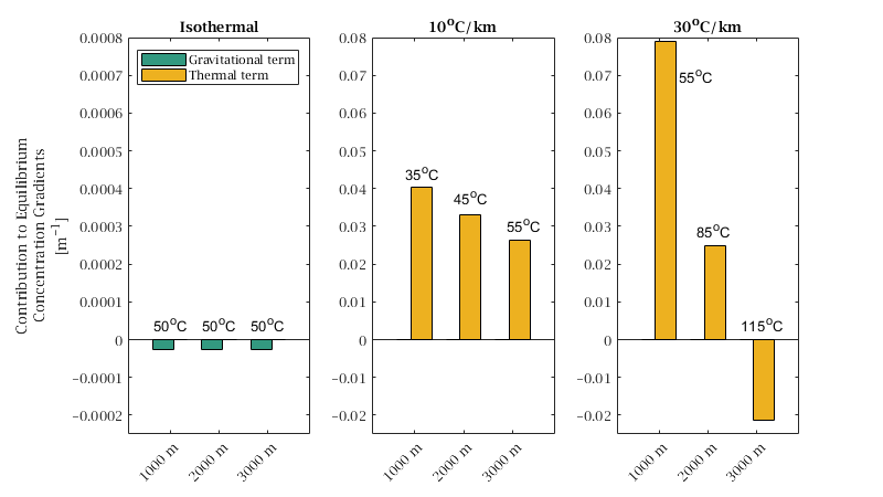
Figure 4: Contributions of gravitational and thermal terms to the gradient of natural logarithm of concentration at equilibrium (eq. 22). Note that the y-axis for the isothermal condition is an order of magnitude smaller than the cases with a geothermal gradient. The gravitational contribution is present in all cases, but too small to be visible under scenarios with a geothermal gradient.

The thermodiffusion term will be sufficient to invert the concentration gradient in regions of the reservoir: equilibrium CO₂ concentrations will decrease with depth in middle-upper regions of reservoirs that have a typical geothermal gradient, before increasing again once the Soret coefficient transitions to negative values. While these qualitative statements can be made, quantitative estimates of the equilibrium concentration profile have very high uncertainty, since numerical integration of eq. 22 amplifies the uncertainties in $\mathcal{S_{T}}$. As we show below, the equilibrium concentration profile is, in fact, not significant in determining the direction of diffusive flux for either CO₂ or H₂, because it is not the gradient of concentration that determines the direction of diffusive flux, but the gradient of chemical potential.

For the gas phase, equation 16 is modified by a similar additional term for the non-isothermal case:

$$d\mu_{g}(P,z)=V_{m}dP-S_{m}T^{\prime}dz-m_{m}gdz.$$ (23)

Where $S_{m}$ is the molar entropy of the gas phase.

As for the isothermal case, the ganglia-initialized (residual-state) concentration gradient in equilibrium with the gas ganglia is obtained by equating the gas and solute chemical potential from eqs. 20 and 23:

$$RT\frac{d(\ln x_{i})}{dz}=-\left(V_{m}-\overline{V}_{m}\right)\rho_{w}g-(S_{m}-\overline{S}_{m})T^{\prime}$$ (24)

Differentiating eq. 20 and using eq. 23 gives the chemical potential gradient for gas molecules in the ganglia-initialized solution:

$$\frac{d\mu_{s_{i}}}{dz}=(\rho_{g}-\rho_{w})gV_{m}-S_{m}T^{\prime}$$ (25)

This will be proportional to the diffusive flux of a ganglia-initialised system, which will be discussed further in section IV.

Equation 25 relies only on the assumptions of dilute solution and local thermodynamic equilibrium. It is noteworthy that the diffusive flux of dissolved gas from a ganglia-initialised residual state is independent of the Soret coefficient of the dissolved gas. Since the temperature profile is the same for the ganglia-initialised and equilibrium states, the Soret effect, which depends only on temperature, cancels out as it makes an equal contribution to the concentration profiles in both cases. With the Soret effect not playing a role, the flux is determined by how chemical potential varies with depth in the bulk gas ganglia. Sufficient contribution by the entropic term $-S_{m}T^{\prime}$ causes a positive gradient in $\mu_{g}$=$\mu_{si}$, due to the positive entropy of the bulk gas and negative $T^{\prime}$. For large enough $-S_{m}T^{\prime}$, this leads to free energy decreasing with increasing depth because the temperature dependence of the $-TS$ term outweighs the pressure dependence in the $PV$ term.

In order to calculate the impact of thermal gradients, We obtain values for molar entropy $S_{m}$ for CO₂ and H₂ under our considered pressure and temperature conditions via the following steps. The molar entropy for an ideal gas ($S^{ig}$) at a given temperature ($S^{ig}_{T}$)is found using the Shomate equation with parameters tabulated by [44], calculated from data originally from Chase [55], and modified for pressure through $S^{ig}=S^{ig}_{T}-Rln(P/P_{R})$ ($P_{R}$ is the reduced pressure $P/P_{c}$ where $P_{c}$ is the pressure at the critical point). Deviation from the ideal gas value is found using a departure function [56, 57], calculated using the compressibility factor and constants calculated in the Peng-Robinson EOS [26]. Under our considered conditions, CO₂ molar entropy ranges from approximately 140-220 J/mol-K, and H₂ from 80-110 J/mol-K; these calculated values are consistent with tabulated data [58] to approx. 2%. Higher pressure decreases the molar entropy while higher temperature increases molar entropy; the relationship of entropy to depth is thus nontrivial and dependent on geothermal gradient (Figure 5).

The real-gas calculated entropy values are sufficient to reverse the chemical potential gradient for CO₂ at relatively shallow depths, even for low geothermal gradients; for H₂, a gradient of 10^oC is insufficient to reverse the gradient, but 30^oC suffices (Figure 6). Recall that positive $d\mu_{s_{i}}/dz$ indicates chemical potential increasing upwards, and therefore induces downwards-driven diffusion. Larger geothermal gradients generate higher positive gradients and shift the crossover point to shallower depths. At shallow depths <1000 m, the molar volume of the gas phase varies significantly, leading to large negative gradients. Upwards diffusive transport is thus favored in very shallow regions; however, these depths are generally not relevant for gas storage schemes.

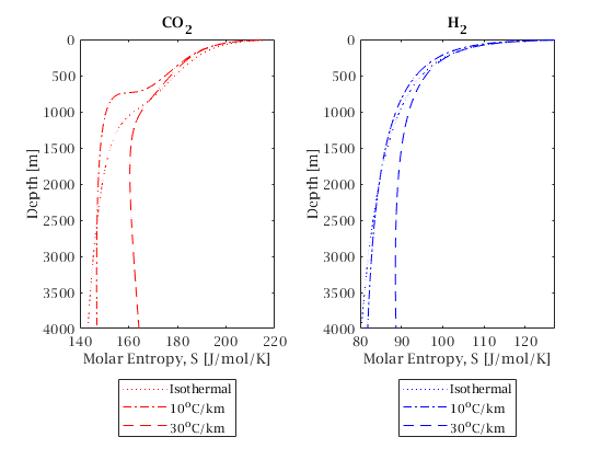
Figure 5: Variation of CO₂ and H₂ bulk molar entropy with depth for various geothermal gradients.

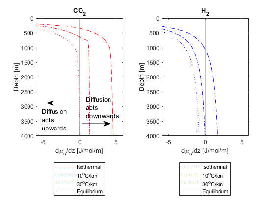
Figure 6: Variation of the vertical gradient of chemical potential with depth for the ganglia-initialized state under different thermal assumptions, indicating the direction of diffusive flux. A positive value indicates that chemical potential is increasing with $z$ (i.e. decreasing with depth) – resulting in downward net diffusion of dissolved gas molecules.

In Figure 7, we present curves of the ganglia-initialized chemical potential ($\mu_{si}$) vs. depth, calculated through numerical integration of eq. 25. With these figures, we return to the conceptual model presented in Section II. At equilibirum, the chemical potential $\mu_{se}$ will be equal at all depths, i.e. present as a vertical line in Figure 7. The precise value at equilibrium does not need to be determined a-prioi, it is sufficient to know that it will be between the minimum and maximum values of $\mu_{si}$. For regions where $\mu_{si}>\mu_{se}$, the chemical potential must decrease to reach equilibrium and molecules will diffuse away; where $\mu_{si}<\mu_{se}$, there must be an influx to reach equilibrium. For curves where $\mu_{si}$ monotonically increases with depth (CO₂ and H₂ under isothermal conditions, and H₂ at $-T^{\prime}=10^{o}$C), there must be diffusive transport upwards. However, for non-monotonic curves, it is possible for transport to be both upwards (for shallow depths above the inflection point) and downwards (for all depths below the inflection point). For carbon storage, reservoirs at depths below 1000 m are targeted; thus, only downwards diffusion is expected for any realistic carbon storage situation.

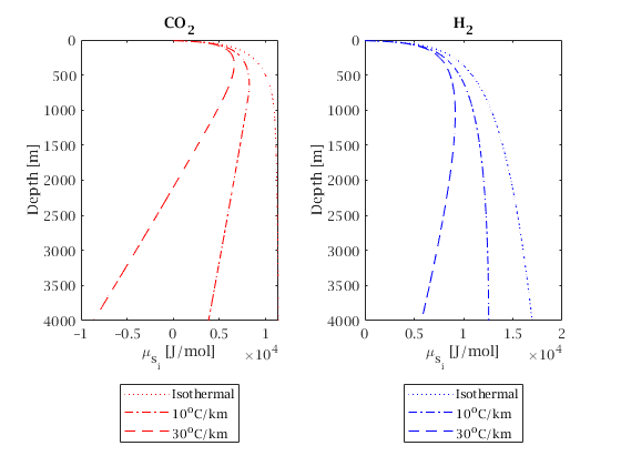
Figure 7: Variation of chemical potential $\mu_{si}$ of the ganglia-initialized system with depth. The equilibrium condition would be represented by constant $\mu$ (vertical line). The direction of diffusive flux is thus given by the sign of the gradient $d\mu_{s}/dz=0$: for $\mu_{s}$ increasing with $z$ (decreasing with depth), diffusion acts downwards, according to eq. 27.

It is also worth mentioning the behaviour in the upper part of the reservoir where there is continuous gas. In the presence of geothermal gradients, it is not possible for a column of gas in mechanical equilibrium ($dP=-\rho_{g}gdz$) to also be in diffusive equilibrium; eq. 23 gives for the “equilibrium” chemical potential $\mu_{g_{e}}$:

$$\frac{d\mu_{g_{e}}}{dz}=-S_{m}T^{\prime}$$ (26)

Again we see a positive gradient with $z$. This will tend to cause ex-solution at the bottom of the ganglion (lower chemical potential in the gas phase) and dissolution at the top, creating a cyclic transport of gas molecules: hydrodynamic upward flow within the gas phase and downward diffusive transport of dissolved molecules within the aqueous phase. This is effectively the same as the process described in Blunt [19] for the isothermal case (erroneously, as there is equilibrium in that case). Energy for the continual motion of gas molecules comes from the continual heat flux through the reservoir.

IV Kinetics of Diffusion

Flux in this diffusion-controlled system will be described by:

$$J(z)=\frac{-\mathcal{D}_{x}(z)}{RT(z)}\frac{d\mu_{si}}{dz}$$ (27)

This expression is different from the empirically-derived Fick’s first law (i.e. $J=-\mathcal{D}\frac{dx}{dz}$) because in this system, the gradient of chemical potential $\mu_{s}$ driving diffusion is not only a function of concentration $x(z)$, but also has a significant contribution due to the gravitational field and temperature gradient.

Here we assume that the diffusion coefficient, $\mathcal{D}$ is independent of concentration and pressure, but does increase with temperature following the Stokes-Einstein equation:

$$\mathcal{D}_{T(x)}=\mathcal{D}_{T=25^{o}C}\frac{T(x)}{298K}\frac{\mu_{T=25^{o}C}}{\mu_{T(x)}}$$ (28)

Where $\mu_{T}$ is the dynamic viscosity of water; viscosity ratios were calculated via the correlation presented in Kestin et al. [59]. Diffusion coefficients were thus calculated based on the values presented in Table 1; for the 10^oC/km and 30^oC/km geothermal cases, diffusion coefficients increase by a factor of approx. 2.3 and 6.3 respectively over the depth range investigated. Following the analysis of Blunt [19], diffusion coefficients are multiplied by an assumed porosity value of 0.2 to adjust for diffusion within porous media; this also should be an upper bound as it neglects any reduction in diffusion due to tortuosity.

The maximum diffusive flux will occur when the chemical potential gradient $d\mu/dz$ is largest, i.e. at the ganglia-initialized state. In Figure 8, we provide estimates for flux of CO₂ and H₂ based on equations 27 and 19. Here, to provide an upper bound on flux estimates, we assign $x(z)$ to be the gas solubility in pure water at the depth-defined temperature and pressure, with $x_{CO_{2}}(z)$ interpolated from data reported by Duan and Sun [38] and $x_{H_{2}}(z)$ interpolated from Zhu et al. [40]. The units of $x(z)$ in eq. 27 are mol/volume, in contrast to the rest of the manuscript.

As shown in Figure 8, diffusive flux in the isothermal case is always positive (diffusion transports molecules upwards), and estimated values for CO₂ and H₂ are similar (in the region relevant to storage of both gases), on the order of $10^{-15}-10^{-14}$ mol/cm²/s. As observed above, flux quickly becomes negative (diffusive transport is downwards) for CO₂ under even the low geothermal gradient of 10^oC/km; H₂ shows a more subtle dependence, only achieving negative fluxes below 1000 m for the 30^oC/km case. In the geothermal gradient case (30^oC), downwards CO₂ flux is several times larger than the flux of H₂; its magnitude is an order larger than the isothermal CO₂ case, on the order of $10^{-13}$ mol/cm²/s.

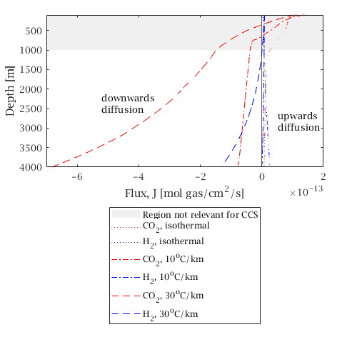
Figure 8: Diffusive flux as a function of depth for the ganglia-initialized state. Positive flux indicates upwards transport, negative flux indicates downwards.

IV.1 Comparison with Mass Transport via Convective Dissolution

Neufeld et al. [9] estimated a convective CO₂ flux equalling 20 kg m^-2 yr^-1 for the Sleipner site in the North sea, which is equivalent to 1.44$\times$10^-9 mol CO₂/cm²/s. Compared to the upper limit of the diffusive CO₂ flux estimated above, the convective flux is $\approx 4$ orders of magnitude larger (depending on temperature assumption), indicating that even for the maximal assumptions considered above, diffusive transport of CO₂ will be a minor factor. Li et al. provide a more thorough analysis of convective transport rates for a range of scenarios and similarly conclude that convective transport is likely to initiate and complete well before diffusive transport becomes significant, for almost all scenarios considered [20]. However, it is important to note that in situations with positive geothermal gradients (i.e. all likely storage reservoirs) , we predict that diffusion will drive CO₂ downwards, thus increasing storage security – in the geothermal case, diffusion and convection of CO₂ are not acting in competing directions.

As noted in Section II above, the partial molar volume of H₂ dissolved in water is larger than pure water, while the opposite is true for CO₂; i.e. water containing dissolved CO₂ is more dense and water containing dissolved H₂ is less dense than pure water. This indicates that while convective dissolution will drive mass transport of CO₂ downwards, the same process should drive H₂ upwards. Estimates of upward H₂ flux due to this process are outside the scope of this study; however, our analysis shows that in more shallow and lower-temperature reservoirs, diffusive transport will drive hydrogen upwards, again demonstrating that convection and diffusion act in the same direction. Our analysis indicates that it would require significantly deeper and warmer reservoirs to invert the H₂ diffusive flux directionality. Additional study is needed to determine the comparative importance of convective and diffusive processes for application to underground hydrogen storage.

V Conclusions

We have presented an analysis of diffusive transport in geologic storage scenarios. We detail the thermodynamic derivation of the phenomenon, taking into account the non-ideality of supercritical fluids (i.e. H₂ and CO₂) stored under high pressure in geologic formations. We show that under the assumption of isothermal conditions, diffusion drives injected gas molecules upwards, echoing previous analysis of the process of “Ostwald ripening” [18, 16, 17, 19, 20].

However, our main contribution is in the incorporation of temperature variation via geothermal gradients. We demonstrate that with more complete consideration of entropic constributions to free energies, diffusive transport reverses direction under low to moderate geothermal gradients at storage-relevant depths; furthermore, the magnitude of flux can increase by up to two orders of magnitude. Because the entropic contribution relative to the gravitational contribution is larger for CO₂ than H₂, this reversal happens at lower temperature gradients and shallower depths for CO₂, with practical impacts to storage operations. Our analysis indicates that in CO₂ storage scenarios, diffusive transport will invariably be downwards, along with convective transport; thus both mechanisms increase the storage security of CO₂ storage. In H₂ storage systems, which are likely to be more shallow and less warm, diffusive transport will likely move gas upwards (again, in concert with convective dissolution); thereby making H₂ recovery more favorable.

We provide an upper estimate for flux rates, using assumptions favorable to faster diffusion. The maximum diffusive flux estimated for CO₂ occurs under our largest investigated geothermal gradient of 30^oC and is on the order of 10^-13 mol/cm²/s; four orders of magnitude smaller than the downwards convective flux estimated for CO₂ by Neufeld et al. [9]. In this case, both diffusion and convection act in concert to drive CO₂ downwards.

Our analysis has relaxed many of the assumptions prior studies have made; particularly with respect to the isothermal temperature assumption and the ideality of the gas (supercritical) phases. However, the analysis does employ two key assumptions: (1) dilute solutions, implying unity activity coefficients, and (2) local thermodynamic equilibrium in non-isothermal cases. We have also used a single representative value for partial molar volume in all our calculations. At depths greater than those considered here, it is possible for CO₂ partial molar volume to increase to a point that the effective density of the solution is no longer greater than pure aqueous phase density, at which point the gravitational driver may reverse. Our results show that this is unlikely to impact diffusive transport of since the entropic contributions overwhelm the gravitational contributions in all storage-relevant conditions for CO₂. However, this density inversion at extreme depths will have a major overall impact as it will cause a reversal of convective fluxes, likely creating a barrier to convection.

Under these assumptions, we find that (contrary to previous studies) diffusion and convection will tend to work in concert - both driving CO₂ downwards, and both driving H₂ upwards - for conditions representative of their respective storage reservoirs (i.e CO₂ in deeper reservoirs, and H₂ in more shallow formations). While still slow, diffusive transport is thus predicted to be beneficial for both carbon storage and hydrogen storage technologies.

References

- Bachu [2008] S. Bachu, CO2 storage in geological media: Role, means, status and barriers to deployment, Progress in Energy and Combustion Science 34, 254 (2008).
- Bui et al. [2018] M. Bui, C. S. Adjiman, A. Bardow, E. J. Anthony, A. Boston, S. Brown, P. S. Fennell, S. Fuss, A. Galindo, L. A. Hackett, J. P. Hallett, H. J. Herzog, G. Jackson, J. Kemper, S. C. Krevor, G. C. Maitland, M. Matuszewski, I. S. Metcalfe, C. Petit, G. Puxty, J. Reimer, D. M. Reiner, E. S. Rubin, S. A. Scott, N. Shah, B. Smit, J. P. Trusler, P. Webley, J. Wilcox, and N. Mac Dowell, Carbon capture and storage (CCS): The way forward (2018).
- Epelle et al. [2022] E. I. Epelle, W. Obande, G. A. Udourioh, I. C. Afolabi, K. S. Desongu, U. Orivri, B. Gunes, and J. A. Okolie, Perspectives and prospects of underground hydrogen storage and natural hydrogen (2022).
- Tarkowski and Uliasz-Misiak [2022] R. Tarkowski and B. Uliasz-Misiak, Towards underground hydrogen storage: A review of barriers, Renewable and Sustainable Energy Reviews 162, 112451 (2022).
- Krevor et al. [2023] S. Krevor, H. de Coninck, S. E. Gasda, N. S. Ghaleigh, V. de Gooyert, H. Hajibeygi, R. Juanes, J. Neufeld, J. J. Roberts, and F. Swennenhuis, Subsurface carbon dioxide and hydrogen storage for a sustainable energy future, Nature Reviews Earth & Environment 2023 4:2 4, 102 (2023).
- Yang et al. [2023] B. Yang, C. Shao, X. Hu, M. R. Ngata, and M. D. Aminu, Advances in Carbon Dioxide Storage Projects: Assessment and Perspectives, Energy and Fuels 37, 1757 (2023).
- US DOE NETL [2015] US DOE NETL, U.S. Department of Energy-National Energy Technology Laboratory-Office of Fossil Energy, Tech. Rep. (U.S. Department of Energy-National Energy Technology Laboratory-Office of Fossil Energy, 2015).
- Krevor et al. [2015] S. C. Krevor, M. J. Blunt, S. M. Benson, C. H. Pentland, C. Reynolds, A. Al-Menhali, and B. Niu, Capillary trapping for geologic carbon dioxide storage - From pore scale physics to field scale implications, International Journal of Greenhouse Gas Control 40, 221 (2015).
- Neufeld et al. [2010] J. A. Neufeld, M. A. Hesse, A. Riaz, M. A. Hallworth, H. A. Tchelepi, and H. E. Huppert, Convective dissolution of carbon dioxide in saline aquifers, Geophysical Research Letters 37 (2010).
- Emami-Meybodi et al. [2015] H. Emami-Meybodi, H. Hassanzadeh, C. P. Green, and J. Ennis-King, Convective dissolution of CO2 in saline aquifers: Progress in modeling and experiments, International Journal of Greenhouse Gas Control 40, 238 (2015).
- Rezk et al. [2022] M. G. Rezk, J. Foroozesh, A. Abdulrahman, and J. Gholinezhad, CO2Diffusion and Dispersion in Porous Media: Review of Advances in Experimental Measurements and Mathematical Models, Energy and Fuels 36, 133 (2022).
- Armstrong et al. [2014] R. T. Armstrong, A. Georgiadis, H. Ott, D. Klemin, and S. Berg, Critical capillary number: Desaturation studied with fast X-ray computed microtomography, Geophysical Research Letters 41, 55 (2014).
- Andrew et al. [2014] M. Andrew, B. Bijeljic, and M. J. Blunt, Pore-by-pore capillary pressure measurements using X-ray microtomography at reservoir conditions: Curvature, snap-off, and remobilization of residual CO 2, Water Resources Research 50, 8760 (2014).
- Herring et al. [2017] A. L. Herring, J. Middleton, R. Walsh, A. Kingston, and A. Sheppard, Flow Rate Impacts on Capillary Pressure and Interface Curvature of Connected and Disconnected Fluid Phases during Multiphase Flow in Sandstone, Advances in Water Resources 10.1016/j.advwatres.2017.05.011 (2017).
- Garing et al. [2017] C. Garing, J. A. de Chalendar, M. Voltolini, J. B. Ajo-Franklin, and S. M. Benson, Pore-scale capillary pressure analysis using multi-scale X-ray micromotography, Advances in Water Resources 104, 223 (2017).
- De Chalendar et al. [2017] J. A. De Chalendar, C. Garing, and S. M. Benson, Pore-scale Considerations on Ostwald Ripening in Rocks, in Energy Procedia, Vol. 114 (Elsevier Ltd, 2017) pp. 4857–4864.
- De Chalendar et al. [2018] J. A. De Chalendar, C. Garing, and S. M. Benson, Pore-scale modelling of Ostwald ripening, Journal of Fluid Mechanics 835, 363 (2018).
- Xu et al. [2019] K. Xu, Y. Mehmani, L. Shang, and Q. Xiong, Gravity‐Induced Bubble Ripening in Porous Media and Its Impact on Capillary Trapping Stability, Geophysical Research Letters 46, 13804 (2019).
- Blunt [2022] M. J. Blunt, Ostwald ripening and gravitational equilibrium: Implications for long-term subsurface gas storage, Physical Review E 106, 10.1103/PhysRevE.106.045103 (2022).
- Li et al. [2022] Y. Li, F. M. Orr, and S. M. Benson, Long-Term Redistribution of Residual Gas Due to Non-convective Transport in the Aqueous Phase, Transport in Porous Media 141, 231 (2022).
- Zhang et al. [2023] Y. Zhang, B. Bijeljic, Y. Gao, S. Goodarzi, S. Foroughi, and M. J. Blunt, Pore-Scale Observations of Hydrogen Trapping and Migration in Porous Rock: Demonstrating the Effect of Ostwald Ripening, Geophysical Research Letters 50, 10.1029/2022GL102383 (2023).
- Goodarzi et al. [2024] S. Goodarzi, Y. Zhang, S. Foroughi, B. Bijeljic, and M. J. Blunt, Trapping, hysteresis and Ostwald ripening in hydrogen storage: A pore-scale imaging study, International Journal of Hydrogen Energy 56, 1139 (2024).
- Coelho et al. [2023a] F. M. Coelho, L. F. Franco, and A. Firoozabadi, Thermodiffusion of CO2 in Water by Nonequilibrium Molecular Dynamics Simulations, Journal of Physical Chemistry B 127, 2749 (2023a).
- Coelho et al. [2023b] F. M. Coelho, L. F. M. Franco, and A. Firoozabadi, Effect of Salinity on CO2 Thermodiffusion in Aqueous Mixtures by Molecular Dynamics Simulations, ACS Sustainable Chemistry and Engineering 11, 17086 (2023b).
- Krichevsky and Kasarnovsky [1935] I. R. Krichevsky and J. S. Kasarnovsky, Thermodynamical Calculations of Solubilities of Nitrogen and Hydrogen in Water at High Pressures, Journal of the American Chemical Society 57, 2168 (1935).
- Peng and Robinson [1976] D.-Y. Peng and D. B. Robinson, A New Two-Constant Equation of State, Industrial & Engineering Chemistry Fundamentals 15, 59 (1976).
- Marchi et al. [2007] C. S. Marchi, B. P. Somerday, and S. L. Robinson, Permeability, solubility and diffusivity of hydrogen isotopes in stainless steels at high gas pressures, International Journal of Hydrogen Energy 32, 100 (2007).
- Kocherginsky and Gruebele [2013] N. Kocherginsky and M. Gruebele, A thermodynamic derivation of the reciprocal relations, The Journal of Chemical Physics 138, 124502 (2013).
- Landau and Lifshitz [1969] L. D. Landau and E. M. Lifshitz, Statistical Physics, 2nd ed. (Pergamon Press, 1969).
- Iglauer [2017] S. Iglauer, CO 2 –Water–Rock Wettability: Variability, Influencing Factors, and Implications for CO 2 Geostorage, Accounts of Chemical Research 50, 1134 (2017).
- Herring et al. [2021] A. L. Herring, C. Sun, R. T. Armstrong, Z. Li, J. E. McClure, and M. Saadatfar, Evolution of Bentheimer Sandstone Wettability During Cyclic scCO2‐Brine Injections, Water Resources Research 57, 10.1029/2021WR030891 (2021).
- Herring et al. [2023] A. L. Herring, C. Sun, R. T. Armstrong, and M. Saadatfar, Insights into wettability alteration during cyclic scCO2-brine injections in a layered Bentheimer sandstone, International Journal of Greenhouse Gas Control 122, 103803 (2023).
- Iglauer et al. [2015] S. Iglauer, A. Z. Al-Yaseri, R. Rezaee, and M. Lebedev, Storage Capacity and Containment Security, Geophysical Research Letters 42, 9279 (2015).
- Iglauer et al. [2021] S. Iglauer, M. Ali, and A. Keshavarz, Hydrogen Wettability of Sandstone Reservoirs: Implications for Hydrogen Geo-Storage, Geophysical Research Letters 48, 1 (2021).
- Dick and Talbot [1971] W. L. Dick and F. D. Talbot, Solubility of gases in liquids in relation to the partial molar volumes of the solute. carbon dioxide-water, Ind. Eng. Chem. Fundam. 10 (1971).
- Parkinson and Nevers [1969] W. J. Parkinson and N. D. Nevers, Partial molal volume of carbon dioxide in water solutions, Ind. Eng. Chem. Fundamen. 8, 709 (1969).
- Garcia [2001] J. E. Garcia, Density of aqueous solutions of co2 * (2001).
- Duan and Sun [2003] Z. Duan and R. Sun, An improved model calculating CO2 solubility in pure water and aqueous NaCl solutions from 273 to 533 K and from 0 to 2000 bar, Chemical Geology 193, 257 (2003).
- Duan et al. [2006] Z. Duan, R. Sun, C. Zhu, and I.-M. Chou, An improved model for the calculation of CO2 solubility in aqueous solutions containing Na+, K+, Ca2+, Mg2+, Cl-, and SO42-, Marine Chemistry 98, 131 (2006).
- Zhu et al. [2022] Z. Zhu, Y. Cao, Z. Zheng, and D. Chen, An Accurate Model for Estimating H2 Solubility in Pure Water and Aqueous NaCl Solutions, Energies 15, 10.3390/en15145021 (2022).
- Carroll and Mather [1992] J. J. Carroll and A. E. Mather, Journal of Solution Chemistry, Tech. Rep. 7 (1992).
- Raeesi et al. [2014] B. Raeesi, N. R. Morrow, and G. Mason, Capillary Pressure Hysteresis Behavior of Three Sandstones Measured with a Multistep Outflow–Inflow Apparatus, Vadose Zone Journal 13, 10.2136/vzj2013.06.0097 (2014).
- Pamuła [2023] H. Pamuła, Vapor Pressure of Water Calculator (2023).
- Linstrom and Mallard [2005] P. J. Linstrom and W. G. Mallard, NIST Chemistry WebBook, edited by P. Linstrom and W. Mallard (National Institute of Standards and Technology, Gaithersburg MD, 20899, 2005) p. 20899.
- Moore et al. [1982] J. C. Moore, R. Battino, T. R. Rettich, Y. P. Handa, and E. Wilhelm, Partial Molar Volumes of “Gases” at Infinite Dilution in Water at 298.15 K, Journal of Chemical and Engineering Data 27, 22 (1982).
- Cadogan et al. [2014] S. P. Cadogan, G. C. Maitland, and J. P. Trusler, Diffusion coefficients of CO2 and N2 in water at temperatures between 298.15 K and 423.15 K at pressures up to 45 MPa, Journal of Chemical and Engineering Data 59, 519 (2014).
- [47] The Engineering Toolbox, Gases Solved in Water - Diffusion Coefficients.
- Yaws [2001] C. L. Yaws, Matheson Gas Data Book (McGraw Hill Professional, 2001, 2001) pp. 1–982.
- Guo et al. [2018] H. Guo, Q. Zhou, Z. Wang, and Y. Huang, Soret effect on the diffusion of CO2 in aqueous solution under high-pressure, International Journal of Heat and Mass Transfer 117, 966 (2018).
- Duhr and Braun [2006] S. Duhr and D. Braun, Why molecules move along a temperature gradient, Proceedings of the National Academy of Sciences 103, 19678 (2006), publisher: Proceedings of the National Academy of Sciences.
- Würger [2013] A. Würger, Is Soret equilibrium a non-equilibrium effect?, Comptes Rendus Mécanique 10th International Meeting on Thermodiffusion, 341, 438 (2013).
- Kocherginsky and Gruebele [2016] N. Kocherginsky and M. Gruebele, Mechanical approach to chemical transport, Proceedings of the National Academy of Sciences 113, 11116 (2016), publisher: Proceedings of the National Academy of Sciences.
- Kocherginsky and Gruebele [2021] N. Kocherginsky and M. Gruebele, Thermodiffusion: The physico-chemical mechanics view, The Journal of Chemical Physics 154, 024112 (2021).
- Windisch et al. [2012] C. F. Windisch, G. D. Maupin, and B. P. Mcgrail, Ultraviolet (UV) raman spectroscopy study of the soret effect in high-pressure CO 2-water solutions, Applied Spectroscopy 66, 731 (2012).
- Chase [1998] J. Chase, M.W., NIST-JANAF Themochemical Tables, Fourth Edition, J. Phys. Chem. Ref. Data Monograph 9, 1 (1998).
- Kyle [1984] B. Kyle, Chemical and Process Thermodynamics (Prentice-Hall, Inc, Englewood Cliffs, N.J., 1984) pp. 93–98.
- Baumann and Hendren [2015] R. L. Baumann and N. Hendren, Enthalpy and Entropy Departure Functions for Gases (2015).
- Joseph Hilsenrath et al. [1955] Joseph Hilsenrath, William S Benedict, Lilla Fano, Harold J Hoge, Joseph F masa, Ralph L Nuttall, Yeram S Touloukian, and Harold W Woolley, Circular of the Bureau of Standards no. 564: tables of thermal properties of gases comprising tables of thermodynamic and transport properties of air, argon, carbon dioxide, carbon monoxide hydrogen, nitrogen, oxygen, and steam, Tech. Rep. (National Institute of Standards and Technology, Gaithersburg, MD, 1955).
- Kestin et al. [1978] J. Kestin, M. Sokolov, and W. A. Wakeham, Viscosity of Liquid Water in the Range -8 C to 150 C, J. Phys. Chem. Ref. Data 7, 941 (1978).