Probing Stellar Clusters from Gaia DR2 as Galactic PeVatrons:
I - Expected Gamma-ray and Neutrino Emission

Abstract

Context. Young and massive stellar clusters are a potential source of galactic cosmic rays up to very high energies as a result of two possible acceleration scenarios. Collective stellar winds from massive member stars form a wind-blown bubble with a termination shock at which particle acceleration to PeV energies may be achieved. Furthermore, shock acceleration may occur at supernova remnants expanding inside the bubble.

Aims. By applying a model of cosmic ray acceleration at both the wind termination shock and SNR shocks to catalogues of known stellar clusters derived from the Gaia DR2, we aim to identify the most promising targets to search for evidence of PeVatron activity.

Methods. Predictions for the secondary fluxes of $\gamma$-ray and neutrino emission are derived based on particle acceleration at the collective wind termination shock and the subsequent hadronic interactions with the surrounding medium. Predictions from our modelling under baseline and optimistic scenarios are compared to data available from current facilities, finding consistent results. We further estimate the detection prospects for future generation $\gamma$-ray and neutrino experiments.

Results. We find that degree-scale angular sizes of the wind-blown bubbles are typical, that may pose a challenge for experimental detection. A shortlist of the most promising candidates is identified, for which an anticipated flux range is provided. Of order 10 clusters may be detectable with future facilities, and $1-5$ could be operating as PeVatrons at the current time. Among these, three clusters, already detected at $\gamma$-rays, have data that lie within our predicted range.

Conclusions. Our model can consistently describe $\gamma$-ray measurements of stellar cluster emission. Several further as-yet-undetected stellar clusters offer promising targets for future observations in both $\gamma$-rays and neutrinos, although the flux range allowed by our model can be large ($\gtrsim$ factor 10). The large angular size of the wind-blown bubble may pose a challenge, leading to low surface brightness emission and worsening the problem of source confusion. Nevertheless, we discuss how further work will help to constrain stellar clusters as PeVatron candidates.

1 Introduction

The all particle cosmic ray (CR) spectrum spans many orders of magnitude in both flux and energy, with Galactic accelerators thought to provide the bulk of the CR flux at energies up to at least the so-called ‘knee’ - a spectral softening feature at $\sim 10^{15}$ eV (1 PeV). Galactic sources capable of acceleration up to this energy are colloquially termed ‘PeVatrons’. Although the rate and energetics of supernova remnants (SNR) can approximately account for the origins of Galactic CRs, to date clear evidence for the presence of particles at PeV energies in the vicinity of SNRs is still lacking. Gamma-ray emission at $\gtrsim 100$ TeV is a signature for the presence of hadronic particles with PeV energies. The first experimental confirmation for the existence of such powerful Galactic sources occurred only in recent years (Abeysekara et al., 2020; Cao et al., 2021). However, none of the possible counterparts have so far been unambiguously associated with SNRs.

Young and massive stellar clusters (SC) have been recently proposed as a suitable alternative source of CRs at PeV energies (Aharonian et al., 2019). Indeed, several SCs are plausibly associated with known very-high-energy $\gamma$-ray sources, such as Westerlund 1 and the Cygnus OB2 (Aharonian et al., 2022). Among the most recent results, the extended bubble surrounding the Cygnus OB2 association was observed by LHAASO (Lhaaso Collaboration, 2024) with 66 photon-like events above 400 TeV, among which 8 have reconstructed energies above PeV. This groundbreaking result suggests that this source class could be contributors to the Galactic CR flux. Diffusive shock acceleration at the collective wind termination shock (WTS) driven by the stellar winds of massive stars has been shown to result in production of PeV protons in case it proceeds in the Bohm or Kraichnan domain (Morlino et al., 2021). In particular, in the case of the Cygnus bubble, a diffusion regime intermediate between Kraichnan and Bohm is favoured to explain the entire $\gamma$-ray spectrum detected from GeV up to hundreds of TeV (Menchiari et al., 2024).

Energetic particles accelerated at the WTS of SC may interact with ambient target material to produce $\gamma$-ray emission; in the case of hadronic particles via proton interactions resulting in pion production and the subsequent decay of neutral pions into $\gamma$-rays. Similarly, signature neutrino emission may be produced via the decay of charged pions. We aim here at extending the investigation performed on the Cygnus bubble (Menchiari et al., 2024), by accounting for the whole sample of young open clusters observed in our Galaxy by the Gaia satellite (Cantat-Gaudin et al., 2020), as to infer the presence of potential PeVatron candidates in this population and, more in general, to estimate which among those SCs may be detectable at TeV energies. Theoretical considerations indicate that the main source of SC energetics depends on its age, being dominated by winds of massive OB stars in the first 2-3 million years of evolution, then powered mainly by the winds of Wolf-Rayet (WR) stars and finally by the luminosity of their supernova (SN) explosions (Vieu et al., 2020, 2022). As such, in Celli et al. (2023) we have identified 387 clusters from the Gaia sample with age smaller than 30 Myr, corresponding to the characteristic main sequence lifetime of a $8\,M_{\odot}$ star, i.e. to its time of explosion into a SN. For these clusters, we have provided lower limits to their mass and mechanical wind luminosity, being crucial ingredients to describe the bubble structure and the particle acceleration as the energy converted into non-thermal particles is expected to scale linearly with the wind luminosity.

In this study, we derive both the CR properties and the related hadronic interaction signatures, in terms of $\gamma$-ray and neutrino emission from the young cluster catalogue. In Sec. 2 we introduce the geometry of the system, describing in particular the expected target gas distribution. We then discuss in Sec. 3 the adopted particle acceleration model, including both the contribution at the WTS following Morlino et al. (2021), as well as the CR production due to SNRs exploded inside the clusters, a novel calculation that we provide here for the first time. Note that for the wind model, we additionally estimate the contribution of observed WR stars to the cluster kinetic luminosity, as in Celli et al. (2023). In Sec. 4 we focus on the hadronic interactions of such particles, and obtain spectra for the emerging secondaries from a benchmark cluster, while in Sec. 5 we present the results from the entire cluster sample discussing which clusters are potentially observable by next-generation instruments, such as LHAASO and CTA for $\gamma$-rays, and KM3NeT for neutrinos. In Sec. 6 our results are compared to currently available $\gamma$-ray data from three specific clusters, namely Westerlund 1 (Wd1), Westerlund 2 (Wd2) and NGC 3603, while in Sec. 7 we compare the position of cluster in our sample with existing $\gamma$-ray catalogues. Finally, we conclude in Sec. 8 with an outlook towards future observations.

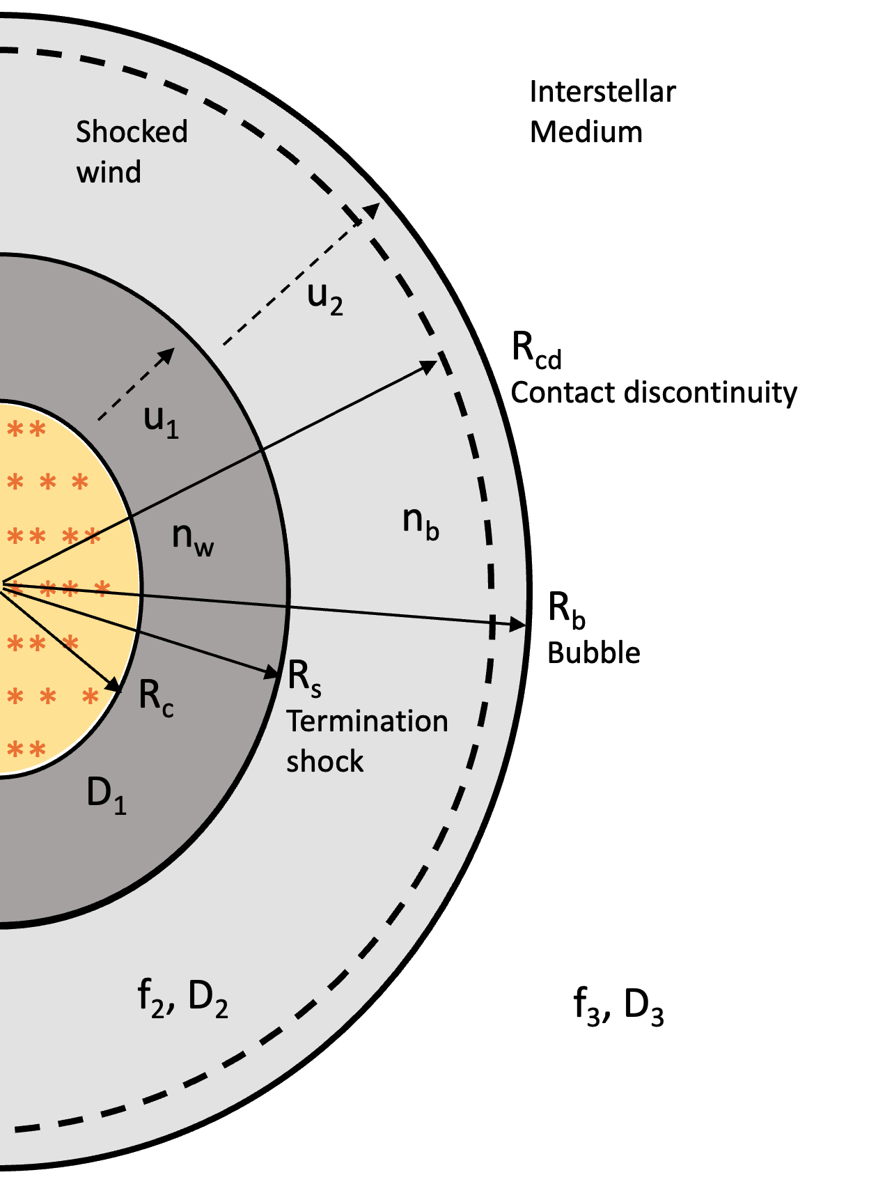
Figure 1: Schematic model for a stellar cluster. CR acceleration occurs at the WTS with radius $R_{s}$, the wind blown bubble extends to a radius $R_{b}$ whilst the member stars of the cluster itself are confined to a radius $R_{c}$. The shocked wind region is indicated by the subscript $2$ whilst the ISM is denoted by the subscript $3$.

2 The wind-blown bubble structure

During the first few Myrs, when no SN has exploded yet, the circumstellar medium around SCs is shaped by stellar winds, which inflate a low density bubble producing a forward shock, expanding into the interstellar medium (ISM), and a reverse shock, i.e. the WTS, expanding into the cold fast wind. The latter is the only one with a Mach number $\gg 1$ and hence is a possible location for particle acceleration (Gupta et al., 2020). We describe the structure of the wind-blown bubble following the stellar analogue by (Weaver et al., 1977). In particular, the location of the WTS is affected by the surrounding density, as well as by the cluster age and properties of member stars, e.g. their mass loss rate and wind velocity (that combine into kinetic luminosity). A schematic representation of the wind-driven bubble is provided in Fig. 1, showing both the forward shock of the wind blown bubble at distance $R_{b}$ and the WTS at distance $R_{s}$ equal to

$$R_{\rm s}(t)= 26\,\left(\frac{\dot{M}_{\rm c}}{10^{-4}\mathrm{M}_{\odot}\mathrm{yr}^{-1}}\right)^{3/10}\left(\frac{v_{\rm w}}{2000\,\mathrm{km\,s}^{-1}}\right)^{1/10}$$ (1)

$$\times\left(\frac{n_{0}}{10\,\mathrm{cm}^{-3}}\right)^{-3/10}\left(\frac{t}{10\,\mathrm{Myr}}\right)^{2/5}\,\mathrm{pc}$$

and

$$R_{\rm b}(t)=112\,\left(\frac{L_{\rm w,c}}{10^{37}\,\mathrm{erg\,s}^{-1}}\right)^{1/5}\left(\frac{n_{0}}{10\,\mathrm{cm}^{-3}}\right)^{-1/5}\left(\frac{t}{10\,\mathrm{Myr}}\right)^{3/5}\mathrm{pc}$$ (2)

with cluster age $t$, number density of the ISM outside of the wind bubble $n_{0}$, SC mass loss rate $\dot{M}_{\rm c}$, its wind velocity $v_{\rm w}$ and its wind luminosity $L_{\rm w}=\frac{1}{2}\dot{M}_{\rm c}v_{\rm w}^{2}$. The parameters determining the energy output of a stellar cluster can be obtained from the characterization of its stellar population.

In Celli et al. (2023) we developed a method to infer the stellar mass distribution of each cluster that reproduces the observed number of member stars per cluster by Gaia (Cantat-Gaudin et al., 2020). Our procedure accounted for both bolometric correction and light extinction from each individual cluster direction to derive the correct normalization of the stellar mass function, assumed in the form of a Kroupa distribution (Weidner & Kroupa, 2004). As such, we could extend the mass domain of our investigation beyond Gaia observations, by including all stellar masses between $0.08\,M_{\odot}$ and the maximum stellar mass expected to still exist in the cluster in its main sequence phase. The latter was determined by theoretical considerations as either limited by cluster age, $M^{*}_{\rm max}(t_{\rm age})$, or by the parent cluster mass, $M^{*}_{\rm max,0}$. We obtained reasonable cluster mass values (namely within a factor 2 of literature estimations), which we find acceptable given the intrinsic limitations of our procedure, that strongly relies on individual star detection inside SCs. These are known to be affected by many source of uncertainties: for example, spatial resolution might become insufficient in dense regions as the cluster cores; massive stars might occur in binary systems; star membership to clusters might also suffer identification problems (see Celli et al., 2023, for a more detailed discussion on the mass uncertainty). Once the stellar population is determined for each SC, we determine the SC wind mass loss rate and velocity starting from the properties of each stellar wind.

We focus on young SCs from this Gaia DR2 sample, namely those with age smaller than 30 Myr. From the cluster wind mass loss rate and wind velocity, we can derive the cluster wind luminosity required to model the SC particle acceleration. The resulting distribution of $R_{\rm s}$ and $R_{\rm b}$ in our SC sample is shown in Figure 2, with $R_{\rm s}$ and $R_{\rm b}$ peaking at $\sim 2$ pc and $\sim 45$ pc respectively.

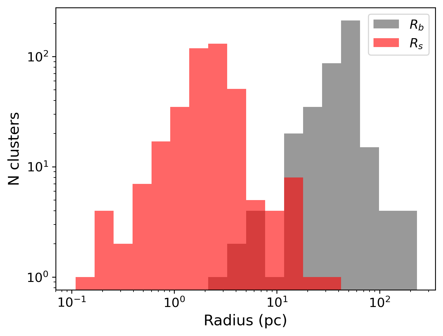
Figure 2: Distribution of wind termination shock $R_{s}$ and bubble radii $R_{b}$ evaluated from Eqs. (1) and (2) for our sample of stellar clusters.

The density profile of target gas inside of the bubble follows from the description of Weaver et al. (1977). Within the cluster core, we assume for simplicity a constant value, fixed by a continuity condition with the cold wind profile at the cluster core $R_{\rm c}$, namely

$$n_{\rm c}=\frac{\dot{M_{\rm c}}}{4\pi R^{2}_{\rm c}v_{w}}\qquad r<R_{\rm c}$$ (3)

where for $R_{\rm c}$ we adopt the $R50$ value from Cantat-Gaudin et al. (2020) which is the radius that contains half of the cluster members. This angular size is converted into a physical size using the cluster distance, either as reported in the same catalogue, or from the updated Gaia DR3 where available. The model scenario for a wind-blown bubble around a stellar cluster is only valid for compact clusters. For the cases where $R_{\rm c}$ is found to be larger than the termination shock radius (1) it is not clear whether a WTS can be formed, hence our acceleration model cannot be applied. Therefore, those clusters are removed from our sample, leaving $\sim 140$ young, compact stellar clusters.

Within the cold wind region, the ambient density profile is expected to drop as $\propto r^{-2}$, where the density of material is determined by the mass loss rate:

$$n_{\rm w}(r)=\frac{\dot{M_{\rm c}}}{4\pi r^{2}v_{\rm w}}\qquad R_{\rm c}\leq r<R_{\rm s}$$ (4)

In the hot wind region, namely between $R_{\rm s}$ and the contact discontinuity located at $r=R_{\rm cd}$, the density profile is constant again but determined by both the mass injected by the wind and by the mass evaporation from the outer shell, whose rate evolves as (Menchiari, 2023):

$$\dot{M}_{\rm sh}=2\times 10^{-4}\left(\frac{L_{\rm w,c}}{10^{37}\,{\rm erg/s}}\right)^{\frac{27}{35}}\left(\frac{n}{10\,{\rm cm}^{-3}}\right)^{-\frac{2}{35}}\left(\frac{T_{\rm age}}{1\,{\rm Myr}}\right)^{\frac{6}{35}}\,M_{\odot}\,{\rm yr}^{-1}\,,$$ (5)

such that the total mass present within the bubble depends on the cluster wind luminosity. Given its weak dependence on time, we treated the mass evaporation rate as constant and computed the amount of evaporated mass from the shell as $M_{\rm sh}=\dot{M}_{\rm sh}(t_{\rm age})t_{\rm age}$. This mass will contribute to the mass contained in the shocked wind region, in addition to the mass flow from the wind, that can be estimated as $\dot{M}_{\rm w}T_{\rm age}-\dot{M}_{\rm w}/(v_{\rm w}(R_{\rm s}-R_{\rm c}))$, the two terms representing the total mass ejected during the cluster lifetime and the mass going into the cold wind, respectively, in order to guarantee mass conservation. An additional contribution to the bubble mass comes from the ejecta of all supernova (SN) explosions occurred during the cluster lifetime, $N_{\rm sn}$, that we compute from the stellar mass function $\xi(M)$ as:

$$N_{\rm sn}(t_{\rm age})=\int_{M^{*}_{\rm min}}^{M^{*}_{\rm max,0}}\xi(M)dM$$ (6)

where $M^{*}_{\rm min}=\min[8\,M_{\odot},M^{*}_{\rm max}(t_{\rm age})]$. In other words, the total mass in the hot wind reads as

$$M_{\rm b}=(\dot{M}_{\rm sh}+\dot{M}_{\rm w})\,t_{\rm age}-\frac{\dot{M}_{\rm w}}{v_{\rm w}(R_{\rm s}-R_{\rm c})}+N_{\rm sn}(t_{\rm age})M_{\rm ej}$$ (7)

where $M_{\rm ej}$ represents the ejecta mass for a single supernova, that we set to 5 $M_{\odot}$. We hence obtain the number density $n_{\rm b}$ in the bubble as:

$$n_{\rm b}=\frac{M_{\rm b}}{\frac{4}{3}\pi\left(R^{3}_{\rm cd}-R^{3}_{\rm s}\right)m_{\rm p}}\leavevmode\nobreak\ ,$$ (8)

Finally, the density in the shell is simply determined by the compressed ISM density, corresponding to the entire amount of swept-up mass, depleted by the evaporated shell mass (5) as:

$$n_{\rm sh}=\frac{n_{0}}{1-R^{3}_{\rm cd}/R^{3}_{\rm b}}-\frac{\dot{M}_{\rm sh}t_{\rm age}}{m_{\rm p}V_{\rm sh}}\leavevmode\nobreak\ ,$$ (9)

where $V_{\rm sh}$ is the volume of the shell between the contact discontinuity radius $R_{\rm cd}\simeq 0.95R_{\rm b}$ and the bubble radius $R_{\rm b}$.

2.1 The fragmented shell scenario

The model by (Weaver et al., 1977) contains two important approximations: first the radiative losses are neglected and, second, the shell of swept up material is assumed to be spherical. Numerical simulations have shown that the shell usually fragments as a consequence of different kind of hydrodynamical (HD) instabilities, resulting in a complex fractal structure of filaments and clumps (Lancaster et al., 2021a, b). The impact of such a process onto the bubble evolution is not completely understood, partly because simulations usually neglect the role of magnetic field that typically suppresses HD instabilities. The consequence of fragmentation is that the gas target density inside the bubble increases, resulting into a larger $\gamma$-ray flux and a harder spectrum. Some level of fragmentation is indeed required in the case of the Cygnus cocoon if one wants to explain the $\gamma$-ray emission as due to hadronic interactions (Menchiari et al., 2024; Blasi & Morlino, 2023). At the moment, the uncertainties in the fragmentation process are such that is it unclear how to treat this phenomenon realistically. Here we try to account for such a process, making the simplifying assumption that a fraction $\eta_{\rm fr}\approx 10\%$ of the shell material fragments into dense clumps that uniformly fill the bubble structure. In such a scenario, the shell density decreases by $\eta_{\rm fr}$ while the bubble density increases, i.e.

$$n_{\rm sh}^{\prime} =(1-\eta_{\rm fr})\,n_{\rm sh}$$

$$n_{b}^{\prime} =n_{b}+\eta_{\rm fr}\,n_{\rm sh}\,R_{\rm b}^{3}/R_{\rm cd}^{3}=n_{\rm b}+0.0116\,\left(\frac{\eta_{\rm fr}}{0.1}\right)\,n_{0}$$ (10)

where $n_{\rm sh}$ is given by Eq. (9) and $n_{\rm b}$ by Eq. (8). Henceforth, we will distinguish the baseline scenario from the fragmented shell scenario. In the baseline scenario, the contribution coming from the shell easily dominates over the bubble term in Eq. (8) but, when the shell fragments, the two contribution may become comparable. A representation of the expected density profile with and without fragmentation is reported in Figure 3(a) using $\eta_{\rm fr}=10\%$. One should keep in mind, however, that the fragmentation fraction of 10% may be underestimated.

3 Non-thermal particle production in stellar clusters

We assume that particles are accelerated by two different processes; a continuous acceleration occurring at the WTS and impulsive acceleration from SNR shocks. The former dominates during the first $\sim 3$ Myrs before the first SN explosions start taking place. Because the average time between two SN explosions is usually $\gtrsim 10^{5}$ yr, we assume that the WTS gets formed again to keep accelerating particles between different SN events.

3.1 Contribution from the wind termination shock

For particle acceleration at the WTS, we use the model developed by Morlino et al. (2021). The authors solved the spherically symmetric transport equation of particles within the environment of a SC to obtain a relation for the spectrum of accelerated particles $f(r,p)$ as a function of the particle momentum $p$ and the distance to the SC centre $r$. In our work, we will refer to quantities in the cold wind region with subscript 1 ($r<R_{s}$), inside the shocked wind with subscript 2 ($R_{s}<r<R_{b}$) and outside of the wind blown bubble with subscript 3 ($r>R_{b}$), see Figure 1. With this nomenclature, the particle distribution function in the shocked wind region $f_{2}(r,p)$ can be written as:

$$f_{2}(r,p)= f_{s}(p)\mathrm{e}^{\alpha(r)}\frac{1+\beta(\mathrm{e}^{\alpha(R_{b})}\mathrm{e}^{-\alpha(r)}-1)}{1+\beta(\mathrm{e}^{\alpha(R_{b})}-1)}$$ (11)

$$+f_{\mathrm{Gal}}(p)\frac{\beta\left(\mathrm{e}^{\alpha(r)}-1\right)}{1+\beta(\mathrm{e}^{\alpha(R_{b})}-1)}$$

while that outside the wind blown bubble $f_{3}(r,p)$ is

$$f_{3}(r,p)=f_{b}(p)\frac{R_{b}}{r}+f_{\mathrm{Gal}}(p)\left(1-\frac{R_{b}}{r}\right)$$ (12)

where $f_{b}(p)=f_{2}(R_{b},p)$ is the particle distribution at the bubble boundary, and $f_{s}(p)$ is the one at the WTS:

$$f_{s}(p)=\frac{3\,\xi_{\mathrm{CR}}\,n_{1}u_{1}^{2}}{4\pi\Lambda(m_{p}c)^{3}c^{2}}\left(\frac{p}{m_{p}c}\right)^{-s_{\rm wts}}\mathrm{e}^{-\Gamma(p)}\,.$$ (13)

Far away from the bubble, the CR spectrum reduces to the average sea of Galactic CR $f_{\mathrm{Gal}}(p)$, which is assumed to be the same as that measured close to Earth (Aguilar et al., 2015). In the latter expression (13), $\xi_{\mathrm{CR}}$ is the acceleration efficiency expressed as the fraction of incoming momentum flux converted into CR pressure, i.e. $P_{\rm cr}=\xi_{\rm cr}\,\rho_{1}u_{1}^{2}$. The normalization factor is $\Lambda=\int_{x_{\rm inj}}^{\infty}x^{4-s_{\rm wts}}\mathrm{e}^{-\Gamma(x)dx}$, while $s_{\rm wts}=3u_{1}/(u_{1}-u_{2})$ is the slope. In general for strong shock $s_{\rm wts}\simeq 4.0$, such that $\Lambda\simeq\ln\frac{p_{\max,1}}{m_{p}c}$. Larger values of $s_{\rm wts}$ can be obtained when magnetic field amplification effects are accounted for (see discussion in Morlino et al., 2021); however, here we neglect these additional effects. Finally, the functions $\alpha$ and $\beta$ are:

$$\alpha(r,p) = \frac{u_{2}R_{s}}{D_{2}(p)}\left(1-\frac{R_{s}}{r}\right)$$ (14)

$$\beta(p) = \frac{D_{3}(p)R_{b}}{u_{2}R_{s}^{2}}$$ (15)

where the diffusion coefficients are assumed to be spatially constant within each of the regions: $D_{2}$ in the shocked wind and $D_{3}$ in the ISM. Finally, the cutoff term, $e^{-\Gamma(p)}$, depends on the maximum energy and has an involved expression that hides the non-linearity of the solution. However, it can be adequately approximated by the following expression:

$$\mathrm{e}^{-\Gamma(p)}\simeq\left[1+a_{1}\left(\frac{p}{p_{\mathrm{max,1}}}\right)^{a_{2}}\right]\,\exp\left[-a_{3}\left(\frac{p}{p_{\mathrm{max,1}}}\right)^{a_{4}}\right]\leavevmode\nobreak\ ,$$ (16)

where the values of the $a_{i}$ parameters depend on the diffusion scenario adopted, and are provided below.

In the model by Morlino et al. (2021), the cluster wind velocity is assumed to be constant in the cold wind region $u_{1}$, compressed when passing the TS to $u_{2}=u_{1}/\sigma$ with compression factor $\sigma$ (typically $\sigma=4$) and decreasing with radial distance to the cluster centre as $\propto r^{-2}$ in the shocked wind region, hence:

$$u(r)=\cases{u}_{1}&r<R_{s}\\ u_{2}\left(\frac{R_{s}}{r}\right)^{2}R_{s}<r<R_{b}\\ 0r>R_{b}\,.{}$$ (17)

In the light of recent results on diffusion properties inside the wind blown bubble around Cygnus OB2 (Blasi & Morlino, 2023; Menchiari et al., 2024), magnetic turbulence inside SC wind bubbles is assumed to be dominated by Kraichnan scaling with diffusion coefficient following

$$D_{\rm Kra}(p,B)=\frac{c}{3}\sqrt{r_{L}(p,B)\,L_{\mathrm{coh}}}$$ (18)

with particle momentum $p$, magnetic field strength $B$, coherence scale of the magnetic field in the shocked wind region $L_{\mathrm{coh}}$ and particle Larmor radius

$$r_{L}(p,B)=\frac{pc}{eB}$$ (19)

with elementary charge $e$. However, we emphasize that detailed knowledge on diffusion properties inside SC wind bubbles is still very limited. We will show below that in some cases the Bohm diffusion seems to be more consistent with some observed $\gamma$-ray spectra. In such a case the diffusion coefficient is $D_{\rm Bohm}=r_{L}(p,B)\,c/3$. In the scenario of Kraichnan diffusion, the parameters used in Eq.(16) are $a_{1}=5$, $a_{2}=0.449$, $a_{3}=12.52$, , $a_{4}=0.643$, while for Bohm $a_{1}=8.94$, $a_{2}=1.296$, $a_{3}=5.310$, $a_{4}=1.132$ (Menchiari et al., 2024).

Note that in this model $p_{\max,1}$ is the maximum momentum obtained from the confinement condition in the upstream region, i.e. $D_{1}/u_{1}<R_{s}$, however it does not represent the effective maximum momentum, which is also affected by the escaping condition in the downstream and is accounted for in the shape of the cutoff in Eq. (16). The magnetic field in the unshocked wind region is computed assuming that a fraction $\xi_{B}$ of the wind kinetic luminosity is converted into magnetic energy flux:

$$B(r)=\frac{1}{r}\sqrt{\frac{\xi_{B}}{2}\dot{M}u_{1}}$$ (20)

while in the shocked wind region the magnetic field is assumed to be stronger by a factor $\sqrt{11}$ due to compression at the WTS. Benchmark values for $\xi_{\mathrm{CR}}$, $\xi_{\mathrm{B}}$, $L_{\mathrm{coh}}$ and $\sigma$ assumed in this work are listed in Table 1, unless differently specified. Typical values of $B$ obtained in the shocked wind region are $\approx(2-16)\mu$G for wind luminosity in the range $\sim 10^{34}-10^{38}$ erg s^-1.

3.2 Contribution from SNRs inside SCs

In addition to CRs accelerated at the WTS, SCs older than $\approx 3$ Myr are expected to be populated by non-thermal particles produced at SNR shocks. A full and consistent treatment of this scenario is not easy to achieve for several reasons. First of all, SN explosions inject energy on a timescale much smaller than the cluster age, hence the bubble structure is probably modified in a non stationary way, producing transient phases. Moreover and more importantly, the evolution of a SNR shock inside the bubble itself is complicated by the non homogeneity of the medium: the presence of stellar winds and termination shocks results in a non smooth evolution of the SNR shock and may produce multiple reflected shocks (Dwarkadas, 2005, 2007). As a consequence, a correct description of particle acceleration requires a time dependent calculation. Moreover, particle acceleration is strongly affected by the conditions of the plasma inside of the bubble where the shock expands, especially by the magnetic field configuration, which, as stressed above, is quite uncertain. In spite of all these complications, here we give an approximate estimate of the SNR contribution to the SC $\gamma$-ray emission, making several simplifying assumptions. In particular, we will consider the bubble size to be determined by the stellar winds only, and its density to be homogeneous. Vieu & Reville (2023) consider a similar scenario, but distinguish between compact and loose clusters, showing that the former are more promising in producing PeV particles in that the magnetic field is pre-amplified by the MHD turbulence generated by the WTS. We follow a similar reasoning however, as shown below, we obtain maximum energies in general smaller than those predicted by Vieu & Reville (2023) because the magnetic field strength estimated for the SCs in our sample is smaller.

We first note that when a SN explodes, it initially expands inside the cold fast wind until it reaches the WTS and then proceeds through the hot bubble. Because the mass enclosed in the cold wind is usually much smaller than the mass of the ejecta, the SN kinetic energy is mainly released in the hot bubble. Hence we approximate the SNR evolution as if it were expanding only inside the hot bubble with uniform density, $n_{\rm b}$. We can approximate the SNR evolution mainly in two phases: the ejecta dominated (ED) phase, when the swept-up mass is smaller than the ejecta mass, and the Sedov-Taylor phase, when $M_{\rm swept-up}>M_{\rm ej}$. During the ED phase the shock speed is roughly constant and is given by $u_{\rm st}=(2E_{\rm sn}/M_{\rm ej})^{1/2}$, where $E_{\rm sn}$ and $M_{\rm ej}$ are the explosion energy and ejecta mass, respectively. The ED phase lasts a time $t_{\rm st}=R_{\rm st}/u_{\rm st}$ where the radius $R_{\rm st}$ is determined by the condition that $M_{\rm swept-up}=M_{\rm ej}$, hence $R_{\rm st}=[3M_{\rm ej}/(4\pi n_{\rm b}m_{\rm p})]^{1/3}$, $m_{\rm p}$ being the proton mass. On the contrary, during the ST phase, the shock’s radius and velocity scale as $R_{\rm sh}=R_{\rm st}(t/t_{\rm st})^{2/5}$ and $u_{\rm sh}=dR_{\rm sh}/dt=(2/5)\,R_{\rm sh}(t)t$. As we show below, the amount of accelerated particles during the two phases is roughly the same.

For a constant shock speed, the CR distribution at the shock is given by the usual power-law with exponential cutoff

$$f_{\rm snr}(p)=\frac{3\xi_{\rm cr}n_{b}u_{\rm sh}^{2}}{4\pi\,\Lambda(m_{p}c)^{4}c^{2}}\left(\frac{p}{m_{p}c}\right)^{-s_{\rm sn}}\mathrm{e}^{-p/p_{\max}}\,.$$ (21)

Eq. (21) is identical to Eq.(13) with the exception of the exponential term which contains a different maximum momentum that will be defined below. Also, note that the numerical value of the slope $s_{\rm sn}$ can be different from the $s_{\rm wts}$ that appears in Eq.(13). The amount of CRs produced by a single SNR during the ED phase is

$$F_{\rm snr}(t<t_{\rm st})=\int_{0}^{t_{\rm st}}f_{\rm snr}(p)\frac{u_{\rm sh}}{4}\,4\pi R_{\rm sh}^{2}dt=\frac{\pi}{3}\,R_{\rm st}^{3}\,f_{\rm snr}(p)$$ (22)

where $u_{\rm sh}/4=u_{\rm st}/4$ is the downstream speed and we have used $u_{\rm st}dt=dR_{\rm sh}$. When performing the same estimation during the ST phase up to the beginning of the radiative phase, $t_{\rm rad}$, we obtain

$$F_{\rm snr}(t>t_{\rm st})=3\left(\frac{2}{5}\right)^{3}\ln\left(\frac{t_{\rm rad}}{t_{\rm st}}\right)\,F_{\rm snr}(t<t_{\rm st})\,.$$ (23)

Typically $t_{\rm rad}\approx 50\,t_{\rm st}$, hence the ratio between the two contributions is $F_{\rm snr}(t>t_{\rm st})/F_{\rm snr}(t<t_{\rm st})\approx 0.75$. However, during the ST phase, the maximum energy decreases in time, hence we only consider the contribution produced during the ED phase.

On the million year long timescale of evolution of clusters, the particles produced by a single SNR will escape the bubble because of both diffusion and advection. Hence the CR distribution is contributed by all the SNe exploded during an escape time, $N_{\rm sn}(t_{\rm esc})$. We set this escape time to be equal to the advection time in the bubble, namely $t_{\rm esc}\approx t_{\rm adv}=\int_{R_{s}}^{R_{b}}dr/u(r)\simeq 0.6t_{\rm age}$. The average distribution over the bubble volume will then be

$$\langle f_{\rm snr}\rangle=N_{\rm sn}(t_{\rm esc})\frac{F_{\rm snr}}{V_{\rm bubble}}=N_{\rm sn}(t_{\rm esc})\,\frac{\xi_{\rm cr}n_{b}u_{\rm st}^{2}}{4}\,\frac{R_{\rm st}^{3}}{R_{b}^{3}}\,.$$ (24)

It is convenient to evaluate the ratio between CRs produced by SNRs and those produced by the WTS at a specific particle momentum:

$$\mathcal{R} \equiv\left.\frac{\langle f_{\rm snr}\rangle}{f_{\rm ts}}\right|_{p=m_{p}c}=\frac{n_{b}u_{\rm st}^{2}}{n_{w,1}u_{w}^{2}}\frac{R_{\rm st}^{3}}{R_{\rm b}^{3}}\frac{N_{\rm sn}(t_{\rm esc})}{4}=1.65\,\frac{N_{\rm sn}E_{\rm sn}}{L_{w}t_{\rm adv}}$$

$$=1.74\,N_{\rm sn}(t_{\rm esc})\left(\frac{E_{\rm sn}}{10^{51}\,\rm erg}\right)\left(\frac{L_{w}}{10^{37}\rm erg\,s^{-1}}\right)^{-1}\left(\frac{t_{\rm age}}{\rm 3\,Myr}\right)^{-1}$$ (25)

such that Eq.(24) can be rewritten as

$$\langle f_{\rm snr}(p)\rangle=\mathcal{R}\,f_{\rm ts}(m_{p}c)\,\left(\frac{p}{m_{p}c}\right)^{-s_{\rm snr}}\mathrm{e}^{-p/p_{\max}}\,.$$ (26)

Note that in Eq. (3.2) we used $R_{\rm b}$ from Eq. (2) and assumed that the acceleration efficiency is the same for both types of shocks. Not surprisingly, the ratio $\mathcal{R}$ depends solely on the energy input of SNe and stellar winds.

Now, we should evaluate the maximum energy of particles accelerated at SNRs, representing the most uncertain part of the calculation due to the lack of knowledge about the magnetic turbulence development inside the bubble. To this extent, we adopt the time-limited condition by equating the acceleration time, $t_{\rm acc}\simeq 8D/u_{\rm st}^{2}$ with the beginning of the ST age, $t_{\rm st}$. Writing as usual, the diffusion coefficient as $D=r_{L}c/(3\mathcal{F})$, we get

$$E_{\max}=41\,\mathcal{F}\left(\frac{B}{\mu G}\right)\left(\frac{E_{\rm sn}}{10^{51}\rm erg}\right)^{\frac{1}{2}}\left(\frac{M_{\rm ej}}{5\rm M_{\odot}}\right)^{-\frac{1}{6}}\left(\frac{n_{b}}{0.1\rm\,cm^{-3}}\right)^{-\frac{1}{3}}\,\rm TeV,$$ (27)

where $\mathcal{F}$ is the logarithmic power spectrum of the magnetic turbulence. If we use solely the diffusion determined by the wind turbulence, i.e. Eq. (18), the maximum energy is rather small:

$$E_{\max}=1\,\left(\frac{B}{\mu G}\right)\left(\frac{E_{\rm sn}}{10^{51}\rm erg}\right)\left(\frac{M_{\rm ej}}{5\rm M_{\odot}}\right)^{-\frac{1}{3}}\left(\frac{n_{b}}{0.1\rm\,cm^{-3}}\right)^{-\frac{2}{3}}\,\rm TeV\,.$$ (28)

On the other hand, the magnetic turbulence may be further enhance by the CR streaming instability through either resonant or non-resonant modes. The latter dominates over the former only when the shock speed and the upstream density are both very large ($u_{\rm sh}\gtrsim 5000\,\rm km/s$ and $n\gtrsim 10\,\rm cm^{-3}$), conditions that are typically realized during the first hundred years of the SNR evolution (Bell et al., 2013). Because such a phase is not described here with accuracy, we will only consider the resonant mode. During the ED phase, the resonant SI is strong enough that $\mathcal{F}\approx 1$, hence we should use the expression for the saturation in the non linear regime (Blasi, 2013), i.e.

$$\mathcal{F}_{\rm res}=\left(\frac{\pi\,\xi_{\rm cr}\,c}{6\,\Lambda\,u_{\rm sh}}\right)^{1/2}=0.5\,\left(\frac{\xi_{\rm cr}}{0.1}\right)^{\frac{1}{2}}\left(\frac{E_{\rm sn}}{10^{51}\rm erg}\right)^{\frac{1}{4}}\left(\frac{M_{\rm ej}}{5M_{\odot}}\right)^{-\frac{1}{4}}$$ (29)

With such a value of $\mathcal{F}$ and assuming $B\simeq 10\,\mu$G, the maximum energy in Eq.(27) can achieve $\sim 200$ TeV. Note that, in this approach, the maximum energies achieved at SNR shock and at the WTS are not independent quantities but are connected through the value of the magnetic field in the bubble (see Fig. 5 and related discussion in Sec. 5.1). Vieu & Reville (2023) performed a similar calculation for the SNR maximum energy but estimated values roughly one order of magnitude larger due to the magnetic field strength which is assumed to reach hundreds of $\mu$G.

4 Secondary particle production in hadronic collisions

Proton-proton collisions result into the production of secondary particles, including neutral and stable messengers such as $\gamma$-rays and neutrinos, that can hence be used as astronomical probes for the occurrence of such interactions. Given the very mild energy dependence of the cross section, the energy spectrum of final products closely resembles that of primaries (Celli et al., 2020). A formal computation of the emissivity $\psi_{\gamma,\nu}(E_{\gamma},r)$ of secondary particles as a function of space is here performed following the treatment of Kelner et al. (2006):

$$\psi_{\gamma,\nu}(E_{\gamma,\nu},r)=c\,n(r)\int_{E_{\gamma,\nu}}^{\infty}\sigma_{\mathrm{pp}}(E)\,f(E,r)\,K_{\gamma,\nu}\left(\frac{E_{\gamma,\nu}}{E},E\right)\frac{dE}{E}\leavevmode\nobreak\ ,$$ (30)

where $n(r)$ is the number density profile of the target medium that was discussed in Sec. 2, $\sigma_{\mathrm{pp}}$ the total inelastic proton cross section, while $f(E,r)$ is the particle distribution function in energy (i.e. $f(E)dE=f(p)d^{3}p$). The functions describing the production of $\gamma$-rays and neutrinos $K_{\gamma,\nu}(E_{\gamma,\nu}/E,E)$ are also taken from Kelner et al. (2006). As the resulting emissivity is given in ph cm^-3 s^-1 TeV^-1, the particle fluxes on Earth are obtained by integrating over the bubble size and accounting for the cluster distance $d$, such that these can finally be expressed as:

$$F(E_{\gamma,\nu})=\frac{1}{4\pi d^{2}}\int_{0}^{R_{b}}4\pi r^{2}\psi_{\gamma,\nu}(E_{\gamma,\nu},r)\,dr.$$ (31)

Although cluster distance estimates are provided in Cantat-Gaudin et al. (2020), where available we instead adopt distances estimated from the third Gaia data release (DR3) (Hunt & Reffert, 2023).

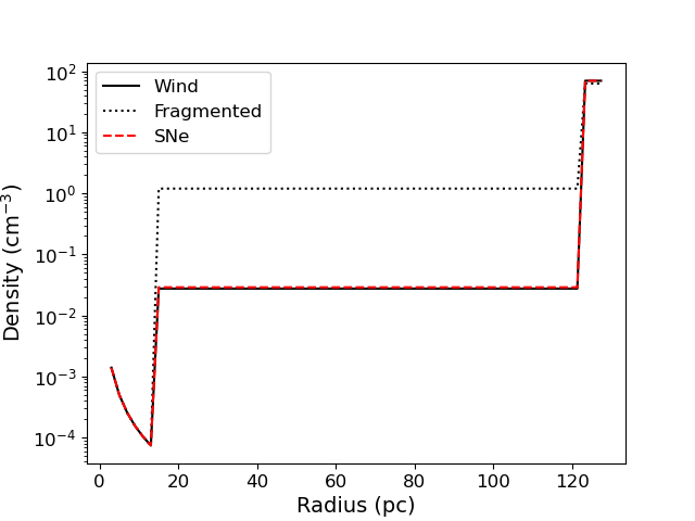
(a)

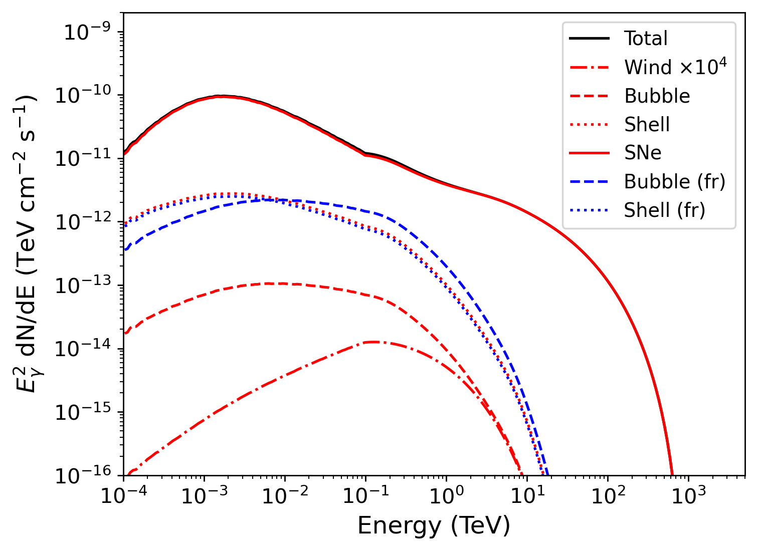
(b)

Figure 3: Left: Density profile in the wind bubble under the different scenarios explored in the text, assuming the benchmark values reported in Table 1. The fragmented shell case assumes $\eta_{\rm fr}=0.1$, while the SNe case accounts for the mass ejected by the 5 SNe occurred during the cluster lifetime, which is negligible compared to the original bubble mass. Right: Predicted $\gamma$-ray emission arising from the different density components of the SC bubble, as discussed in the text; the case of fragmentation leading to a clumpy density distribution is also shown. A representative number of 3 SNe occurred within one advection time is adopted here. Note that we do not include the contribution from Galactic CRs (i.e. $f_{\rm Gal}=0$ in Eq. (11)).

Before applying the model to the sample of Gaia SCs in the next Section, we first discuss some general properties of $\gamma$-ray emission from a typical cluster located at a distance of 1 kpc. When estimating the $\gamma$-ray flux, we set $f_{\rm Gal}$ to zero as we wish to probe the contribution from the SC only. In fact, in $\gamma$-ray data analysis, the contribution due to $f_{\rm Gal}$ is usually removed through the background subtraction methods applied. We adopt representative values for the various cluster-dependent properties as listed in Table 1. Figure 3(b) shows the $\gamma$-ray emission due to accelerated particles emerging from different parts of the system: cold wind, hot bubble and thin shell (red lines). The $\gamma$-ray emission depends primarily on the density of the medium, shown in Figure 3(a), and therefore also on the mass-loss rate of the cluster, as in Eqs. (8) and (9). The average density of the bubble for typical cluster properties is $\sim 0.01$ cm^-3, whilst the density of the surrounding shell of swept up ISM material is $\sim 100$ cm^-3, considerably higher than that of the cold wind region from Eq. (4). Unsurprisingly, the total $\gamma$-ray flux is dominated by the contributions from the shell. However, when one considers the scenario of a fragmented shell, the emission from the bubble can easily become comparable to the one from the shell (blue lines), while the contribution from the free wind region remains unchanged. Figure 3(b) also shows that the contribution from the bubble is harder than the one from the shell, reflecting the fact that the particle distribution function in the bubble is harder at distances closer to the termination shock.

The same Figure also shows the emission due to SNRs (solid red line) assuming that a representative number of 5 SNe occurred along the cluster lifetime, 3 of which during the last advection time. Note that the spectrum due to SNRs is steeper in that we assumed $s_{\rm snr}=4.3$, while for the WTS $s_{\rm wts}=4.0$. The acceleration efficiency is set to 10% for both WTS and SNRs.

The relative contribution between WTS and SNRs is better explored in Figure 4, showing the total differential $\gamma$-ray flux at 1 TeV and 10 TeV as a function of the cluster age: the WTS contribution dominates up to 3 Myr, after which it is overtaken by the SNR one. Notice that the latter is a smooth function because the number of SNe is approximated by the continuous expression provided in Eq. (6), while in reality it will be an integer number for each cluster.

	Parameter	Value
CR	$\xi_{\mathrm{CR}}$	$10\%$
	$\xi_{\mathrm{B}}$	$10\%$
	$L_{\mathrm{coh}}$	$2\,\mathrm{pc}$
	$\sigma$	$4$
	$s_{\rm wts}$	$4.0$
	$\delta$	0.5 (Kraichnan)
	$D_{0}$ (10 GeV)	$3.0\times 10^{28}$ cm2 /s
Cluster	$T_{\rm age}$	3 Myr
	$M_{\rm sc}$	$10^{4}\,M_{\odot}$
	$\dot{M}$	$10^{-5}$ M⊙ /yr
	$v_{w}$	2500  km s-1
	$n_{\rm ISM}$	10 cm-3
	$d$	1 kpc
	$\eta_{\rm fr}$	0.1
SNR	$N_{\rm SN}$	5
	$M_{\rm ej}$	5 $M_{\odot}$
	$E_{\rm sn}$	$10^{51}$ erg
	$s_{\rm sn}$	$4.3$

Table 1: Default parameter values used for the prototype SC model discussed in Sec. 4.

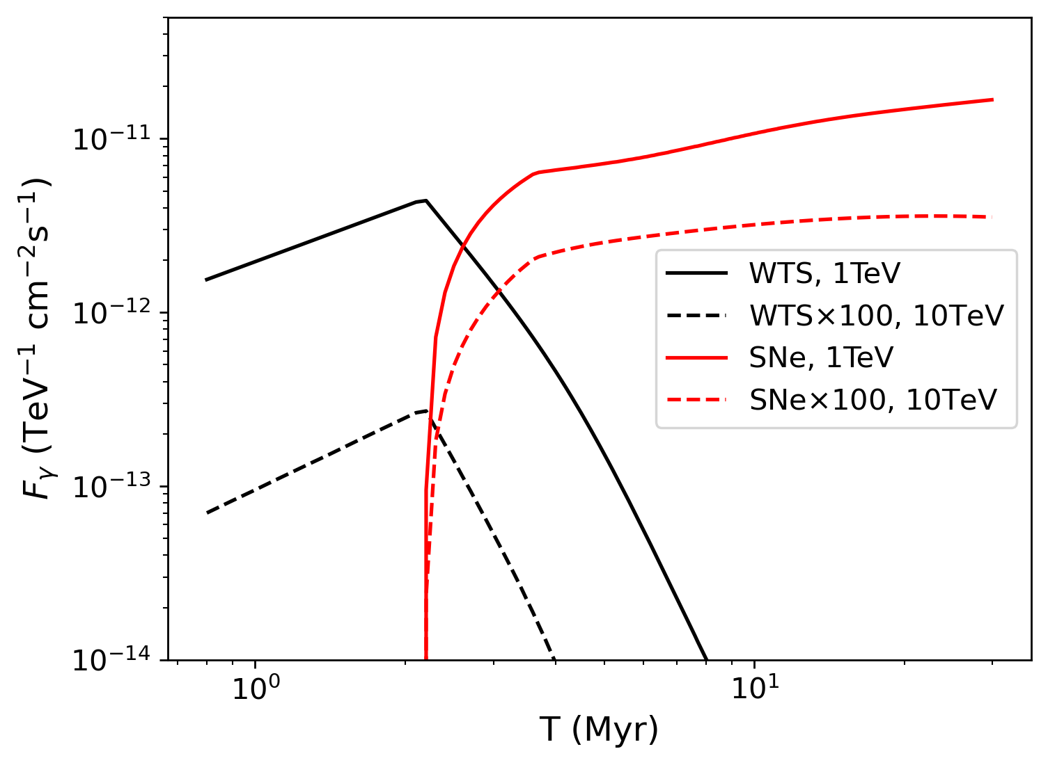
Figure 4: Plot showing the time variation of gamma-ray flux due to particles accelerated at the WTS and from SNRs at 1 TeV and 10 TeV. Note that the latter is multiplied by a factor 100 for ease of visibility.

5 Expected high-energy emission from Young Stellar Clusters from Gaia DR2

We now apply our model to the sample of young stellar clusters from Gaia DR2. In addition to the winds from main sequence stars, we also include a contribution from the associated WR stars reported in the Galactic catalogue (Rosslowe & Crowther, 2015). Our method allows us to characterise the stellar population of each cluster as a function of time and hence to compute the number of stars that have already undergone SN explosions at the SC age. For simplicity, we model this additional contribution to the kinetic luminosity of the system as an injection term at the collective cluster wind, following Sec. 3.2.

5.1 Maximum energy of accelerated particles

Before computing hadronic interactions, we first identify those clusters among the selected sample that most likely result in PeV emission, thereby providing an indication for how many clusters are likely to be PeVatrons. Figure 5 shows the distribution of maximum energies to which CR protons can be accelerated for each SC in our sample as due to the WTS and SNRs. In the case of Kraichnan diffusion, $E_{\max}^{\rm SNR}$ is always larger than $E_{\max}^{\rm WTS}$ except for one cluster, Wd1. With the exception of this case, the maximum energy $E_{\max}^{\rm WTS}$ is always smaller than 1 PeV. The case of Bohm diffusion is more promising, and somehow more extreme, in that 7 SCs are found to have $E_{\max}^{\rm WTS}\geq 1$ PeV (see Table 2).

Notice that the technique applied for the computation of cluster masses relies on the number of stars detected by the Gaia satellite and associated to a cluster using machine-learning techniques. As discussed in Celli et al. (2023), this procedure provides a lower limit to the total SC mass. In particular, in Celli et al. (2023) we quantified an underestimation of SC masses by a factor $\sim 3$ on average. This translates into an equivalent underestimation of the cluster wind luminosity, as well as an underestimation of the maximum energy achieved at the WTS, $E_{\max}^{\rm WTS}$. The latter scales roughly as $\sim L_{\rm w}^{4/5}$ for Kraichnan diffusion and $\sim L_{\rm w}^{1/2}$ for Bohm diffusion (Menchiari et al., 2024), such that we might expect an increase in the estimated WTS maximum energy up to a factor 2.4 and 1.7, respectively. On the other hand, the uncertainty in the SC masses has a milder effect on the maximum energy reached at SNRs, which depends mainly on the magnetic field strength in the bubble (see Eq. (27)): considering that $B_{\rm b}\sim L_{\rm w}^{1/5}$, a factor 3 uncertainty in $L_{\rm w}$ translates into a 25% uncertainty in $E_{\rm max}^{\rm SNR}$. In the next Section, we account for this uncertainty by providing lower and upper bound estimations for the $\gamma$-ray and neutrino emission expected from each SC.

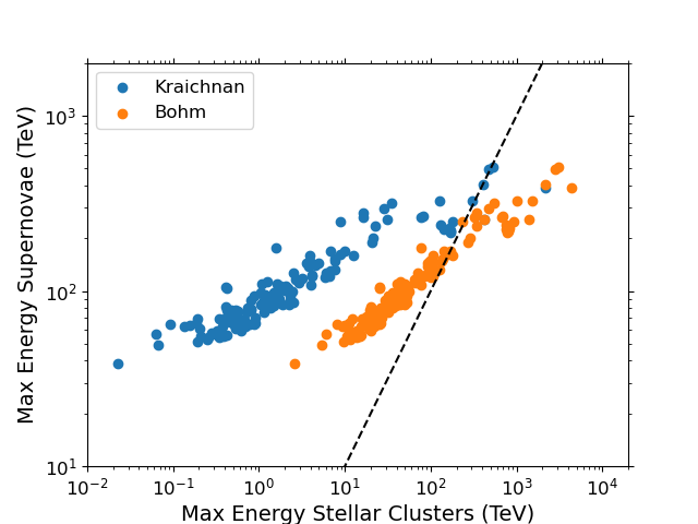
Figure 5: The predicted proton maximum energy from acceleration in the wind for stellar clusters in our sample, compared to the maximum energy due to supernovae assuming Kraichnan or Bohm diffusion in the bubble. The dashed line show the identity $E_{\max}^{\rm SNR}=E_{\max}^{\rm WTS}$.

5.2 Gamma-ray emission

For all of the selected SCs in our sample, we evaluate the expected hadronic $\gamma$-ray emission from the wind-blown bubble. In order to account for the uncertainties in our model, we define minimal and maximal models as follows. In the minimal model, corresponding to our baseline scenario, we only account for particles accelerated at the WTS in the Kraichnan diffusion regime, using the wind luminosity as estimated in (Celli et al., 2023) and the density profile without shell fragmentation. For the maximal model, we instead assume a wind luminosity 3 times larger, to account for the SC mass uncertainty discussed above. In addition, for the maximal model we also include the contribution due to SNRs as well as an increased bubble density due to shell fragmentation. Note that for all models, the acceleration efficiency is fixed to $\xi_{\rm cr}=0.1$ and the ISM density is assumed to be 10 cm^-3, consistent with the fact that these clusters are typically situated in dense environments, surrounded by the Giant Molecular Clouds from which they are born (Menchiari, 2023).

Figure 6 compares the predicted $\gamma$-ray emission from the brightest clusters according to our model to sensitivity curves for current and next-generation ground-based instruments, split according to their visibility from either the Northern or the Southern hemisphere. As shown in Fig. 2, the typical radii of cluster bubbles are of order $\sim 10-100$ pc, which yields a $\sim$degree scale angular size on the sky, with a median bubble radius of $1.6^{\circ}$. As a result, detection prospects for these objects are more realistically evaluated through the comparison with instrument sensitivities with regards to extended sources. For this reason, we report both the point-like and the degraded sensitivity curves of either LHAASO-KM2A and CTA-N (in the North) or CTA-S (in the South), appropriate for bubbles with angular sizes of 0.5 degrees or 1.0 degrees, as calculated in Celli & Peron (2024). For Cherenkov telescopes, on-axis observations are considered. Figure 6 therefore only shows clusters whose angular size (in the baseline scenario) is comparable to the extended sensitivity curves shown, namely $0.25^{\circ}<R_{b}<0.75^{\circ}$ for the left hand panels and $0.75^{\circ}<R_{b}<1.5^{\circ}$ for the right hand ones. The predicted $\gamma$-ray emission for wind-blown bubbles of other angular sizes is not shown in Figure 6. Despite many predicted fluxes being above the point-like sensitivity of current detectors, quite often the degraded sensitivity curve for the corresponding angular size is no longer adequate to suggest that a detection is possible within a comparable observation time. This is well illustrated by the lower right panel of Figure 6, for Southern hemisphere sources with 1.0 degree angular size. Also in Figure 6, the emission is shown for the minimal (solid lines) and maximal models (dashed lines).

Given the strong variation in instrument sensitivity with angular size, in Figure 7 we show the predicted integral $\gamma$-ray flux from the SC bubbles in comparison to the expected CTA-S and CTA-N 100 hour sensitivity at the corresponding angular bubble size. Integral sensitivity lines are obtained following the methods from Celli & Peron (2024) that is based on the official response functions from each detector specifically for on-axis observations. However, for sources with radial extension beyond $2^{\circ}$, a further degradation of the telescope performance should be considered due to off-axis observations. Such a degradation is also energy dependent, e.g. for a source radius of $4^{\circ}$ the worsening with respect to the point-like on-axis case is expected to amount to a factor 4 above 1 TeV (see figure 3 from Celli & Peron, 2024). We neglect this complication here, and simply provide in Fig. 7 the extended source sensitivity without accounting for any off-axis worsening, indicating with a dashed line the angular sizes where we expect this extrapolation to be less reliable. The error bars represent the uncertainty between the minimal and maximal model predictions, affecting both the absolute flux as well as the expected size of the emitting bubble.

Results for the 25 stellar clusters with the highest predicted $\gamma$-ray emission (integrated over the bubble) are listed in ranked order in Tables 3 and 4 for the minimal and maximal models respectively, while Table 2 summarises the physical properties of the same clusters, including the expected WTS and bubble radii, together with the resulting expected angular size of the bubble radius. One should keep in mind that the ranked order in terms of $\gamma$-ray surface brightness will be different due to the variation in angular size of the wind-blown bubbles. The two Tables present the predicted integral $\gamma$-ray energy fluxes above 1 TeV and 10 TeV compared to upper limits from the H.E.S.S. Galactic Plane Survey (H. E. S. S. Collaboration et al., 2018, HGPS) where available. Whilst several of the clusters have predicted fluxes higher than the quoted upper limit, it should be noted that those upper limits correspond to the angular size of the bubble only up to a maximum angular size of $0.6^{\circ}$, the largest size to which the upper limit map provided with H. E. S. S. Collaboration et al. (2018) can be considered valid. By contrast, the majority of the bubble radii are larger than this value ($\sim 1^{\circ}-4^{\circ}$), implying that these upper limits are not constraining over the cluster angular scales. Tables 3 and 4 also provide the predicted differential $\gamma$-ray flux at 7 TeV for comparison to upper limits reported from the 3HWC survey where available (Albert et al., 2020), which are evaluated from the sky maps provided for the nearest fixed angular size, of $0.5^{\circ}$ $1^{\circ}$ or $2^{\circ}$ respectively. None of these latter upper limits are violated by the predicted fluxes.

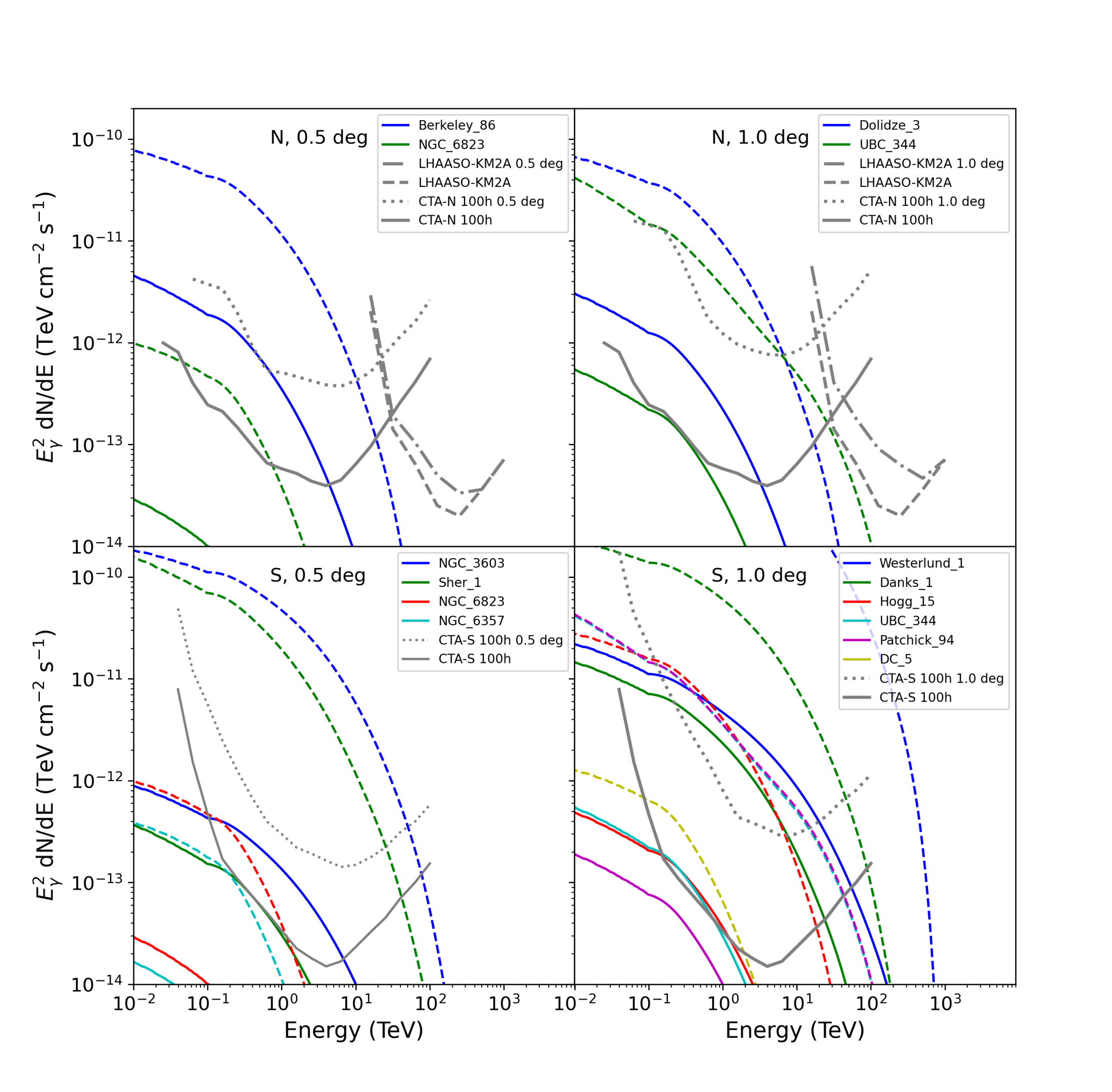
Figure 6: The predicted spectral energy distribution (SED) for $\gamma$-ray emission integrated over the wind-blown bubble, with angular size in the baseline scenario comparable to (i.e. within $0.25^{\circ}$ of) $0.5^{\circ}$ (left panels) and $1.0^{\circ}$ (right panels). Top and bottom panels show the sources visible in the Northern and Southern sky, respectively. Each source is shown with two coloured lines representing the minimal (solid) and maximal (dashed) models. Sensitivity curves for point source and extended sources for CTA-N and CTA-S (at 100 hours exposure) and LHAASO-KM2A (at 1 year exposure) are also shown for reference (grey lines), as taken from Celli & Peron (2024).

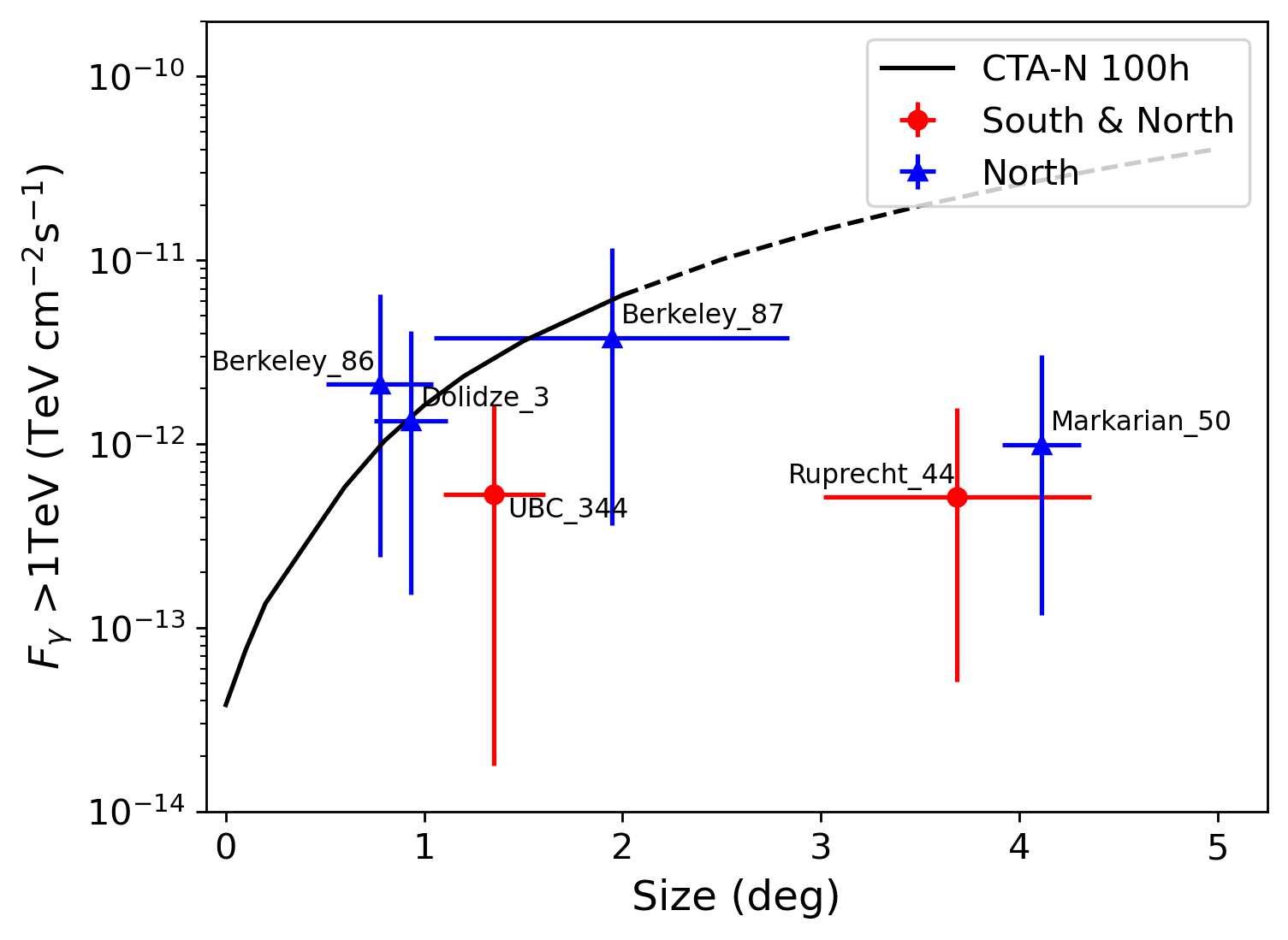
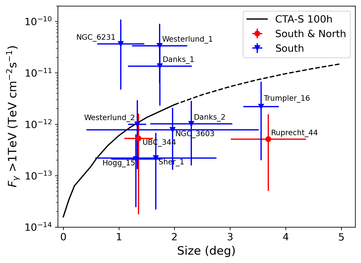
Figure 7: Integral $\gamma$-ray flux above 1 TeV from the cluster bubble, plotted as a function of the bubble size. Top: North and Bottom: South. The sensitivity of the corresponding CTA site for extended sources in 100 h is shown for comparison (Celli & Peron, 2024). The uncertainties show, for each cluster, the minimal and maximal predictions from the model as described in the text.

5.3 Neutrino Emission

For neutrino experiments, the muon neutrino flux is the most relevant astronomical channel, affording good reconstruction prospects in the track-like channel. Due to neutrino oscillations, the muon neutrino flux at Earth is roughly a third of the all-flavour flux, whilst the $\gamma$-rays have a similar normalisation. Therefore, the ranked order of stellar clusters according to the amount of emission produced is unchanged when considering the $\gamma$-ray or the neutrino flux above the same energy threshold. Figure 8 shows the predicted single-flavour muon neutrino SEDs for the brightest clusters, whilst the integral muon neutrino flux values $>10$ TeV are provided in Tables 3 and 4.

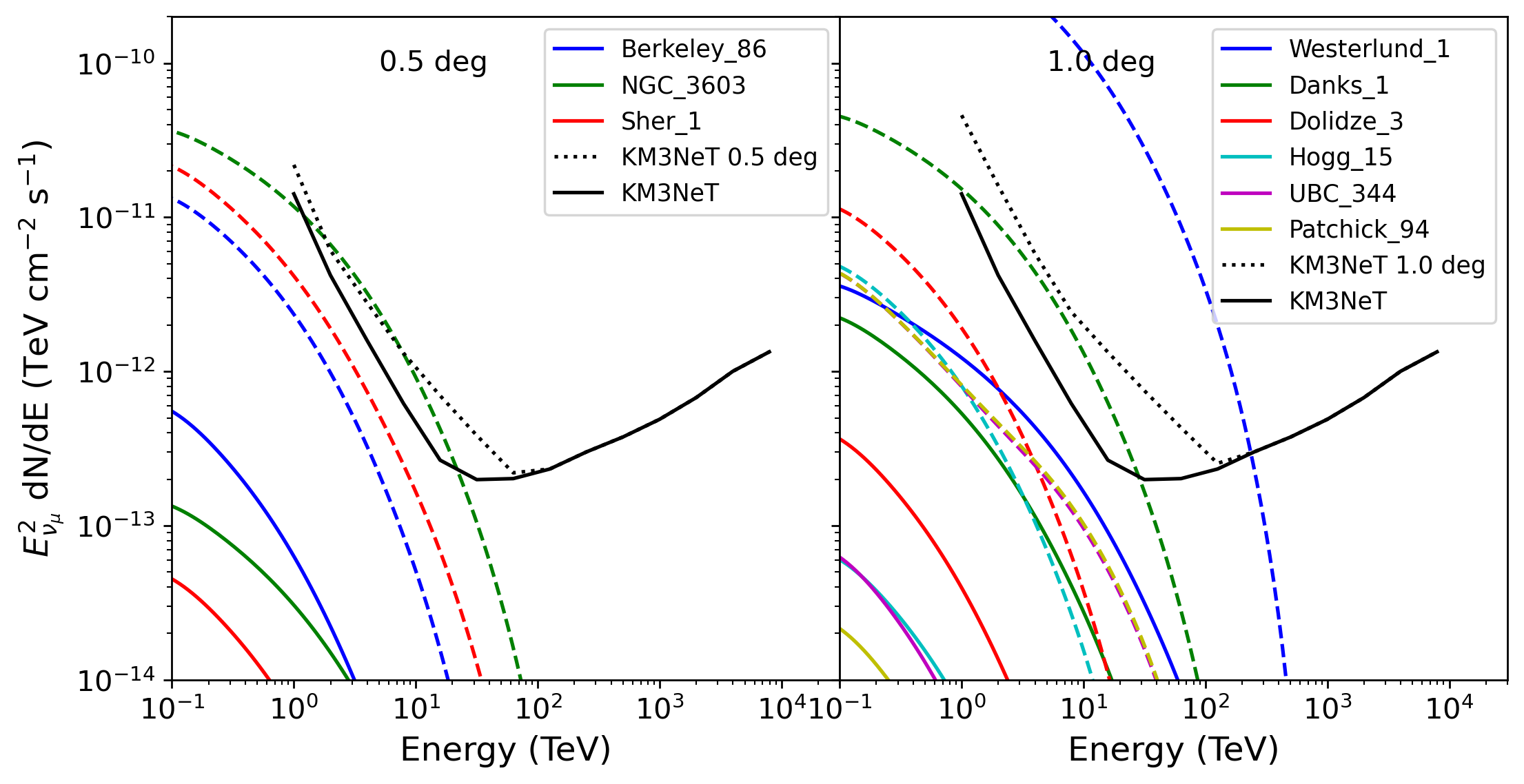
Figure 8: Predicted single-flavour muon neutrino flux from stellar cluster bubbles compared to the KM3NeT sensitivity (at 10 years exposure), under minimal (solid) and maximal (dashed) cases, for angular sizes in the baseline scenario of 0.5 degree (left) and 1.0 degree (right).

Similarly to Figure 6, Figure 8 shows predicted muon neutrino spectral energy distributions (SEDs) compared to the KM3NeT sensitivity curves (at 10 years exposure) for both a point-like source and for a source with an angular extension comparable to 0.5 degrees or 1.0 degrees respectively, as computed in Ambrogi et al. (2018). Only two SCs, NGC 3603 and Westerlund 1 (Wd 1) have a flux above the sensitivity in the maximal model. With regards to Wd1, detection prospects are found to be consistent with the expectations obtained by the KM3NeT Collaboration in the hypothesis of hadronic $\gamma$-ray emission (Unbehaun et al., 2024). A third one, Danks 1, has a flux above the point like sensitivity, but slightly below the degraded sensitivity at 1 degree extension. As such, either solid detection or constraining upper limits are expected to emerge in the near future for these objects, that will allow us to constrain unambiguously their hadronic acceleration efficiency. A large source sample might be accessible by including events from the cascade channel in order to access the entirety of the expected neutrino flux. In this regard KM3NeT appears extremely promising, as shower reconstruction algorithms have been shown to be able to provide an angular resolution below $2^{\circ}$ at energies above 100 TeV (van Eeden, 2024), compatible with and even smaller than the size of most of the SCs investigated here. Proper evaluations of the combined track and shower sensitivities are currently being performed by the KM3NeT Collaboration, so that the improved performances will demand further future investigations in SC searches. Along similar lines, a stacking analysis could be a more suitable approach in searching for neutrino emission from SC wind-blown bubbles, rather than relying on individual systems.

6 Comparison to $\gamma$-ray detected stellar clusters

To date, three stellar clusters in the Gaia DR2 sample have already been detected in GeV and TeV $\gamma$ rays, i.e. Wd1, Wd2 and NGC 3603 (GeV only). For these specific clusters we can hence compare our flux predictions with the corresponding $\gamma$-ray data, as shown in Figure 9. The grey bands show, for each plot, the flux range enclosed between the minimal (i.e. the baseline scenario outlined above) and maximal models. Notice, however, that the latter differ case-by-case, as explained in the following subsections. It is worth stressing that no fitting was performed: the shaded band and model lines in Figure 9 serve to simply illustrate the behaviour of the model and how the range of reasonable parameters compares to data. A detailed modeling of each source is required to better address the validity of the hadronic model by using also other possible information, such as the spatial morphology which is not considered here.

6.1 Westerlund 1

Wd1 has an estimated age and mass of $\sim 8$ Myr and $2.2\times 10^{4}\,\rm M_{\odot}$ (Celli et al., 2023) respectively, and as such a considerable number of SNe have already occurred within it. We estimate a total number of 51 SNe, contributing to the average density within the cluster, among which 28 SNe have occurred within one advection time, thereby contributing to the total mechanical luminosity of the cluster. Notice, however, that the estimate age in literature ranges from $\sim 4$ Myr (Gennaro et al., 2011) to 10 Myr (Navarete et al., 2022). This uncertainty is probably the result of an intrinsic temporal spread of several Myrs for the star-forming process instead of a single monolithic starburst episode scenario, which consequently may yield different ages when using a different sample of stars or different modelling assumptions. If one considers the smaller age value, the number of SNe would be reduced to $\sim 17$ (14 of which in one advection time). We adopt a distance of 7.7 kpc, as listed in the Gaia DR2 catalogue (Gaia Collaboration, 2018), whilst the corresponding bubble radius estimated with our model is $\sim 231$ pc. Although the distance to Westerlund 1 is debated in literature (see, e.g. Rocha et al., 2022), the implied angular size of a $\sim 231$ pc bubble at the 7.7 kpc distance, $\sim 1.2^{\circ}$, is more consistent with the observed $\gamma$-ray emission, despite several estimates preferring distances $\sim 4$ kpc.

The shaded band in the top panel of Figure 9 shows that the observational data from H.E.S.S.(Aharonian et al., 2022) and Fermi-LAT (Ohm et al., 2013) can be well bracketed by our model. Whilst the lower bound corresponds to the cluster wind only, the upper bound is determined by including shell fragmentation, accounting for the contribution from SNe and for an approximate factor 2 underestimation of the total cluster mass (Celli et al., 2023), the latter being obtained by comparing our mass estimate to literature values available for this cluster (Gennaro et al., 2011). The other lines show the SED resulting from accounting for the different effects one at a time. All cases assume Kraichnan diffusion. The ISM density is set to $10\,{\rm cm}^{-3}$ and a CR efficiency of 10% is sufficient to cover the data.

One can see that the highest energy data point measured by H.E.S.S. lies above the shaded band and that the H.E.S.S. spectrum above $\sim 3$ TeV seems slightly harder than our curved models. Such a discrepancy may point towards a harder mass function in the stellar distribution or a harder diffusion coefficient. Notice also that the nominal maximum energy in Wd1 is $E_{\max}^{\rm WTS}\simeq$ PeV, however, the shape of the predicted curves do not show a sharp cutoff at such an energy. This is the consequence of the spherical geometry of the system as discusses in detail by (Morlino et al., 2021).

We find that our hadronic model can account for the $\gamma$-ray emission, whereas Härer et al. (2023) claim a dominant leptonic contribution. The main caveat from Härer et al. (2023) against a hadronic model is the 60 pc size of the emission region, which appears to be smaller than the size of the bubble for the 3.9 kpc distance adopted by Aharonian et al. (2022). Although we estimate a rather larger bubble size, the fragmentation process can be responsible for an apparent reduced size of the bubble, especially if CR are allowed to easily escape from the region where the fragmented shell is located. In fact, the magnetic turbulence may be damped while the plasma is advected away from the termination shock, implying a faster escape of particles and a corresponding reduced $\gamma$-ray emission. Our model does not account for such an effect which we consider important to asses the full validity of the hadronic model.

6.2 Westerlund 2

In the case of Wd2, which has an estimated age of 4 Myr and a mass of $2200\,\rm M_{\odot}$ (Celli et al., 2023), there is only a 50% chance of one SNe having already occurred there, hence we expect a small influence of SNe on the expected flux over the baseline wind scenario. We show in Figure 9 the effects on the flux of shell fragmentation, and when accounting for an underestimation of the total cluster mass by a factor $\sim 3$. The ISM density is set to $10\,{\rm cm}^{-3}$ and a CR efficiency of 5% is sufficient to explain the data. The observational data from H.E.S.S. (H.E.S.S. Collaboration et al., 2011) yields a flux level above our model predictions, but it can be approximately matched by changing the diffusion scenario from Kraichnan to Bohm. Additionally, the change of diffusion scenario affects the overall shape of the SED, with the Bohm case resulting in a flatter distribution of energy flux below $\sim 1$ TeV, more consistent with the shape of the Fermi-LAT data (Mestre et al., 2021).

6.3 NGC 3603

NGC 3603 is a particularly young stellar cluster with an age of 1 Myr. As for the other SCs, we adopt an average gas density of $\sim 10\,\mathrm{cm}^{-3}$ for the surrounding medium (Yang & Aharonian, 2017). A CR efficiency of 10% is used in this case, consistent with the benchmark of our model, and found to be adequate for comparison to Fermi-LAT data (Saha et al., 2020).

The shaded region in Figure 9 shows the influence of accounting for a factor $\sim 3$ underestimation in the cluster mass, for shell fragmentation and for a change in the diffusion scenario. The steeper slope of the lower bound to the shaded region corresponds to Kraichnan diffusion, whilst we find that Bohm diffusion - as applied to the upper bound - produces a shape more consistent with data.

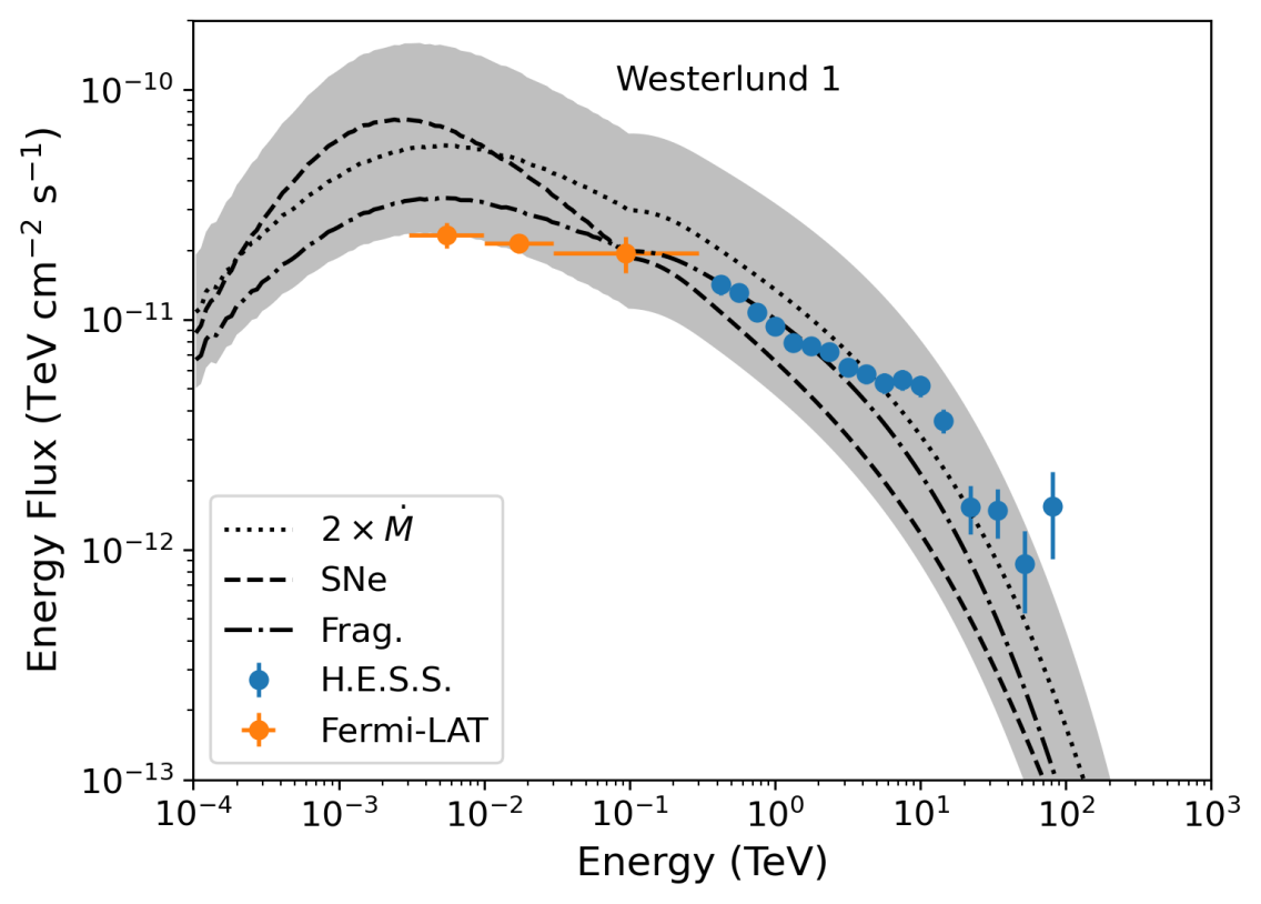
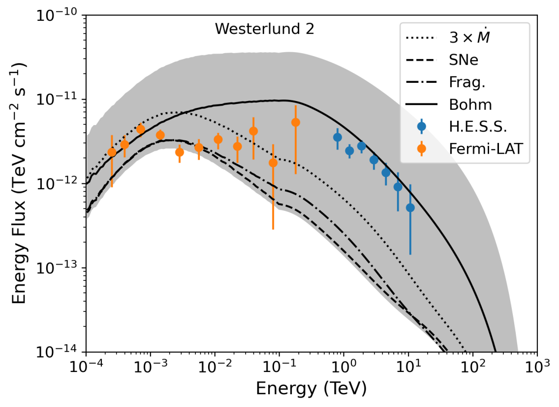
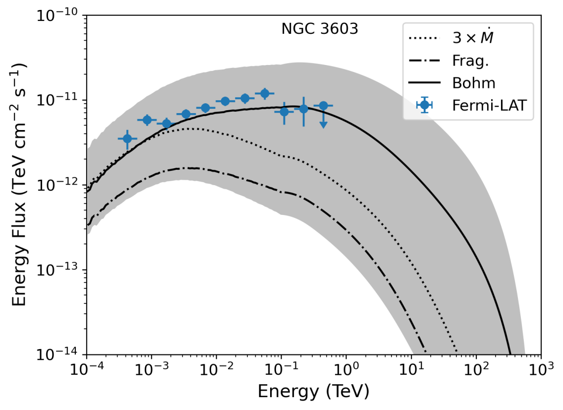
Figure 9: Comparison of measured $\gamma$-ray emission from three stellar clusters listed in the Gaia DR2 catalogue to predictions from this model. Shaded bands indicate reasonable model variations. Top: Wd1, data from (Ohm et al., 2013; Aharonian et al., 2022) Middle: Wd2, data from (Mestre et al., 2021; H.E.S.S. Collaboration et al., 2011) Bottom: NGC 3603, data from (Saha et al., 2020).

7 Comparison with $\gamma$-ray catalogues

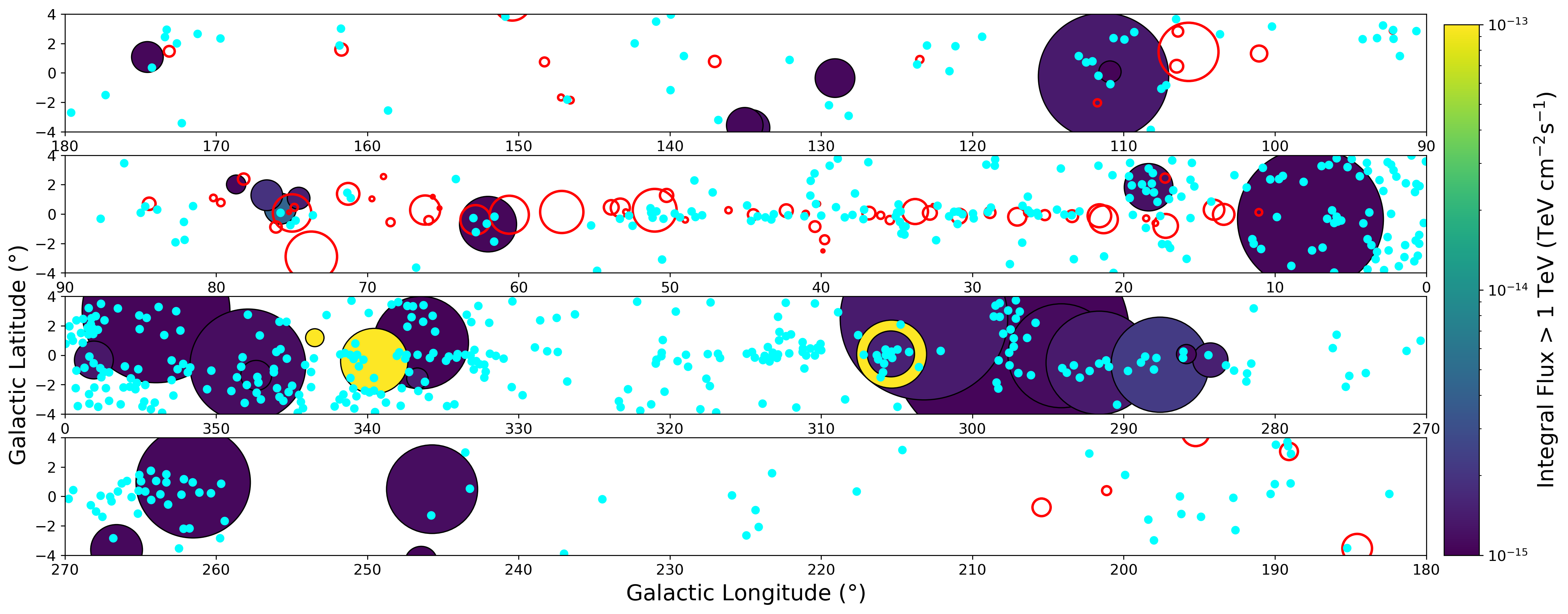
Figure 10: Predicted $\gamma$-ray flux from stellar cluster bubbles along the Galactic plane under the most optimistic scenario. Also indicated are sources from the first LHAASO catalogue (red circles) and unidentified sources from the 4FGL (cyan markers). The annular shape at $l\approx 305^{\circ}$ is a result of two overlapping clusters with different sizes.

We search for known $\gamma$-ray emitters in existing data from H.E.S.S., LHAASO, and Fermi-LAT as potential counterparts to the predicted emission from SC bubbles. Due to the limited expected fluxes for many of the systems in our sample, we constrain our discussion to the brightest objects listed in Table 2. The expected integral $\gamma$-ray flux above 1 TeV of these sources are shown in Figure 10, where we adopt the flux corresponding to the upper bound of our estimations, including contributions from SNRs, shell fragmentation and accounting for a potential underestimation of the cluster mass by a systematic factor 3 across the entire SC sample. The latter will lead to an increase in mass-loss rate and wind luminosity, thereby also increasing the size of the wind-blown bubble: because we are using maximal fluxes for Figure 10, the sizes adopted are also the largest reasonable angular sizes. For visual comparison of the spatial coincidences as described above, we indicate the locations of sources from the first LHAASO catalogue (1LHAASO) with red circles and of unidentified 4FGL point sources as cyan markers. The three brightest clusters, appearing yellow in Figure 10, correspond to the top three clusters listed in Table 2, namely Wd1, NGC 6231 and Danks 1.

7.1 Comparison to the H.E.S.S. catalogue

Within the H.E.S.S. Galactic Plane Survey (HGPS H. E. S. S. Collaboration et al., 2018), there are three sources which coincide with SCs listed in Table 2. These are HESS J1908+063 which coincides with Juchert 3; HESS J1646-458 with Wd1, and HESS J1023-575 with Wd2. The angular separation must lie within the region used for spectral extraction in the HGPS (RSpec) for the SC to be considered coincident with the $\gamma$-ray source. Wd1 and Wd2 are already the preferred associations for the aforementioned sources, where the $\gamma$-ray emission is indeed thought to be physically associated to the stellar cluster. For Wd1 the angular radius of the $\gamma$-ray emission $\sim 1^{\circ}$ is comparable to the predicted size of the wind-blown bubble, corresponding to a physical size of $\sim 230$ pc, whilst for Wd2 the physical size of $\sim 98$ pc corresponds to a predicted angular size of $\sim 1.5^{\circ}$ at the adopted distance of 4.47 kpc, much larger than the measured $\sim 0.3^{\circ}$ (Aharonian et al., 2022; H.E.S.S. Collaboration et al., 2011). Conversely, HESS J1908+063 is an unidentified $\gamma$-ray source with multiple possible counterparts: to date the source has been most often attributed to either the energetic pulsar PSR J1907+0602, the SNR G40.5-0.5 or a combination thereof (Li et al., 2021; Crestan et al., 2021). The coincidence of Juchert 3 with this source, an SC with the highest $\gamma$-ray fluxes predicted by our model among the baseline scenario, suggests another possible counterpart for this unidentified source.

7.2 Comparison to first LHAASO catalogue

The first LHAASO catalogue lists 43 sources of ultra-high-energy (UHE, $>$100 TeV) $\gamma$-ray emission, significantly increasing upon the 12 sources known as of 2021 Cao et al. (2024). As such, 1LHAASO is a suitable catalogue to cross-reference against the predictions of our model. The angular separation must be less than the 39% containment radius of the 2D Gaussian for the 1LHAASO morphology (R39) for the stellar cluster to be considered coincident with the $\gamma$-ray source. Although Wd1 and Wd2 are not visible to LHAASO, $\gamma$-ray emission coincident with Juchert 3 is also detected and given the identifier 1LHAASO J1908+0615u.

With an angular offset of $\sim 1.2^{\circ}$, NGC 6823 is nevertheless coincident with (within R39 of) 1LHAASO J1945+2424, an unidentified source also detected by HAWC as 2HWC J1949+244 (Abeysekara et al., 2017). No plausible accelerators have so far been suggested for this source, such that NGC 6823 provides a potential association for this unidentified source.

Although both Berkeley 87 and Dolidze 3 are coincident with the source 1LHAASO J2020+3638 within $\sim 1^{\circ}$, an association seems unlikely as the extent of the latter is $0.34^{\circ}$ and potentially associated with a known energetic pulsar in the vicinity.

7.3 Comparison to 4FGL catalogue

Sources from the 4FGL catalogue are here considered to be coincident with a SC if they lie within the bubble radius predicted by our baseline model. NGC 3603 is already provisionally associated with 4FGL J1115.1-6118 by Saha et al. (2020), which is the only 4FGL source coincident within $R_{s}$. Wd2 is also already associated with a 4FGL source, namely 4FGL J1023.3-5747e which is extended and best fit by a radial disk model (Abdollahi et al., 2020). Nevertheless, we find that there are at least two further unidentified 4FGL sources in within one bubble radius of Wd2 that hence could be associated.

For all other SCs listed in Table 2, we simply state the number of coincident unidentified 4FGL sources, i.e. within an angular separation $<R_{\rm b}$. Westerlund 1 – 5; NGC 6231 – 1; Danks 1 – 9; Berkeley 87 – 5; Trumpler 16 – 9; Danks 2 – 15; Markarian 50 – 12; Ruprecht 44 – 3; Hogg 15 – 1; UBC 344 – 4; Patchick 94 – 2; NGC 6611 – 11; NGC 6193 – 7; Juchert 3 – 3; Berkeley 59 – 7; NGC 1893 – 2; DC 5 – 3; NGC 6357 – 1; and UBC 558 – 3. Assuming that all unidentified 4FGL sources are evenly distributed in the Galactic plane, $|b|<5^{\circ}$, then at any position there should be on average one unidentified source within a radius of $\sim 1.2^{\circ}$. For most of the aforementioned clusters, the numbers are consistent with chance association, whilst for five clusters, there are at least a factor 4 times more coincident unidentified sources than would be expected by chance. These are Westerlund 1, Danks 1, UBC 344, NGC 6357 and UBC 558, for each of which further analysis is warranted to confirm or refute a potential association with the stellar cluster. For potential emission on angular scales $\gtrsim 1^{\circ}$, it is challenging to unambiguously associate potential sources without performing a dedicated analysis.

If, however, we apply a tighter restriction by evaluating coincidences occurring within the termination shock radius, then the following clusters (beyond Wd2 and NGC 3603) have plausible associations: Danks 1 with 4FGL J1312.3-6257 and 4FGL J1312.6-6231c, the latter of which is also coincident with Danks 2; Berkeley 87 with 4FGL J2022.6+3716c and Berkeley 59 with 4FGL J0002.1+6721c. A dedicated study for each of these SCs in turn would be required to conclusively establish an association with these as yet unidentified Fermi-LAT sources.

8 Conclusion and outlook

Massive SCs are promising candidate PeVatron accelerators, potentially responsible for CR acceleration up to the “knee” region. Young SCs ($\lesssim 3$ Myr), in particular, are expected to be powered by the collective wind from member stars, that may drive a termination shock at which particle acceleration can occur, with a large, wind-blown bubble expanding into the surrounding medium. Beyond $\sim 3$ Myr and up to $\sim 30$ Myr particle acceleration in a SC should be dominated, instead, by SNRs occurring inside of the bubble. Therefore, clusters younger than $\sim 30$ Myr are expected to behave as non-thermal particle emitters.

In this study, we apply the SC acceleration and transport model of Morlino et al. (2021) to known young and compact clusters catalogued by the Gaia satellite (Cantat-Gaudin et al., 2020), selecting 137 objects from its DR2. For these clusters, we first derived parameters needed for the wind model, namely wind velocities and mass-loss rates (see Celli et al., 2023), thus defining the system geometry (i.e. the expected location of the termination shock radius as well as of the wind-blown bubble radius) and the maximum particle energy achieved at the WTS. Additionally, we included the expected contribution from the SNe exploded within each cluster lifetime, in terms of both energetics and maximum energy achieved. Depending on the particle diffusion regime, we found that energies of $\gtrsim 1$ PeV are reached at the WTS in one (seven) SCs from Kraichnan (Bohm) diffusion, whilst the maximum energy reached at SNR shocks remains $\lesssim 500$ TeV in all cases.

We then predicted $\gamma$-ray and neutrino fluxes arising from hadronic collisions of the accelerated protons within the cluster bubble, thus evaluating which of the SCs among our sample could be detectable by CTA, LHAASO, and KM3NeT. Because the expected emission is integrated over the entire wind-blown bubble of typically large angular size, it appears necessary to take the degradation of experimental sensitivity due to extended source observations into account. As such, the number of systems for which emission from the bubble would be detectable drastically reduces to a few. Dedicated follow-up analyses accounting for the large angular size would be needed to either verify or refute the predictions made in this work. Accompanying data containing the results of this work, with flux predictions, is described in Table 5.

Among all SCs in our sample, three of them, namely Wd1, Wd2 and NGC 3603, have been already detected in $\gamma$-rays. We show that the reported spectra lie within the prediction of our model using a CR acceleration efficiency ranging between 5% and 10%. While the spectrum from Wd1 is in reasonable agreement with a Kraichnan diffusion model, Wd2 and NGC 3603 have a flatter spectrum below $\sim 1$ TeV, which suggests a diffusion regime in the bubble closer to the Bohm regime. We stress, however, that our conclusions for these three SCs should be taken as preliminary, as a more detailed analyses are required, where the sources morphology should be also taken into account. In particular, one should correctly evaluate the gas distribution in the bubble region. Moreover, if CRs are continuously produced by the cluster wind and injected into the surrounding ISM over $\sim$millions of years, then a characteristic $\propto 1/r$ CR density profile will emerge outside of the bubble (Aharonian et al., 2019).

Although the wind-blown bubbles around SCs are expected to yield comparatively low surface brightness $\gamma$-ray (and neutrino) emission, the expected flux could be locally enhanced by the presence of interstellar clouds. The availability of dense molecular material, causing increased hadronic interactions and subsequent emission on smaller angular scales, could indicate regions where the CR flux is higher than that of the Galactic CR sea, verifying that stellar clusters act as CR accelerators. The typically smaller angular size of interstellar clouds compared to that of cluster wind-blown bubbles may render such a search more easily feasible experimentally. This scenario will be considered in a forthcoming study complementing this work.

As a final comment we note that in this work we have only considered hadronic models, as the leptonic ones seem to be disfavoured, especially at the highest energies, if the magnetic field is amplified, as assumed in this work (see discussion in Menchiari et al., 2024, Sec. 5.3). However, we cannot rule out that inverse Compton scattering may be relevant for some of the SCs analysed here; additional work is required for a proper assessment of this issue.

Appendix A Stellar Cluster Physical Properties

	SC	GLON	GLAT	Age	Distance	$R_{\rm s}$	$R_{\rm b}$	$R_{\rm b}$	$E_{\rm max,Kol}^{\rm WTS}$	$E_{\rm max,Bohm}^{\rm WTS}$	$E_{\rm max}^{\rm SNe}$
		∘	∘	Myr	kpc	pc	pc	∘	PeV	PeV	PeV
1	Westerlund 1	339.546	-0.401	7.94	7.69	34.2	231.5	1.23	2.15	4.42	0.39
2	NGC 6231	343.476	1.190	13.80	1.48	22.7	206.5	1.46	0.42	1.40	0.26
3	Danks 1	305.342	0.074	1.00	1.87	10.4	55.6	1.16	0.54	3.06	0.51
4	Berkeley 87	75.756	0.361	8.32	1.64	13.8	127.8	2.84	0.25	0.93	0.25
5	Berkeley 86	76.650	1.276	10.96	1.62	14.7	141.7	0.51	0.23	0.76	0.23
6	Trumpler 16	287.599	-0.646	13.49	2.11	16.0	162.4	3.88	0.22	0.79	0.22
7	Danks 2	305.390	0.089	2.00	2.23	10.9	72.6	3.04	0.40	2.14	0.40
8	Dolidze 3	74.545	1.072	8.91	2.09	13.9	126.2	1.12	0.24	0.76	0.24
9	Westerlund 2	284.272	-0.328	3.98	4.47	12.6	97.8	1.49	0.33	1.52	0.33
10	NGC 3603	291.624	-0.518	1.00	7.16	9.9	53.9	0.42	0.50	2.83	0.50
11	Markarian 50	111.335	-0.239	11.48	3.20	15.0	148.5	3.91	0.23	0.82	0.23
12	Ruprecht 44	245.722	0.492	14.45	5.75	16.4	168.6	4.36	0.22	0.78	0.22
13	Hogg 15	302.048	-0.242	2.19	3.02	8.0	58.6	0.86	0.33	1.03	0.33
14	Sher 1	289.635	-0.242	13.18	6.07	15.8	160.3	0.57	0.22	0.80	0.22
15	UBC 344	18.354	1.820	3.47	1.92	7.3	65.3	1.10	0.27	0.69	0.27
16	Patchick 94	336.458	0.855	3.55	3.18	7.2	65.4	1.10	0.26	0.67	0.26
17	NGC 6611	16.962	0.811	2.14	1.65	4.5	40.4	2.20	0.25	0.43	0.25
18	NGC 6193	336.694	-1.576	5.13	1.26	5.1	57.4	1.68	0.19	0.27	0.19
19	Juchert 3	40.354	-0.701	1.00	1.48	3.9	28.3	1.49	0.32	0.55	0.32
20	Berkeley 59	118.230	5.019	1.26	1.00	3.2	26.5	2.98	0.26	0.33	0.26
21	NGC 6823	59.423	-0.139	2.40	2.33	4.2	39.6	0.25	0.23	0.34	0.23
22	NGC 1893	173.577	-1.634	4.37	3.22	4.8	53.1	2.84	0.20	0.29	0.20
23	DC 5	286.795	-0.502	1.12	4.43	3.7	28.6	1.21	0.30	0.48	0.30
24	NGC 6357	353.166	0.890	1.00	1.77	3.0	23.6	0.24	0.28	0.34	0.28
25	UBC 558	347.350	-1.375	7.24	2.83	4.8	60.8	0.96	0.16	0.18	0.16

Table 2: Properties of the stellar clusters with the brightest predicted gamma-ray emission, ranked according to integral flux above 1 TeV over the wind-blown bubble.

Appendix B Stellar Cluster Flux Predictions

	SC	$F_{\gamma}$ ($>$1 TeV)	$F_{\gamma}^{\rm ul}$ ($>$1 TeV)	$F_{\gamma}$ ($>$10 TeV)	$F_{\gamma}^{\rm ul}$ ($>$10 TeV)	$F_{\gamma}$ (7 TeV)	$F_{\gamma}^{\rm ul}$ (7 TeV)	$F_{\nu_{\mu}}$ ($>$ 10 TeV)
1	Westerlund 1	6.3e-12	4.4e-12	6.4e-13	4.1e-11	2.5e-14	–	1.1e-13
2	NGC 6231	4.7e-12	2.9e-12	1.5e-13	2.7e-11	1.2e-14	–	1.8e-14
3	Danks 1	2.3e-12	1.3e-12	9.8e-14	1.2e-11	6.5e-15	–	1.2e-14
4	Berkeley 87	3.6e-13	–	5e-15	–	5.8e-16	1.4e-13	4e-16
5	Berkeley 86	2.4e-13	–	2.5e-15	–	3.4e-16	1.2e-13	1.8e-16
6	Trumpler 16	2e-13	2.2e-12	2.6e-15	2.1e-11	3.1e-16	–	2e-16
7	Danks 2	1.6e-13	1.2e-12	5.1e-15	1.1e-11	3.9e-16	–	5.7e-16
8	Dolidze 3	1.5e-13	–	1.4e-15	–	2e-16	1.3e-13	9.1e-17
9	Westerlund 2	1.4e-13	1.6e-11	3.3e-15	1.5e-10	2.9e-16	–	3.4e-16
10	NGC 3603	1.3e-13	8.3e-13	5e-15	7.8e-12	3.5e-16	–	5.9e-16
11	Markarian 50	1.2e-13	–	1.5e-15	–	1.8e-16	7.7e-15	1.1e-16
12	Ruprecht 44	5.1e-14	–	6.5e-16	–	7.9e-17	3.3e-14	5.1e-17
13	Hogg 15	2.5e-14	3.2e-12	2e-16	3e-11	3.2e-17	–	1.3e-17
14	Sher 1	2.2e-14	9.5e-13	2.8e-16	8.8e-12	3.4e-17	–	2.2e-17
15	UBC 344	1.8e-14	2.3e-12	6.4e-17	2.2e-11	1.7e-17	1.7e-13	3.1e-18
16	Patchick 94	5.9e-15	5.8e-12	1.9e-17	5.4e-11	5.3e-18	–	9.1e-19
17	NGC 6611	9.4e-16	2.4e-12	1.8e-19	2.2e-11	1.8e-19	3.4e-13	5e-21
18	NGC 6193	6.5e-16	1.6e-12	2.2e-20	1.5e-11	4.1e-20	–	4.7e-22
19	Juchert 3	3.7e-16	8.3e-12	1.1e-19	7.7e-11	8.8e-20	2.4e-13	3.2e-21
20	Berkeley 59	2.2e-16	–	1.9e-21	–	5.7e-21	2.9e-14	3.4e-23
21	NGC 6823	2.1e-16	8.9e-13	1e-20	8.3e-12	1.7e-20	5.8e-14	2.3e-22
22	NGC 1893	1.1e-16	–	4.4e-21	–	7.7e-21	2.3e-15	9.7e-23
23	DC 5	9.4e-17	3.6e-12	1.3e-20	3.3e-11	1.4e-20	–	3.4e-22
24	NGC 6357	7.8e-17	1.3e-12	6.6e-22	1.2e-11	2e-21	–	1.2e-23
25	UBC 558	2e-17	1.3e-12	3.6e-23	1.2e-11	1.9e-22	–	5.5e-25

Table 3: Properties of the stellar clusters with the brightest predicted emission in ranked order. Integral flux values are given in units of TeV cm^-2 s^-1 and differential flux values in units of TeV^-1 cm^-2 s^-1. Upper limits from the HGPS (corresponding to the angular size of the bubble or $0.6^{\circ}$, whichever is smaller) and 3HWC (corresponding to the nearest available angular size) are provided where available (H. E. S. S. Collaboration et al. 2018; Albert et al. 2020).

	SC	$F_{\gamma}$ ($>$1 TeV)	$F_{\gamma}^{\rm ul}$ ($>$1 TeV)	$F_{\gamma}$ ($>$10 TeV)	$F_{\gamma}^{\rm ul}$ ($>$10 TeV)	$F_{\gamma}$ (7 TeV)	$F_{\gamma}^{\rm ul}$ (7 TeV)	$F_{\nu_{\mu}}$ ($>$ 10 TeV)
1	NGC 6231	1.1e-10	2.9e-12	7.4e-12	2.7e-11	3.8e-13	–	1e-12
2	Westerlund 1	9e-11	4.4e-12	1.5e-11	4.1e-11	4.1e-13	–	2.8e-12
3	Danks 1	3.6e-11	1.3e-12	3.1e-12	1.2e-11	1.4e-13	–	4.7e-13
4	Berkeley 87	1.2e-11	–	5.3e-13	–	3.3e-14	1.4e-13	7e-14
5	Trumpler 16	6.8e-12	2.2e-12	2.7e-13	2.1e-11	1.8e-14	–	3.4e-14
6	Berkeley 86	6.5e-12	–	1.8e-13	–	1.5e-14	1.2e-13	1.9e-14
7	Dolidze 3	4.1e-12	–	1e-13	–	9.3e-15	1.3e-13	1.1e-14
8	Markarian 50	3.1e-12	–	9.8e-14	–	7.7e-15	7.7e-15	1.1e-14
9	Westerlund 2	3e-12	1.6e-11	1.7e-13	1.5e-10	9.6e-15	–	2.3e-14
10	Danks 2	2.9e-12	1.2e-12	2e-13	1.1e-11	1e-14	–	2.8e-14
11	UBC 334	2.8e-12	1.6e-12	6.9e-14	1.5e-11	7.2e-15	–	5.8e-15
12	NGC 4755	2.5e-12	2.6e-11	1.1e-13	2.4e-10	8e-15	–	1.2e-14
13	NGC 869	2.1e-12	–	7.8e-14	–	6.4e-15	5.3e-15	7.7e-15
14	NGC 6193	2.1e-12	1.6e-12	1.8e-13	1.5e-11	8.7e-15	–	2.5e-14
15	NGC 3603	2.1e-12	2.4e-12	1.7e-13	2.3e-11	7.8e-15	–	2.4e-14
16	NGC 1502	1.9e-12	–	7.6e-14	–	6e-15	2.5e-14	7.7e-15
17	NGC 3766	1.7e-12	1.2e-12	3.6e-14	1.1e-11	4.1e-15	–	2.9e-15
18	UBC 344	1.6e-12	2.3e-12	1.3e-13	2.2e-11	5.4e-15	1.7e-13	2.1e-14
19	Ruprecht 44	1.6e-12	–	6e-14	–	4.2e-15	3.3e-14	7.2e-15
20	IC 2395	1.5e-12	3e-12	2.1e-14	2.8e-11	3e-15	–	1.5e-15
21	NGC 1960	1.4e-12	–	1.6e-14	–	2.6e-15	1.4e-14	1.1e-15
22	NGC 6318	1.2e-12	9.5e-12	6.2e-14	8.8e-11	4.2e-15	–	7e-15
23	Collinder 197	1.2e-12	2.9e-12	2.9e-14	2.7e-11	3e-15	–	2.4e-15
24	NGC 884	1.2e-12	–	3.3e-14	–	3.2e-15	6e-15	2.9e-15
25	NGC 6910	1e-12	–	3.3e-14	–	3e-15	1.3e-13	3.1e-15

Table 4: Same as for table 3, except providing the flux values for the maximal scenario. Note that the upper limits take changes in the bubble radius into account.

Appendix C Description of online data

Column	Data type	Unit	Description
cluster	str17		Unified cluster name
d	float64	kpc	Distance to the cluster
Rs	float64	pc	Cluster shock radius
Rb	float64	pc	Cluster bubble physical radius
Rb	float64	deg	Cluster bubble angular radius
EF1	float64	$\rm{TeV}$ / ($\rm{cm}^{2}$ s)	Integrated gamma-ray energy flux from the cluster bubble above 1 TeV
EF10	float64	$\rm{TeV}$ / ($\rm{cm}^{2}$ s)	Integrated gamma-ray energy flux from the cluster bubble above 10 TeV
EFnu10	float64	$\rm{TeV}$ / ($\rm{cm}^{2}$ s)	Integrated muon neutrino energy flux from the cluster bubble above 10 TeV
Emax	float64	PeV	Maximum particle energy

Table 5: Information on columns provided in the fits data product. This file is provided for both the baseline and the maximal scenarios.

References

- Abdollahi et al. (2020) Abdollahi, S., Acero, F., Ackermann, M., et al. 2020, ApJS, 247, 33
- Abeysekara et al. (2017) Abeysekara, A. U., Albert, A., Alfaro, R., et al. 2017, ApJ, 843, 40
- Abeysekara et al. (2020) Abeysekara, A. U., Albert, A., Alfaro, R., et al. 2020, Phys. Rev. Lett., 124, 021102
- Aguilar et al. (2015) Aguilar, M., Aisa, D., Alpat, B., et al. 2015, Phys. Rev. Lett., 114, 171103
- Aharonian et al. (2022) Aharonian, F., Ashkar, H., Backes, M., et al. 2022, A&A, 666, A124
- Aharonian et al. (2019) Aharonian, F., Yang, R., & de Oña Wilhelmi, E. 2019, Nature Astronomy, 3, 561
- Albert et al. (2020) Albert, A., Alfaro, R., Alvarez, C., et al. 2020, ApJ, 905, 76
- Ambrogi et al. (2018) Ambrogi, L., Celli, S., & Aharonian, F. 2018, Astroparticle Physics, 100, 69
- Bell et al. (2013) Bell, A. R., Schure, K. M., Reville, B., & Giacinti, G. 2013, MNRAS, 431, 415
- Blasi (2013) Blasi, P. 2013, A&A Rev., 21, 70
- Blasi & Morlino (2023) Blasi, P. & Morlino, G. 2023, MNRAS, 523, 4015
- Cantat-Gaudin et al. (2020) Cantat-Gaudin, T., Anders, F., Castro-Ginard, A., et al. 2020, A&A, 640, A1
- Cao et al. (2024) Cao, Z., Aharonian, F., An, Q., et al. 2024, The Astrophysical Journal Supplement Series, 271, 25
- Cao et al. (2021) Cao, Z., Aharonian, F. A., An, Q., et al. 2021, Nature, 594, 33
- Celli et al. (2020) Celli, S., Aharonian, F., & Gabici, S. 2020, ApJ, 903, 61
- Celli & Peron (2024) Celli, S. & Peron, G. 2024, arXiv e-prints, arXiv:2403.03731
- Celli et al. (2023) Celli, S., Specovius, A., Menchiari, S., Mitchell, A., & Morlino, G. 2023, arXiv e-prints, arXiv:2311.09089
- Cherenkov Telescope Array Observatory & Cherenkov Telescope Array Consortium (2021) Cherenkov Telescope Array Observatory & Cherenkov Telescope Array Consortium. 2021, CTAO Instrument Response Functions - prod5 version v0.1
- Crestan et al. (2021) Crestan, S., Giuliani, A., Mereghetti, S., et al. 2021, MNRAS, 505, 2309
- Dwarkadas (2005) Dwarkadas, V. V. 2005, ApJ, 630, 892
- Dwarkadas (2007) Dwarkadas, V. V. 2007, ApJ, 667, 226
- Gaia Collaboration (2018) Gaia Collaboration. 2018, A&A, 616, A1
- Gennaro et al. (2011) Gennaro, M., Brandner, W., Stolte, A., & Henning, T. 2011, MNRAS, 412, 2469
- Gupta et al. (2020) Gupta, S., Nath, B. B., Sharma, P., & Eichler, D. 2020, MNRAS, 493, 3159
- Härer et al. (2023) Härer, L. K., Reville, B., Hinton, J., Mohrmann, L., & Vieu, T. 2023, A&A, 671, A4
- H. E. S. S. Collaboration et al. (2018) H. E. S. S. Collaboration, Abdalla, H., Abramowski, A., et al. 2018, A&A, 612, A1
- H.E.S.S. Collaboration et al. (2011) H.E.S.S. Collaboration, Abramowski, A., Acero, F., et al. 2011, A&A, 525, A46
- Hunt & Reffert (2023) Hunt, E. L. & Reffert, S. 2023, A&A, 673, A114
- Kelner et al. (2006) Kelner, S. R., Aharonian, F. A., & Bugayov, V. V. 2006, Phys. Rev. D, 74, 034018
- Lancaster et al. (2021a) Lancaster, L., Ostriker, E. C., Kim, J.-G., & Kim, C.-G. 2021a, ApJ, 914, 89
- Lancaster et al. (2021b) Lancaster, L., Ostriker, E. C., Kim, J.-G., & Kim, C.-G. 2021b, ApJ, 914, 90
- Lhaaso Collaboration (2024) Lhaaso Collaboration. 2024, Science Bulletin, 69, 449
- Li et al. (2021) Li, J., Liu, R.-Y., de Oña Wilhelmi, E., et al. 2021, ApJ, 913, L33
- Menchiari (2023) Menchiari, S. 2023, Probing star clusters as cosmic ray factories
- Menchiari et al. (2024) Menchiari, S., Morlino, G., Amato, E., Bucciantini, N., & Beltrán, M. T. 2024, arXiv e-prints, arXiv:2402.07784
- Mestre et al. (2021) Mestre, E., de Oña Wilhelmi, E., Torres, D. F., et al. 2021, MNRAS, 505, 2731
- Morlino et al. (2021) Morlino, G., Blasi, P., Peretti, E., & Cristofari, P. 2021, MNRAS, 504, 6096
- Navarete et al. (2022) Navarete, F., Damineli, A., Ramirez, A. E., Rocha, D. F., & Almeida, L. A. 2022, MNRAS, 516, 1289
- Ohm et al. (2013) Ohm, S., Hinton, J. A., & White, R. 2013, MNRAS, 434, 2289
- Rocha et al. (2022) Rocha, D. F., Almeida, L. A., Damineli, A., et al. 2022, MNRAS, 517, 3749
- Rosslowe & Crowther (2015) Rosslowe, C. K. & Crowther, P. A. 2015, MNRAS, 447, 2322
- Saha et al. (2020) Saha, L., Domínguez, A., Tibaldo, L., et al. 2020, ApJ, 897, 131
- Unbehaun et al. (2024) Unbehaun, T., Mohrmann, L., Funk, S., et al. 2024, European Physical Journal C, 84, 112
- van Eeden (2024) van Eeden, T. 2024, arXiv e-prints, arXiv:2402.08363
- Vieu et al. (2020) Vieu, T., Gabici, S., & Tatischeff, V. 2020, MNRAS, 494, 3166
- Vieu & Reville (2023) Vieu, T. & Reville, B. 2023, MNRAS, 519, 136
- Vieu et al. (2022) Vieu, T., Reville, B., & Aharonian, F. 2022, MNRAS, 515, 2256
- Weaver et al. (1977) Weaver, R., McCray, R., Castor, J., Shapiro, P., & Moore, R. 1977, ApJ, 218, 377
- Weidner & Kroupa (2004) Weidner, C. & Kroupa, P. 2004, MNRAS, 348, 187
- Yang & Aharonian (2017) Yang, R.-z. & Aharonian, F. 2017, A&A, 600, A107