Effect of Coriolis Force on Electrical Conductivity Tensor for Rotating Hadron Resonance Gas

Abstract

We have investigated the influence of the Coriolis force on the electrical conductivity of hadronic matter formed in relativistic nuclear collisions, employing the Hadron Resonance Gas (HRG) model. A rotating matter in the peripheral heavy ion collisions can be expected from the initial stage of quark matter to late-stage hadronic matter. Present work is focused on rotating hadronic matter, whose medium constituents - hadron resonances can face a non-zero Coriolis force, which can influence the hadronic flow or conductivity. We estimate this conductivity tensor by using the relativistic Boltzmann transport equation. In the absence of Coriolis force, an isotropic conductivity tensor for hadronic matter is expected. However, our study finds that the presence of Coriolis force can generate an anisotropic conductivity tensor with three main conductivity components - parallel, perpendicular, and Hall, similar to the effect of Lorentz force at a finite magnetic field. Our study has indicated that a noticeable anisotropy of conductivity tensor can be found within the phenomenological range of angular velocity $\Omega=0.001-0.02$ GeV and hadronic scattering radius $a=0.2-2$ fm.

I Introduction

In off-central heavy ion collision (HIC) experiments, a large orbital angular momentum (OAM) can be produced, and this initial OAM depends upon factors such as system size, collision geometry, and collision energy, ranging from $10^{3}\hbar$ to $10^{7}\hbar$ [1, 2, 3]. After the collision, the spectators carry some of the angular momenta, and the rest is transferred to the produced quark-gluon matter. The initial OAM transferred to the medium is stored in the initial fluid velocity profile of the quark matter and at a later stage in the hadronic matter in the form of local vorticity. This OAM can induce various effects within the medium, like spin polarization, chiral vortical effect (CVE), etc. The vorticity leads to the alignment of hadrons along its direction, influenced by spin-orbit coupling. When considering all space-time points on the freeze-out hypersurface, local polarization accumulates, resulting in a global polarization aligned with the reaction plane or the angular momentum of the colliding nuclei. The global polarization of $\Lambda$ and $\bar{\Lambda}$ particles has been measured by the STAR Collaboration in Au+Au collisions across a range of collision energies ($\sqrt{s_{NN}}=$7.7-200 GeV), revealing a decreasing trend with collision energies [1]. Moreover, in the recent study with improved statistics at $\sqrt{s_{NN}}=$ 200 GeV, a polarization dependence on the event-by-event charge asymmetry was observed, indicating a potential contribution to the global polarization from the axial current induced by the initial magnetic field [4]. Additionally, spin alignment has also been observed in vector mesons, with recent measurements conducted at RHIC and LHC further contributing to our understanding of spin phenomena in heavy ion collisions [5, 6, 7].

Now, from the theoretical direction, the effect of large OAM on the medium constituents has been studied even before the experimental work of STAR Collaboration [1] in the Refs. [2, 3, 8, 9, 10, 11, 12, 13, 14]. The experimental finding of global polarization of $\Lambda$ and $\bar{\Lambda}$ particles in $2017$  [1] also stimulated many theoretical investigations of vorticity and spin polarization effects in HIC [15, 16, 17, 18, 19, 20, 21, 22, 23, 24, 25]. The study vorticity and the polarization of the particles produced by HICs has been done by multitude of theoretical approaches. The references [26, 27, 28, 29, 30, 31, 32, 33, 34, 35, 36, 37, 38, 39, 40, 41, 42], with the help of covariant Wigner functions and quantum kinetic equations, have described the chiral effects and the spin polarization of final state particles. On the other hand, the authors of Refs. [43, 3, 8, 44, 9, 10, 45, 15] used the theory of relativistic statistical mechanics for a plasma in global equilibrium under rotation to describe the polarization of particles emitted from the kinetic freeze-out hypersurface. In contrast, in Refs. [11, 2, 12, 13, 46, 14], the spin-orbit interaction in QCD has been used to describe the transfer of initial OAM density into the spin angular momentum, ultimately resulting in the spin polarization of particles. Moreover, the authors of Refs. [47, 17, 18, 48, 49, 50, 19, 51, 52, 53, 54] have developed a kinetic framework to establish the equations of spin hydrodynamics by including the spin tensor. In addition, several transport and hydrodynamical models  [55, 56, 57, 58, 16, 20, 59, 21, 22, 23, 24, 25] have also been used to estimate spin polarization and vorticity results in HIC quantitatively. Thermodynamics of the hadronic medium under rotation have recently been explored by Refs. [60, 61, 62]. The phase structure of rigidly rotating plasma has been explored in Refs. [63, 64]. The Lattice Quantum Chromodynamics (LQCD) calculations in the presence of rotations can be found in the Refs. [65, 66].

There is a similarity between magnetic field and rotation. The picture of Lorentz force in the presence of magnetic fields is quite similar to the picture of the Coriolis force in presence of rotation. In Refs. [67, 68, 69], the equivalence between the Coriolis force and Lorentz force has been explored. In the presence of magnetic fields, the transport coefficients of the systems become an-isotropic[70, 71, 72, 73, 74, 75, 76, 77, 78, 79, 70, 80, 81, 82, 83]. Accordingly, one should expect the anisotropic structure of the transport coefficients in a rotating frame due to the effect of the Coriolis force. In this paper, we will show how the electrical conductivity of the rotating hadronic matter formed in HIC can be modified in the presence of Coriolis force. In the papers  [84, 85], the authors have described how a rotating medium’s shear viscosity and electrical conductivity become anisotropic in the presence of Coriolis force. Here, we have extended the formalism of Ref. [85] from non-relativistic to the relativistic case, which is applicable to calculate the electrical conductivity of the rotating hadronic matter. To fulfill this purpose, we employed the relativistic Boltzmann transport equation in relaxation time approximation with the inclusion of Coriolis force. We modeled our rotating hadronic medium by resorting to the popular HRG model. This model is founded upon principles derived from statistical mechanics of multi-hadron species. Using S-matrix calculation, it has been shown that in the presence of narrow resonances, the thermodynamics of the interacting gas of hadrons can be approximated by the ideal gas of hadrons and its resonances [86, 87]. The HRG model has been extensively used to study thermodynamics [88, 89] and conserved charge fluctuations [90, 91, 92, 93, 94], as well as transport coefficients [95, 96, 97, 98, 99, 100, 101, 102, 103, 104, 105], which are quite accepted for heavy ion collision phenomenology. Recently, Refs. [71, 72, 78, 79] have demonstrated the role of Lorentz force in creating anisotropic transportation of HRG system. However, the role of Coriolis force in creating similar kind of anisotropic transportation for HRG system has not been studied yet and here, we are first time going for this kind of investigation.

The article is arranged as follows: in Sec. II, we develop the necessary formalism needed for calculating electrical conductivity tensor in the presence of rotation. The master formula for hadronic matter with the hadron resonance gas model (HRG) and QGP with massless approximation is provided in II.1 and Sec. II.2 from which the results are generated. In Sec. III, we present the numerical results with the plots of the variation of conductivity for QGP and hadronic matter both in the presence and absence of rotation. The article is summarised in Sec. IV.

II Formalism

Let us consider a rotating system of hadrons moving with the velocities $\vec{v}_{r}=\frac{\vec{p}_{r}}{E_{r}}$. The micro- and macro-scopic expressions of current density for these collections of hadron resonances under an applied electric field $\vec{\tilde{E}}\equiv\tilde{E}\hat{e}$ are,

$$J^{i} = \sum\limits_{r}J_{r}^{i}=\sum\limits_{r}g_{r}q_{r}\int{\frac{d^{3}\vec{p_{r}}}{{(2\pi})^{3}}}\frac{p^{i}_{r}}{E_{r}}\delta{f_{r}},$$ (1)

$$J^{i} = \sum\limits_{r}J_{r}^{i}=\sum\limits_{r}\sigma_{r}^{ij}\tilde{E}_{j}\equiv\sigma^{ij}\tilde{E}_{j},$$ (2)

where $r$ is the label characterizing the different hadrons and resonances with charge $q_{r}$ and degeneracy $g_{r}$. The $\delta{f_{r}}$ quantifies the deviation of the system from local equilibrium. $J^{i}=\sum\limits_{r}J_{r}^{i}$ and $\sigma^{ij}=\sum\limits_{r}\sigma_{r}^{ij}$ are respectively the current density and conductivity tensor due to all the hadronic species comprised of baryons and mesons. The microscopic expression of current density in the HRG phase provided in Eq. (1) can be compared with the macroscopic expression $J^{i}=\sigma^{ij}\tilde{E}_{j}$ to obtain the conductivity tensor $\sigma^{ij}$. The deviation function $\delta f_{r}$ written in Eq. (1) corresponds to the difference between the total distribution function and equilibrium distribution function for the $r$th hadronic species, i.e., $\delta f_{r}=f_{r}-f_{r}^{0}$. We will assume that the system is slightly out of equilibrium so that $\delta f_{r}$ can be treated as a perturbation. The perturbation $\delta f_{r}$ can be determined by using the Boltzmann transport equation (BTE). We have a hadronic medium rotating with an angular velocity $\vec{\Omega}\equiv\Omega\hat{\omega}$. The $r^{\rm th}$ hadron of the medium have a random part of the velocity $\vec{v}_{r}$ on top of the overall angular part of the velocity $\vec{\Omega}\times\vec{r}$, where $\vec{r}$ denotes the position of hadron. Each hadron of the rotating HRG will feel the Coriolis force, whose magnitude is given by $2m\gamma_{v}(\vec{v}_{r}\times\vec{\Omega})$ [106], where $\gamma_{v}=1/\sqrt{1-v_{r}^{2}}$. The BTE for the rotating HRG, incorporating the Coriolis force within the relaxation time approximation (RTA), is given by,

$$[q\vec{\tilde{E}}+2m\gamma_{v}(\vec{v}\times\vec{\Omega})]\cdot\frac{\partial}{\partial\vec{p}}(f^{0}+\delta f)=-\frac{\delta f}{\tau_{c}},$$ (3)

where we have suppressed the index $r$ in writing Eq. (3), which will be retained during the calculation of total conductivity. The local equilibrium distribution function is,

$$f^{0}=1/\exp\Big(\frac{p^{\nu}u_{\nu}-\mu(\vec{r},t)}{T(\vec{r},t)}\Big{missing})-a,$$

where $u_{\nu}=(\gamma_{u},-\gamma_{u}\vec{u})$ is the fluid-four velocity and $p^{\nu}=(E,\vec{p})$ is four-momentum for the hadrons and resonances. $a=-1$ for baryons and $a=+1$ for mesons. Substituting the local equilibrium distribution function $f^{0}$ in Eq. 3, we have,

$$q\vec{\tilde{E}}\cdot\frac{\partial f^{0}}{\partial\vec{p}}+2m\gamma_{v}(\vec{v}\times\vec{\Omega})\cdot\frac{\partial f^{0}}{\partial\vec{p}}+2m\gamma_{v}(\vec{v}\times\vec{\Omega})\cdot\frac{\partial\delta f}{\partial\vec{p}}=-\frac{\delta f}{\tau_{c}}$$

$$\implies q\vec{\tilde{E}}\cdot\frac{\partial f^{0}}{\partial E}\vec{v}+2m\gamma_{v}(\vec{v}\times\vec{\Omega})\cdot\frac{\partial f^{0}}{\partial E}\vec{v}+2m\gamma_{v}(\vec{v}\times\vec{\Omega})\cdot\frac{\partial\delta f}{\partial\vec{p}}=-\frac{\delta f}{\tau_{c}}$$

$$\implies\frac{\partial f^{0}}{\partial E}\vec{v}\cdot(q\vec{\tilde{E}})+2m\gamma_{v}(\vec{v}\times\vec{\Omega})\cdot\frac{\partial\delta f}{\partial\vec{p}}=-\frac{\delta f}{\tau_{c}},$$ (4)

where we have used the result $\frac{\partial f^{0}}{\partial\vec{p}}=\frac{\partial f^{0}}{\partial E}\vec{v}$, which holds in static limit $\vec{u}=0$.

One has to solve Eq. 4 for $\delta f$ to determine HRG current density $J^{i}$ from Eq. 1. Let us make an educated guess of the form: $\delta f=-\vec{p}\cdot\vec{X}\big{(}\frac{\partial f^{0}}{\partial E}\big{)}$, where we have to find out $\vec{X}$. Our system of rotating HRG is no longer isotropic because of the presence of the angular velocity vector $\vec{\Omega}=\Omega\hat{\omega}$. We have two unit vectors $\hat{\omega}$ and $\hat{e}$ in our hand, which can be used to construct another unit vector $\hat{e}\times\hat{\omega}$ perpendicular to both $\hat{\omega}$ and $\hat{e}$. In general, the current density in rotating HRG can have components along $\hat{\omega}$, $\hat{e}$, and $\hat{e}\times\hat{\omega}$. Since the vector $\vec{X}$ determines the form of the current density through Eq. 1, we can guess the following decomposition of $\vec{X}=\alpha\hat{e}+\beta\hat{\omega}+\gamma(\hat{e}\times\hat{\omega})$ with the unknowns $\alpha$, $\beta$, and $\gamma$. These unknowns would be determined by substituting $\delta f$ in the Eq. (4) and can be re-written as,

$$\frac{\partial f^{0}}{\partial E}\vec{v}\cdot(q\vec{\tilde{E}})+2\vec{p}\cdot\left[\vec{\Omega}\times\frac{\partial\delta f}{\partial\vec{p}}\right] =\frac{-\delta f}{\tau_{c}}$$

$$\implies\frac{\partial f^{0}}{\partial E}\frac{\vec{p}}{E}\cdot(q\vec{\tilde{E}})+2\vec{p}\cdot\left[\vec{\Omega}\times\frac{\partial(-\vec{p}\cdot\vec{X}\frac{\partial f^{0}}{\partial E})}{\partial\vec{p}}\right] =\frac{\vec{p}\cdot\vec{X}}{\tau_{c}}\frac{\partial f^{0}}{\partial E},$$

which, after simplification, becomes,

$$\left[\frac{q\tilde{\vec{E}}}{E}+2(\vec{X}\times\vec{\Omega})\right]\cdot\vec{p}\frac{\partial f^{0}}{\partial E}=\frac{\vec{X}}{\tau_{c}}\cdot\left(\vec{p}\frac{\partial f^{0}}{\partial E}\right),$$ (5)

since $\vec{p}$ is arbitrary in Eq. 5, the following relation valid for $\vec{X}$,

$$\left[\frac{q\tilde{\vec{E}}}{E}+2(\vec{X}\times\vec{\Omega})\right]=\frac{\vec{X}}{\tau_{c}}~{}.$$ (6)

Substituting the result, $\vec{X}\times\vec{\Omega}=-\gamma\Omega\hat{e}+\gamma\Omega(\hat{\omega}\cdot\hat{e})\hat{\omega}+\alpha\Omega(\hat{e}\times\hat{\omega})$, in Eq. 6, we have,

$$\Big{(}\frac{q\vec{\tilde{E}}}{E}-2\Omega\gamma\Big{)}\hat{e}+2\gamma\Omega(\hat{\omega}\cdot\hat{e})\hat{\omega}+2\alpha\Omega(\hat{e}\times\hat{\omega})=\frac{\alpha}{\tau_{c}}\hat{e}+\frac{\beta}{\tau_{c}}\hat{\omega}+\frac{\gamma}{\tau_{c}}(\hat{e}\times\hat{\omega})~{}.$$ (7)

By equating the coefficients of the linearly independent basis vectors in Eq. 7, we get,

$$\frac{q\tilde{E}}{E}-\frac{\gamma}{\tau_{\Omega}} =\frac{\alpha}{\tau_{c}}, \frac{\gamma}{\tau_{\Omega}}(\hat{\omega}.\hat{e}) =\frac{\beta}{\tau_{c}}, \frac{\alpha}{\tau_{\Omega}} =\frac{\gamma}{\tau_{c}},$$

where $\tau_{\Omega}\equiv\frac{1}{2\Omega}$. Simplifying the above three equations, we get the following values for $\alpha,\beta,\text{ and }\gamma$

$$\alpha =\frac{\tau_{c}\big{(}\frac{q\tilde{E}}{E}\big{)}}{1+\big{(}\frac{\tau_{c}}{\tau_{\Omega}}\big{)}^{2}}, \gamma =\frac{\tau_{c}\big{(}\frac{\tau_{c}}{\tau_{\Omega}}\big{)}\big{(}\frac{q\tilde{E}}{E}\big{)}}{1+\big{(}\frac{\tau_{c}}{\tau_{\Omega}}\big{)}^{2}}, \beta =\frac{\tau_{c}\big{(}\frac{\tau_{c}}{\tau_{\Omega}}\big{)}^{2}(\hat{\omega}.\hat{e})\big{(}\frac{q\tilde{E}}{E}\big{)}}{1+\big{(}\frac{\tau_{c}}{\tau_{\Omega}}\big{)}^{2}}.$$

By substituting the expressions of $\alpha,\beta\text{, and }\gamma$, we get the explicit form of the $\delta f$ as,

$$\delta f = -\vec{p}.\vec{{X}}\frac{\partial f^{0}}{\partial E}$$ (8)

$$= -\frac{\partial f^{0}}{\partial E}E\vec{v}.(\alpha\hat{e}+\beta\hat{\omega}+\gamma(\hat{e}\times\hat{\omega}))$$

$$= -\frac{\partial f^{0}}{\partial E}\Bigg{[}\frac{q\tau_{c}\tilde{E}}{1+\big{(}\frac{\tau_{c}}{\tau_{\Omega}}\big{)}^{2}}\hat{e}.\vec{v}+\frac{\tau_{c}\big{(}\frac{\tau_{c}}{\tau_{\Omega}}\big{)}^{2}(\hat{\omega}.\hat{e})q\tilde{E}}{1+\big{(}\frac{\tau_{c}}{\tau_{\Omega}}\big{)}^{2}}\hat{\omega}.\vec{v}+\frac{\tau_{c}\big{(}\frac{\tau_{c}}{\tau_{\Omega}}\big{)}q\tilde{E}}{1+\big{(}\frac{\tau_{c}}{\tau_{\Omega}}\big{)}}(\hat{e}\times\hat{\omega}).\vec{v}\Bigg{]}$$

$$= -\frac{\partial f^{0}}{\partial E}\bigg{(}\frac{q\tau_{c}}{1+\big{(}\frac{\tau_{c}}{\tau_{\Omega}}\big{)}^{2}}\bigg{)}\Bigg{[}\vec{\tilde{E}}.\vec{v}+\Big{(}\frac{\tau_{c}}{\tau_{\Omega}}\Big{)}^{2}(\hat{\omega}.\vec{\tilde{E}})(\hat{\omega}.\vec{v})+\Big{(}\frac{\tau_{c}}{\tau_{\Omega}}\Big{)}(\vec{\tilde{E}}\times\hat{\omega}).\vec{v}\Bigg{]}$$

$$= -\frac{\partial f^{0}}{\partial E}\bigg{(}\frac{q\tau_{c}}{1+\big{(}\frac{\tau_{c}}{\tau_{\Omega}}\big{)}^{2}}\bigg{)}\bigg{[}\tilde{E}_{j}v_{j}+\Big{(}\frac{\tau_{c}}{\tau_{\Omega}}\Big{)}^{2}\omega_{j}\tilde{E}_{j}\omega_{q}v_{q}+\Big{(}\frac{\tau_{c}}{\tau_{\Omega}}\Big{)}T\epsilon_{qjk}\tilde{E}_{j}\omega_{k}v_{q}\bigg{]}$$

$$= -\frac{q}{E}\frac{\partial f^{0}}{\partial E}\bigg{(}\frac{\tau_{c}}{1+\big{(}\frac{\tau_{c}}{\tau_{\Omega}}\big{)}^{2}}\bigg{)}\bigg{[}\delta_{jq}+\Big{(}\frac{\tau_{c}}{\tau_{\Omega}}\Big{)}^{2}\omega_{j}\omega_{q}+\Big{(}\frac{\tau_{c}}{\tau_{\Omega}}\Big{)}\epsilon_{qjk}\omega_{k}\bigg{]}\tilde{E}_{j}p_{q}~{}.$$

The $\delta f$ obtained in Eq. 8 solves Eq. 4. Now, we will retain the label $r$ and write the current density for the hadronic species $r$ as,

$$J^{i}_{r}=-g_{r}q_{r}^{2}\int\frac{d^{3}\vec{p}}{(2\pi)^{3}}~{}\frac{p_{i}p_{l}}{E^{2}}\frac{\partial f^{0}_{r}}{\partial E}\Bigg{(}\frac{\tau_{c}}{1+\Big{(}\frac{\tau_{c}}{\tau_{\Omega}}\Big{)}^{2}}\Bigg{)}\bigg{[}\delta_{jl}+\Big{(}\frac{\tau_{c}}{\tau_{\Omega}}\Big{)}^{2}\omega_{j}\omega_{l}+\Big{(}\frac{\tau_{c}}{\tau_{\Omega}}\Big{)}\epsilon_{ljk}\omega_{k}\bigg{]}\tilde{E}_{j}$$ (9)

We can substitute the angular average, $\int d^{3}\vec{p}~{}p_{i}p_{l}=\int d^{3}p\left(\frac{p^{2}}{3}\right)\delta_{il},(4\pi p^{2}dp\equiv d^{3}p)$ and the static limit ($\vec{u}$=0) identity, $\frac{\partial f^{0}_{r}}{\partial E}=-\frac{f^{0}_{r}(1+af^{0}_{r})}{T}$ in Eq. 9 to get,

$$J^{i}_{r}=\frac{g_{r}q_{r}^{2}}{3T}\int\frac{d^{3}\vec{p}}{(2\pi)^{3}}~{}\frac{p^{2}}{E^{2}}\bigg{(}\frac{\tau_{c}}{1+\Big{(}\frac{\tau_{c}}{\tau_{\Omega}}\Big{)}^{2}}\bigg{)}\bigg{[}\delta_{ij}+\Big{(}\frac{\tau_{c}}{\tau_{\Omega}}\Big{)}\epsilon_{ijk}\omega_{k}+\Big{(}\frac{\tau_{c}}{\tau_{\Omega}}\Big{)}^{2}\omega_{i}\omega_{j}\bigg{]}\tilde{E}_{j}f^{0}_{r}(1+af^{0}_{r}).$$ (10)

Comparing the macroscopic expression (Ohm’s law) $J^{i}_{r}=\sigma^{ij}_{r}\tilde{E}_{j}$ with the Eq. 10 we get,

$$\sigma^{ij}_{r}=\frac{g_{r}q_{r}^{2}}{3T}\int\frac{d^{3}\vec{p}}{(2\pi)^{3}}\frac{p^{2}}{E^{2}}\bigg{(}\frac{\tau_{c}}{1+\Big{(}\frac{\tau_{c}}{\tau_{\Omega}}\Big{)}^{2}}\bigg{)}\bigg{[}\delta_{ij}+\Big{(}\frac{\tau_{c}}{\tau_{\Omega}}\Big{)}\epsilon_{ijk}\omega_{k}+\Big{(}\frac{\tau_{c}}{\tau_{\Omega}}\Big{)}^{2}\omega_{i}\omega_{j}\bigg{]}f^{0}_{r}(1+af^{0}_{r})$$

$$\implies \sigma^{ij}_{r}=\sigma^{0}_{r}\delta_{ij}+\sigma^{1}_{r}\epsilon_{ijk}\omega_{k}+\sigma^{2}_{r}\omega_{i}\omega_{j},$$

where we have,

$$\sigma^{n}_{r}=\frac{g_{r}q_{r}^{2}}{3T}\int\frac{d^{3}p}{(2\pi)^{3}}\frac{\tau_{c}\big{(}\frac{\tau_{c}}{\tau_{\Omega}}\big{)}^{n}}{1+\big{(}\frac{\tau_{c}}{\tau_{\Omega}}\big{)}^{2}}\times\frac{p^{2}}{E^{2}}f^{0}_{r}(1+af^{0}_{r}).$$ (11)

$\sigma^{0}_{r},\sigma^{1}_{r},\text{ and }\sigma^{2}_{r}$ are scalars that make up the conductivity tensor. The total conductivity tensor is given by, $\sigma^{ij}=\sum\limits_{r}\sigma^{ij}_{r}$. The explicit form of total conductivity tensor and scalar conductivity are,

$$\sigma^{ij}=\sum\limits_{r}\frac{g_{r}q_{r}^{2}}{3T}\int\frac{d^{3}\vec{p}}{(2\pi)^{3}}\frac{p^{2}}{E^{2}}\bigg{(}\frac{\tau_{c}}{1+\Big{(}\frac{\tau_{c}}{\tau_{\Omega}}\Big{)}^{2}}\bigg{)}\bigg{[}\delta_{ij}+\Big{(}\frac{\tau_{c}}{\tau_{\Omega}}\Big{)}\epsilon_{ijk}\omega_{k}+\Big{(}\frac{\tau_{c}}{\tau_{\Omega}}\Big{)}^{2}\omega_{i}\omega_{j}\bigg{]}f^{0}_{r}(1+af^{0}_{r})$$

$$\sigma^{n}=\sum\limits_{r}\frac{g_{r}q_{r}^{2}}{3T}\int\frac{d^{3}p}{(2\pi)^{3}}\frac{\tau_{c}\big{(}\frac{\tau_{c}}{\tau_{\Omega}}\big{)}^{n}}{1+\big{(}\frac{\tau_{c}}{\tau_{\Omega}}\big{)}^{2}}\times\frac{p^{2}}{E^{2}}f^{0}_{r}(1+af^{0}_{r})$$ (12)

The total current density in the rotating HRG can also be written as,

$$\vec{J}=\sigma^{0}\vec{\tilde{E}}+\sigma^{1}(\vec{\tilde{E}}\times\hat{\omega})+\sigma^{2}(\hat{\omega}\cdot\vec{\tilde{E}})\hat{\omega}$$ (13)

For the angular velocity in the z-direction i.e., $\vec{\Omega}=\Omega\hat{k}$, the conductivity matrix has the following form,

$$[\sigma]=\begin{pmatrix}\sigma^{0}&\sigma^{1}&0\\ -\sigma^{1}&\sigma^{0}&0\\ 0&0&\sigma^{0}+\sigma^{2}\end{pmatrix}~{}.$$ (14)

II.1 Electrical conductivity for HRG

A quick glance at the matrix in Eq  14 led us to define the following conductivity components: parallel conductivity (parallel to angular velocity $\vec{\Omega}$) $\sigma^{||}\equiv\sigma^{0}+\sigma^{2}$, perpendicular conductivity (perpendicular to angular velocity $\vec{\Omega}$) $\sigma^{\perp}\equiv\sigma^{0}$ and Cross or Hall like conductivity $\sigma^{\times}\equiv\sigma^{1}$. Moreover, one can identify $\sigma_{||}$ with the conductivity in the absence of $\Omega$ i.e, $\sigma^{||}\equiv\sigma$.

In Eq. 12, we have derived the conductivity tensor for the rotating hadron gas. We can rewrite this equation with two separate summations for the baryons and mesons, respectively, along with their spin degeneracy factors. The parallel conductivity of the rotating HRG (or the HRG conductivity in the absence of $\Omega$) at $\mu=0$ is given by,

$$\sigma^{||}_{\rm HRG}\equiv\sigma_{\rm HRG}=\sum_{B}\frac{g_{B}q_{B}^{2}}{3T}\int\frac{d^{3}p}{(2\pi)^{3}}\tau_{c}\times\frac{p^{2}}{E^{2}}f^{0}(1-f^{0})+\sum_{M}\frac{g_{M}q_{M}^{2}}{3T}\int\frac{d^{3}p}{(2\pi)^{3}}\tau_{c}\times\frac{p^{2}}{E^{2}}f^{0}(1+f^{0})$$ (15)

where $g_{H}$ is spin degeneracy of hadrons with charges $q_{H}$, masses $m_{H}$ and energy $E=\sqrt{p^{2}+m_{H}^{2}}$. For $H=$ Mesons and Baryons, equilibrium distribution function will be $f_{0}=\frac{1}{e^{E/T}-1}$ and $f_{0}=\frac{1}{e^{E/T}+1}$ respectively. Hadrons with a neutral electric charge will not participate in electrical conductivity.

The relaxation time of any hadron can be written as

$$\tau_{c}=1/(n_{HRG}v^{H}_{\rm av}\pi a^{2})~{},$$ (16)

where hard sphere cross-section $\pi a^{2}$ is considered for hadron, having average velocity

$$v^{H}_{\rm av}=\int\frac{d^{3}p}{(2\pi)^{3}}\frac{p}{E}f_{0}\Big{/}\int\frac{d^{3}p}{(2\pi)^{3}}f_{0}~{}.$$ (17)

Each hadron will face the entire density of the system

$$n_{HRG}=\sum_{B}g_{B}\int_{0}^{\infty}\frac{d^{3}p}{(2\pi)^{3}}\frac{1}{e^{E/T}+1}+\sum_{M}g_{M}\int_{0}^{\infty}\frac{d^{3}p}{(2\pi)^{3}}\frac{1}{e^{E/T}-1}$$ (18)

where $g_{B}$ and $g_{M}$ are Baryon and Meson spin degeneracy factors, respectively.

The perpendicular electrical conductivity of the rotating HRG can be written as:

$$\sigma^{\perp}_{HRG}=\sum_{B}\frac{g_{B}q_{B}^{2}}{3T}\int\frac{d^{3}p}{(2\pi)^{3}}\frac{\tau_{c}}{1+\big{(}\frac{\tau_{c}}{\tau_{\Omega}}\big{)}^{2}}\times\frac{p^{2}}{E^{2}}f^{0}(1-f^{0})+\sum_{M}\frac{g_{M}q_{M}^{2}}{3T}\int\frac{d^{3}p}{(2\pi)^{3}}\frac{\tau_{c}}{1+\big{(}\frac{\tau_{c}}{\tau_{\Omega}}\big{)}^{2}}\times\frac{p^{2}}{E^{2}}f^{0}(1+f^{0})$$ (19)

Similarly, the Hall electrical conductivity can be expressed as:

$$\sigma^{\times}_{HRG}=\sum_{B}\frac{g_{B}q_{B}^{2}}{3T}\int\frac{d^{3}p}{(2\pi)^{3}}\frac{\tau_{c}\big{(}\frac{\tau_{c}}{\tau_{\Omega}}\big{)}}{1+\big{(}\frac{\tau_{c}}{\tau_{\Omega}}\big{)}^{2}}\times\frac{p^{2}}{E^{2}}f^{0}(1-f^{0})+\sum_{M}\frac{g_{M}q_{M}^{2}}{3T}\int\frac{d^{3}p}{(2\pi)^{3}}\frac{\tau_{c}\big{(}\frac{\tau_{c}}{\tau_{\Omega}}\big{)}}{1+\big{(}\frac{\tau_{c}}{\tau_{\Omega}}\big{)}^{2}}\times\frac{p^{2}}{E^{2}}f^{0}(1+f^{0})$$ (20)

II.2 Electrical conductivity for mass-less QGP

We can construct the conductivity tensor for the massless rotating QGP by substituting $p=E$ in Eq. 12 and summing over all the light quarks with their corresponding degeneracies as

$$\sigma_{\rm QGP}^{n} =\sum_{f=u,d,s}\frac{g_{f}q_{f}^{2}}{6\pi^{2}T}\frac{\tau_{c}\big{(}\frac{\tau_{c}}{\tau_{\Omega}}\big{)}^{n}}{1+\big{(}\frac{\tau_{c}}{\tau_{\Omega}}\big{)}^{2}}\int dEE^{2}f^{0}(1-f^{0})$$ (21)

$$=\sum_{f=u,d,s}\frac{g_{f}q_{f}^{2}}{6\pi^{2}T}\frac{\tau_{c}\big{(}\frac{\tau_{c}}{\tau_{\Omega}}\big{)}^{n}}{1+\big{(}\frac{\tau_{c}}{\tau_{\Omega}}\big{)}^{2}}T\frac{\partial}{\partial\mu}\int dEE^{2}f^{0}$$

$$=\sum_{f=u,d,s}\frac{g_{f}q_{f}^{2}}{6\pi^{2}T}\frac{\tau_{c}\big{(}\frac{\tau_{c}}{\tau_{\Omega}}\big{)}^{n}}{1+\big{(}\frac{\tau_{c}}{\tau_{\Omega}}\big{)}^{2}}T\frac{\partial}{\partial\mu}T^{3}\Gamma(3)f_{3}(A),\big{(}\text{ where }f_{j}(A)=\frac{1}{\Gamma(j)}\int_{0}^{\infty}\frac{x^{j-1}dx}{A^{-1}e^{x}+1},(A\equiv e^{\mu/T})\big{)}$$

$$=\sum_{f=u,d,s}\frac{g_{f}q_{f}^{2}}{6\pi^{2}T}\frac{\tau_{c}\big{(}\frac{\tau_{c}}{\tau_{\Omega}}\big{)}^{n}}{1+\big{(}\frac{\tau_{c}}{\tau_{\Omega}}\big{)}^{2}}T\frac{\partial}{\partial\mu}T^{3}\Gamma(3)f_{3}(A)$$

$$=\sum_{f=u,d,s}\frac{g_{f}q_{f}^{2}}{3\pi^{2}}\frac{\tau_{c}\big{(}\frac{\tau_{c}}{\tau_{\Omega}}\big{)}^{n}}{1+\big{(}\frac{\tau_{c}}{\tau_{\Omega}}\big{)}^{2}}T^{2}f_{2}(A)$$

The electrical conductivity for massless QGP in the absence of rotation (or parallel conductivity of rotating QGP) is defined as,

$$\sigma_{\rm QGP}\equiv\sigma^{||}_{\rm QGP}=\sigma^{0}_{\rm QGP}+\sigma^{2}_{\rm QGP} = \frac{1}{3\pi^{2}}\Big{(}\sum_{f=u,d,s}g_{f}q_{f}^{2}\Big{)}\tau_{c}T^{2}L_{2}$$ (22)

$$= \frac{8e^{2}}{3\pi^{2}}\tau_{c}T^{2}L_{2}$$

where $g_{f}=$ spin degeneracy $\times$ color degeneracy $\times$ particle-anti-particle degeneracy$=2\times 3\times 2=12$ for any quark flavor $f=u,d,s$ with charges $q_{u}=+\frac{2}{3}e$, $q_{d}=-\frac{1}{3}e$, $q_{s}=-\frac{1}{3}e$. In natural unit $e^{2}=4\pi/137$. Being electric charge neutral, gluons will not participate in electrical conductivity. At $\mu=0$, Fermi integral function $f_{n}$ will convert to $L_{n}$:

$$L_{j}=\frac{1}{\Gamma(j)}\int_{0}^{\infty}\frac{x^{j-1}dx}{e^{x}+1}=f_{j}(1)~{},$$ (23)

where we have chosen $a=-1$, since quarks are fermions.
Now, quarks will face the entire QGP density

$$n_{QGP} = g_{q}\int_{0}^{\infty}\frac{d^{3}p}{(2\pi)^{3}}\frac{1}{e^{p/T}+1}+g_{g}\int_{0}^{\infty}\frac{d^{3}p}{(2\pi)^{3}}\frac{1}{e^{p/T}-1}$$ (24)

$$= \Big{[}g_{q}\Big{(}1-\frac{1}{2^{3-1}}\Big{)}+g_{g}\Big{]}\frac{\zeta(3)}{\pi^{2}}T^{3}~{},$$

$$= \Big{[}\frac{3g_{q}}{4}+g_{g}\Big{]}\frac{\zeta(3)}{\pi^{2}}T^{3}~{},$$

where $g_{q}=2\times 3\times 2\times 3=36$ and $g_{g}=2\times 8=16$ are quark and gluon degeneracy factors respectively and Reimann Zeta function $\zeta(3)=1.202$.

One can write perpendicular electrical conductivity $\sigma^{\perp}\equiv\sigma^{0}$ for rotating QGP from Eq. 21 as:

$$\sigma^{\perp}_{\rm QGP} = \frac{1}{3\pi^{2}}\Big{(}\sum_{f=u,d,s}g_{f}q_{f}^{2}\Big{)}\frac{\tau_{c}}{1+\big{(}\frac{\tau_{c}}{\tau_{\Omega}}\big{)}^{2}}T^{2}L_{2}$$ (25)

$$= \frac{8e^{2}}{3\pi^{2}}\frac{\tau_{c}}{1+\big{(}\frac{\tau_{c}}{\tau_{\Omega}}\big{)}^{2}}T^{2}L_{2}$$

Similarly, from Eq. 21 the Hall electrical conductivity $\sigma^{\times}\equiv\sigma^{1}$ can be expressed as,

$$\sigma^{\times}_{\rm QGP} = \frac{1}{3\pi^{2}}\Big{(}\sum_{f=u,d,s}g_{f}q_{f}^{2}\Big{)}\frac{\tau_{c}\big{(}\frac{\tau_{c}}{\tau_{\Omega}}\big{)}}{1+\big{(}\frac{\tau_{c}}{\tau_{\Omega}}\big{)}^{2}}T^{2}L_{2}$$ (26)

$$= \frac{8e^{2}}{3\pi^{2}}\frac{\tau_{c}\big{(}\frac{\tau_{c}}{\tau_{\Omega}}\big{)}}{1+\big{(}\frac{\tau_{c}}{\tau_{\Omega}}\big{)}^{2}}T^{2}L_{2}$$

III Results and Discussion

For numerical evaluation of electrical conductivities for a rotating QGP, we have employed the formulas put down in Sec. II.2. Similarly, for quantitative estimation of electrical conductivities for the rotating hadron gas, we use the Ideal Hadron Resonance Gas (IHRG) model established in Sec. II.1, which encompasses all the non-interacting hadrons and their resonance particles up to a mass of 2.6 GeV as listed in Ref. [107].

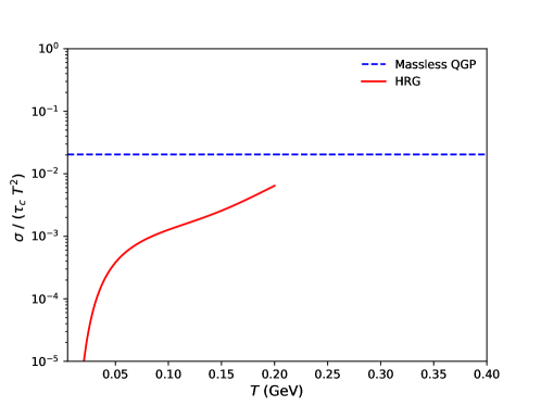
Figure 1: (Color online) Electrical conductivity $\sigma$ normalized by $\tau_{c}T^{2}$ as a function of $T$ for massless QGP and HRG.

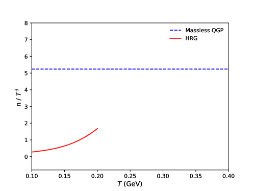
Figure 2: (Color online) Normalized number density $n/(T^{3})$ vs $T$ for massless QGP and HRG.

In Fig. 1, we have portrayed the normalized electrical conductivity $\sigma/\tau_{c}T^{2}$ with respect to temperature $T$. We take the help of Eq. 22 to get the expression of $\sigma_{\rm QGP}$ for massless QGP, which can be seen to be directly proportional to $\tau_{c}T^{2}$. Accordingly, we have obtained a horizontal line corresponding to $\sigma/\tau_{c}T^{2}=0.02$. For the hadronic temperature regime, we have presented the variation of scaled conductivity $\sigma/\tau_{c}T^{2}$ by resorting to the HRG model Eq. 15 at zero baryon chemical potential. For simplicity, we have assumed constant $\tau_{c}$ for all the hadrons to obtain the pattern of scaled $\sigma_{\rm HRG}$ in Fig. 1. The plot (red solid line) displays a sharp rise at low temperatures and eventually flattens as the temperature increases. The conductivity for the hadron gas obtained from the HRG model stays below the massless QGP (blue dashed line). The pattern is quite similar to the normalized thermodynamical quantities like pressure, energy density, etc, whose HRG estimations always remain below their massless QGP or Stefan-Boltzmann (SB) limits.

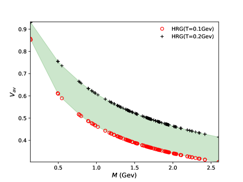
Figure 3: (Color online) Average velocity ($v_{\text{av}}$) as a function of hadron mass ($M$) for all hadrons at two different temperatures: $T$ = 0.1 GeV and T = 0.2 GeV.

In Fig. 2, we have compared the numerical magnitudes of normalized number density $\frac{n}{T^{3}}$ for massless QGP (red solid line) and hadron gas (blue dashed line). We use Eq. 24 and Eq. 18 for massless QGP and hadron gas for the determination of the magnitude of $\frac{n}{T^{3}}$. For QGP, owing to the relation $n\propto T^{3}$, we get a horizontal line at $\frac{n}{T^{3}}\approx 5.23$. In contrast, in the hadron gas, our model calculation produces a monotonically increasing $n$ or $n/T^{3}$ with respect to $T$. Again, we observe that, like conductivity, the number density value for hadron gas estimated from the HRG model stays below the massless QGP limit.

In Fig. 3, we have displayed the variation of the average velocity of different hadrons in the hadron gas with respect to their masses up to 2.6 GeV at two different temperatures: $T=0.1$ GeV and $T=0.2$ GeV. We have obtained the numerical values of $v_{\text{av}}$ from Eq. 17 at zero baryonic chemical potential. The result shows a decrease in average velocity $v_{\text{av}}$ of all the hadrons with respect to their masses. The lighter hadrons have high velocities compared to the heavier ones. An increase in temperature makes hadrons move with an increased velocity as the thermal energy increases with temperature. Moreover, we have also created a band to depict the range of velocity of all hadrons between $T=0.1$ GeV and $T=0.2$ GeV.

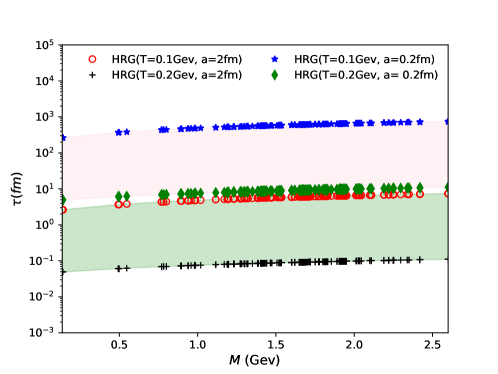
Figure 4: (Color online) Relaxation Time $\tau_{c}$ vs $M$ for various hadrons at two different temperatures: $T$ = 0.1 GeV and T = 0.2 GeV. Two different values of $a$ ($0.2$ fm and $2$ fm) are considered for each temperature.

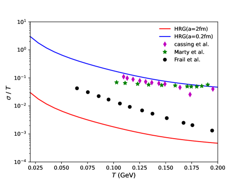
Figure 5: (Color online) Electrical conductivity $\sigma/T$ vs $T$ for HRG with temperature-dependent $\tau_{c}(T)$ at a = 0.2 and 2 fm and its comparison with the models of Cassing et al. [108], Marty et al. [109], Frail et al. [110].

In Fig. 4, we have illustrated the change of relaxation or collision time of different hadrons with respect to their masses for two different temperature values: $T=0.1$ GeV and $T=0.2$ GeV. For the evaluation of collision time, we have relied on the expression of the hard-sphere scattering model of the collision set down in Eq. 16. For each $T$ value, we take two different scattering lengths $a$ to display the variation of $\tau_{c}$ with respect to both $T$ and $a$. For a fixed $a$ the relaxation time $\tau_{c}(T)$ decreases because of the increase of $v_{\text{av}}(T)$ and $n(T)$ by following the Eq. 16. Similarly, for a given $T$, the relaxation time increases with $a$ since $\tau_{c}\propto\frac{1}{a^{2}}$. Here we have chosen $a=0.2$ fm and $a=2$ fm whose reason will be clear in Fig. 5.

Next, we have aimed to compile earlier estimated data of $\sigma/T$ within the hadronic temperature domain, where few selective estimated results [108, 109, 110] are shown in Fig. 5. The order of magnitude for $\sigma/T$, obtained by Cassing et al. [108] (Diamonds), Marty et al.  [109] (Stars), Fraile et al.  [110] (solid circles) are within the range $0.001$ to $0.1$. A long list of references [108, 109, 110, 111, 112, 113, 114, 115, 116, 117, 118, 119, 120, 121, 122] can be found for microscopic estimation of $\sigma/T$, whose order of magnitude will be located within $0.001$ to $0.1$ for hadronic temperature domain and $0.002$ to $0.3$ within quark temperature domain. Now, it can be seen that all the data obtained from earlier works within the hadronic temperature domain can be covered by altering $a$ from $0.2$ to $2$ fm. For this reason, the same range of $a$ has been considered in previous Fig. 4.

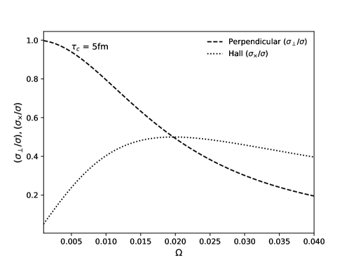
Figure 6: Perpendicular and Hall Electrical conductivity $\sigma_{\perp}/(\sigma)$, $\sigma_{\times}/(\sigma)$ vs $\Omega$ for HRG at $\tau_{c}=5$ fm and $T=0.150$ GeV.

Upto Fig. 5, we have gone through the estimations of $\sigma/T$ in the absence of rotation. In presence of rotation the isotropic nature of $\sigma/T$ converts into anistropic nature of $\sigma/T$, having multi components- $\sigma^{||}$, $\sigma^{\perp}$ and $\sigma^{\times}$. Interestingly, $\sigma^{||}$ in the presence of rotation is the same as $\sigma$, which is the isotropic conductivity in the absence of $\Omega$. The expression of $\sigma(T)$ given in Eq. 15 has two components: thermodynamical phase space and relaxation time $\tau_{c}(T)$. The former component has a non tunable temperature profile, while the latter component can be tunable by tuning the magnitude of scattering cross-section through $a$. We have used hard sphere scattering cross-section relation for the expression of $\tau_{c}(T)$, given in Eq. 16. The temperature dependance of $\tau_{c}$ is mainly determined by $n(T)$ and $v_{\rm av}(T)$ which are displayed in the earlier Figs. 2 and 3. After calibrating our results without rotation with earlier estimations, we will now proceed to apply them to rotating hadronic matter.

In Fig. 6, we have depicted the variation of perpendicular and hall conductivities $\sigma^{\perp,\times}$ normalized by the parallel conductivity $\sigma^{||}=\sigma$ as a function of $\Omega$ for a fixed $T=0.150$ GeV. We have employed Eq. 19,20 and 15 for the numerical estimation of $\sigma^{\perp}$, $\sigma^{\times}$ and $\sigma$ respectively for rotating HRG. In relation to Eq. 16 and Fig. 4, it is apparent that the relaxation time is a function of $a$, $T$, and $M$, i.e., $\tau_{c}=\tau_{c}(a,M,T)$. So, for a specific hadron in the system at a given temperature, it depends on the effective hard sphere scattering length. In the beginning, let us consider a constant $\tau_{c}$ for estimating $\sigma^{||,\perp,\times}$ instead of the actual $\tau_{c}(a,M,T)$. By doing this, we can visualize only the thermodynamical phase space part of $\sigma^{||,\perp,\times}(T,\Omega)$. In this plot, we choose a value of $\tau_{c}=5$ fm (25 GeV^-1), which falls in the band of $\tau_{c}$ obtained in Fig. 4 for $a=2$ fm. In HICs, the average value of the local vorticity can be taken as a measure of the global vorticity or angular velocity of the system. The average vorticity for HIC has been calculated from various models [22, 123, 55, 56]. Inspired by these studies, we choose the scale of the $\Omega$ axis from $0-0.04$ GeV. $\sigma^{\perp}$ (or $\sigma^{0}$), the perpendicular conductivity of the rotating HRG corresponds to the current in the direction of the applied electric field in the $XY$ plane. In the limit of $\Omega\xrightarrow{}0$, $\sigma^{\perp}$ reduces to conductivity $\sigma$. In our plot, this feature can be seen where $\frac{\sigma^{\perp}}{\sigma}\xrightarrow{}1$ as one approach to $\Omega\xrightarrow{}0$. Similarly, we can see the matrix in Eqn. 14 that $\sigma^{1}\equiv\sigma^{\times}$ drives the electric current in the XY-plane of the rotating hadron gas; it drives current in the $X$-direction if the electric field is in the $Y$-direction and vice-versa. In the limit $\Omega\xrightarrow{}0$, $\sigma^{\times}$ vanishes. The Hall conductivity $\sigma^{\times}$ shows interesting characteristics, it first increases with $\Omega$ to hit a peak where $\tau_{\Omega}\equiv\frac{1}{2\Omega}$ approaches $\tau_{c}$ and then decreases with further increase in $\Omega$. From Fig.6 one can notice that, for slowly rotating HRG, i.e., at low $\Omega$, the $\sigma^{\perp}$ dominates over $\sigma^{\times}$ whereas, for a fastly rotating HRG, i.e., at high $\Omega$ we see that $\sigma^{\perp}<\sigma^{\times}$. Noticeably, the magnitude of $\sigma^{\perp,\times}/\sigma$ in the figure lies below one, i.e., $\sigma^{\perp,\times}/\sigma\leq 1$. This property can be understood by recognizing three different time scales associated with the rotating hadronic gas: $\tau_{c}\equiv\tau^{||}_{c}$, $\tau^{\perp}_{c}$ and $\tau^{\times}_{c}$. The effective relaxation times $\tau^{\perp}_{c}$ and $\tau^{\times}_{c}$ occurs in the mathematical expression of $\sigma^{\perp}$ and $\sigma^{\times}$ are given below,

$$\tau^{\perp}_{c}=\frac{\tau_{c}}{1+\big{(}\frac{\tau_{c}}{\tau_{\Omega}}\big{)}^{2}},$$

$$\tau^{\times}_{c}=\frac{\tau_{c}\big{(}\frac{\tau_{c}}{\tau_{\Omega}}\big{)}}{1+\big{(}\frac{\tau_{c}}{\tau_{\Omega}}\big{)}^{2}}.$$

A glance at the above time scales suggests that $\tau^{\perp}_{c}<\tau_{c}$ and $\tau^{\times}_{c}<\tau_{c}$ which determines the ordering $\sigma^{\perp}<\sigma$ and $\sigma^{\times}<\sigma$.

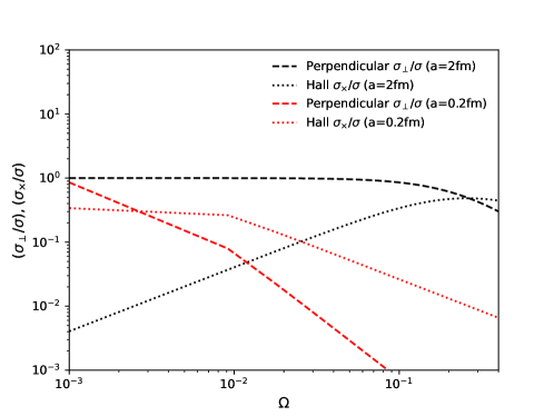
Figure 7: (Color online) Perpendicular and Hall Electrical conductivity ($\sigma_{\perp}/\sigma,\sigma_{\times}/\sigma$) vs $\Omega$ for HRG at T=0.150 ${\rm~{}GeV}$.

We have delineated the variation of normalized conductivity $\frac{\sigma^{\perp,\times}}{\sigma}$ in relation to the angular velocity $\Omega$ of the hadronic medium at $T=0.150$ GeV in Fig. 7. In contrast to Fig. 6, where we have interpreted the alternation of $\frac{\sigma^{\perp,\times}}{\sigma}$ graphically for a fixed value of $\tau_{c}=5$ fm, we take here the individual $\tau_{c}$ of the rotating hadrons by using Eq. 16. For fixed $T=0.150$ GeV and take two different values $a=(0.2~{}{\rm fm},2~{}{\rm fm})$ we have calculated $\tau_{c}=\tau_{c}(a,M,T)$ for different hadron resonances with mass $M$. The different values of $a$ have chosen here are the tuned scattering lengths obtained by the calibration done in Fig. 5. For the value of $a=2$ fm, we see that for a rotating HRG with $\Omega$ in the range $0.001$ GeV to $0.02$ GeV, the $\sigma^{\perp}$ is almost equal to $\sigma$ and $\sigma^{\times}$ is negligible. This suggests an almost isotropic HRG with the scattering length $a=2$ fm. Nevertheless, for $a=0.2$ fm, we observe that in the range $\Omega=0.01-0.02$ GeV there is a significant magnitude of $\sigma^{\times}$ which is around $10$ to $15$ % of $\sigma$. Also, in the same range of $\Omega$, one can notice a significant suppression of the $\sigma^{\perp}$ with respect to $\sigma$, which is around $90\%$. This suggests a highly anisotropic HRG with a hugely suppressed perpendicular conductivity $\sigma^{\perp}$ along with a large magnitude of hall conductivity $\sigma^{\times}$.

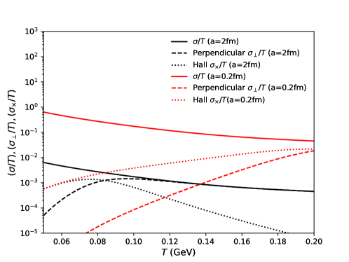
Figure 8: (Color online) Parallel, perpendicular, and Hall electrical conductivity ($\sigma/T$, $\sigma_{\perp}/T$, $\sigma_{\times}/T$) as functions of temperature ($T$) for HRG with $\tau_{c}(T)$ and $\tau_{\Omega}=6$ fm.

In Fig. 8, we have displayed the temperature dependence of the scaled conductivities $\sigma/T$ for the rotating HRG at an angular speed $\Omega=0.016$ GeV ($\tau_{\Omega}\approx 6$ fm). Similar to the previous figure, we take two different values of $a~{}(0.2~{}{\rm fm},2~{}{\rm fm})$ for the determination of $\tau_{c}(a,M,T)$ from Eq. 16. The plot represents a strong variation of both perpendicular $\sigma^{\perp}$ and hall $\sigma^{\times}$ conductivities in relation to temperature $T$. For a rotating HRG with $a=2$ fm, the $\sigma^{\perp}$ almost merges with $\sigma$ for temperature $T\geq 0.12$ GeV. This implies an almost isotropic rotating HRG with $\sigma^{\perp}\approx\sigma$. Nevertheless, one can define a region of temperature $T=0.05-0.14$ GeV where the system still has a significant magnitude of $\sigma^{\times}$ with $\sigma/\sigma^{\times}\sim 10$ or less. On the other hand, in a rotating HRG with $a=0.2$ fm, there is a remarkable suppression of $\sigma^{\perp}$ with respect to $\sigma$ in the $T$ range $0.10-0.20$ GeV. The magnitude of the suppression is around $90\%$ at $T=0.12$ GeV. These observations suggest strongly anisotropic rotating HRG with $a=0.2$ fm. There is also a significant magnitude of hall conductivity $\sigma^{\times}$ for $T$ more than $0.14$ GeV, i.e., $\sigma^{\times}/\sigma\geq 10$ for $T\geq 0.14$ GeV.

At the end, we can find a summarized and qualitative message from our detailed quantitative investigations. It says that Coriolis force can have a noticeable impact on creating an anisotropic conductivity tensor at a finite rotation of the HRG system, as done by the Lorentz force at a finite magnetic field. However, this noticeable impact will quantitatively depend on the hadronic scattering strengths, quantified by $a$ in our study. We have shown the noticeable and non-noticeable impact for $a=0.2$ fm and $a=2$ fm, respectively. Another debatable point is that how fast or slow the angular velocity will decay with time [56, 55, 22] so that hadronic matter will face it. In this context, a possibility of noticeable impact for any values within the range $\Omega=0.001-0.02$ GeV can be found.

IV Summary

In this work, we have made an effort to visualize the effect of Coriolis force on electrical conductivity in the Hadron Resonance Gas Model. The coefficient of proportionality between electrical current density and electrical field is known as electrical conductivity. Using the Boltzmann transport equation and the relaxation time approximation, we have calculated their microscopic expressions within the framework of kinetic theory based on their macroscopic formulations. The Coriolis force in rotating frames leads to similar anisotropy in the electrical conductivity tensor ($\sigma$) as the Lorentz force introduced in the presence of a magnetic field. The generated anisotropy is categorized into three parts: the Hall, perpendicular, and parallel components. The parallel component of electrical conductivity remains unaffected as it is independent of the relaxation time of the medium. However, we observe the variations in the scaled electrical conductivity of the perpendicular and Hall components with temperature in the presence of Coriolis force. In the absence of rotation, the scaled electrical conductivity (scaled with $\tau_{c}T^{2}$) increases with temperature but stays below the results obtained for massless QGP or Stefan-Boltzmann (SB) limits similar to the normalized thermodynamical quantities like pressure, energy density, etc. The average velocity of particles decreases monotonically with mass, which leads to an increase in particle relaxation time as a function of their respective masses. We estimate the relaxation time using the hard-sphere scattering model. We observed that the earlier estimations of ($\sigma/T$) could be tuned by varying the scattering lengths $a$ from 0.2 fm to 2 fm. A monotonic decreasing trend is observed in electrical conductivity with temperature in the absence of rotation. The presence of the Coriolis force induces an anisotropic nature in electrical conductivity. We observed that as the angular velocity ($\Omega$) of the rotating hadron gas system increases, the perpendicular component of electrical conductivity decreases. As the rotation speed ($\Omega$) approaches zero, the perpendicular component converges to the overall conductivity $\sigma$. On the contrary, the Hall component vanishes towards small $\Omega$. The Hall component shows interesting behavior; initially, it increases with $\Omega$, reaching a peak when the characteristic rotation time ($\tau_{\Omega}$) becomes comparable to the relaxation time $\tau_{c}$ and then decreases with further increase in $\Omega$. Therefore, we can conclude that in a slowly rotating HRG, with low $\Omega$, $\sigma^{\perp}$ dominates over the Hall conductivity $\sigma^{\times}$, whereas, for a fastly rotating (large $\Omega$) HRG $\sigma^{\times}>\sigma^{\perp}$. Even more interestingly, we observe that this flip from $\sigma^{\perp}$ dominance to $\sigma^{\times}$ dominance occurs at relatively smaller angular velocities for systems with smaller scattering lengths. In the end, we estimate the variation of electrical conductivity components with temperature at a fixed angular speed. We observed a strong variation in both perpendicular and Hall components with temperature. With the chosen angular speed $\Omega=0.016$ GeV ($\tau_{\Omega}\approx 6$ fm) the $\sigma^{\perp}$ almost merges with $\sigma$ above for temperature $T\approx 0.12$ GeV for $a=2$ fm. This implies an almost isotropic rotating HRG with $\sigma^{\perp}\approx\sigma$. On the other hand, for $a=0.2$ fm, suppression of $\sigma^{\perp}$ with respect to $\sigma$ is notably strong up to $T\approx 0.20$ GeV, which suggests strongly anisotropic rotating HRG with $a=0.2$ fm.

V Acknowledgement

NP and AD gratefully acknowledge the Ministry of Education (MoE), Govt. of India. The authors extend their thanks to Snigdha Ghosh for sharing valuable materials and insights on HRG model calculations.

References

- Adamczyk et al. [2017] L. Adamczyk et al. (STAR), Global hyperon polarization in nuclear collisions: evidence for the most vortical fluid, Nature 548, 62 (2017), arXiv:1701.06657 [nucl-ex] .
- Liang and Wang [2005a] Z.-T. Liang and X.-N. Wang, Globally polarized quark-gluon plasma in non-central A+A collisions, Phys. Rev. Lett. 94, 102301 (2005a), [Erratum: Phys.Rev.Lett. 96, 039901 (2006)], arXiv:nucl-th/0410079 .
- Becattini et al. [2008] F. Becattini, F. Piccinini, and J. Rizzo, Angular momentum conservation in heavy ion collisions at very high energy, Phys. Rev. C 77, 024906 (2008), arXiv:0711.1253 [nucl-th] .
- Adam et al. [2018] J. Adam et al. (STAR), Global polarization of hyperons in Au+Au collisions at = 200 GeV, Phys. Rev. C 98, 014910 (2018), arXiv:1805.04400 [nucl-ex] .
- Acharya et al. [2020] S. Acharya et al. (ALICE), Evidence of Spin-Orbital Angular Momentum Interactions in Relativistic Heavy-Ion Collisions, Phys. Rev. Lett. 125, 012301 (2020), arXiv:1910.14408 [nucl-ex] .
- Abdallah et al. [2023] M. S. Abdallah et al. (STAR), Pattern of global spin alignment of and K∗0 mesons in heavy-ion collisions, Nature 614, 244 (2023), arXiv:2204.02302 [hep-ph] .
- Acharya et al. [2023] S. Acharya et al. (ALICE), Measurement of the J/ Polarization with Respect to the Event Plane in Pb-Pb Collisions at the LHC, Phys. Rev. Lett. 131, 042303 (2023), arXiv:2204.10171 [nucl-ex] .
- Becattini and Piccinini [2008] F. Becattini and F. Piccinini, The ideal relativistic spinning gas: Polarization and spectra, Annals of Physics 323, 2452 (2008).
- Becattini et al. [2013a] F. Becattini, V. Chandra, L. Del Zanna, and E. Grossi, Relativistic distribution function for particles with spin at local thermodynamical equilibrium, Annals Phys. 338, 32 (2013a), arXiv:1303.3431 [nucl-th] .
- Becattini et al. [2013b] F. Becattini, L. Csernai, and D. J. Wang, polarization in peripheral heavy ion collisions, Phys. Rev. C 88, 034905 (2013b), [Erratum: Phys.Rev.C 93, 069901 (2016)], arXiv:1304.4427 [nucl-th] .
- Betz et al. [2007] B. Betz, M. Gyulassy, and G. Torrieri, Polarization probes of vorticity in heavy ion collisions, Phys. Rev. C 76, 044901 (2007), arXiv:0708.0035 [nucl-th] .
- Liang and Wang [2005b] Z.-T. Liang and X.-N. Wang, Spin alignment of vector mesons in non-central a+a collisions, Physics Letters B 629, 20 (2005b).
- Gao et al. [2008] J.-H. Gao, S.-W. Chen, W.-t. Deng, Z.-T. Liang, Q. Wang, and X.-N. Wang, Global quark polarization in noncentral collisions, Phys. Rev. C 77, 044902 (2008).
- Huang et al. [2011] X.-G. Huang, P. Huovinen, and X.-N. Wang, Quark polarization in a viscous quark-gluon plasma, Phys. Rev. C 84, 054910 (2011).
- Becattini et al. [2021] F. Becattini, M. Buzzegoli, and A. Palermo, Spin-thermal shear coupling in a relativistic fluid, Phys. Lett. B 820, 136519 (2021), arXiv:2103.10917 [nucl-th] .
- Xia et al. [2018] X.-L. Xia, H. Li, Z.-B. Tang, and Q. Wang, Probing vorticity structure in heavy-ion collisions by local polarization, Phys. Rev. C 98, 024905 (2018), arXiv:1803.00867 [nucl-th] .
- Florkowski et al. [2018a] W. Florkowski, B. Friman, A. Jaiswal, and E. Speranza, Relativistic fluid dynamics with spin, Phys. Rev. C 97, 041901 (2018a).
- Florkowski et al. [2018b] W. Florkowski, B. Friman, A. Jaiswal, R. Ryblewski, and E. Speranza, Spin-dependent distribution functions for relativistic hydrodynamics of spin- particles, Phys. Rev. D 97, 116017 (2018b).
- Florkowski et al. [2019a] W. Florkowski, A. Kumar, R. Ryblewski, and R. Singh, Spin polarization evolution in a boost invariant hydrodynamical background, Phys. Rev. C 99, 044910 (2019a), arXiv:1901.09655 [hep-ph] .
- Wei et al. [2019] D.-X. Wei, W.-T. Deng, and X.-G. Huang, Thermal vorticity and spin polarization in heavy-ion collisions, Phys. Rev. C 99, 014905 (2019), arXiv:1810.00151 [nucl-th] .
- Wu et al. [2021] H.-Z. Wu, L.-G. Pang, X.-G. Huang, and Q. Wang, Local Spin Polarization in 200 GeV Au+Au and 2.76 TeV Pb+Pb Collisions, Nucl. Phys. A 1005, 121831 (2021), arXiv:2002.03360 [nucl-th] .
- Huang et al. [2021] X.-G. Huang, J. Liao, Q. Wang, and X.-L. Xia, Vorticity and Spin Polarization in Heavy Ion Collisions: Transport Models, Lect. Notes Phys. 987, 281 (2021), arXiv:2010.08937 [nucl-th] .
- Fu et al. [2021] B. Fu, S. Y. F. Liu, L. Pang, H. Song, and Y. Yin, Shear-Induced Spin Polarization in Heavy-Ion Collisions, Phys. Rev. Lett. 127, 142301 (2021), arXiv:2103.10403 [hep-ph] .
- Deng et al. [2022] X.-G. Deng, X.-G. Huang, and Y.-G. Ma, Lambda polarization in 108ag+108ag and 197au+197au collisions around a few gev, Physics Letters B 835, 137560 (2022).
- Li et al. [2022] H. Li, X.-L. Xia, X.-G. Huang, and H. Z. Huang, Global spin polarization of multistrange hyperons and feed-down effect in heavy-ion collisions, Physics Letters B 827, 136971 (2022).
- Gao et al. [2012] J.-H. Gao, Z.-T. Liang, S. Pu, Q. Wang, and X.-N. Wang, Chiral anomaly and local polarization effect from the quantum kinetic approach, Phys. Rev. Lett. 109, 232301 (2012).
- Chen et al. [2013] J.-W. Chen, S. Pu, Q. Wang, and X.-N. Wang, Berry curvature and four-dimensional monopoles in the relativistic chiral kinetic equation, Phys. Rev. Lett. 110, 262301 (2013).
- Fang et al. [2016] R.-h. Fang, L.-g. Pang, Q. Wang, and X.-n. Wang, Polarization of massive fermions in a vortical fluid, Phys. Rev. C 94, 024904 (2016).
- Fang et al. [2017] R.-h. Fang, J.-y. Pang, Q. Wang, and X.-n. Wang, Pseudoscalar condensation induced by chiral anomaly and vorticity for massive fermions, Phys. Rev. D 95, 014032 (2017).
- hua Gao and Wang [2015] J. hua Gao and Q. Wang, Magnetic moment, vorticity-spin coupling and parity-odd conductivity of chiral fermions in 4-dimensional wigner functions, Physics Letters B 749, 542 (2015).
- Hidaka et al. [2017] Y. Hidaka, S. Pu, and D.-L. Yang, Relativistic chiral kinetic theory from quantum field theories, Phys. Rev. D 95, 091901 (2017).
- Gao et al. [2017] J.-h. Gao, S. Pu, and Q. Wang, Covariant chiral kinetic equation in the wigner function approach, Phys. Rev. D 96, 016002 (2017).
- Gao et al. [2018] J.-H. Gao, Z.-T. Liang, Q. Wang, and X.-N. Wang, Disentangling covariant wigner functions for chiral fermions, Phys. Rev. D 98, 036019 (2018).
- Huang et al. [2018] A. Huang, S. Shi, Y. Jiang, J. Liao, and P. Zhuang, Complete and consistent chiral transport from wigner function formalism, Phys. Rev. D 98, 036010 (2018).
- Gao et al. [2019] J.-H. Gao, J.-Y. Pang, and Q. Wang, Chiral vortical effect in wigner function approach, Phys. Rev. D 100, 016008 (2019).
- Gao and Liang [2019] J.-H. Gao and Z.-T. Liang, Relativistic quantum kinetic theory for massive fermions and spin effects, Phys. Rev. D 100, 056021 (2019).
- Hattori et al. [2019] K. Hattori, Y. Hidaka, and D.-L. Yang, Axial kinetic theory and spin transport for fermions with arbitrary mass, Phys. Rev. D 100, 096011 (2019).
- Wang et al. [2019] Z. Wang, X. Guo, S. Shi, and P. Zhuang, Mass correction to chiral kinetic equations, Phys. Rev. D 100, 014015 (2019).
- Weickgenannt et al. [2019] N. Weickgenannt, X.-l. Sheng, E. Speranza, Q. Wang, and D. H. Rischke, Kinetic theory for massive particles from the wigner-function formalism, Phys. Rev. D 100, 056018 (2019).
- Yang et al. [2020] D.-L. Yang, K. Hattori, and Y. Hidaka, Effective quantum kinetic theory for spin transport of fermions with collsional effects, Journal of High Energy Physics 2020, 1 (2020).
- Weickgenannt et al. [2021a] N. Weickgenannt, E. Speranza, X.-l. Sheng, Q. Wang, and D. H. Rischke, Generating spin polarization from vorticity through nonlocal collisions, Phys. Rev. Lett. 127, 052301 (2021a).
- Weickgenannt et al. [2021b] N. Weickgenannt, E. Speranza, X.-l. Sheng, Q. Wang, and D. H. Rischke, Derivation of the nonlocal collision term in the relativistic boltzmann equation for massive spin- particles from quantum field theory, Phys. Rev. D 104, 016022 (2021b).
- Becattini and Ferroni [2007] F. Becattini and L. Ferroni, The microcanonical ensemble of the ideal relativistic quantum gas with angular momentum conservation, The European Physical Journal C 52, 597 (2007).
- Becattini and Tinti [2010] F. Becattini and L. Tinti, The ideal relativistic rotating gas as a perfect fluid with spin, Annals of Physics 325, 1566 (2010).
- Becattini et al. [2015] F. Becattini, G. Inghirami, V. Rolando, A. Beraudo, L. Del Zanna, A. De Pace, M. Nardi, G. Pagliara, and V. Chandra, A study of vorticity formation in high energy nuclear collisions, Eur. Phys. J. C 75, 406 (2015), [Erratum: Eur.Phys.J.C 78, 354 (2018)], arXiv:1501.04468 [nucl-th] .
- Chen et al. [2009] S.-w. Chen, J. Deng, J.-h. Gao, and Q. Wang, A general derivation of differential cross section in quark-quark and quark-gluon scatterings at fixed impact parameter, Frontiers of Physics in China 4, 509 (2009).
- Becattini [2011] F. Becattini, Hydrodynamics of fluids with spin, Physics of Particles and Nuclei Letters 8, 801 (2011).
- Florkowski et al. [2019b] W. Florkowski, A. Kumar, and R. Ryblewski, Relativistic hydrodynamics for spin-polarized fluids, Prog. Part. Nucl. Phys. 108, 103709 (2019b), arXiv:1811.04409 [nucl-th] .
- Florkowski et al. [2018c] W. Florkowski, A. Kumar, and R. Ryblewski, Thermodynamic versus kinetic approach to polarization-vorticity coupling, Phys. Rev. C 98, 044906 (2018c), arXiv:1806.02616 [hep-ph] .
- Becattini et al. [2019] F. Becattini, W. Florkowski, and E. Speranza, Spin tensor and its role in non-equilibrium thermodynamics, Physics Letters B 789, 419 (2019).
- Bhadury et al. [2021a] S. Bhadury, W. Florkowski, A. Jaiswal, A. Kumar, and R. Ryblewski, Relativistic dissipative spin dynamics in the relaxation time approximation, Physics Letters B 814, 136096 (2021a).
- Bhadury et al. [2021b] S. Bhadury, W. Florkowski, A. Jaiswal, A. Kumar, and R. Ryblewski, Dissipative spin dynamics in relativistic matter, Phys. Rev. D 103, 014030 (2021b).
- Daher et al. [2022] A. Daher, A. Das, W. Florkowski, and R. Ryblewski, Equivalence of canonical and phenomenological formulations of spin hydrodynamics, arXiv preprint arXiv:2202.12609 (2022).
- Bhadury et al. [2022] S. Bhadury, W. Florkowski, A. Jaiswal, A. Kumar, and R. Ryblewski, Relativistic spin magnetohydrodynamics, Phys. Rev. Lett. 129, 192301 (2022).
- Deng and Huang [2016] W.-T. Deng and X.-G. Huang, Vorticity in Heavy-Ion Collisions, Phys. Rev. C 93, 064907 (2016), arXiv:1603.06117 [nucl-th] .
- Jiang et al. [2016] Y. Jiang, Z.-W. Lin, and J. Liao, Rotating quark-gluon plasma in relativistic heavy-ion collisions, Phys. Rev. C 94, 044910 (2016).
- Pang et al. [2016] L.-G. Pang, H. Petersen, Q. Wang, and X.-N. Wang, Vortical Fluid and Spin Correlations in High-Energy Heavy-Ion Collisions, Phys. Rev. Lett. 117, 192301 (2016), arXiv:1605.04024 [hep-ph] .
- Li et al. [2017] H. Li, L.-G. Pang, Q. Wang, and X.-L. Xia, Global polarization in heavy-ion collisions from a transport model, Phys. Rev. C 96, 054908 (2017), arXiv:1704.01507 [nucl-th] .
- Huang [2021] X.-G. Huang, Vorticity and Spin Polarization — A Theoretical Perspective, Nucl. Phys. A 1005, 121752 (2021), arXiv:2002.07549 [nucl-th] .
- Pradhan et al. [2023a] K. K. Pradhan, B. Sahoo, D. Sahu, and R. Sahoo, Thermodynamics of a rotating hadron resonance gas with van der Waals interaction, (2023a), arXiv:2304.05190 [hep-ph] .
- Sahoo et al. [2023] B. Sahoo, C. R. Singh, D. Sahu, R. Sahoo, and J.-e. Alam, Impact of vorticity and viscosity on the hydrodynamic evolution of hot QCD medium, Eur. Phys. J. C 83, 873 (2023), arXiv:2302.07668 [hep-ph] .
- Mukherjee et al. [2024] G. Mukherjee, D. Dutta, and D. K. Mishra, Conserved number fluctuations under global rotation in a hadron resonance gas model, Eur. Phys. J. C 84, 258 (2024), arXiv:2304.14658 [hep-ph] .
- Chernodub [2021] M. N. Chernodub, Inhomogeneous confining-deconfining phases in rotating plasmas, Phys. Rev. D 103, 054027 (2021), arXiv:2012.04924 [hep-ph] .
- Chernodub and Gongyo [2017] M. N. Chernodub and S. Gongyo, Effects of rotation and boundaries on chiral symmetry breaking of relativistic fermions, Phys. Rev. D 95, 096006 (2017), arXiv:1702.08266 [hep-th] .
- Braguta et al. [2023] V. V. Braguta, M. N. Chernodub, A. A. Roenko, and D. A. Sychev, Negative moment of inertia and rotational instability of gluon plasma, (2023), arXiv:2303.03147 [hep-lat] .
- Chernodub et al. [2023] M. N. Chernodub, V. A. Goy, and A. V. Molochkov, Inhomogeneity of a rotating gluon plasma and the Tolman-Ehrenfest law in imaginary time: Lattice results for fast imaginary rotation, Phys. Rev. D 107, 114502 (2023), arXiv:2209.15534 [hep-lat] .
- Sivardiere [1983] J. Sivardiere, On the analogy between inertial and electromagnetic forces, European Journal of Physics 4, 162 (1983).
- Johnson [2000] B. L. Johnson, Inertial forces and the hall effect, Am. J. Phys. 68, 649 (2000).
- Sakurai [1980] J. J. Sakurai, Comments on quantum-mechanical interference due to the earth’s rotation, Phys. Rev. D 21, 2993 (1980).
- Dey et al. [2021a] J. Dey, S. Satapathy, P. Murmu, and S. Ghosh, Shear viscosity and electrical conductivity of the relativistic fluid in the presence of a magnetic field: A massless case, Pramana 95, 125 (2021a), arXiv:1907.11164 [hep-ph] .
- Dash et al. [2020] A. Dash, S. Samanta, J. Dey, U. Gangopadhyaya, S. Ghosh, and V. Roy, Anisotropic transport properties of a hadron resonance gas in a magnetic field, Phys. Rev. D 102, 016016 (2020), arXiv:2002.08781 [nucl-th] .
- Dey et al. [2022] J. Dey, S. Samanta, S. Ghosh, and S. Satapathy, Quantum expression for the electrical conductivity of massless quark matter and of the hadron resonance gas in the presence of a magnetic field, Phys. Rev. C 106, 044914 (2022), arXiv:2002.04434 [nucl-th] .
- Ghosh et al. [2020] S. Ghosh, A. Bandyopadhyay, R. L. S. Farias, J. Dey, and G. a. Krein, Anisotropic electrical conductivity of magnetized hot quark matter, Phys. Rev. D 102, 114015 (2020), arXiv:1911.10005 [hep-ph] .
- Dey et al. [2021b] J. Dey, S. Satapathy, A. Mishra, S. Paul, and S. Ghosh, From noninteracting to interacting picture of quark–gluon plasma in the presence of a magnetic field and its fluid property, Int. J. Mod. Phys. E 30, 2150044 (2021b), arXiv:1908.04335 [hep-ph] .
- Kalikotay et al. [2020] P. Kalikotay, S. Ghosh, N. Chaudhuri, P. Roy, and S. Sarkar, Medium effects on the electrical and Hall conductivities of a hot and magnetized pion gas, Phys. Rev. D 102, 076007 (2020), arXiv:2009.10493 [hep-ph] .
- Dey et al. [2023] J. Dey, A. Bandyopadhyay, A. Gupta, N. Pujari, and S. Ghosh, Electrical conductivity of strongly magnetized dense quark matter - possibility of quantum Hall effect, Nucl. Phys. A 1034, 122654 (2023), arXiv:2103.15364 [hep-ph] .
- Satapathy et al. [2021] S. Satapathy, S. Ghosh, and S. Ghosh, Kubo estimation of the electrical conductivity for a hot relativistic fluid in the presence of a magnetic field, Phys. Rev. D 104, 056030 (2021), arXiv:2104.03917 [hep-ph] .
- Das et al. [2019] A. Das, H. Mishra, and R. K. Mohapatra, Electrical conductivity and Hall conductivity of a hot and dense hadron gas in a magnetic field: A relaxation time approach, Phys. Rev. D 99, 094031 (2019), arXiv:1903.03938 [hep-ph] .
- Das et al. [2020] A. Das, H. Mishra, and R. K. Mohapatra, Electrical conductivity and Hall conductivity of a hot and dense quark gluon plasma in a magnetic field: A quasiparticle approach, Phys. Rev. D 101, 034027 (2020), arXiv:1907.05298 [hep-ph] .
- Chatterjee et al. [2021] B. Chatterjee, R. Rath, G. Sarwar, and R. Sahoo, Centrality dependence of Electrical and Hall conductivity at RHIC and LHC energies for a Conformal System, Eur. Phys. J. A 57, 45 (2021), arXiv:1908.01121 [hep-ph] .
- Hattori and Satow [2016] K. Hattori and D. Satow, Electrical Conductivity of Quark-Gluon Plasma in Strong Magnetic Fields, Phys. Rev. D 94, 114032 (2016), arXiv:1610.06818 [hep-ph] .
- Hattori et al. [2017] K. Hattori, S. Li, D. Satow, and H.-U. Yee, Longitudinal Conductivity in Strong Magnetic Field in Perturbative QCD: Complete Leading Order, Phys. Rev. D 95, 076008 (2017), arXiv:1610.06839 [hep-ph] .
- Satapathy et al. [2022] S. Satapathy, S. Ghosh, and S. Ghosh, Quantum field theoretical structure of electrical conductivity of cold and dense fermionic matter in the presence of a magnetic field, Phys. Rev. D 106, 036006 (2022), arXiv:2112.08236 [hep-ph] .
- Aung et al. [2024] C. W. Aung, A. Dwibedi, J. Dey, and S. Ghosh, Effect of Coriolis force on the shear viscosity of quark matter: A nonrelativistic description, Phys. Rev. C 109, 034913 (2024), arXiv:2303.16462 [nucl-th] .
- Dwibedi et al. [2024] A. Dwibedi, C. W. Aung, J. Dey, and S. Ghosh, Effect of the Coriolis force on the electrical conductivity of quark matter: A nonrelativistic description, Phys. Rev. C 109, 034914 (2024), arXiv:2305.10183 [nucl-th] .
- Dashen et al. [1969] R. Dashen, S.-K. Ma, and H. J. Bernstein, S Matrix formulation of statistical mechanics, Phys. Rev. 187, 345 (1969).
- Dashen and Rajaraman [1974] R. F. Dashen and R. Rajaraman, Narrow Resonances in Statistical Mechanics, Phys. Rev. D 10, 694 (1974).
- Karsch et al. [2003] F. Karsch, K. Redlich, and A. Tawfik, Thermodynamics at nonzero baryon number density: A Comparison of lattice and hadron resonance gas model calculations, Phys. Lett. B 571, 67 (2003), arXiv:hep-ph/0306208 .
- Braun-Munzinger et al. [2016] P. Braun-Munzinger, V. Koch, T. Schäfer, and J. Stachel, Properties of hot and dense matter from relativistic heavy ion collisions, Phys. Rept. 621, 76 (2016), arXiv:1510.00442 [nucl-th] .
- Begun et al. [2006] V. V. Begun, M. I. Gorenstein, M. Hauer, V. P. Konchakovski, and O. S. Zozulya, Multiplicity Fluctuations in Hadron-Resonance Gas, Phys. Rev. C 74, 044903 (2006), arXiv:nucl-th/0606036 .
- Nahrgang et al. [2015] M. Nahrgang, M. Bluhm, P. Alba, R. Bellwied, and C. Ratti, Impact of resonance regeneration and decay on the net-proton fluctuations in a hadron resonance gas, Eur. Phys. J. C 75, 573 (2015), arXiv:1402.1238 [hep-ph] .
- Bazavov et al. [2012] A. Bazavov et al. (HotQCD), Fluctuations and Correlations of net baryon number, electric charge, and strangeness: A comparison of lattice QCD results with the hadron resonance gas model, Phys. Rev. D 86, 034509 (2012), arXiv:1203.0784 [hep-lat] .
- Bhattacharyya et al. [2014] A. Bhattacharyya, S. Das, S. K. Ghosh, R. Ray, and S. Samanta, Fluctuations and correlations of conserved charges in an excluded volume hadron resonance gas model, Phys. Rev. C 90, 034909 (2014), arXiv:1310.2793 [hep-ph] .
- Chatterjee et al. [2016] A. Chatterjee, S. Chatterjee, T. K. Nayak, and N. R. Sahoo, Diagonal and off-diagonal susceptibilities of conserved quantities in relativistic heavy-ion collisions, J. Phys. G 43, 125103 (2016), arXiv:1606.09573 [nucl-ex] .
- Gorenstein et al. [2008] M. I. Gorenstein, M. Hauer, and O. N. Moroz, Viscosity in the excluded volume hadron gas model, Phys. Rev. C 77, 024911 (2008), arXiv:0708.0137 [nucl-th] .
- Noronha-Hostler et al. [2012] J. Noronha-Hostler, J. Noronha, and C. Greiner, Hadron Mass Spectrum and the Shear Viscosity to Entropy Density Ratio of Hot Hadronic Matter, Phys. Rev. C 86, 024913 (2012), arXiv:1206.5138 [nucl-th] .
- Tiwari et al. [2012] S. K. Tiwari, P. K. Srivastava, and C. P. Singh, Description of Hot and Dense Hadron Gas Properties in a New Excluded-Volume model, Phys. Rev. C 85, 014908 (2012), arXiv:1111.2406 [hep-ph] .
- Pradhan et al. [2023b] K. K. Pradhan, D. Sahu, R. Scaria, and R. Sahoo, Conductivity, diffusivity, and violation of the Wiedemann-Franz Law in a hadron resonance gas with van der Waals interactions, Phys. Rev. C 107, 014910 (2023b), arXiv:2205.03149 [hep-ph] .
- Noronha-Hostler et al. [2009] J. Noronha-Hostler, J. Noronha, and C. Greiner, Transport Coefficients of Hadronic Matter near T(c), Phys. Rev. Lett. 103, 172302 (2009), arXiv:0811.1571 [nucl-th] .
- Kadam and Mishra [2014] G. P. Kadam and H. Mishra, Bulk and shear viscosities of hot and dense hadron gas, Nucl. Phys. A 934, 133 (2014), arXiv:1408.6329 [hep-ph] .
- Zhang et al. [2020] H.-X. Zhang, J.-W. Kang, and B.-W. Zhang, In-medium effect on the thermodynamics and transport coefficients in the van der Waals hadron resonance gas, Phys. Rev. D 101, 114033 (2020), arXiv:1905.08146 [hep-ph] .
- Samanta et al. [2018] S. Samanta, S. Ghosh, and B. Mohanty, Finite size effect of hadronic matter on its transport coefficients, J. Phys. G 45, 075101 (2018), arXiv:1706.07709 [hep-ph] .
- Ghosh et al. [2019] S. Ghosh, S. Samanta, S. Ghosh, and H. Mishra, Viscosity calculations from Hadron Resonance Gas model: Finite size effect, Int. J. Mod. Phys. E 28, 1950036 (2019), arXiv:1906.06029 [nucl-th] .
- Ghosh et al. [2018] S. Ghosh, S. Ghosh, and S. Bhattacharyya, Phenomenological bound on the viscosity of the hadron resonance gas, Phys. Rev. C 98, 045202 (2018), arXiv:1807.03188 [hep-ph] .
- Rocha and Denicol [2024] G. S. Rocha and G. S. Denicol, Transport coefficients of transient hydrodynamics for the hadron-resonance gas and thermal-mass quasiparticle models, (2024), arXiv:2402.06996 [nucl-th] .
- Costa and Natário [2015] L. F. O. Costa and J. Natário, Inertial forces in general relativity, Journal of Physics: Conference Series 600, 012053 (2015).
- Amsler et al. [2008] C. Amsler et al. (Particle Data Group), Review of Particle Physics, Phys. Lett. B 667, 1 (2008).
- Cassing et al. [2013] W. Cassing, O. Linnyk, T. Steinert, and V. Ozvenchuk, Electrical Conductivity of Hot QCD Matter, Phys. Rev. Lett. 110, 182301 (2013), arXiv:1302.0906 [hep-ph] .
- Marty et al. [2013] R. Marty, E. Bratkovskaya, W. Cassing, J. Aichelin, and H. Berrehrah, Transport coefficients from the Nambu-Jona-Lasinio model for , Phys. Rev. C 88, 045204 (2013), arXiv:1305.7180 [hep-ph] .
- Fernandez-Fraile and Gomez Nicola [2006] D. Fernandez-Fraile and A. Gomez Nicola, The Electrical conductivity of a pion gas, Phys. Rev. D 73, 045025 (2006), arXiv:hep-ph/0512283 .
- Ding et al. [2011] H.-T. Ding, A. Francis, O. Kaczmarek, F. Karsch, E. Laermann, and W. Soeldner, Thermal dilepton rate and electrical conductivity: An analysis of vector current correlation functions in quenched lattice qcd, Phys. Rev. D 83, 034504 (2011).
- Aarts et al. [2007] G. Aarts, C. Allton, J. Foley, S. Hands, and S. Kim, Spectral functions at small energies and the electrical conductivity in hot quenched lattice qcd, Phys. Rev. Lett. 99, 022002 (2007).
- Buividovich et al. [2010] P. V. Buividovich, M. N. Chernodub, D. E. Kharzeev, T. Kalaydzhyan, E. V. Luschevskaya, and M. I. Polikarpov, Magnetic-field-induced insulator-conductor transition in quenched lattice gauge theory, Phys. Rev. Lett. 105, 132001 (2010).
- Burnier and Laine [2012] Y. Burnier and M. Laine, Towards flavour-diffusion coefficient and electrical conductivity without ultraviolet contamination, The European Physical Journal C 72, 1902 (2012).
- Gupta [2004] S. Gupta, The electrical conductivity and soft photon emissivity of the qcd plasma, Physics Letters B 597, 57 (2004).
- Brandt et al. [2013] B. B. Brandt, A. Francis, H. B. Meyer, and H. Wittig, Thermal correlators in the channel of two-flavor qcd, Journal of High Energy Physics 2013, 100 (2013).
- Amato et al. [2013] A. Amato, G. Aarts, C. Allton, P. Giudice, S. Hands, and J.-I. Skullerud, Electrical conductivity of the quark-gluon plasma across the deconfinement transition, Phys. Rev. Lett. 111, 172001 (2013).
- Yin [2014] Y. Yin, Electrical conductivity of the quark-gluon plasma and soft photon spectrum in heavy-ion collisions, Phys. Rev. C 90, 044903 (2014).
- Puglisi et al. [2014] A. Puglisi, S. Plumari, and V. Greco, Electric conductivity from the solution of the relativistic boltzmann equation, Phys. Rev. D 90, 114009 (2014).
- Greif et al. [2014] M. Greif, I. Bouras, C. Greiner, and Z. Xu, Electric conductivity of the quark-gluon plasma investigated using a perturbative qcd based parton cascade, Phys. Rev. D 90, 094014 (2014).
- Finazzo and Noronha [2014] S. I. Finazzo and J. Noronha, Holographic calculation of the electric conductivity of the strongly coupled quark-gluon plasma near the deconfinement transition, Phys. Rev. D 89, 106008 (2014).
- Lee and Zahed [2014] C.-H. Lee and I. Zahed, Electromagnetic radiation in hot qcd matter: Rates, electric conductivity, flavor susceptibility, and diffusion, Phys. Rev. C 90, 025204 (2014).
- Ivanov and Soldatov [2017] Y. B. Ivanov and A. A. Soldatov, Vorticity in heavy-ion collisions at the jinr nuclotron-based ion collider facility, Phys. Rev. C 95, 054915 (2017).