Multi-Scale Texture Loss for CT Denoising with GANs

Abstract

Generative Adversarial Networks (GANs) have proved as a powerful framework for denoising applications in medical imaging. However, GAN-based denoising algorithms still suffer from limitations in capturing complex relationships within the images. In this regard, the loss function plays a crucial role in guiding the image generation process, encompassing how much a synthetic image differs from a real image. To grasp highly complex and non-linear textural relationships in the training process, this work presents a loss function that leverages the intrinsic multi-scale nature of the Gray-Level-Co-occurrence Matrix (GLCM). Although the recent advances in deep learning have demonstrated superior performance in classification and detection tasks, we hypothesize that its information content can be valuable when integrated into GANs’ training. To this end, we propose a differentiable implementation of the GLCM suited for gradient-based optimization. Our approach also introduces a self-attention layer that dynamically aggregates the multi-scale texture information extracted from the images. We validate our approach by carrying out extensive experiments in the context of low-dose CT denoising, a challenging application that aims to enhance the quality of noisy CT scans. We utilize three publicly available datasets, including one simulated and two real datasets. The results are promising as compared to other well-established loss functions, being also consistent across three different GAN architectures. The code is available at: https://github.com/FrancescoDiFeola/DenoTextureLoss

1 Introduction

Medical imaging provides a powerful non-invasive visualization tool to reveal details about the internal human body structures. However, due to the non-idealities of the imaging processes, medical images often contain noise and artifacts, reducing the chance for an accurate diagnosis. Therefore, image denoising has become a crucial step in preprocessing medical images ([7]), involving the inspection of a noisy image and the restoration of an approximation of the underlying clean counterpart ([20]). Among different imaging modalities, Computed Tomography (CT) is of particular interest in the field of denoising. Basing its functioning on the absorption of X-rays, it has been proved that ionizing radiation can cause damage at different levels in biological material ([6]). Due to this evidence, much effort has been put into reducing and optimizing radiation exposure under the ALARA (As Low As Reasonably Achievable) principle ([4]). With the increasing use of CT in many clinical applications, screenings included, the use of Low-Dose (LD) acquisition protocols has become a clinical practice ([38]) preferred over High-Dose (HD) protocols. However, if on the one side, it reduces the dose delivered to patients, on the other side, the overall quality of the reconstructed CT decreases. This motivates the investigation of image-denoising strategies that aim to obtain high-quality CT images at the lowest cost in terms of radiation.

Traditional approaches for image denoising impose explicit regularization, leveraging a priori knowledge about the noise distribution, and building a relation between relevant information and the noise present in the images. Some examples include dictionary learning approaches ([1]) and non-local means filtering ([9]). These methods typically lack generalization, being able to perform well only under specific assumptions and specific hyperparameters. The advent of Deep Learning (DL) has paved the way for improved generalization capacity in denoising algorithms. Not needing any assumptions, DL approaches automatically learn useful features while training in an end-to-end manner, accommodating different kinds of data and they can roughly be divided into paired and unpaired methods. The former make use of paired datasets, i.e., they need the LD images and their respective HD counterparts, performing supervised training. The need for paired datasets represents a strong limitation for the actual application of these algorithms. Indeed, the collection of coupled datasets is not only expensive and time-consuming, but is also unfeasible from a clinical perspective on a large scale ([31]), where efforts are made to reduce the number of examinations to the patient as much as possible. Due to the intrinsic unpaired nature of the existing datasets, unpaired deep-learning methods are the most suitable to address CT image denoising.

Among denoising approaches, the use of Generative Adversarial Networks (GANs) is a promising approach, being successfully employed for a variety of image-to-image translation tasks ([40]). The backbone of a GAN consists of a generator and a discriminator network. The generator learns to produce samples that fit the data distribution of the target domain while the discriminator acts as a classifier of the generated samples, attempting to distinguish between real samples and fake samples produced by the generator. In LDCT denoising, the generator is tasked with generating realistic denoised images, whilst the discriminator is designed to differentiate between denoised images from the HDCT counterparts. The most used backbones are Pix2Pix ([19]) and CycleGAN ([61]). The former requires pairs of images in the training phase, restricting its application to paired datasets, whilst the latter relaxes this constraint with the introduction of cycle consistency, establishing itself as the milestone architecture for unpaired approaches.

To date, a variety of works have tackled paired and unpaired LDCT denoising with GANs either modifying the baseline model architecture or introducing novel loss functions. Indeed, as pointed out by Huang et al. ([18]), the loss function’s role is crucial, even with a more substantial impact on denoising performance than the model architecture. While several authors used the $L_{2}$ norm ([52, 57, 12, 41, 16, 55, 17, 53, 3]), also called Mean Squared Error (MSE), it is known that such a metric produces blurred images and poorly correlate with the visual perception of the image quality ([18, 51]). To overcome these limitations, $L_{1}$ norm is often employed as a valid alternative ([33, 18, 25, 42, 29]), but it still minimizes per-pixel errors, thus neglecting spatial and anatomical relationships between pixels. This is why the integration of structural and semantic information into the loss function is highly recommended ([13]).

To this end, although there exists a variety of loss functions proposed in the literature ([20, 60]), those based on deep perceptual similarity ([54, 12, 27, 55, 14, 34, 30, 16, 17, 28, 56]), structural similarity ([57, 33, 30, 29]), and Charbonnier distance ([14, 26, 28, 22]) have been adopted to a larger extent in LDCT denoising ([23]). Their rationale is now summarized and they are formally presented in section (3.1). Straightforwardly, the interested readers will find in the literature several works each one presenting a specific loss function, but their review is out of the scope of this manuscript and they can refer to recent surveys, e.g., ([39, 23]). Loss functions based on deep perceptual similarity extract feature maps from a pre-trained Convolutional Neural Network (CNN) ([15]): rather than matching pixel intensities, they minimize the distance between such deep features between the input and the corresponding synthetic image. The underlying assumption is that the similarity between deep features may indicate the degree of perceptual similarity between the images they come from. However, the reliability of deep features in terms of their perceptual or semantic meaning can be questioned as pointed out by [35]: deep learning models encourage the reuse of learned representations that are not necessarily associated with semantic meaning, especially when using feature extractors pre-trained on ImageNet ([43]) applied to medical domains. The structural similarity is an alternative to $L_{1}$ and $L_{2}$ distances ([13]): based on the assumption that human visual perception is highly adapted for extracting structural information from a scene, it computes the local similarity between two images as a function of luminance, contrast, and structure to assess the degradation of structural information ([51]). The Charbonnier distance is a smooth approximation of the Huber loss ([8, 14, 28, 22]) that is quadratic for small variations and approximates the $L_{1}$ distance for large variations. On these grounds, we therefore believe that the definition of effective loss functions for image denoising is still an open challenge that deserves further investigation.

In the context of GAN-based LDCT denoising, we hereby introduce a Multi-Scale Texture Loss Function (MSTLF) that reinforces the models’ ability to learn complex relationships by extracting texture information at different scales. To this end, it leverages the intrinsic multiscale nature of the Gray-Level-Cooccurence Matrix (GLCM). Essentially the GLCM is a handcrafted histogramming operation that counts how often different combinations of pixel intensity values occur in a specific spatial and angular relationship within an image. It is a powerful tool used for texture analysis in several fields, including medical imaging: it quantifies texture patterns and structure measuring smoothness, coarseness, and regularity ([10, 44]), i.e., all properties that characterize an image undergoing denoising. Although the recent advances in DL have outperformed its use for classification and detection tasks, our hypothesis is that its information content can still be valuable when integrated within DL models’ training. To the best of our knowledge, no one has ever tried to integrate the GLCM in a DL framework. Noticing it is non-differentiable, which makes it incompatible with gradient-based optimization, we propose a novel GLCM implementation that overcomes this limitation. Furthermore, with our proposed MSTLF, the process of embedding handcrafted descriptors within a deep learning framework is fully enabled by the use of a self-attention mechanism that provides for the dynamic end-to-end aggregation of the multiscale information. Experimental results on three publicly available datasets show that our approach outperforms standard loss functions and proves to be effective on different state-of-the-art GAN architectures.
Overall, our contributions can be summarized as follows:

• We propose a novel MSTLF that leverages texture descriptors extracted at different spatial and angular scales, effectively exploiting and embedding textural information into GAN-based denoising algorithms.

• Given the multi-scale nature of our approach, we introduce a novel aggregation rule based on self-attention that can effectively and dynamically merge multiscale texture information.

• We propose a novel implementation of the GLCM based on a soft assignment that makes the GLCM differentiable and compatible with gradient-based optimization.

• We perform extensive experimentation to prove the effectiveness of the proposed approach in both paired and unpaired scenarios, testing our models on three datasets, containing both real and simulated LDCT.

• We test our approach on three different GAN-based architectures, which bring out its agnostic behavior to the backbone used.

The rest of the paper is organized as follows: section 2 presents the methods, section 3 describes the experimental configuration, section 4 presents and discusses the results, whereas section 5 offers concluding remarks.

2 Methods

Let $\bm{x}$ be a noisy image and $\bm{y}$ the corresponding noise-free counterpart. The corruption by noise can be expressed as:

$$\bm{x}=\phi(\bm{y})$$ (1)

where $\phi$ denotes a generic unknown degradation function. Image denoising aims to recover $\bm{y}$ from $\bm{x}$ by approximating the inverse function $\phi^{-1}$ that maps the noisy input $\bm{x}$ to its clean counterpart $\bm{\hat{y}}=\phi^{-1}(\bm{x})\approx\bm{y}$.
Our MSTLF approach for GAN-based denoising applications is graphically represented in Figure 1. In panel (a), we show that MSTLF consists of two elements: a Multi-Scale Texture Extractor (MSTE) (detailed in panel (b)) that extracts a textural representation obtained from the calculation of GLCMs at different spatial and angular scales, and an aggregation module (AM) that combines the textural representation into a scalar loss function $\mathcal{L}_{txt}$ (panel (c)).

In the following, we provide a rigorous mathematical description of MSTLF in section 2.1, while we motivate the use of texture features in section 2.2. In section 2.3, we solve the problem of the non-differentiability of the GLCM by introducing a novel implementation based on soft assignments, that is compatible with gradient-based optimization frameworks.

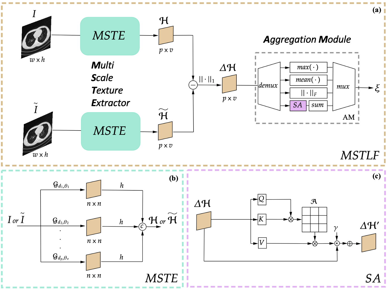
Figure 1: Overall framework of MSTLF. (a) MSTLF mainly includes two essential components, i.e., Multi-Scale Texture Extractor (MSTE) and Aggregation Module (AM). We denote the selection of the aggregation rule with the logic operators demux and mux. (b) MSTE module and (c) dynamic aggregation by Self-Attention mechanism (SA). First, MSTE extracts a textural representation from the GLCMs at different spatial and angular scales; second, AM combines the extracted representation into a scalar loss function.

2.1 Multi-Scale Texture Loss Function

Let’s assume that $\bm{I}\in\mathbb{R}^{h\times w}$ and $\tilde{\bm{I}}\in\mathbb{R}^{h\times w}$ are a real and an approximated image, i.e., an image that belongs to the domain of interest and an image generated by a GAN, respectively, where $h$ and $w$ represent their height and width. Following  Figure 1 (a), both $\bm{I}$ and $\tilde{\bm{I}}$ are passed to the MSTE module to extract a multiscale textural representation based on GLCMs, i.e., $\bm{\mathcal{H}}$ and $\bm{\mathcal{\tilde{H}}}$.

We now describe how to extract $\bm{\mathcal{H}}$ and $\bm{\mathcal{\tilde{H}}}$. For fixed spatial and angular offset denoted as $d$ and $\theta$, respectively, the GLCM is defined as a squared matrix $\bm{\mathcal{G}}_{d,\theta}\in\mathbb{R}^{n\times n}$, so that each element at coordinate $(i,j)$ lies in the range $[0,1]$. Each of its elements is computed as:

$$\bm{\mathcal{G}}_{d,\theta}(i,j)=\frac{g_{d,\theta}(i,j)}{\sum_{i=1}^{n}\sum_{j=1}^{n}g_{d,\theta}(i,j)}$$ (2)

where,

$$g_{d,\theta}(i,j)=\sum_{x=1}^{w}\sum_{y=1}^{h}\delta[\bm{I}(x,y)=i]\cdot\delta[\bm{I}(\tilde{x},\tilde{y})=j]$$ (3)

s.t.

$$\tilde{x}=x+d\cos\theta$$ (4)

$$\tilde{y}=y+d\sin\theta$$ (5)

where $\delta$ is the Kronecker delta function, and $g_{d,\theta}(i,j)$ counts the occurrences of pixel value $i$ and $j$.

Let $D=\{d_{1},d_{2},...,d_{p}\}$ and $\Theta=\{\theta_{1},\theta_{2},...,\theta_{v}\}$ be the sets of spatial and angular offsets, respectively. To obtain a multiscale texture representation ( Figure 1 (b)) we consider the cartesian product between $D$ and $\Theta$:

$$D\times\Theta=\{(d_{i},\theta_{j})|d_{i}\in D,\theta_{j}\in\Theta\},$$ (6)

Let’s now assume that $h$ is an operator extracting a texture descriptor from $\bm{\mathcal{G}}_{d,\theta}(i,j)$ (more details in section 2.2).
We compute a multi-scale texture representation $\bm{\mathcal{H}}\in\mathbb{R}^{p\times v}$ of $\bm{I}$ as:

$$\bm{\mathcal{H}}=\begin{bmatrix}h(\bm{\mathcal{G}}_{d_{1},\theta_{1}})&...&...&...&...\\ ...&...&...&...&...\\ ...&...&h(\bm{\mathcal{G}}_{d_{i},\theta_{j}})&...&...\\ ...&...&...&...&...\\ ...&...&...&...&h(\bm{\mathcal{G}}_{d_{p},\theta_{v}})\end{bmatrix}$$ (7)

Similarly, for $\bm{I}$ we compute $\bm{\mathcal{\tilde{H}}}\in\mathbb{R}^{p\times v}$ (it is enough to replace $\bm{I}$ with $\bm{\tilde{I}}$ in Eq. 3).
Going back to  Figure 1 (a), we then compute the error deviation $\bm{\Delta\mathcal{H}}\in\mathbb{R}^{p\times v}$ as:

$$\bm{\Delta\mathcal{H}}=||\bm{\mathcal{H}}-\bm{\mathcal{\tilde{H}}}||_{1}.$$ (8)

The aggregation module AM combines textural information into a scalar $\xi$:

$$\xi=AM(\bm{\Delta\mathcal{H}}).$$ (9)

We investigate two approaches for AM that we refer to as static and dynamic aggregation. In the first case, the aggregation is static because it is defined by mathematical operators performing the aggregation, as follows:

• Maximum: $\xi=max(\bm{\Delta\mathcal{H}})$, which leads the optimization to focus on the most discrepant texture descriptor.

• Average: $\xi=mean(\bm{\Delta\mathcal{H}})$, which leads the optimization to focus on the average discrepancy among texture descriptors.

• Frobenius norm: $\xi=||\bm{\Delta\mathcal{H}}||_{F}=\sqrt{Tr(\bm{\Delta\mathcal{H}}\cdot\bm{\Delta\mathcal{H}}^{H})}$, similar to the average but performing a non-linear aggregation. $Tr$ is the trace operator whilst $H$ denotes the Hermitian operator.

In the second case, the aggregation is dynamic since it enables the model to adaptively capture relationships between texture descriptors during the training of the model. Inspired by [59], this approach is implemented as a self-attention layer (Fig. 1 (c)): $\bm{\Delta\mathcal{H}}$ is passed through an attention layer which first applies $1\times 1$ convolutions to extract keys $\bm{\mathcal{K}}$, queries $\bm{\mathcal{Q}}$ and values $\bm{\mathcal{V}}$. Then, the aggregation is computed as:

$$\xi=<\mathbf{1}_{p\cdot v},vec(\bm{\Delta\mathcal{H}}^{{}^{\prime}})>$$ (10)

where,

$$\bm{\Delta\mathcal{H}}^{{}^{\prime}}=\gamma\bm{\mathcal{A}}\bm{\mathcal{V}}+\bm{\Delta\mathcal{H}}$$ (11)

s.t.

$$\bm{\mathcal{A}}=SoftMax(\bm{\mathcal{Q}}^{T}\bm{\mathcal{K}}).$$ (12)

$\bm{\Delta\mathcal{H}}^{{}^{\prime}}\in\mathbb{R}^{p\times v}$ is the output of the attention layer, $\mathbf{1}_{p\cdot v}$ is a vector of ones of size $p\cdot v$, $vec(\bm{\Delta\mathcal{H}}^{{}^{\prime}})$ is the vectorized error deviation, $<\cdot,\cdot>$ indicates the inner product, $\bm{\mathcal{A}}\in\mathbb{R}^{(p\cdot v)\times(p\cdot v)}$ denotes the attention map and $\gamma$ is a trainable scalar weight.

Without loss of generality, we extend the derivation of our method to the entire image batch of size $b$:

$$\bm{\Xi}=[\ \xi_{1},\xi_{2},...\xi_{b}]\ ^{T}$$ (13)

Then, the overall MSTLF is computed as:

$$\mathcal{L}_{txt}=mean(\bm{\Xi})=\frac{1}{b}<\mathbf{1}_{b},\bm{\Xi}>$$ (14)

where $\mathbf{1}_{b}$ is a vector of ones of size $b$.

2.2 Which texture descriptor?

The texture descriptor $h$, introduced in section 2.1, can be expressed in different forms and, here, we rely on well-established Haralick features ([10]), namely the contrast, homogeneity, correlation, and angular second momentum, which are presented in Table 1. Denoting as $f(i,j)$ the term that gives a specific Haralick feature, we have for $h$

$$h(\bm{\mathcal{G}}_{d,\theta})=\sum_{i=1}^{n}\sum_{j=1}^{n}f(i,j)\bm{\mathcal{G}}_{d,\theta}(i,j)$$ (15)

The same Table 1 reports the order of magnitude of $\Delta h$, i.e., the difference between LDCT and HDCT images captured by the Haralick feature $h$ computed from 10 patients (not included in the other stages of this work) belonging to Mayo Clinic LDCT-and-Projection Data ([37]), showing that contrast is the most sensitive to noise since it captures relative differences two orders of magnitude larger than the others. This could be expected as the contrast strictly depends on the noise in an image: indeed, the Contrast-to-Noise Ratio (CNR) of two regions $A$ and $B$ is equal to the absolute difference between their Signal-to-Noise Ratio SNR:

$$CNR_{AB}=\frac{|S_{A}-S_{B}|}{\sigma_{N}}=|SNR_{A}-SNR_{B}|$$ (16)

where $S_{A}$ and $S_{B}$ are the signals from image region $A$ and $B$, and $\sigma_{N}$ is the standard deviation of the noise. Hence, if we assume that the noise corruption over the entire image is approximately uniform, an increase in noise corresponds to a decrease in contrast.

$\bm{h}$	$\bm{f(i,j)}$	Magnitude of $\Delta h$
Contrast	$(i-j)^{2}$	$\sim 10^{2}$
Homogeneity	$\frac{1}{1-(i-j)^{2}}$	$\sim 10^{-2}$
Correlation	$\frac{(i-\mu_{i})(j-\mu_{j})}{\sqrt{\sigma_{i}^{2}\sigma_{j}^{2}}}$	$\sim 10^{-3}$
Angular second moment	$\bm{\mathcal{G}}_{d,\theta}(i,j)$	$\sim 10^{-2}$

Table 1: Definition of 4 well-established Haralick features and order of magnitude of the difference captured ($\Delta h$) between LDCT images and HDCT images computed from 10 patients (not included in the other stages of this work) belonging to Mayo Clinic LDCT-and-Projection Data ([37]). The larger the value of $\Delta h$ the higher the sensitivity to noise.

2.3 How to make the GLCM differentiable

Differentiability is a key feature of any deep-learning framework. Whenever a new loss function or a regularization term is introduced, its implementation must be differentiable, i.e., it must be compatible with gradient-based optimization, enabling the backpropagation of the gradient throughout the entire model. However, the GLCM is not differentiable by its very nature, since it is essentially a histogramming operation and hence it does not align with gradient-based optimization frameworks. For this reason, we propose a soft approximation of the GLCM which makes it a continuous and differentiable function.

To implement a differentiable GLCM, we employ a Gaussian soft assignment function for each pixel value to a set of predefined bins:

$$a_{k}(\bm{I}(x,y))=e^{-\frac{(\bm{I}(x,y)-b_{k})^{2}}{2\sigma^{2}}}$$ (17)

where $\bm{I}(x,y)$ is the pixel value in position $(x,y)$, $b_{k}$ is the $k^{th}$ bin value and $\sigma$ is a hyperparameter denoting the standard deviation of the Gaussian assignment function. The latter is chosen due to its smooth bell-shaped curve, which helps in assigning weights to neighboring bins, ensuring a soft transition between them. Furthermore, $\sigma$ controls the spread of the Gaussian: a lower $\sigma$ creates sharper assignments (closer to hard binning), while a higher $\sigma$ makes it softer, spreading the value across multiple bins. In our experiments, $\sigma$ is set to 0.5 which results in a negligible error in the calculation of the soft GLCM of the order of $\sim 10^{-11}$. To ensure that the weights sum up to one, preserving the nature of probability, we normalize the soft assignment for each pixel with respect to all bins:

$$a^{\prime}(\bm{I}(x,y))=\frac{a_{k}}{\sum_{k=1}^{n}a_{k}(\bm{I}(x,y))}$$ (18)

Given two images (original $\bm{I}$ and the corresponding spatially shifted $\bm{I_{d,\theta}}$ by the specified distance $d$ and angle $\theta$) and their soft assignments $a^{\prime}(\bm{I}(x,y))$, the soft GLCM is obtained using the outer product:

$$\bm{\mathcal{G}}_{d,\theta}^{i,j}=\sum_{x=1}^{h}\sum_{y=1}^{w}a^{\prime}(\bm{I}(x,y))\times a^{\prime}(\bm{I_{s}}(x,y))$$ (19)

where the outer product $\times$ ensures that all possible combinations of pixel intensity relationships are considered, providing a comprehensive texture descriptor. It is worth noting that the entire process consists of differentiable operations, from Gaussian soft assignment to normalization and the outer product followed by summation, making the soft GLCM a differentiable function with respect to the input image $\bm{I}$. Furthermore, this method generalizes to any number of gray levels and can handle images of any bit depth without binning or down-scaling.

2.3.1 Computational Cost Analysis

Given that the Soft GLCM is a differentiable alternative to the traditional GLCM, it is crucial to analyze and compare the computational costs of these two methods.

The computational process of the traditional GLCM involves iterating through each pixel in the image and updating a co-occurrence count in the GLCM matrix. If the total number of pixels in the image is denoted as $N=h\cdot w$ and the size of the GLCM matrix as $n\times n$, the computation for each pixel pair is a constant time operation, $\mathcal{O}(1)$. Thus, the overall computational complexity of the traditional GLCM method scales linearly with the number of pixels, resulting in a complexity of $\mathcal{O}(N)$.

In contrast, the Soft GLCM incorporates a Gaussian soft assignment for each pixel value against a set of predefined bins, followed by the construction of the GLCM using these soft assignments. This procedure involves a two-fold computational process for each pixel: the soft assignment and the GLCM construction. In the soft assignment, each pixel value is subjected to a Gaussian computation against each bin, followed by a normalization step, incurring a complexity of $\mathcal{O}(n)$ per pixel. The construction of the GLCM from these soft assignments involves calculating the outer product of the soft assignment vectors of each pixel pair, resulting in a computational complexity of $\mathcal{O}(n^{2})$ for each pixel. Aggregating these computations, the Soft GLCM presents a total computational complexity of $\mathcal{O}(N\cdot n^{2})$, which is quadratic in the number of gray levels and linear in the number of pixels. We note that for images with high resolution or high bit depth, the Soft GLCM becomes significantly more computationally expensive compared to the traditional GLCM, but comes with the benefit of differentiability, which is crucial for gradient-based optimization in deep learning frameworks. This allows its integration into the deep learning framework, which enables leveraging parallel GPU tensor computations and batch-level processing, thus mitigating the computational overhead to a large extent.

3 Experimental Configuration

This section describes the deep models considered, the data used, the implementation details, and the evaluation metrics. Let us remember that $\bm{x}\in X$ is a LDCT image, whilst $\bm{y}\in Y$ is an HDCT image. To show the effectiveness of our method we validate our approach on three of the most widely used generative architectures ([40]) in the image translation landscape: Pix2Pix ([19]), CycleGAN ([61]), and UNIT ([32]). The interested reader may refer to section 1 in the supplementary material for a detailed description of the three architectures.

	Experiment	Loss function
Competitors	Baseline	$\mathcal{L}$
	VGG-16	$\mathcal{L}+\mathcal{L}_{VGG}$
	AE-CT	$\mathcal{L}+\mathcal{L}_{AE}$
	SSIM-L	$\mathcal{L}+\mathcal{L}_{ssim}$
	EDGE	$\mathcal{L}+\mathcal{L}_{\nabla^{2}}$
Our approach	MSTLF-max	$\mathcal{L}+\mathcal{L}_{txt}^{max}$
	MSTLF-average	$\mathcal{L}+\mathcal{L}_{txt}^{avg}$
	MSTLF-Frobenius	$\mathcal{L}+\mathcal{L}_{txt}^{Frob}$
	MSTLF-attention	$\mathcal{L}+\mathcal{L}_{txt}^{att}$

Table 2: List of the proposed loss function configurations. For Pix2Pix, CycleGAN, and UNIT, the baseline loss function $\mathcal{L}$ is implemented as reported in section 1 in the supplementary material.

3.1 Loss functions

We design experiments such that variations in performance are only attributed to variations in the loss function used. As shown in Table 2, we considered nine different configurations, where each configuration distinguishes from the others by adding a loss function term to the baseline loss function $\mathcal{L}$. The first five configurations are competitors introduced in section 1, whilst the remaining four are different implementations of MSTLF that vary in the type of aggregation used to combine the texture descriptors.

For each model architecture, the first configuration is the baseline implemented in its original version reported in the supplementary material. The second is the perceptual loss function $\mathcal{L}_{VGG-16}$ that is computed starting from the deep features extracted from the VGG-16 network ([46]), pre-trained on ImageNet ([43]). This loss term, originally introduced in ([15]), stems from observing that the similarity of features obtained from CNNs may indicate the level of semantic similarity between the images they come from providing an additional informative contribution compared to the traditional pixel-wise term ([39]). Given a generic image $\bm{I}$ and its approximation $\bm{\tilde{I}}$, $\mathcal{L}_{VGG}$ is computed as ([21]):

$$\mathcal{L}_{VGG}=\frac{1}{W\cdot H\cdot D}\sum_{i=1}^{5}||\bm{\phi_{i}}(\bm{\tilde{I}})-\bm{\phi_{i}}(\bm{I})||_{2}^{2}$$ (20)

where $\bm{\phi_{i}}$ is the $i^{th}$ pooling layer of the VGG-16 and $W$, $H$, $D$ are its width, height, and depth, respectively.

As mentioned in section 1, deep feature extractors, pre-trained on ImageNet, can produce sub-optimal features when used in domains other than the natural image domain ([35]). For this reason, we implement a deep feature extractor trained on CT images ([16, 27, 17]). We adopt the self-supervised approach proposed by ([27]) that trains an auto-encoder network to extract an encoding from the input CT image that is then used to reconstruct an output CT image as close as possible to the input. We trained the auto-encoder with 8 patients (not included in the other stages of this work) for a total of 2824 images; among them, 4 belong to the Mayo Clinic LDCT-and-Projection Data ([37]) and the remaining 4 belong to the Lung Image Database Consortium and Image Database Resource Initiative (LIDC-IDRI) ([2]). By utilizing data from two distinct datasets, we aimed to enhance the heterogeneity of the learned data distribution. We then use the encoded representation to compute the perceptual loss $\mathcal{L}_{AE}$ (third row in Table 2):

$$\mathcal{L}_{AE}=\frac{||\bm{e}(\bm{\tilde{I}})-\bm{e}(\bm{I})||_{2}^{2}}{W\cdot H\cdot D}$$ (21)

where $\bm{e}$ is the encoded representation and $W$, $H$, $D$ are its width, height, and depth, respectively.

The fourth loss function is based on structural similarity ([51]). $\mathcal{L}_{ssim}$, proposed as a more sophisticated and robust distance than the traditional $L_{1}$ and $L_{2}$ distances ([30, 29, 57]), is computed as:

$$\mathcal{L}_{ssim}=1-SSIM(\bm{\tilde{I}},\bm{I})$$ (22)

where $SSIM$ is the structural similarity index, described in section 3.3.

To overcome the limitations posed by $L_{1}$ and $L_{2}$ distances, some authors propose the use of the Charbonnier distance which is a smooth approximation of the Huber loss ([8, 14, 28, 22]) that is quadratic for small variations and approximates the $L_{1}$ distance for large variations.

As fifth competitor, named edge loss, we use the Charbonnier distance $\mathcal{L}_{\nabla^{2}}$ ([26, 58]), which minimizes the distance between Laplacians instead of pixel-intensities. It is given by:

$$\mathcal{L}_{\nabla^{2}}=\sqrt{||\nabla^{2}(\bm{\tilde{I}})-\nabla^{2}(\bm{I})||^{2}+\epsilon^{2}}$$ (23)

where $\nabla^{2}$ denotes the Laplacian operator and $\epsilon^{2}$ is a constant empirically set to $10^{-3}$. It is also interesting to note that $\mathcal{L}_{\nabla^{2}}$ catches a gradient-based quantity that maps edge information in the image, i.e., a feature different from the textural data we represent in our approach.

The last four loss functions shown in Table 2 are $\mathcal{L}_{txt}^{max}$, $\mathcal{L}_{txt}^{avg}$,$\mathcal{L}_{txt}^{Frob}$,$\mathcal{L}_{txt}^{att}$ which differ in the type of aggregation used to combine texture descriptors. As mentioned in section 2.1, we have four approaches in the AM: three are static (maximum, average and Frobenius) and they are denoted as $\mathcal{L}_{txt}^{max}$, $\mathcal{L}_{txt}^{avg}$, $\mathcal{L}_{txt}^{Frob}$, respectively. The fourth, named $\mathcal{L}_{txt}^{att}$, is dynamic and it makes use of an attention mechanism. Before concluding this subsection, we detail how we apply MSTLF for each of the three GANs, graphically presented in Figure 2.

Without loss of generality, let $\mathcal{L}_{txt}$ be a generic MSTLF. In Pix2Pix, we apply MSTLF between a generated image $\bm{\hat{y}}=G(\bm{x},\bm{z})$ and its reference ground truth $y$, i.e., $\mathcal{L}_{txt}(\bm{\hat{y}},\bm{y})$ (Figure 2 (a)). In CycleGAN, we apply MSTLF to enforce the cycle consistency constraint between an image and its reconstruction in both the domains, i.e., $\mathcal{L}_{txt}(\bm{\tilde{x}},\bm{x})$, $\mathcal{L}_{txt}(\bm{\tilde{y}},\bm{y})$ where $\bm{\tilde{x}}=F(G(\bm{x}))$ and $\bm{\tilde{y}}=G(F(\bm{y}))$ are reconstructed images in the source domain $X$ and the target domain $Y$, respectively (Figure 2 (b)). In UNIT, MSTLF is applied as, $\mathcal{L}_{txt}(\bm{\hat{x}},\bm{x})$, $\mathcal{L}_{txt}(\bm{\hat{y}},\bm{y})$ where $\bm{\hat{x}}=G_{X}(\bm{\hat{z}_{X}})$ and $\bm{\hat{y}}=G_{Y}(\bm{\hat{z}_{Y}})$ (Figure 2 (c)).

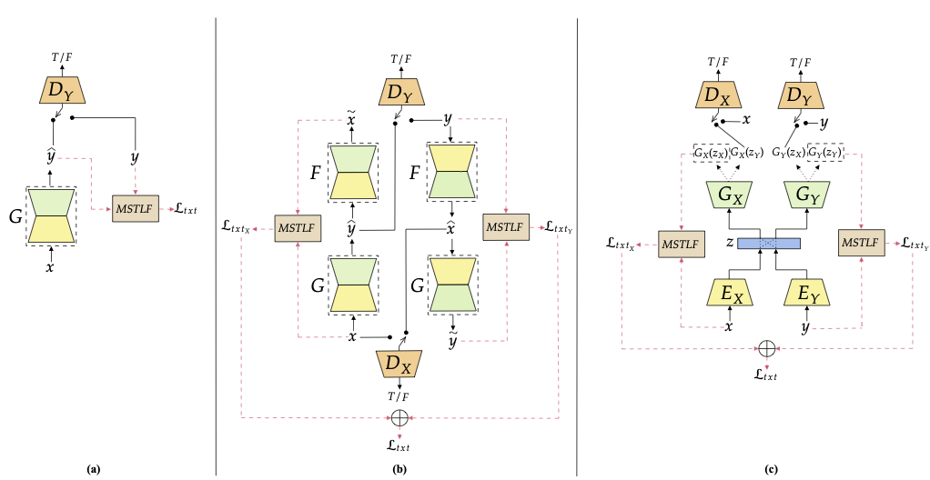
Figure 2: GAN architectures showing how MSTLF is applied. (a) Pix2Pix (b) CycleGAN (c) UNIT. The red dashed arrows denote the loss function computation. In UNIT, we use black dotted arrows to distinguish between different generation paths. $G$ and $F$ denotes generator networks, $D_{X}$ and $D_{Y}$ indicates discriminator networks, whilst $E_{X}$ and $E_{Y}$ are encoders and $G_{X}$ and $G_{Y}$ are decoders.

3.2 Materials

We use three public datasets that contain paired and unpaired images. The first is the Mayo Clinic LDCT-and-Projection Data ([37]) which includes thoracic and abdominal HDCT and corresponding LDCT data simulated by a quarter dose protocol. We took 17 patients; among them, 10 are those used in the Mayo Clinic for the 2016 NIH-AAPM-Mayo Clinic Low Dose CT Grand Challenge and 9 out of 10, corresponding to 5376 CT slices, are used for training as other works on LDCT denoising did ([31, 47, 33, 30]). The test set, denoted as Dataset A in the following, contains 2994 slices from 8 patients: 1 patient from the aforementioned 10, plus other 7 patients randomly selected from ([37]) to make the evaluation more robust.. The evaluation on the Mayo Clinic LDCT-and-Projection Data permits us to compute paired metrics reported in section 3.3, but it could be limited by the fact that LDCT images are simulated. To overcome this limitation we consider two real LDCT datasets that, straightforwardly, do not contain HDCT images. They are the Lung Image Database Consortium and Image Database Resource Initiative (LIDC/IDRI) ([2]) and the ELCAP Public Image Database ([50]), named Dataset B and Dataset C hereinafter. From the former, we included 8 patients for a total of 1831 LDCT images, whilst from the latter we used the scans from 50 patients for a total of 12360 LDCT images.

3.3 Performance metrics

In ([11]), they brought out that paired and unpaired metrics generally lead to different but complementary results, that is, they measure image quality from different perspectives. Here we used five image quality assessment metrics: Mean Square Error (MSE), Peak-Signal-to-Noise Ratio (PSNR), Structural Similarity Index (SSIM), Natural Image Quality Evaluator (NIQE), and Perception Based Image QUality Evaluator (PIQUE). The first three metrics perform a paired evaluation, i.e., they require pairs of images to be computed, whilst the last two relax this constraint performing a no-reference evaluation ([11]). Both PSNR and MSE serve as error-based metrics, appropriate for quantifying the degree of image distortion without necessarily implying visually favorable outcomes. While SSIM has been introduced as a more sophisticated metric compared to the aforementioned two, it is better suited for measuring distortion rather than perception ([5, 48]). Oppositely, NIQE and PIQUE are blind image quality assessment scores that only make use of measurable deviations measuring the perception ([36, 49]).

MSE

MSE computes the absolute difference between intensities in pixels of the denoised and reference image:

$$MSE(\bm{\hat{y}},\bm{y})=\frac{1}{mn}\sum_{i=0}^{m-1}\sum_{j=0}^{n-1}\left[\bm{\hat{y}}(i,j)-\bm{y}(i,j)\right]^{2}$$ (24)

where $(i,j)$ is the pixel coordinates, and $m$, $n$ are the numbers of columns and rows, respectively. It ranges from 0 to $+\infty$. A lower MSE indicates a better match between the denoised and the reference image.

PSNR

PSNR compares the maximum intensity in the image ($MAX_{\bm{\hat{y}}}$) with the error between $\bm{\hat{y}}$ and $\bm{y}$ given by the MSE:

$$PSNR(\bm{\hat{y}},\bm{y})=10\times log_{10}\left(\frac{MAX_{\bm{\hat{y}}}^{2}}{MSE(\bm{\hat{y}},\bm{y})}\right).$$ (25)

It ranges from 0 to $+\infty$ and it is expressed in decibels. Higher PSNR values indicate better quality, while lower values may suggest more noticeable distortions or errors in the denoised image.

SSIM

SSIM computes the local similarity between two images as a function of luminance, contrast, and structure ([51]):

$$SSIM(\bm{\hat{y}},\bm{y})=\frac{(2\mu_{\bm{\hat{y}}}\mu_{\bm{y}}+C_{1})(2\sigma_{\bm{\hat{y}}\bm{y}}+C_{2})}{(\mu_{\bm{\hat{y}}}^{2}+\mu_{\bm{y}}^{2}+C_{1})(\sigma_{\bm{\hat{y}}}^{2}+\sigma_{\bm{y}}^{2}+C_{2})}$$ (26)

where $\mu_{\bm{\hat{y}}}$, $\mu_{\bm{y}}$ are mean intensities of pixels in $\bm{\hat{y}}$ and $\bm{y}$, respectively; similarly $\sigma_{\bm{\hat{y}}}^{2}$ and $\sigma_{\bm{y}}^{2}$ are the variances, $\sigma_{\bm{\hat{y}}\bm{y}}$ is the covariance whilst $C_{1}$ and $C_{2}$ are constant values to avoid numerical instabilities. It lies in $[0,1]$ with values closer to 1 indicating better image quality.

NIQE

NIQE uses measurable deviations from statistical regularities observed in a corpus of natural images to quantify image perception, fitting a multivariate Gaussian model ([36]):

$$\begin{split}NIQE(\nu_{1},\nu_{\bm{\hat{y}}},\Sigma_{1},\Sigma_{\bm{\hat{y}}})\\ =\left(\sqrt{(\nu_{1}-\nu_{\bm{\hat{y}}})^{T}\left(\frac{\Sigma_{1}+\Sigma_{\bm{\hat{y}}}}{2}\right)^{-1}(\nu_{1}-\nu_{\bm{\hat{y}}})}\right)\cdot 100\end{split}$$ (27)

where $\nu_{1}$, $\Sigma_{1}$, $\nu_{\bm{\hat{y}}}$, $\Sigma_{\bm{\hat{y}}}$ are the mean vectors and covariance matrices of the natural multivariate Gaussian model and the denoised image’s multivariate Gaussian model, respectively. It lies in $[0,100]$, with values closer to $0$ indicating better image quality.

PIQUE

PIQUE measures perception in a denoised image exploiting local characteristics extracted from $16\times 16$ non-overlapping blocks ([49]):

$$\begin{split}PIQUE(\bm{\hat{y}})=\left(\frac{\left(\sum_{k=1}^{N_{SA}}D_{sk}\right)+C_{1}}{N_{SA}+C_{1}}\right)\cdot 100\end{split}$$ (28)

where $D_{sk}$ captures the distortion of each image block, $N_{SA}$ is the number of distorted blocks and $C_{1}$ is a constant to prevent numerical instability. It lies in $[0,100]$, with values closer to $0$ indicating better image quality.

3.4 Implementation Details

We preprocess all the images as follows: first, we convert all the raw DICOM files to Hounsfield Unit (HU), second, we select a display window centered in -500 HU with a width of 1400 HU, emphasizing lung tissue, third, we normalize all the images in the range [-1, 1] and resized to $256\times 256$. The training dataset is paired, as mentioned in section 3.2: hence, we trained the Pix2Pix in a paired manner, while we trained CycleGAN and UNIT in an unpaired manner by scrambling all the training images to avoid paired correspondence between HDCT and LDCT images for each training batch. We trained all the models for 50 epochs, with a batch size of 16. All the networks are initialized with normal initialization and optimized by Adam optimizer ([24]) with default learning rates of $2\cdot 10^{-4}$ for Pix2Pix and CycleGAN and $10^{-4}$ for UNIT. We set the weights of the baseline loss functions according to the original implementations, as described in the supplementary material. The weights of perceptual losses, edge loss, and SSIM loss were set to $\lambda_{VGG}=0.1$, $\lambda_{AE-CT}=10^{3}$, $\lambda_{EDGE}=10$, $\lambda_{SSIM}=1$, respectively. The weights of MSTLFs were set to $\lambda_{txt}^{max}=\lambda_{txt}^{avg}=\lambda_{txt}^{Frob}=10^{-3}$, $\lambda_{txt}^{att}=1$. The latter refers to MSTLF-attention and it was set to 1, as the self-attention layer incorporates its normalization and does not require external scaling. Our MSTLF used a set of spatial offsets $D=\{1,3,5,7\}$ and a set of angular offsets $\Theta=\{0^{\circ},45^{\circ},90^{\circ},135^{\circ}\}$. All the models are parallelized on 4 NVIDIA Tesla A100, allowing for faster training time. We repeat each experiment three times to make the results more robust, mitigating the intrinsic variability that characterizes GANs’ training. We assess the average statistical significance of each experiment through the Wilcoxon Signed rank Test with $p<0.05$.

4 Results and Discussion

This section performs an in-depth analysis to assess the effects of our MSTLF on LDCT denoising, providing both quantitative evaluations and visual examples.

  Experiment Dataset A PSNR $\uparrow$ MSE $\uparrow$ SSIM $\uparrow$ NIQE $\downarrow$ PIQUE $\downarrow$   LDCT - 17.7322 $2.25\cdot 10^{-3}$ 0.5832 17.0272 23.5495 Pix2Pix Baseline 21.3344 $10.50\cdot 10^{-3}$ 0.7335 6.5263 8.6017 VGG-16 21.3481 $10.41\cdot 10^{-3}$ 0.7293 6.5673 8.7114 AE-CT 21.3422 $10.55\cdot 10^{-3}$ 0.7349 6.1640 8.9156 SSIM-L 21.4011 $10.37\cdot 10^{-3}$ $\textbf{0.7426}^{**}$ 6.0690 8.2995 EDGE 21.0620 $10.63\cdot 10^{-3}$ 0.7196 6.4413 8.7461 MSTLF-max 21.3234 $10.50\cdot 10^{-3}$ 0.7284 6.5024 8.7950 MSTLF-average $\textbf{21.4497}^{**}$ $\mathbf{{10.32}\cdot 10^{-3**}}$ 0.7379 6.2366 8.5473 MSTLF-Frobenius 21.3661 $10.42\cdot 10^{-3}$ 0.7347 6.0670 8.8096 MSTLF-attention 20.7495 $11.62\cdot 10^{-3}$ 0.7103 $\textbf{5.1934}^{**}$ $\textbf{7.3575}^{**}$ CycleGAN Baseline 20.8588 $10.15\cdot 10^{-3}$ 0.6935 9.6203 12.6893 VGG-16 20.7759 $10.17\cdot 10^{-3}$ 0.6997 10.1728 13.3256 AE-CT 21.2143 $9.69\cdot 10^{-3}$ 0.7092 8.0317 8.7166 SSIM-L 20.6699 $10.50\cdot 10^{-3}$ 0.6919 10.2733 13.0187 EDGE 20.5538 $10.84\cdot 10^{-3}$ 0.6928 10.7092 13.5882 MSTLF-max 20.9735 $9.70\cdot 10^{-3}$ 0.7013 9.2843 11.9323 MSTLF-average $\textbf{21.2529}^{**}$ $\mathbf{{9.32}\cdot 10^{-3**}}$ $\textbf{0.7114}^{**}$ 8.6642 10.9737 MSTLF-Frobenius 21.1883 $9.54\cdot 10^{-3}$ 0.7108 8.5100 11.1255 MSTLF-attention 20.6741 $9.89\cdot 10^{-3}$ 0.7058 $\textbf{5.3209}^{**}$ $\textbf{5.4432}^{**}$ UNIT Baseline 21.4333 $8.85\cdot 10^{-3}$ 0.7203 6.4581 8.3179 VGG-16 21.4207 $8.54\cdot 10^{-3}$ 0.7296 6.5030 7.7908 AE-CT 22.0836 $7.68\cdot 10^{-3}$ 0.7450 7.2524 7.6388 SSIM-L 22.1704 $7.64\cdot 10^{-3}$ 0.7465 7.4184 7.5623 EDGE 21.9671 $7.83\cdot 10^{-3}$ 0.7434 6.6897 $\textbf{7.2272}^{**}$ MSTLF-max $\textbf{22.2671}^{**}$ $\mathbf{7.32\cdot 10^{-3**}}$ $\textbf{0.7480}^{**}$ 6.8441 7.5657 MSTLF-average 22.0836 $7.70\cdot 10^{-3}$ 0.7429 6.7520 7.8877 MSTLF-Frobenius 22.1601 $7.41\cdot 10^{-3}$ 0.7458 7.1659 7.7813 MSTLF-attention 22.1270 $7.39\cdot 10^{-3}$ 0.7426 $\textbf{6.0238}^{**}$ 7.4101  

Table 3: Quantitative comparison of different loss function configurations on the simulated test set. The numerical values are the average values over three repetitions of each experiment. Bold text and two asterisks denote best results per metric and per architecture satisfying $p<0.05$; bold text and a single asterisk highlight the best results in a section with $p\geq 0.05$ among themselves, while satisfying $p<0.05$ wrt to the other experiments.

  Experiment Dataset B Dataset C NIQE $\downarrow$ PIQUE $\downarrow$ NIQE $\downarrow$ PIQUE $\downarrow$   LDCT - 13.6189 20.3687 11.8081 15.1818 Pix2Pix Baseline 5.5597 8.9952 5.4423 6.9620 VGG-16 5.5726 8.8453 5.4671 6.8522 AE-CT 5.1338 8.4187 5.0586 6.4835 SSIM-L 5.1439 8.3272 5.1091 $\textbf{6.2623}^{*}$ EDGE 5.5052 9.5456 5.6078 7.4611 MSTLF-max 5.5234 9.0999 5.4585 7.061 MSTLF-average 5.2658 8.7173 5.2390 6.6374 MSTLF-Frobenius 5.1832 8.5485 5.1944 6.7230 MSTLF-attention $\textbf{4.8728}^{**}$ $\textbf{7.3443}^{**}$ $\textbf{4.8634}^{**}$ $\textbf{6.2841}^{*}$ CycleGAN Baseline 8.6468 12.6395 8.3811 10.5286 VGG-16 8.3012 10.9972 8.1010 9.0185 AE-CT 7.1581 7.3931 6.9573 6.5963 SSIM-L 8.9653 12.2665 8.7280 10.2850 EDGE 8.9325 12.4375 8.6059 10.3436 MSTLF-max 8.3655 11.7319 8.1205 9.9322 MSTLF-average 7.9853 11.6693 7.8831 9.9328 MSTLF-Frobenius 7.5627 10.8876 7.4276 9.0732 MSTLF-attention $\textbf{5.1713}^{**}$ $\textbf{6.2002}^{**}$ $\textbf{5.1967}^{**}$ $\textbf{5.7071}^{**}$ UNIT Baseline 5.9253 9.0455 5.9474 7.4220 VGG-16 5.9518 9.0618 5.9586 7.4170 AE-CT 6.7394 8.8963 6.6581 7.1964 SSIM-L 7.0960 8.5735 7.0274 6.9753 EDGE 6.4342 $\textbf{7.9593}^{**}$ 6.3607 $\textbf{6.5470}^{**}$ MSTLF-max 6.5491 8.4952 6.5070 6.8747 MSTLF-average 6.4214 9.1836 6.4317 7.4392 MSTLF-Frobenius 6.6947 8.9574 6.6231 7.2449 MSTLF-attention $\textbf{5.5228}^{**}$ 8.5232 $\textbf{5.5433}^{**}$ 7.0860  

Table 4: Quantitative comparison of different loss function configurations on the real test sets. The numerical values are the average values over three repetitions of each experiment. Bold text and two asterisks denote best results per metric and per architecture satisfying $p<0.05$; bold text and a single asterisk highlight the best results in a section with $p\geq 0.05$ among themselves, while satisfying $p<0.05$ wrt to the other experiments.

Table 3 and Table 4 present the results of different experiments on simulated LDCT data (Dataset A), and real LDCT data (Dataset B and C), respectively. The two tables share the same structure: as a reference, the first row shows the values of the metrics computed on the LDCT images, which are used hereinafter to evaluate the relative improvement in image quality. The following rows are grouped in sections given the GAN backbone. For each section, there are nine experiments corresponding to the loss functions presented in section 3.1 and summarized in Table 2. In each section, we employ bold text and two asterisks to emphasize the best results per metric that exhibit statistically significant differences from the others. Additionally, we use bold text and a single asterisk to highlight the best results in a section that does not show statistically significant differences among themselves, while still satisfying $p<0.05$ compared to the other experiments.

Both Table 3 and 4 show that the proposed MSTLF approach performs better than the other loss functions on all the architectures in most of the cases: indeed, MSTLF has the largest number of bold values denoting the best results per metric and per architecture. For each GAN backbone, the Wilcoxon Signed rank Test shows that these best results are always statistically different (except for one case in Table 4) from the others. This finding is also confirmed when performing the same test on a per-patient basis, as shown in section 5 of the supplementary.

In Pix2Pix, MSTLF-average outperforms the other loss function configurations in terms of PSNR and MSE, while SSIM-L reaches the highest SSIM score, which is expected since SSIM-L is meant to maximize the SSIM. MSTLF-attention achieves the best result in NIQE and PIQUE on Dataset A, B, and C, proving to be effective on both simulated LDCT data and real LDCT data.

Turning our attention to the results attained using the CycleGAN, the results are consistent with those of Pix2Pix: MSTLF-average outperforms the other loss function configurations in all paired metrics while MSTLF-attention reaches the best performance in terms of unpaired metrics (NIQE and PIQUE) on all the datasets.

In UNIT, MSTLF-max is the best configuration focusing on paired metrics, while MSTLF-attention stands out in NIQE, as in Pix2Pix and CycleGAN. The best PIQUE instead is achieved by EDGE which, however, does not excel in any other metrics or architectures. On the contrary, MSTLF shows consistency of results on most metrics regardless of the architecture, showcasing a higher degree of agnosticism compared to other loss functions. We further observe that configurations that perform a static aggregation, i.e., MSTLF-max, MSTLF-average, MSTLF-Frobenius, favor paired metrics, whilst MSTLF-attention, performing dynamic aggregation, favors unpaired metrics.

Figure 3 shows an example of denoised images on Dataset A using the CycleGAN backbone. In panel (a) we report the HDCT and LDCT images followed by synthetic images provided by the nine experiments, whilst panel (b) shows the gradient of these images, to highlight noise in the image. For the sake of visualization, panel (c) shows the zoomed Regions Of Interest (ROIs) identified by the red boxes in the gradient images, which contain areas inside and outside the lung regions, thus including different tissues and anatomical structures. It is worth noting that MSTLF-attention produced the image with the lowest gradient that, in turn, corresponds to the lowest level of noise while preserving the lung boundaries (MSTLF-attention in Figure 3 (c)). Section 2 in the supplementary material completes the visual examples showing the results for the other two datasets and GAN backbones.

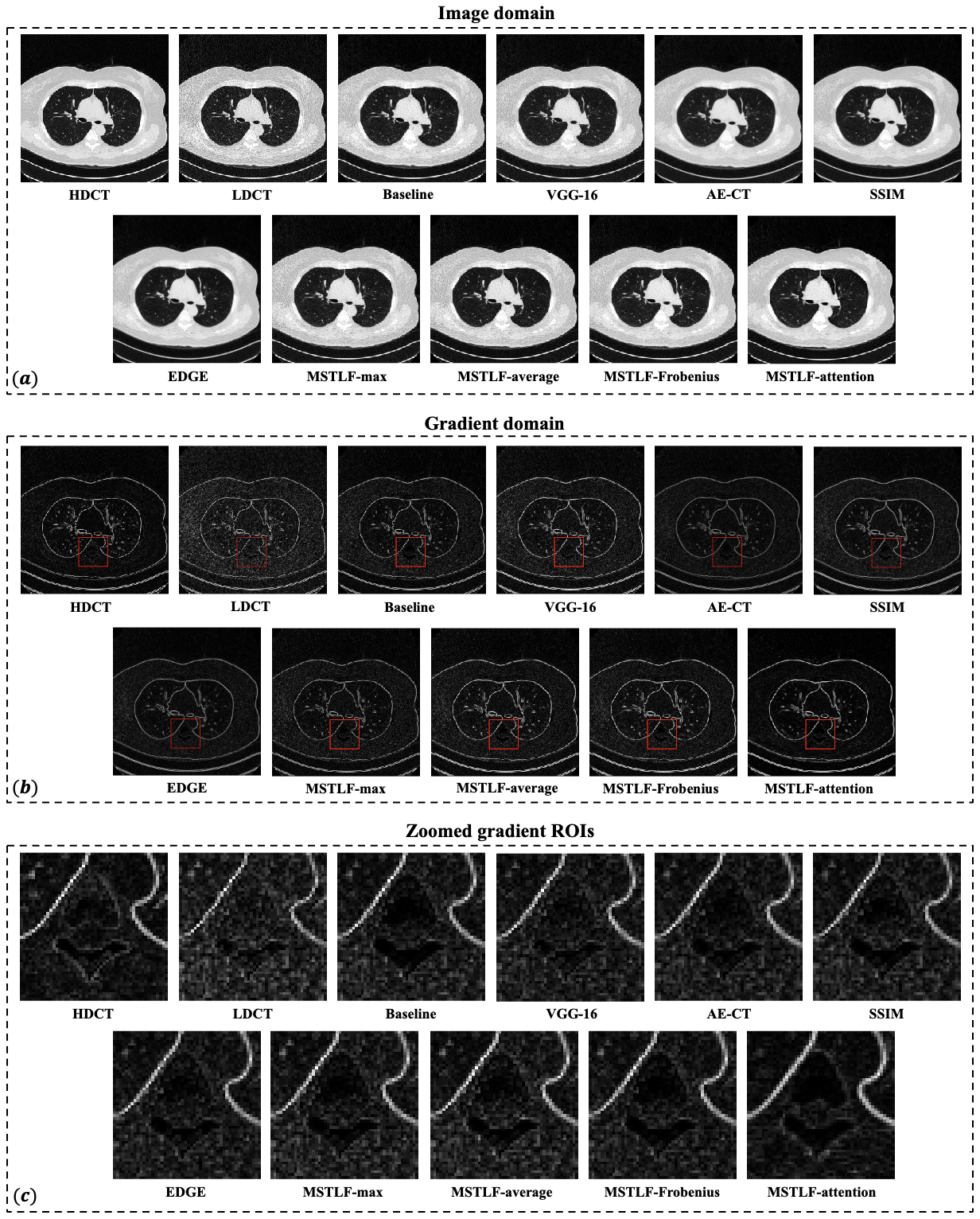
Figure 3: Visual comparison of denoised CT slices from the Mayo simulated data (Dataset A). We show all loss function configurations for CycleGAN (see supplementary for the remaining figures relative to CycleGAN, Pix2Pix and UNIT). The images are shown both in the image domain (panel (a) using a display window in [-1200, 200] HU), and the gradient domain (panel (b)). The zoomed ROI in panel (c) highlights denoising in the gradient domain.

4.1 The Perception-Distortion Trade-Off

[5] demonstrated that there exists a trade-off between perception and distortion when dealing with image restoration algorithms, that is, a low average distortion not necessarily implies a good perceptual quality and achieving both is an open challenge. From this consideration, we now look at our results from a perception-distortion perspective; as reported in section 3.3, perception is measured by NIQE and PIQUE, whereas distortion is measured by the MSE. Accordingly we represent each experiment by a point in the two perception-distortion planes (panels (a) and (b) of Figure 4). Then, we assess the trade-off between perception and distortion by ranking the experiments based on their proximity to the origin, as the point $(0,0)$ is the ideal one (Table 5). We find that MSTLF-attention is the one that reaches the best trade-off between perception and distortion, demonstrating consistent performance across different architectures. This outcome further supports the agnostic nature of our approach with respect to the GAN architecture.

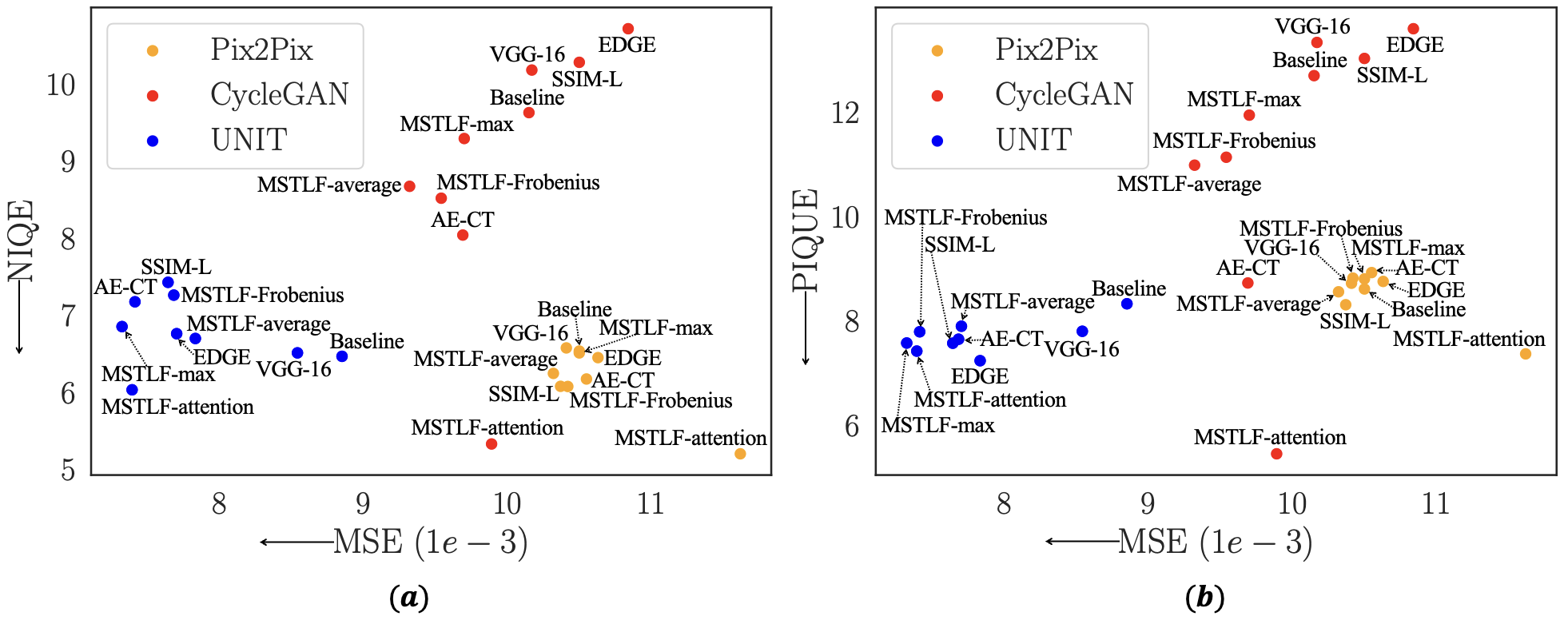
Figure 4: Perception-distortion evaluation of denoising algorithms. We plot the 9 experiments detailed in  Table 3.1 on the perception distortion plane. The color legend groups the experiments based on the GAN architecture. Distortion is measured by MSE in both panels, whilst perception is measured by NIQE and PIQUE in panel (a) and panel (b), respectively.

  Experiment NIQE vs MSE ranking PIQUE vs MSE ranking Pix2Pix CycleGAN UNIT Global Pix2Pix CycleGAN UNIT Global   Baseline 8 6 2 45 4 6 9 50 VGG-16 9 7 3 49 5 8 7 50 AE-CT 4 2 8 26 9 2 5 36 SSIM-L 3 8 9 31 2 7 3 36 EDGE 6 9 4 35 6 9 1 44 MSTLF-max 7 5 6 49 7 5 4 47 MSTLF-average 5 4 5 44 3 3 8 44 MSTLF-Frobenius 2 3 7 42 8 4 6 49 MSTLF-attention 1 1 1 6 1 1 1 8  

Table 5: Distance ranking in the perception-distortion plane.

4.2 Template Matching Analysis

To gain more insight into the denoising performance, we perform an analysis that quantifies the LDCT noise pattern still present in the corresponding denoised version. To this aim, let us remember that $\bm{x}$ is a LDCT image resized to $256\times 256$ (see section 3.4), now belonging to a set of $d$ test images. Furthermore, $\bm{T}\in\bm{x}$ denotes a template of size $t\times t$ (with $t=32$) extracted from $\bm{x}$ at a given location. To quantify the aforementioned noise pattern we proceed as follows. First, we compute the maximum template matching between $\bm{T}$ and the denoised image $\bm{\hat{y}}$ given by

$$m=\text{max}(\bm{M}(x,y))\,\,\text{with}\,x,y\in[0,255]$$ (29)

where $\bm{M}(x,y)$ is the template matching at location $(x,y)$ calculated using zero-padding as

$$\begin{split}\bm{M}(x,y)=\frac{\sum_{x^{\prime}y^{\prime}}\bm{\bm{T}}(x^{\prime},y^{\prime})\cdot\bm{\hat{y}}(x+x^{\prime},y+y^{\prime})}{\sqrt{\sum_{x^{\prime}y^{\prime}}\bm{T}(x^{\prime},y^{\prime})^{2}\cdot\sum_{x^{\prime}y^{\prime}}\bm{\hat{y}}(x+x^{\prime},y+y^{\prime})^{2}}}\end{split}$$ (30)

noticing that $\bm{\hat{y}}$ stands for the denoised image, and $x^{\prime}$, $y^{\prime}$ represent the discrete unitary displacement, ranging in $[0,t-1]$, with respect to the current position $(x,y)$. Hence, the numerator computes the cross-correlation between $\bm{T}$ and $\bm{\hat{y}}$, whilst the denominator is a normalization term.

Second, in order not to limit the analysis to a single image region in the original LDCT, we extract $r=9$ equispaced templates obtaining $r$ matching scores $m$. Given $d$ LDCT images, we collect $r\cdot d$ matching scores that we use to estimate the underlying matching distribution through kernel density estimation:

$$\hat{f}(m)=\frac{1}{(r\cdot d)\cdot h}\sum_{i=1}^{r\cdot d}K\left(\frac{m-m_{i}}{h}\right)$$ (31)

where $\hat{f}(m)$ is the estimated probability density function, $K$ is a Gaussian kernel function and $h$ is a non-negative smoothing parameter that can be estimated using Scott’s rule ([45]).

Figure 5 presents the results and is organized as follows: each row corresponds to a dataset from A to C, and it contains three panels, one for each GAN. In each panel, the matching distribution computed over the LDCT images is a delta function (in red) since all the templates come from the same LDCT images and, so, the matching scores are all equal to 1. In the first row we use a paired dataset and we, therefore, report in light blue the matching distribution between the LDCT templates and the HDCT images, which provides us with a lower boundary reference to assess any other matching distribution computed between the LDCT templates and the denoised images. The visual inspection of the 9 plots confirms that MSTLF-attention is the best configuration. Indeed, looking at  Figure 5 (a)-(b)-(c), MSTLF-attention turns out to be the distribution that tends more toward the high-dose reference. Even in  Figure 5 (d)-(e)-(f)-(g)-(h)-(i), that do not report the high-dose reference, we notice that MSTLF-attention deviates more than other approaches from the low-dose reference. The plots in  Figure 5 (b)-(e)-(h) also reveal that AE-CT has the closest behavior to MSTLF-attention, thus supporting the effectiveness and superiority of domain-specific deep features over ImageNet features. Indeed, the widely adopted VGG-16 perceptual loss does not excel in any of our analyses. Nonetheless, AE-CT is second in position to MSTLF-attention only in CycleGAN and if we look at the previous analysis it excels only in terms of NIQE (Table 3 and 4) without reaching a satisfying perception-distortion trade-off (Figure 4 and Table 5). In  Figure 5 (c) we observe that all configurations, including MSTLF-attention, remain distant from the high-dose boundary. We interpret this result as the tendency for UNIT to favor distortion rather than perception. Indeed, among the architectures, UNIT is the one that reaches the best PSNR, MSE, and SSIM (see Table 3).

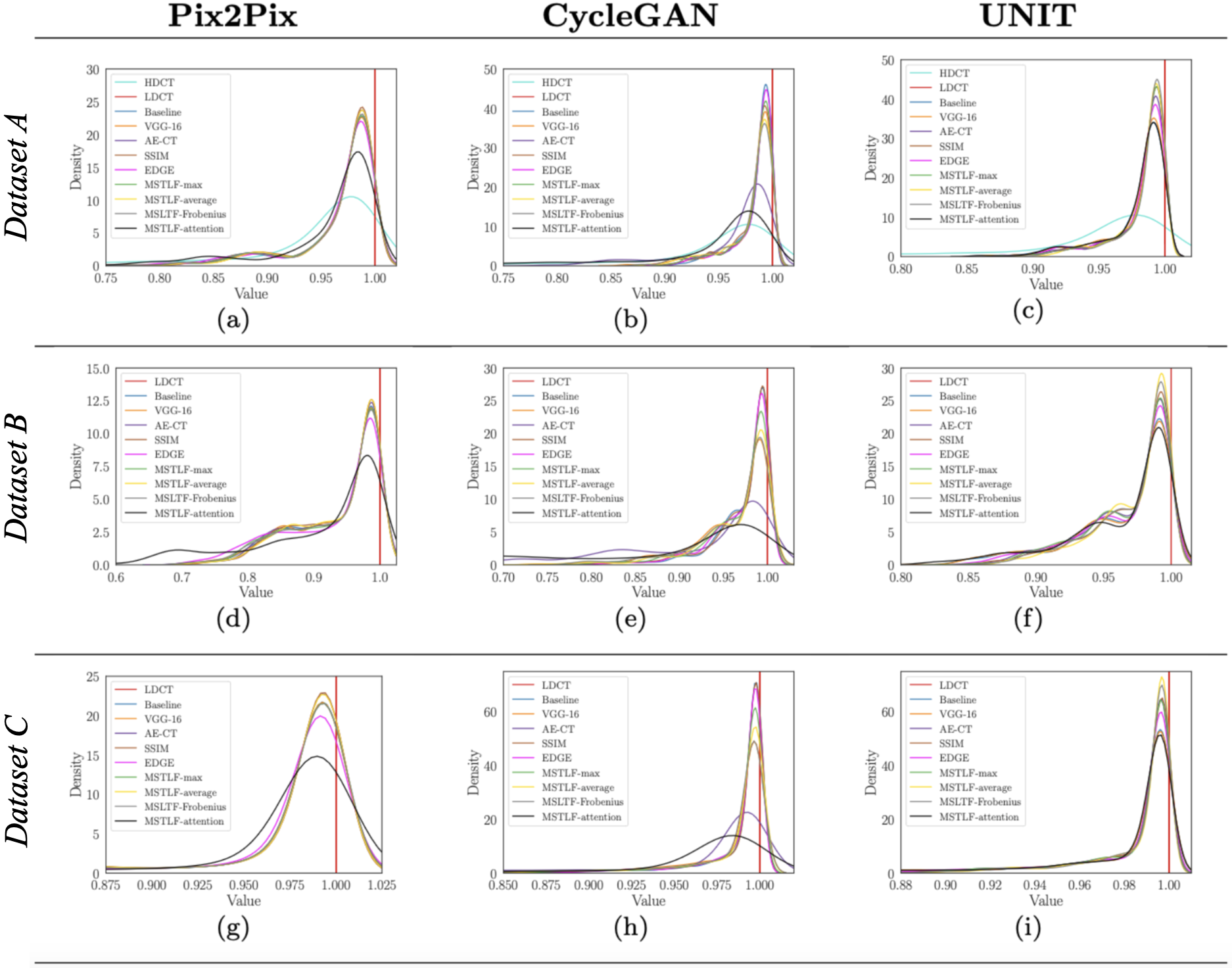
Figure 5: Template matching analysis. Each panel illustrates the matching distributions between the noisy templates extracted from the LDCT images and the denoised images.

4.3 Computational Analysis

Table 6 shows the computational analysis, where the computation time is given by the average time over one training epoch needed to compute the loss function and to back-propagate its gradient. In general, both CycleGAN and UNIT are more computationally demanding ($\sim 70\%$ more than Pix2Pix): this is expected since these two GANs have larger architectures than Pix2Pix, and also because they compute the loss term twice when performing the bidirectional translation between LD and HD domains. Both VGG-16 and AE-CT cause an increase in computational burden compared to the baseline (up to $+36\%$) since they use a VGG-16 network and an auto-encoder as feature extractors, respectively. Although these networks are frozen, the back-propagation is always computed, hence affecting the overall computation time. On the contrary, SSIM-L and EDGE have the same computation time as the baseline since they introduce two loss terms that rely on mathematical operations applied to the images without additional cost for back-propagating the gradient. Turning our attention to our MSTLFs, these cause a significant increase in computation time (up to $+65\%$ with respect to the baseline) due to the complexity of the operations that extract a multi-scale texture representation exploiting the soft GLCMs. Indeed, ensuring compatibility with the gradient-based optimization frameworks leads to an implementation that is more computationally onerous than the standard GLCM (section 2.3). Nonetheless, we notice that the type of aggregation used does not significantly affect the computational burden. In this regard, static aggregation, which is defined by mathematical operators, has the same impact as dynamic aggregation defined by self-attention. Such observation combined with the good performance reached by MSTLF-attention makes dynamic aggregation a promising approach.

Experiment	Pix2Pix	CycleGAN	UNIT
Baseline	0.09 s	0.42 s	0.28 s
VGG-16	0.13 s	0.49 s	0.44 s
AE-CT	0.11 s	0.47 s	0.41 s
SSIM	0.09 s	0.42 s	0.28 s
EDGE	0.09 s	0.42 s	0.28 s
MSTLF-max	0.26 s	0.89 s	0.81 s
MSTLF-average	0.26 s	0.94 s	0.82 s
MSTLF-Frobenius	0.26 s	0.95 s	0.82 s
MSTLF-attention	0.26 s	1.01 s	0.84 s

Table 6: Computational analysis. The computation time is expressed as the average time required to compute the loss function and to back-propagate its gradient for each batch.

5 Conclusions

In this paper, we present an approach, named MSTLF, for GAN-based denoising in CT imaging that embeds textural information, extracted at different spatial and angular scales. We also overcome the limitations posed by the non-differentiability of the GLCM proposing a novel implementation based on soft assignment that makes it compatible with gradient-based optimization frameworks. Our comprehensive analysis on three datasets and three GANs backbones brings out the effectiveness of MSTLF to enhance the quality of LDCT images. In particular, the configuration exploiting the attention layer to dynamically aggregate multi-scale texture data attains the best performance compared to other well-established loss functions. We also find two other interesting results. First, it also successfully tackles the challenging trade-off between distortion and perception. Second, just as it tailors the aggregation to the specific needs of the optimization process, it also succeeds in adapting the GAN architecture used. Future works are directed towards further investigation of the backbone-independent feature of the MSTLF, testing its application in other denoising frameworks in medical and non-medical applications.

References

- Aharon et al. [2006] Aharon, M., Elad, M., Bruckstein, A., 2006. K-SVD: An algorithm for designing overcomplete dictionaries for sparse representation. IEEE Transactions on signal processing 54, 4311–4322.
- Armato III [2011] Armato III, Samuel G, M., 2011. The lung image database consortium (LIDC) and image database resource initiative (IDRI): a completed reference database of lung nodules on CT scans. Medical physics 38, 915–931.
- Bera and Biswas [2023] Bera, S., Biswas, P.K., 2023. Self Supervised Low Dose Computed Tomography Image Denoising Using Invertible Network Exploiting Inter Slice Congruence, in: Proceedings of the IEEE/CVF Winter Conference on Applications of Computer Vision, pp. 5614–5623.
- Bevelacqua [2010] Bevelacqua, J.J., 2010. Practical and effective ALARA. Health physics 98, S39–S47.
- Blau and Michaeli [2018] Blau, Y., Michaeli, T., 2018. The perception-distortion tradeoff, in: Proceedings of the IEEE conference on computer vision and pattern recognition, pp. 6228–6237.
- Brenner and Hall [2007] Brenner, D.J., Hall, E.J., 2007. Computed tomography—an increasing source of radiation exposure. New England journal of medicine 357, 2277–2284.
- Burgos and Svoboda [2022] Burgos, N., Svoboda, D., 2022. Biomedical Image Synthesis and Simulation: Methods and Applications. Academic Press.
- Charbonnier et al. [1994] Charbonnier, P., Blanc-Feraud, L., Aubert, G., Barlaud, M., 1994. Two deterministic half-quadratic regularization algorithms for computed imaging, in: Proceedings of 1st international conference on image processing, IEEE. pp. 168–172.
- Dabov et al. [2007] Dabov, K., Foi, A., Katkovnik, V., Egiazarian, K., 2007. Image denoising by sparse 3-D transform-domain collaborative filtering. IEEE Transactions on image processing 16, 2080–2095.
- Depeursinge et al. [2017] Depeursinge, A., Omar, S., Al, K., Mitchell, J.R., 2017. Biomedical texture analysis: fundamentals, tools and challenges. Academic Press.
- Di Feola et al. [2023] Di Feola, F., Tronchin, L., Soda, P., 2023. A comparative study between paired and unpaired image quality assessment in low-dose ct denoising, in: 2023 IEEE 36th International Symposium on Computer-Based Medical Systems (CBMS), pp. 471–476. doi:10.1109/CBMS58004.2023.00264.
- Du et al. [2019] Du, W., Chen, H., Liao, P., Yang, H., Wang, G., Zhang, Y., 2019. Visual attention network for low-dose CT. IEEE Signal Processing Letters 26, 1152–1156.
- Elad et al. [2023] Elad, M., Kawar, B., Vaksman, G., 2023. Image denoising: The deep learning revolution and beyond—a survey paper. SIAM Journal on Imaging Sciences 16, 1594–1654.
- Gajera et al. [2021] Gajera, B., Kapil, S.R., Ziaei, D., Mangalagiri, J., Siegel, E., Chapman, D., 2021. CT-scan denoising using a charbonnier loss generative adversarial network. IEEE Access 9, 84093–84109.
- Gatys et al. [2015] Gatys, L., Ecker, A.S., Bethge, M., 2015. Texture synthesis using convolutional neural networks. Advances in neural information processing systems 28.
- Han et al. [2021] Han, M., Shim, H., Baek, J., 2021. Low-dose CT denoising via convolutional neural network with an observer loss function. Medical physics 48, 5727–5742.
- Han et al. [2022] Han, M., Shim, H., Baek, J., 2022. Perceptual CT loss: implementing CT image specific perceptual loss for CNN-based low-dose CT denoiser. IEEE Access 10, 62412–62422.
- Huang et al. [2021] Huang, Z., Zhang, J., Zhang, Y., Shan, H., 2021. DU-GAN: Generative adversarial networks with dual-domain U-Net-based discriminators for low-dose CT denoising. IEEE Transactions on Instrumentation and Measurement 71, 1–12.
- Isola et al. [2017] Isola, P., Zhu, J.Y., Zhou, T., Efros, A.A., 2017. Image-to-image translation with conditional adversarial networks, in: Proceedings of the IEEE conference on computer vision and pattern recognition, pp. 1125–1134.
- Izadi et al. [2023] Izadi, S., Sutton, D., Hamarneh, G., 2023. Image denoising in the deep learning era. Artificial Intelligence Review 56, 5929–5974.
- Johnson et al. [2016] Johnson, J., Alahi, A., Fei-Fei, L., 2016. Perceptual losses for real-time style transfer and super-resolution, in: Computer Vision–ECCV 2016: 14th European Conference, Amsterdam, The Netherlands, October 11-14, 2016, Proceedings, Part II 14, Springer. pp. 694–711.
- Kang et al. [2023] Kang, J., Liu, Y., Shu, H., Guo, N., Zhang, Q., Zhou, Y., Gui, Z., 2023. Gradient extraction based multiscale dense cross network for LDCT denoising. Nuclear Instruments and Methods in Physics Research Section A: Accelerators, Spectrometers, Detectors and Associated Equipment 1055, 168519.
- Kaur and Dong [2023] Kaur, A., Dong, G., 2023. A complete review on image denoising techniques for medical images. Neural Processing Letters 55, 7807–7850.
- Kingma and Ba [2014] Kingma, D.P., Ba, J., 2014. Adam: A method for stochastic optimization. arXiv preprint arXiv:1412.6980 .
- Kwon and Ye [2021] Kwon, T., Ye, J.C., 2021. Cycle-free cyclegan using invertible generator for unsupervised low-dose ct denoising. IEEE Transactions on Computational Imaging 7, 1354–1368.
- Kyung et al. [2022] Kyung, S., Won, J., Pak, S., Hong, G.s., Kim, N., 2022. MTD-GAN: Multi-task Discriminator Based Generative Adversarial Networks for Low-Dose CT Denoising, in: International Workshop on Machine Learning for Medical Image Reconstruction, Springer. pp. 133–144.
- Li et al. [2020a] Li, M., Hsu, W., Xie, X., Cong, J., Gao, W., 2020a. SACNN: Self-attention convolutional neural network for low-dose CT denoising with self-supervised perceptual loss network. IEEE transactions on medical imaging 39, 2289–2301.
- Li et al. [2022] Li, S., Li, Q., Li, R., Wu, W., Zhao, J., Qiang, Y., Tian, Y., 2022. An adaptive self-guided wavelet convolutional neural network with compound loss for low-dose CT denoising. Biomedical Signal Processing and Control 75, 103543.
- Li et al. [2023] Li, Z., Liu, Y., Shu, H., Lu, J., Kang, J., Chen, Y., Gui, Z., 2023. Multi-Scale Feature Fusion Network for Low-Dose CT Denoising. Journal of Digital Imaging , 1–18.
- Li et al. [2021] Li, Z., Shi, W., Xing, Q., Miao, Y., He, W., Yang, H., Jiang, Z., 2021. Low-dose CT image denoising with improving WGAN and hybrid loss function. Computational and Mathematical Methods in Medicine 2021.
- Li et al. [2020b] Li, Z., Zhou, S., Huang, J., Yu, L., Jin, M., 2020b. Investigation of low-dose CT image denoising using unpaired deep learning methods. IEEE transactions on radiation and plasma medical sciences 5, 224–234.
- Liu et al. [2017] Liu, M.Y., Breuel, T., Kautz, J., 2017. Unsupervised image-to-image translation networks. Advances in neural information processing systems 30.
- Ma et al. [2020] Ma, Y., Wei, B., Feng, P., He, P., Guo, X., Wang, G., 2020. Low-dose CT image denoising using a generative adversarial network with a hybrid loss function for noise learning. IEEE Access 8, 67519–67529.
- Marcos et al. [2021] Marcos, L., Alirezaie, J., Babyn, P., 2021. Low dose CT image denoising using boosting attention fusion gan with perceptual loss, in: 2021 43rd Annual International Conference of the IEEE Engineering in Medicine & Biology Society (EMBC), IEEE. pp. 3407–3410.
- Matsoukas et al. [2022] Matsoukas, C., Haslum, J.F., Sorkhei, M., Söderberg, M., Smith, K., 2022. What makes transfer learning work for medical images: Feature reuse & other factors, in: Proceedings of the IEEE/CVF Conference on Computer Vision and Pattern Recognition, pp. 9225–9234.
- Mittal Anish [2012] Mittal Anish, Rajiv Soundararajan, A.C.B., 2012. Making a “completely blind” image quality analyzer. IEEE Signal processing letters 20, 209–212.
- Moen et al. [2021] Moen, T.R., Chen, B., Holmes III, D.R., Duan, X., Yu, Z., Yu, L., Leng, S., Fletcher, J.G., McCollough, C.H., 2021. Low-dose CT image and projection dataset. Medical physics 48, 902–911.
- Ohno et al. [2019] Ohno, Y., Koyama, H., Seki, S., Kishida, Y., Yoshikawa, T., 2019. Radiation dose reduction techniques for chest CT: principles and clinical results. European journal of radiology 111, 93–103.
- Pan et al. [2020] Pan, Z., Yu, W., Wang, B., Xie, H., Sheng, V.S., Lei, J., Kwong, S., 2020. Loss functions of generative adversarial networks (GANs): Opportunities and challenges. IEEE Transactions on Emerging Topics in Computational Intelligence 4, 500–522.
- Pang et al. [2021] Pang, Y., Lin, J., Qin, T., Chen, Z., 2021. Image-to-image translation: Methods and applications. IEEE Transactions on Multimedia 24, 3859–3881.
- Park et al. [2019] Park, H.S., Baek, J., You, S.K., Choi, J.K., Seo, J.K., 2019. Unpaired image denoising using a generative adversarial network in X-ray CT. IEEE Access 7, 110414–110425.
- Park et al. [2022] Park, H.S., Jeon, K., Lee, J., You, S.K., 2022. Denoising of pediatric low dose abdominal CT using deep learning based algorithm. Plos one 17, e0260369.
- Russakovsky et al. [2015] Russakovsky, O., Deng, J., Su, H., Krause, J., Satheesh, S., Ma, S., Huang, Z., Karpathy, A., Khosla, A., Bernstein, M., Berg, F.F., 2015. Imagenet large scale visual recognition challenge. International journal of computer vision 115, 211–252.
- Santucci et al. [2021] Santucci, D., Faiella, E., Cordelli, E., Sicilia, R., de Felice, C., Zobel, B.B., Iannello, G., Soda, P., 2021. 3T MRI-radiomic approach to predict for lymph node status in breast cancer patients. Cancers 13, 2228.
- Scott [2015] Scott, D.W., 2015. Multivariate density estimation: theory, practice, and visualization. John Wiley & Sons.
- Simonyan and Zisserman [2014] Simonyan, K., Zisserman, A., 2014. Very deep convolutional networks for large-scale image recognition. arXiv preprint arXiv:1409.1556 .
- Tan et al. [2022] Tan, C., Yang, M., You, Z., Chen, H., Zhang, Y., 2022. A selective kernel-based cycle-consistent generative adversarial network for unpaired low-dose CT denoising. Precision Clinical Medicine 5, pbac011.
- Tronchin et al. [2021] Tronchin, L., Sicilia, R., Cordelli, E., Ramella, S., Soda, P., 2021. Evaluating GANs in medical imaging, in: Deep Generative Models, and Data Augmentation, Labelling, and Imperfections: First Workshop, MICCAI 2021, Proceedings, Springer. pp. 112–121.
- Venkatanath et al. [2015] Venkatanath, N., Praneeth, D., Bh, M.C., Channappayya, S.S., Medasani, S.S., 2015. Blind image quality evaluation using perception based features, in: 2015 twenty first national conference on communications (NCC), IEEE. pp. 1–6.
- Vision and I. A. Group [2009] Vision and I. A. Group, 2009. VIA/I-ELCAP public access research database. http://www.via.cornell.edu/databases/lungdb.html. Accessed April 7, 2009.
- Wang et al. [2004] Wang, Z., Bovik, A.C., Sheikh, H.R., Simoncelli, E.P., 2004. Image quality assessment: from error visibility to structural similarity. IEEE transactions on image processing 13, 600–612.
- Wolterink et al. [2017] Wolterink, J.M., Leiner, T., Viergever, M.A., Išgum, I., 2017. Generative adversarial networks for noise reduction in low-dose CT. IEEE transactions on medical imaging 36, 2536–2545.
- Yang et al. [2023] Yang, L., Liu, H., Shang, F., Liu, Y., 2023. Adaptive Non-Local Generative Adversarial Networks for Low-Dose CT Image Denoising, in: ICASSP 2023-2023 IEEE International Conference on Acoustics, Speech and Signal Processing (ICASSP), IEEE. pp. 1–5.
- Yang et al. [2018] Yang, Q., Yan, P., Zhang, Y., Yu, H., Shi, Y., Mou, X., Kalra, M.K., Zhang, Y., Sun, L., Wang, G., 2018. Low-dose CT image denoising using a generative adversarial network with Wasserstein distance and perceptual loss. IEEE transactions on medical imaging 37, 1348–1357.
- Yin et al. [2021] Yin, Z., Xia, K., He, Z., Zhang, J., Wang, S., Zu, B., 2021. Unpaired image denoising via Wasserstein GAN in low-dose CT image with multi-perceptual loss and fidelity loss. Symmetry 13, 126.
- Yin et al. [2023] Yin, Z., Xia, K., Wang, S., He, Z., Zhang, J., Zu, B., 2023. Unpaired low-dose CT denoising via an improved cycle-consistent adversarial network with attention ensemble. The Visual Computer 39, 4423–4444.
- You et al. [2018] You, C., Yang, Q., Shan, H., Gjesteby, L., Li, G., Ju, S., Zhang, Z., Zhao, Z., Zhang, Y., Cong, W., Weng, 2018. Structurally-sensitive multi-scale deep neural network for low-dose CT denoising. IEEE access 6, 41839–41855.
- Zamir et al. [2021] Zamir, S.W., Arora, A., Khan, S., Hayat, M., Khan, F.S., Yang, M.H., Shao, L., 2021. Multi-stage progressive image restoration, in: Proceedings of the IEEE/CVF conference on computer vision and pattern recognition, pp. 14821–14831.
- Zhang et al. [2019] Zhang, H., Goodfellow, I., Metaxas, D., Odena, A., 2019. Self-attention generative adversarial networks, in: International conference on machine learning, PMLR. pp. 7354–7363.
- Zhao et al. [2016] Zhao, H., Gallo, O., Frosio, I., Kautz, J., 2016. Loss functions for image restoration with neural networks. IEEE Transactions on computational imaging 3, 47–57.
- Zhu et al. [2017] Zhu, J.Y., Park, T., Isola, P., Efros, A.A., 2017. Unpaired image-to-image translation using cycle-consistent adversarial networks, in: Proceedings of the IEEE international conference on computer vision, pp. 2223–2232.