Symbolic and User-friendly Geometric Algebra Routines ($\mathtt{SUGAR}$) for Computations in Matlab

Abstract.

Geometric algebra (GA) is a mathematical tool for geometric computing, providing a framework that allows a unified and compact approach to geometric relations which in other mathematical systems are typically described using different more complicated elements. For instance, in robotics, where conventional formulations rely on coordinate-based approaches involving matrix multiplication, GA simplifies the process to the multiplication of special elements, called rotors. This efficiency has led to an increasing adoption of GA in applied mathematics and engineering problems. However, the scarcity of symbolic implementations of GA and its inherent complexity, requiring a specific mathematical background, make it challenging and less intuitive for engineers to work with. This prevents wider adoption among more applied professionals. To address this challenge, this paper introduces $\mathtt{SUGAR}$ (Symbolic and User-friendly Geometric Algebra Routines), an open-source toolbox designed for Matlab and licensed under the MIT License. $\mathtt{SUGAR}$ facilitates the translation of GA concepts into Matlab and provides a collection of user-friendly functions tailored for GA computations, including support for symbolic operations. It supports both numeric and symbolic computations in high-dimensional GAs. Specifically tailored for applied mathematics and engineering applications, $\mathtt{SUGAR}$ has been meticulously engineered to represent geometric elements and transformations within two and three-dimensional projective and conformal geometric algebras, aligning with established computational methodologies in the literature. Furthermore, $\mathtt{SUGAR}$ efficiently handles functions of multivectors, such as exponential, logarithmic, sinusoidal, and cosine functions, enhancing its applicability across various engineering domains, including robotics, control systems, and power electronics. Finally, this work includes four distinct validation examples, demonstrating SUGAR’s capabilities across the above-mentioned fields and its practical utility in addressing real-world applied mathematics and engineering problems.

1. Introduction

From an applied mathematics and engineering perspective, geometric algebra (GA) (Hestenes and Sobczyk, 1984) can be described as a mathematical tool for geometric computing, as it provides a framework that allows a unified and compact approach to geometric relations which in other mathematical systems are typically described using different elements. An illustration of this occurs in the field of robotics (Bayro-Corrochano, 2020), where the end-effector’s position is a Euclidean point, while its orientation is represented by a quaternion. In GA, however, both can be represented as a single element, referred to as a multivector. Projective or Plane-based Geometric Algebra (PGA) and Conformal Geometric Algebra (CGA) (Hestenes, 2001) introduce an even more elegant and intuitive approach to geometry by encoding both the geometric entities (such as points, lines, planes and spheres) and geometric transformations (such as rotations and translations) as elements of the algebra, which in turn allows to operate with them as one does with real numbers. Beyond applied mathematics and engineering, GA also leads to the simplification of many otherwise complex equations, making them more intuitive and easy to handle. An example of this is seen in the well-known Maxwell equations, which can be reduced to a single equation using GA (Chappell et al., 2014).

The inherent geometric intuition and the potential for simplifying complex equations make GA relevant in various engineering fields. Disciplines with a predominant geometric interpretation like robotics already apply GA, PGA and CGA either in kinematics, dynamics, or tracking and control of robotic systems (Bayro-Corrochano, 2020; Lavor et al., 2018; Bayro-Corrochano et al., 2022; Löw and Calinon, 2023). In addition, since applied mathematicians and engineers are always interested in keeping equations as simple and compact as possible, the above-mentioned inherent simplifying feature of GA has attracted attention from other disciplines as well. This attraction has been reported in several surveys/tutorials. A survey of GA applications in fields such as signal and image processing, computer vision, and artificial intelligence can be found in (Hitzer et al., 2013). An updated survey targeting GA applications in computer science and engineering from 1995 to 2020 can be found in (Bayro-Corrochano, 2021), while a more specific introduction of GA to electrical en electronic engineers can be found in (Chappell et al., 2014).

This interest on GA, PGA and CGA triggers the need for software implementations where mathematicians and engineers may feel more comfortable. Motivated by this need, this paper presents an implementation of GA, PGA and CGA for Matlab^®. Matlab is a proprietary software system developed and sold by The MathWorks. It has been commercially available since 1984 and it is now considered as a standard tool at most universities and industries worldwide. Matlab is an interactive system whose basic data element is an array that does not require dimensioning, easing the calculus with matrices of real and complex numbers. Specific application domains are collected in packages referred to as toolboxes, covering symbolic computation, control theory, simulation, optimization, and several other fields of applied science and engineering.

The GA, PGA, and CGA implementation presented in this paper is given under the $\mathtt{SUGAR}$ toolbox (Velasco, 2023), that stands for Symbolic and User-friendly Geometric Algebra Routines. The name aims to stress two of SUGAR’s key features. The first one is its capability to allow symbolic computations (which makes it unique), scaling to any (high) dimension (where the limitation is the CPU power, but not the underlying algorithmics). The second one refers to the fact that it has been developed to offer a more natural language that can be directly applied to complex problems in both applied mathematics and engineering, thus easing its usage and speeding-up its learning curve, that is, being user-friendly.

It is interesting to note that $\mathtt{SUGAR}$ was born for covering the specific research needs faced in the modeling, analysis and control of (unbalanced) three-phase electrical systems (Velasco et al., 2023). However, the rapid interest on the few original routines that was shown by GA-research colleagues triggered a new coding effort that lead to the current version of $\mathtt{SUGAR}$, serving different fields, as illustrated in the application examples presented at the end of the present article.

The rest of this manuscript is organized as follows. First, Section 2 provides a brief introduction to geometric algebra, as well as projective and conformal geometric algebras, to establish the foundation for understanding the rest of the manuscript. Section 3 presents a non-exhaustive state-of-the-art analysis of available geometric algebra-related software implementations. Then, Section 4 describes the main features of $\mathtt{SUGAR}$, as well as the initial steps to utilize these features. Finally, Section 5 presents application examples, and Section 6 concludes the paper.

2. A primer on GA

In this section, a brief introduction to GA, PGA and CGA is provided. Readers interested in a more detailed treatment of the subject are referred to the classical texts (Hestenes and Sobczyk, 1984; Hestenes, 2001; Doran and Lasenby, 2003; Dorst and Keninck, 2022).

2.1. Geometric algebra

Let $\mathbb{R}^{p,q,r}$ be a the pseudo-Euclidean space with orthonormal basis $\{e_{1},\dots,e_{p},e_{p+1},\dots,e_{p+q},e_{p+q+1},\dots,e_{p+q+r}\}$, where the basis elements $\{e_{1},\dots,e_{p}\}$ square to $1$, the basis elements $\{e_{p+1},\dots,e_{p+q}\}$ square to $-1$, and the basis elements $\{e_{p+q+1},\dots,e_{p+q+r}\}$ square to $0$. The geometric algebra of $\mathbb{R}^{p,q,r}$, denoted by $\mathcal{G}_{p,q,r}$, is a vector space where the operations defined in $\mathbb{R}^{p,q,r}$, i.e., the addition and multiplication by scalars, are extended naturally. An additional operation, the geometric product, is defined, and acts on vectors of the algebra as follows:

(1) $$v_{1}v_{2}=v_{1}\cdot v_{2}+v_{1}\wedge v_{2},\,\text{ for }v_{1},v_{2}\in\mathbb{R}^{p,q,r},$$

where $\cdot$ denotes the inner or dot product and $\wedge$ denotes the outer product.

The outer product of two vectors $v_{1},v_{2}$ is a new element of $\mathcal{G}_{p,q,r}$, which is termed a bivector, is said to have grade two and is denoted by $v_{1}\wedge v_{2}$. By extension, the outer product of a bivector with a vector is known as a trivector and is denoted by $(v_{1}\wedge v_{2})\wedge v_{3}$. Clearly, trivectors have grade three. This can be generalized to an arbitrary dimension. Thus,

(2) $$(v_{1}\wedge v_{2}\wedge\dots\wedge v_{k-1})\wedge v_{k}$$

denotes an $k$-blade, an element of $\mathcal{G}_{p,q,r}$ with grade $k$.

A bivector $v_{1}\wedge v_{2}$ can be interpreted as the oriented area defined by the vectors $v_{1}$ and $v_{2}$. Thus, $v_{2}\wedge v_{1}$ has opposite orientation and, from that, the anticommutativity of the outer product can be deduced. Analogously, a trivector is interpreted as the oriented volume defined by its three composing vectors. Since the volume generated by $(v_{1}\wedge v_{2})\wedge v_{3}$ is the same as the volume generated by $v_{1}\wedge(v_{2}\wedge v_{3})$, it is also deduced that the outer product is associative. Therefore, $k$-blades can be denoted simply as:

(3) $$v_{1}\wedge v_{2}\wedge\dots\wedge v_{k}.$$

Linear combinations of $k$-blades are known as $k$-vectors, while linear combinations of $k$-vectors, for $0\leq k\leq p+q+r$, are called multivectors. Multivectors are the most important elements of geometric algebra.

Applied to the basis elements $\{e_{i}\}$, the geometric product acts as follows:

(4) $$e_{i}e_{j}=\left\{\begin{array}[]{lcl}1&\text{for}&i=j\text{ and }i\leq p\\ -1&\text{for}&i=j\text{ and }p<i\leq p+q\\ 0&\text{for}&i=j\text{ and }p+q<i\leq p+q+r\\ e_{i}\wedge e_{j}&\text{for}&i\neq j\end{array}\right.$$

Then, $\{e_{1},\dots,e_{p},e_{p+1},\dots,e_{p+q},e_{p+q+1},\dots,e_{p+q+r}\}$ can be expanded to a basis of $\mathcal{G}_{p,q,r}$ that contains, for each $0\leq k\leq p+q+r$, $C(p+q+r,k)$ grade $k$ elements:

(5) $$\begin{split}&\text{Scalar: }1\\ &\text{Vectors: }e_{1},\dots,e_{p+q+r}\\ &\text{Bivectors: }\{e_{i}\wedge e_{j}\}_{1\leq i<j\leq p+q+r}\\ &\text{Trivectors: }\{e_{i}\wedge e_{j}\wedge e_{k}\}_{1\leq i<j<k\leq p+q+r}\\ &\vdots\\ &k-\text{vectores: }\{e_{i_{1}}\wedge\dots\wedge e_{i_{k}}\}_{1\leq i_{1}<\dots<i_{k}\leq n}\\ &\vdots\\ &\text{$p+q+r$-blade: }e_{1}\wedge\dots\wedge e_{p+q+r}\end{split}$$

which sums up to total of $2^{p+q+r}$ elements. Understanding how the geometric product acts on the basis elements of $\mathcal{G}_{p,q,r}$ allows for its extension to arbitrary multivectors. The grade $p+q+r$ element $e_{1}\wedge\dots\wedge e_{p+q+r}$ is known as the pseudoscalar and is usually denoted by $I$. If $r=0$, pseudoscalars allow for the definition of one of the main operators of geometric algebra, the dual operator. Its action over an $k$-vector $A_{k}$ is:

(6) $$A_{k}^{\ast}=A_{k}I,$$

where $A_{k}^{\ast}$ is an $(p+q-k)$-vector. In particular, for two multivectors $A$ and $B$, the following identity holds:

(7) $$(A\wedge B)^{\ast}=A\cdot B^{\ast}.$$

Among all geometric algebras, the most interesting ones are those with $p=n$ and $q=r=0$, i.e., geometric algebras over an $n$-dimensional Euclidean space $\mathbb{R}^{n}$. These are denoted $\mathcal{G}_{n}$ for $n\in\mathbb{N}$. The bivectors of $\mathcal{G}_{n}$ play an important role since they can be used to describe $n$-dimensional rotations. Indeed, in geometric algebra, rotations are described using rotors. If a point $x\in\mathbb{R}^{n}$ is rotated by an angle $\theta$ around an axis $\ell$, the rotor $R$ defining such a rotation in $\mathcal{G}_{n}$ is:

(8) $$R=e^{-\frac{\theta}{2}B}=\cos\biggl{(}\dfrac{\theta}{2}\biggr{)}-\sin\biggl{(}\dfrac{\theta}{2}\biggr{)}B,$$

where $B$ is the unit bivector, i.e., $B^{2}=-1$, representing the hyperplane normal to $\ell$. The second identity is obtained by expanding the Taylor series of the exponential $e^{-\frac{\theta}{2}B}$ and regrouping terms (more details can be found in (Doran and Lasenby, 2003)). The rotated point $x^{\prime}$ is calculated by sandwiching $x$ between $R$ and its reverse $\widetilde{R}$:

(9) $$x^{\prime}=Rx\widetilde{R}$$

where

(10) $$\widetilde{R}=\cos\biggl{(}\dfrac{\theta}{2}\biggr{)}+\sin\biggl{(}\dfrac{\theta}{2}\biggr{)}B$$

and $R\widetilde{R}=1$. Furthermore, equation (9) can be extended to arbitrary multivectors. In addition, to specify what unit multivectors are, a norm is defined in $\mathcal{G}_{n}$. For an arbitrary multivector $A$, it is:

(11) $$\|A\|=\sqrt{\left<A\widetilde{A}\right>_{0}},$$

where $\left<\cdot\right>_{0}$ is the grade-0 projection operator, i.e., it extracts the scalar elements of the argument multivector. In fact, grade-$k$ projection operators constitute an important family of linear operators in $\mathcal{G}_{n}$. They are denoted by $\left<\cdot\right>_{k}$ for $0\leq k\leq n$. When applied to an arbitrary multivector $A$, $\left<A\right>_{k}$ projects onto the grade-$k$ components in $A$, i.e., it returns the components of $A$ that can be expressed as a linear combination of $\{e_{i_{1}}\wedge\dots\wedge e_{i_{k}}\}_{1\leq i_{1}<\dots<i_{k}\leq n}$. Obviously, if $A_{k}$ denotes a $k$-vector, then $\left<A_{k}\right>_{k}=A_{k}$.

Using these operators, general multivectors $A\in\mathcal{G}_{n}$ can be expressed as:

(12) $$A=\left<A\right>_{0}+\left<A\right>_{1}+\dots+\left<A\right>_{n}.$$

Hence, the set of all $k$-vectors for a given $1\leq k\leq n$ is a vector subspace of $\mathcal{G}_{n}$ denoted by $\left<\mathcal{G}_{n}\right>_{k}$ and spanned by $B_{k}=\{e_{i_{1}}\wedge\dots\wedge e_{i_{k}}\}_{1\leq i_{1}<\dots<i_{k}\leq n}$.

The multivector representation (12) is very useful in defining another important operator in $\mathcal{G}_{n}$. This linear operator is known as the reversion operator and is denoted by the superscript $\sim$. The reversion is defined over the geometric product of $m$ vectors as:

(13) $$(a_{1}\cdots a_{m})^{\sim}=a_{m}\cdots a_{1}.$$

Applied to $k$-vectors:

(14) $$\widetilde{A}_{k}=(-1)^{\frac{k(k-1)}{2}}A_{k}$$

due to the anticommutativity of the outer product. Finally, since reversion is a linear operator, the reverse of an arbitrary multivector is:

(15) $$\widetilde{A}=\left<\widetilde{A}\right>_{0}+\dots+\left<\widetilde{A}\right>_{n}=\left<A\right>_{0}+\left<A\right>_{1}-\left<A\right>_{2}+\dots+(-1)^{\frac{n(n-1)}{2}}\left<A\right>_{n}.$$

2.2. Projective geometric algebra

The projective or plane-based model extends the $n$-dimensional Euclidean space $\mathbb{R}^{n}$ by adding an extra basis vector $e$ with the property $e^{2}=0$, i.e., vector $e$ is a null vector. This null vector is associated with the point at infinity (and this is why this geometric algebra is known as the projective geometric algebra).

The projective or plane-based geometric algebra (PGA) of $\mathbb{R}^{n}$, denoted $\mathcal{G}_{n,0,1}$, can be seen as the geometric algebra of $\mathbb{R}^{n,0,1}$. One of the key features of PGA is that it allows the encoding of translations as rotors. Thus, all proper rigid body transformations are represented by the same structure within the algebra. This property enables the use of PGA in kinematic-related problems, such as in robotics. In particular, the addition of the null basis vector $e$ allows for the definition of null bivectors of the form $B=b\wedge e$, where $b$ is a non-null vector of $\mathbb{R}^{n}$. These bivectors simplify the Taylor expansion of $e^{-\frac{\theta}{2}B}$ to a single linear term of the form:

(16) $$e^{-\frac{\theta}{2}B}=1-\dfrac{b\wedge e}{2}$$

which encodes a rotation around a line with one point at infinity, i.e., a translation along the direction vector $b\in\mathbb{R}^{n}$. These rotors are denoted as $T_{b}$, and they are applied to other vectors using the sandwich product, similar to any other rotor. In other words, to translate vector $x$ along the direction $b$:

(17) $$x^{\prime}=T_{b}x\widetilde{T}_{b},$$

where $x^{\prime}$ is the translated vector and $\widetilde{T}=1+\frac{b\wedge e}{2}$.

Finally, the pseudoscalar for this algebra is $I=e_{1}e_{2}\dots e_{n}e$, which, due to the null vector $e$, satisfies $I^{2}=0$. Therefore, it is not suitable to compute the dual using that pseudoscalar. Instead, the pseudoscalar used in PGA is $\mathcal{I}=\widetilde{I_{n}}\wedge e^{r}$, where $\widetilde{I_{n}}$ is the reverse of the pseudoscalar of $\mathcal{G}_{n}$ and $e^{r}$ is the reciprocal of the basis element $e$, i.e., $e^{r}$ is such that $e\cdot e^{r}=1$ (a more detailed explanation can be found in (Dorst and Keninck, 2022)).

2.3. Conformal geometric algebra

The conformal model extends the $n$-dimensional Euclidean space $\mathbb{R}^{n}$ by adding two extra basis vectors, $e$ and $\overline{e}$, with the property:

(18) $$e^{2}=1,\quad\overline{e}^{2}=-1.$$

These two extra vectors allow the definition of two null vectors:

(19) $$n_{0}=\dfrac{1}{2}\left(\overline{e}+e\right),\quad n_{\infty}=\overline{e}-e,$$

where $n_{\infty}$ is associated with the point at infinity and $n_{0}$ with the origin.

Thus, the conformal geometric algebra (CGA) of $\mathbb{R}^{n}$ is denoted by $\mathcal{G}_{n+1,1}$ and can be seen as the geometric algebra of $\mathbb{R}^{n+1,1}$. Now, the two null vectors $n_{\infty}$ and $n_{0}$ allow an intuitive description of translations, that are formulated as rotors in the same way as in PGA:

(20) $$T_{v}=1-\dfrac{v\wedge n_{\infty}}{2},$$

where the translation is performed in the direction of $v\in\mathbb{R}^{n}$.

One of the most important advantages of conformal geometric algebra is that it provides a homogeneous model for the $n$-dimensional Euclidean space. In particular, every point $x\in\mathbb{R}^{n}$ is associated with a null vector of $\mathcal{G}_{n+1,1}$ (including the origin and the point at the infinity). This is done via the Hestenes’ embedding:

(21) $$\bm{x}=H(x)=\dfrac{1}{2}x^{2}n_{\infty}+n_{0}+x,$$

where $\bm{x}$ is said to be the null vector representation of $x$. The inverse of the Hestenes’ embedding is just the projection operator onto $\mathbb{R}^{n}$.

Another key feature of CGA is that it encodes geometric entities as elements of the algebra. In particular, the geometric entities of the conformal model of $\mathbb{R}^{3}$, $\mathcal{G}_{4,1}$, are considered, including points, lines, planes, circles and spheres. If $O$ denotes a geometric entity, then $\bm{o}$ is said to be the outer representation of $O$ if for every point $x\in O$, $\bm{x}\wedge\bm{o}=0$. Taking the dual of the outer representation $\bm{o}$ of a geometric entity $O$, the inner representation $\bm{o}^{\ast}$ is obtained. The inner representation satisfies $\bm{x}\cdot\bm{o}^{\ast}=0$ for a null vector representation of $x\in O$.

Now, for two different geometric objects $O_{1}$ and $O_{2}$ with outer (inner) representations $\bm{o}_{1}$ and $\bm{o}_{2}$ ($\bm{o}_{1}^{\ast}$ and $\bm{o}_{2}^{\ast}$), their intersection, denoted by $\bm{o}_{1}\vee\bm{o}_{2}$, is the multivector:

(22) $$\bm{o}_{1}\vee\bm{o}_{2}=(\bm{o}_{1}^{\ast}\wedge\bm{o}_{2}^{\ast})^{\ast}.$$

Analogously, if the outer representations of $O_{1}$ and $O_{2}$ have the same grade, the angle defined by them is computed as follows:

(23) $$\angle(O_{1},O_{2})=\cos^{-1}\left(\dfrac{\bm{o}_{1}\cdot\bm{o}_{2}}{\sqrt{\bm{o}_{1}\widetilde{\bm{o}_{1}}}\sqrt{\bm{o}_{2}\widetilde{\bm{o}_{2}}}}\right).$$

To describe the different geometric entities, let $p_{1},p_{2},p_{3},p_{4}\in\mathbb{R}^{3}$ be four different points with null vector representation $\bm{p}_{1},\bm{p}_{2},\bm{p}_{3},\bm{p}_{4}\in\mathcal{G}_{4,1}$. Then:

• $\bm{b}=\bm{p}_{1}\wedge\bm{p}_{2}$ is a bivector and the outer representation of the pair of points $p_{1}$ and $p_{2}$.

• $\bm{\ell}=\bm{p}_{1}\wedge\bm{p}_{2}\wedge e_{\infty}$ is a trivector and the outer representation of the line passing through the points $p_{1}$ and $p_{2}$. Its inner representation is the bivector $\bm{\ell}^{\ast}=ve_{123}-(p_{1}\wedge v)e_{123}e_{\infty}$, where $v=p_{1}-p_{2}$ is its direction vector.

• $\bm{c}=\bm{p}_{1}\wedge\bm{p}_{2}\wedge\bm{p}_{3}$ is a trivector and the outer representation of a circle passing through the points $p_{1},p_{2}$ and $p_{3}$. Its inner representation is the bivector $\bm{c}^{\ast}=\bm{\pi}^{\ast}\wedge\bm{s}^{\ast}$, where $\bm{\pi}^{\ast}$ and $\bm{s}^{\ast}$ are the inner representations of the plane and sphere whose intersection defines the circle.

• $\bm{\pi}=\bm{p}_{1}\wedge\bm{p}_{2}\wedge\bm{p}_{3}\wedge e_{\infty}$ is a 4-vector and the outer representation of a plane passing through the points $p_{1},p_{2}$ and $p_{3}$. Its inner representation is the vector $\bm{\pi}^{\ast}=n+\delta e_{\infty}$, where $n$ denotes the vector normal to the plane and $\delta$, its orthogonal distance to the origin.

• $\bm{s}=\bm{p}_{1}\wedge\bm{p}_{2}\wedge\bm{p}_{3}\wedge\bm{p}_{4}$ is a 4-vector and the outer representation of a sphere passing through the points $p_{1},p_{2},p_{3}$ and $p_{4}$. Its inner representation is the vector $\bm{s}^{\ast}=\bm{z}-\frac{1}{2}r^{2}e_{\infty}$, where $\bm{z}$ is the null vector representation of the center of the sphere and $r$, its radius.

3. State of the art

There is a wider offer of computational libraries and tools for computing with GA. Probably the first documented library is CLICAL, a stand-alone calculator-like program running under MS-DOS (Lounesto et al., 1987). From this pioneer approach, many complementary implementations have appeared. In the following, some of them are reviewed with the objective of positioning $\mathtt{SUGAR}$ in the map, which can be almost completely drawn using the geometric algebra explorer website that shares a long list of GA-inspired software.

Looking at GA implementations for programming languages, different options exist, such as $\mathtt{Versor}$ (Colapinto, 2011), a C++ library for geometric algebra, or $\mathtt{Ganja.js}$(De Keninck, 2017), a geometric algebra code generator for javascript capable of generating geometric algebras and subalgebras of any signature. $\mathtt{Ganja.js}$ also implements operator overloading and algebraic constraints. $\mathtt{GAlgebra}$ (Bromborsky and team, 2014) is an implementation of a geometric algebra module in python that utilizes the sympy symbolic algebra library. However, it does not handle projective or conformal geometric algebras and is not maintained since 2019. Additionally, $\mathtt{GMac}$ (Awad Eid, 2016), short form for ”Geometric Macro”, is a sophisticated .NET based code generation software system that allows implementing geometric models and algorithms based on GA in arbitrary target programming languages. These implementations, in general, target programming languages that are not very popular among engineers or mathematicians, that prefer for example VBA/VBS (scripting languages that stem from the Visual Basic programming) like MS Excel , Labview , or the already mentioned Matlab.

In other cases, GA is implemented using a specialized package, either symbolic or numeric, within a larger mathematical software system. For instance, $\mathtt{Clifford}$ (Prodanov and Toth, 2017) is a lightweight package for performing geometric algebra calculations in Maxima – a computer algebra system for the manipulation of symbolic and numerical expressions. $\mathtt{CLIFFORD}$ (Ablamowicz and Fauser, 2005) is a package for Clifford and Grassmann algebras computations within Maple – a symbolic and numeric computing environment, and $\mathtt{CGAlgebra}$ (Ortiz-Duran and Aragon, 2017) is a package for 5D conformal geometric algebra in Mathematica – a platform for technical computing that has been the basis for the development of the WolframAlpha answer engine.

Regarding Matlab, GABLE, which stands for Geometric Algebra Learning Environment, is the first geometric algebra package mentioned in the literature (Mann et al., 1999). However, its main limitation is that it only handles geometric algebras up to $p+q=3$. Additionally, it can only process single multivectors, i.e., it cannot handle arrays or matrices of multivectors. An additional implementation of a geometric algebra package is presented in (Antanovskii, 2014). This implementation covers basic algebraic operations, allowing symbolic manipulations, but it supports only up $p+q=4$. The limitation rises from the implementation of the algebraic operations, which are explicitly coded for each dimension. A qualitative progress is found in the Clifford Multivector Toolbox (Sangwine and Hitzer, 2016) (from the same authors of the Quaternion Toolbox for Matlab, QTM (Sangwine and Le Bihan, 2005)), which has been designed to extend Matlab in a natural Matlab-like manner to handle arrays (including, but not limited to, vectors and matrices) with elements which are Clifford o geometric multivectors in an arbitrarily chosen geometric algebra. The main limitation relies in the lack of support for symbolic computations. In addition, its treatment of PGA and CGA does not allow a full geometric interpretation of the manipulations of the special elements from those algebras, which may discourage mathematicians and engineers from using it. To fill this gap, $\mathtt{SUGAR}$ offers symbolic and numerical computations, permits operating with arrays or matrices of multivectors, and many of the functions that implements are overloading of existing Matlab functions, which eases its applicability, making it user-friendly. In addition, PGA and CGA has been designed so that their use is done in the same way (i.e., using the same formulas and expressions) as in the literature.

Therefore, the reasons behind the creation of $\mathtt{SUGAR}$ are, as stated before, the need for a software able to deal with the computations (sometimes symbolic) that arise in the different research fields of the authors and, by extension, research fields within mathematics, applied mathematics, and engineering whose open problems can be addressed using geometric algebra. In particular, the authors have developed strategies based on geometric and conformal geometric algebra in applications such as molecular geometry, space-time physics, modeling, analysis and control of three-phase electronic circuits, and robotics (Lavor et al., 2018; Velasco et al., 2023; Zaplana et al., 2022a, b).

4. Overview of the $\mathtt{SUGAR}$ toolbox

$\mathtt{SUGAR}$ has been developed by the authors since June 2022 and has been publicly released in December 2023 at https://github.com/distributed-control-systems/SUGAR. The current state of implementation is:

• the underlying structure of the toolbox is complete (initialization and computation with GA, PGA and CGA of any signature);

• creation of the conformal model of any pseudo-Euclidean space $\mathbb{R}^{p,q}$ is available (not limited to the usual $\mathbb{R}^{2}$ or $\mathbb{R}^{3}$);

• the definition of multivectors by the user can be done intuitively or using a specific constructor, and grade extraction, and involution operator (e.g., conjugate, reverse) are implemented;

• several basic arithmetic operations and functions for multivectors have been overloaded;

• arithmetic functions for multivectors are implemented, including the full geometric product of two multivectors;

• non-trivial trigonometric and exponential functions such as $\sin$, $\cos$, $\log$, $\exp$ and the like are also available;

• the possibility of coding new user-defined functions on multivectors is available;

• all functions are available for any dimension (as long as the user has enough computer power), numerically or symbolically;

• the matrix-handling of Matlab has been extended to work with multivectors, and therefore standard computations of arrays and matrix of multivectors are available.

Some of the previous features, such as the implementation of non-trivial functions, as well as their application to high-dimensional algebras, are facilitated by the internal representation that multivectors have in $\mathtt{SUGAR}$, which relies on matrices. If the basis elements of $\mathcal{G}_{p,q,r}$ are numbered in order of construction, i.e., $E_{0}=e_{0}$, $E_{1}=e_{1},\dots E_{p+q+r}=e_{12\dots n}$, then a given multivector $A\in\mathcal{G}_{p,q,r}$ can be expressed as $A=\sum_{i}A_{i}E_{i}$ with $0\leq i\leq p+q+r$. This allows to easily represent $A$ by a $2^{p+q+r}\times 2^{p+q+r}$ matrix $M_{A}$(Roelfs and Keninck, 2023):

(24) $$M_{A}=\begin{bmatrix}\vrule&\vrule&\vrule&\dots&\vrule\\ [AE_{0}]&[AE_{1}]&[AE_{2}]&\dots&[AE_{p+q+r}]\\ \vrule&\vrule&\vrule&\dots&\vrule\end{bmatrix}$$

where $[\cdot]$ denotes the component extraction operator, i.e., $[AE_{i}]$ is an array with the coefficients of multivector $AE_{i}$ in ascending order. This, in turn, establishes a faithful representation and, hence, an isomorphism, between any geometric algebra $\mathcal{G}_{p,q,r}$ and the algebra of matrices of order $2^{p+q+r}$, $\mathcal{M}_{2^{p+q+r}}$.

Remark 1.

This representation is not unique. The reader is referred to the work of Calvet (Calvet, 2017), where the analysis of faithful representations of Clifford algebras is used to establish the minimum and maximum order of the matrix algebras for which a given geometric algebra can be isomorphic via a matrix representation. However, if matrices of order $2^{p+q+r}$ are considered, this representation is clearly unique.

The $\mathtt{SUGAR}$ toolbox has two basic utilities for creating a geometric algebra (GA), a projective geometric algebra (PGA), or a conformal geometric algebra (CGA). In addition, it has a multivector class, named $\mathtt{MV}$, whose methods, functions and operators permit all kind of manipulations and computations. The installation requires having the folder named $\mathtt{SUGAR}$ that contains the $\mathtt{@MV}$, $\mathtt{Examples}$ and $\mathtt{Utility}$ subfolders included in the $\mathtt{Matlab}$ path.

4.1. Creating an algebra

The creation of a GA is done through the $\mathtt{GA(signature,options)}$ function. This function expects as a first parameter the number of basis vectors that square to $+1$ (positive square), $-1$ (negative square), and $0$ (null square), i.e., the signature $\mathtt{[p,q,r]}$. Optionally, it admits a second optional parameter, $\mathtt{"verbose"}$, that tells you what has been done. The function creates the specified GA of the pseudo-Euclidean vector space $\mathbb{R}^{p+q+r}$, whose basis elements are $e_{0},e_{1},\ldots,e_{p},e_{p+1},\ldots e_{p+q},e_{p+q+1},\ldots,e_{p+q+r}$, and all their products with indices in strict ascending order. In turn, the verbose states that all $2^{p+q+r}$ basis elements have been created, it lists them and also states the different grades that can be found in a general multivector generated by the given GA. For instance, the creation of $\mathcal{G}_{2,0,0}$ is:

>> GA([2,0,0],"verbose")
ΨDeclaring e0 as syntatic sugar, e0=1
ΨDeclaring e1 such that e1·e1=1
ΨDeclaring e2 such that e2·e2=1
ΨDeclaring e12 such that e12·e12=-1
Ψ
ΨDeclaring G0 for grade slicing as (1)e0
ΨDeclaring G1 for grade slicing as (1)e1+(1)e2
ΨDeclaring G2 for grade slicing as (1)e12

The creation of a particular instance of a PGA is done using the same function, with the only difference that the signature must be $[n,0,1]$ for $n\in\mathbb{N}$, i.e., PGA consists of adding a null vector to an Euclidean space $\mathbb{R}^{n}$ and computing its associated geometric algebra.

The creation of a CGA is done via a dedicated function, the $\mathtt{CGA(signature,options)}$ function. This function expects as a first parameter either a scalar, usually $2$ or $3$, that refers to the $\mathbb{R}^{2}$ o $\mathbb{R}^{3}$ vector spaces whose conformal model is going to be constructed, or, as before, the signature, $\mathtt{[p,q,r]}$. In fact, this allows to conformalize any pseudo-Euclidean vector space. Optionally, it admits a second parameter, $\mathtt{"verbose"}$, that indicates what has been done. For instance, it explains that all the $2^{p+1+q+1+r}$ basis elements have been created and states the different grades that can be found in a general multivector of that particular algebra. In addition, it lists the $\mathtt{push}$ and $\mathtt{pull}$ operators, which can be used to map vectors form GA to null vectors of CGA (Hestenes’ embedding) and vice-versa (inverse Hestenes’ embedding), respectively. The creation of the conformal algebra from $\mathbb{R}^{2}$ is:

>> CGA([2,0,0],"verbose")
Ψ
Ψ---- CGA BASIS -----
ΨDeclaring e0 as syntactic sugar, e0=1
ΨDeclaring n0 such that n0·n0=0
ΨDeclaring e1 such that e1·e1=1
ΨDeclaring e2 such that e2·e2=1
ΨDeclaring ni such that ni·ni=0
ΨDeclaring n0e1 such that n0e1·n0e1=0
ΨDeclaring n0e2 such that n0e2·n0e2=0
ΨDeclaring n0ni such that n0ni·n0ni=1
ΨDeclaring e12 such that e12·e12=-1
ΨDeclaring e1ni such that e1ni·e1ni=0
ΨDeclaring e2ni such that e2ni·e2ni=0
ΨDeclaring n0e12 such that n0e12·n0e12=0
ΨDeclaring n0e1ni such that n0e1ni·n0e1ni=1
ΨDeclaring n0e2ni such that n0e2ni·n0e2ni=1
ΨDeclaring e12ni such that e12ni·e12ni=0
ΨDeclaring n0e12ni such that n0e12ni·n0e12ni=-1
Ψ
ΨDeclaring G0 for grade slicing as (1)e0
ΨDeclaring G1 for grade slicing as (1)n0+(1)e1+(1)e2+(1)ni
ΨDeclaring G2 for grade slicing as (1)n0e1+(1)n0e2+(1)n0ni+(1)e12+(1)e1ni+(1)e2ni
ΨDeclaring G3 for grade slicing as (1)n0e12+(1)n0e1ni+(1)n0e2ni+(1)e12ni
ΨDeclaring G4 for grade slicing as (1)n0e12ni
Ψ
Ψpush and pull operations are now available

Once a CGA has been created, the $\mathtt{push}$ and $\mathtt{pull}$ functions can be used to obtain a multivector representation in either the original GA or its conformal model. For example, after creating $\mathtt{CGA([2,0,0],"verbose")}$, a vector $\mathtt{p}$ in GA can be represented as a null vector of CGA, $\mathtt{pc}$, by using the $\mathtt{push}$ operator, and vice-versa. The code and results for a particular vector $\mathtt{p}$ are as follows:

>> p=e1+e2
Ψp =
Ψ( 1 )e1+( 1 )e2
Ψ>> pc=push(p)
Ψpc =
Ψ( 1 )n0+( 1 )e1+( 1 )e2+( 1 )ni
Ψ>> pbis=pull(pc)
Ψpbis =
Ψ( 1 )e1+( 1 )e2

4.2. Creating multivectors

Multivectors are defined using the $\mathtt{@MV}$ class. As stated before, every multivector of a GA (and of PGA and CGA) can be expressed as a linear combination of the basis elements of the algebra. Therefore, they can be defined in $\mathtt{SUGAR}$ using this rule. For example, within the GA $\mathcal{G}_{3,0,0}$, a multivector $A$ can be defined as

>> GA([3,0,0]);
Ψ>> A=e1+5*e2+4*e12-7*e123
ΨA =
Ψ(1)e1+(5)e2+(4)e12+(-7)e123

Alternatively, a multivector can also be defined using the constructive method $\mathtt{MV(val,signature,representation)}$, where $\mathtt{val}$ is an array containing all coefficients, $\mathtt{signature}$ specifies the $\mathtt{[p,q,r]}$ signature, and $\mathtt{representation}$ serves to specify whether the algebra is just a GA or PGA, with an empty parameter value, or a CGA, with the string $\mathtt{"CGA"}$ as a parameter value. For example, within the same GA, a multivector $B$ can be defined as:

>> B=MV([3 8 0 -5 0 4 -2 -1],[3,0,0])
ΨB =
Ψ(3)e0+(8)e1+(-5)e3+(4)e13+(-2)e23+(-1)e123

This second method offers significant advantages over the first one, with the main advantage being that it does not require the initialization of the algebra. In addition, this second method throws an exception error if the length of $\mathtt{val}$ does not coincide with the value $2^{p+q+r}$, where $p$, $q$, and $r$ represent the elements of the signature $\mathtt{[p,q,r]}$. Furthermore, both methods for multivector definition allow for the use of symbolic coefficients, as shown in the following example:

>> syms a1 a2 a3 a4 a5 a6 a7 a8;
Ψ>> C=MV([a1 a2 a3 a4 a5 a6 a7 a8],[3,0,0])
ΨC =
Ψ(a1)e0+(a2)e1+(a3)e2+(a4)e3+(a5)e12+(a6)e13+(a7)e23+(a8)e123

For CGA, the definition of a multivector follows the same rules but using either the basis elements:

>> syms a b c d real;
Ψ>> p=a*n0+b*e1+c*e2+d*ni
Ψp =
Ψ(a)n0+(b)e1+(c)e2+(d)ni

or the $\mathtt{MV}$ constructor with the additional $\mathtt{"CGA"}$ parameter:

>> MV([0 a b c d zeros(1,11)],[3,1,0],"CGA")
Ψans =
Ψ(a)n0+(b)e1+(c)e2+(d)ni

The properties associated with a multivector are the $\mathtt{signature}$ of the algebra where it belongs, its $\mathtt{coefficients}$, its $\mathtt{matrix}$ representation and the $\mathtt{BasisNames}$. These properties can be obtained using the command $\mathtt{multivector.property}$. For instance, to obtain the names of the basis elements of the previously computed multivector $C$ or the matrix representation of the previously computed multivector $B$, the introduced command can be used as:

>> C.BasisNames
Ψans =
Ψ1×8 cell array
Ψ{["e0"]}  {["e1"]}  {["e2"]}  {["e3"]}  {["e12"]}  {["e13"]}  {["e23"]}  {["e123"]}
Ψ
Ψ>> B.matrix
Ψ
Ψans =
Ψ
Ψ3     8     0    -5     0    -4     2     1
Ψ8     3     0     4     0     5     1     2
Ψ0     0     3    -2     8    -1     5     4
Ψ-5    -4     2     3     1     8     0     0
Ψ0     0     8    -1     3    -2    -4    -5
Ψ4     5     1     8     2     3     0     0
Ψ-2    -1     5     0     4     0     3     8
Ψ-1    -2    -4     0    -5     0     8     3

In addition, $\mathtt{SUGAR}$ allows a natural slicing, i.e., selection of coefficients, for any defined multivector. The indexing is vector-based and uses the standard Matlab notation. It is based in the numbering of the basis elements defined before equation (24). In addition, it can also be extracted using, instead of an index o set of indices, a basis name. The following code is an example of the extraction of a given multivector coefficients using the two described ways:

>> syms x y z t real
Ψ>> GA([2,0,0],"verbose")
ΨDeclaring e0 as syntactic sugar, e0=1
ΨDeclaring e1 such that e1·e1=1
ΨDeclaring e2 such that e2·e2=1
ΨDeclaring e12 such that e12·e12=-1
Ψ
ΨDeclaring G0 for grade slicing as (1)e0
ΨDeclaring G1 for grade slicing as (1)e1+(1)e2
ΨDeclaring G2 for grade slicing as (1)e12
Ψ>> A=x*e0+y*e1+z*e2+t*e12
ΨA =
Ψ(x)e0+(y)e1+(z)e2+(t)e12
Ψ>> A(2)
Ψans =
Ψy
Ψ>> A(2:4)
Ψans =
Ψ[y, z, t]
Ψ>> A(e0)
Ψans=
Ψx

In addition, curly brackets can be used to extract sub-multivectors attending to their position in the original multivector:

>> A{2}
Ψans =
Ψ(y)e1
Ψ>> A{2:4}
Ψans =
Ψ(y)e1+(z)e2+(t)e12

Finally, normal and curly brackets can be used to extract $k$-vectors, for different values of $k$, from the original multivector:

>> A(G1)
Ψans =
Ψ[y, z]
Ψ>> A{G1}
Ψans =
Ψ(y)e1+(z)e2

4.3. Basic operations with multivectors

The plus sign $+$ and the minus sign $-$ represent the operation of addition and subtraction of two multivectors, which results in their sum and difference, respectively. For example, the addition of the previously defined $A$ and $B$ multivectors is given by:

>> A+B
Ψans =
Ψ(3)e0+(9)e1+(5)e2+(-5)e3+(4)e12+(4)e13+(-2)e23+(-8)e123

The most relevant operation over multivectors is the geometric product, which is denoted in $\mathtt{SUGAR}$ by $\mathtt{*}$. For instance, $\mathcal{G}_{2,0,0}^{+}=\text{span}\{e_{0},e_{12}\}$ is isomorphic to the complex numbers, and therefore, the geometric product of two multivectors $C1,C2\in\mathcal{G}_{2,0,0}^{+}$ is the same as the product between two complex numbers with the same coefficients as $C1$ and $C2$:

>> GA([2,0,0]);
Ψ>> C1=1+2*e12;
Ψ>> C2=5-1*e12;
Ψ>> C3=C1*C2
ΨC3 =
Ψ(7)e0+(9)e12
Ψ>> z1 = 1 + 2i;
Ψ>> z2 = 5 - i;
Ψ>> z3 = z1*z2
Ψz3 = 7 + 9i

Analogously, the inner and outer products are done using the overloaded operators $.*$ and $.^{\wedge}$. For example, the inner and outer products of two multivectors of $\mathcal{G}_{3,0,0}$ can be computed as follows:

>> GA([2 0 0])
Ψ>> D1=2*e0+3*e1+2*e2+4*e12
ΨD1 =
Ψ( 2 )e0+( 3 )e1+( 2 )e2+( 4 )e12
Ψ>> D2=1*e0-2*e1+1*e2+3*e12
ΨD2 =
Ψ( 1 )e0+( -2 )e1+( 1 )e2+( 3 )e12
Ψ>> D1.*D2
Ψans =
Ψ( -14 )e0+( -3 )e1+( 21 )e2+( 10 )e12
Ψ>> D1.^D2
Ψans =
Ψ( 2 )e0+( -1 )e1+( 4 )e2+( 17 )e12

Since the division between two multivectors is essentially the product of the dividend by the inverse of the divisor, and given that the geometric product is not commutative, the operator $/$ cannot be used (as it does not define the precedence of the operands). Hence, division should be performed by applying the geometric product of one multivector (the dividend) by the inverse of the other multivector (the divisor). In addition, since this inverse involves computing the power of a multivector with an exponent of $-1$, powers can be generalized to any integer. This operation is achieved by overloading the ^∧ operator. For example, the following code illustrates the division of the multivector $A$ by the multivector $B$:

>> A = sym(1/5)+sym(2/5)*e1+sym(2/5)*e2+sym(4/5)*e12;
Ψ>> B = sym(1/2)-sym(1/2)*e1+sym(1/2)*e2+sym(1/2)*e12;
Ψ>> Binv=B^-1
Ψans =
Ψ(1/2)e0+(1/2)e1+(-1/2)e2+(-1/2)e12
ΨA*Binv
Ψans =
Ψ(1/2)e0+(1/2)e1+(7/10)e2+(-1/10)e12

Now, it is easy to check that a multivector multiplied by its inverse is the identity:

>> B*Binv
Ψans =
Ψ(1)e0

Finally, recall that $\mathtt{SUGAR}$ deals with GA of high dimension. For example, the computation of the inverse of a multivector $C\in\mathcal{G}_{7,0,0}$ can be done easily as shown in the following piece of code:

>> C=MV.rand([7 0 0])
ΨC =
Ψ(0.81472)e0+(0.90579)e1+(0.12699)e2+(0.91338)e3+(0.63236)e4+(0.09754)e5+(0.2785)e6...
Ψ+(0.54688)e7+(0.95751)e12+(0.96489)e13+(0.15761)e14+(0.97059)e15+(0.95717)e16 ...
Ψ+(0.48538)e17+(0.80028)e23+(0.14189)e24+(0.42176)e25+(0.91574)e26+(0.79221)e27 ...
Ψ+(0.95949)e34+(0.65574)e35+(0.035712)e36+(0.84913)e37+(0.93399)e45+(0.67874)e46 ...
Ψ+(0.75774)e47+(0.74313)e56+(0.39223)e57+(0.65548)e67+(0.17119)e123+(0.70605)e124 ...
Ψ+(0.031833)e125+(0.27692)e126+(0.046171)e127+(0.097132)e134+(0.82346)e135 ...
Ψ+(0.69483)e136+(0.3171)e137+(0.95022)e145+(0.034446)e146+(0.43874)e147 ...
Ψ+(0.38156)e156+(0.76552)e157+(0.7952)e167+(0.18687)e234+(0.48976)e235+(0.44559)e236...
Ψ+(0.64631)e237+(0.70936)e245+(0.75469)e246+(0.27603)e247+(0.6797)e256+(0.6551)e257...
Ψ+(0.16261)e267+(0.119)e345+(0.49836)e346+(0.95974)e347+(0.34039)e356+(0.58527)e357...
Ψ+(0.22381)e367+(0.75127)e456+(0.2551)e457+(0.50596)e467+(0.69908)e567+(0.8909)e1234...
Ψ+(0.95929)e1235+(0.54722)e1236+(0.13862)e1237+(0.14929)e1245+(0.25751)e1246...
Ψ+(0.84072)e1247+(0.25428)e1256+(0.81428)e1257+(0.24352)e1267+(0.92926)e1345...
Ψ+(0.34998)e1346+(0.1966)e1347+(0.25108)e1356+(0.61604)e1357+(0.47329)e1367...
Ψ+(0.35166)e1456+(0.83083)e1457+(0.58526)e1467+(0.54972)e1567+(0.91719)e2345...
Ψ+(0.28584)e2346+(0.7572)e2347+(0.75373)e2356+(0.38045)e2357+(0.56782)e2367...
Ψ+(0.075854)e2456+(0.05395)e2457+(0.5308)e2467+(0.77917)e2567+(0.93401)e3456...
Ψ+(0.12991)e3457+(0.56882)e3467+(0.46939)e3567+(0.011902)e4567+(0.33712)e12345...
Ψ+(0.16218)e12346+(0.79428)e12347+(0.31122)e12356+(0.52853)e12357+(0.16565)e12367...
Ψ+(0.60198)e12456+(0.26297)e12457+(0.65408)e12467+(0.68921)e12567+(0.74815)e13456...
Ψ+(0.45054)e13457+(0.083821)e13467+(0.22898)e13567+(0.91334 )e14567...
Ψ+(0.15238)e23456+(0.82582)e23457+(0.53834)e23467+(0.99613)e23567+(0.078176)e24567...
Ψ+(0.44268)e34567+(0.10665)e123456+(0.9619)e123457+(0.0046342)e123467...
Ψ+(0.77491)e123567+(0.8173)e124567+(0.86869)e134567+(0.084436)e234567...
Ψ+(0.39978)e1234567
Ψ>> Cinv=C^-1;
Ψ>> clean(C*Cinv)
Ψans =
Ψ( 1 )e0

where the Matlab function $\mathtt{clean}$ has been used to remove nasty-like terms ($\mathtt{e-16}$) when doing numerical computations.

Remark 2.

The computation of symbolic multivector inverses in geometric algebras satisfying $p+q+r>5$ with $\mathtt{SUGAR}$ can be employed to derive closed-form formulas for computing such inverses. Existing formulas found in the literature only extend up to $p+q+r=5$ (Hitzer and Sangwine, 2017). The authors are currently preparing an article further exploring this idea.

4.4. Functions of multivectors

Basic Matlab functions have been overloaded to allow operating with numeric or symbolic multivectors. Some of these functions include $\sin$, $\mathrm{asin}$, $\sinh$, $\mathrm{asinh}$, $\cos$, $\mathrm{acos}$, $\cosh$, $\mathrm{acosh}$, $\tan$, $\mathrm{atan}$, $\tanh$, $\mathrm{atanh}$, $\cot$, $\mathrm{acot}$, $\coth$, $\mathrm{acoth}$, $\csc$, $\mathrm{acsc}$, $\mathrm{csch}$, $\mathrm{acsch}$, $\sec$, $\mathrm{asec}$, $\mathrm{sech}$, $\mathrm{asech}$, $\log$, and $\exp$. In the following code, the exponential of a randomly generated multivector $A$ is computed first, and then the logarithm of the previous result is computed, leading again to $A$:

>> A=MV.rand([2 0 0])
ΨA =
Ψ(0.81472)e0+(0.90579)e1+(0.12699)e2+(0.91338)e12
Ψ>> exp(A)
Ψans =
Ψ(2.2612)e0+(2.0466)e1+(0.28692)e2+(2.0637)e12
Ψ>> log(ans)
Ψans =
Ψ(0.81472)e0+(0.90579)e1+(0.12699)e2+(0.91338)e12

Analogously, the exponential of a symbolic multivector is computed as follows:

>> syms a [1 4]
Ψ>> A=MV(a,[2 0 0])
ΨA =
Ψ(a1)e0+(a2)e1+(a3)e2+(a4)e12
Ψ>> exp(A)
Ψans =
Ψ(exp(a1+(a2^2+a3^2-a4^2)^(1/2))/2+exp(a1-(a2^2+a3^2-a4^2)^(1/2))/2)e0...
Ψ+((a2*exp(a1+(a2^2+a3^2-a4^2)^(1/2))- ...
Ψa2*exp(a1-(a2^2+a3^2-a4^2)^(1/2)))/(2*(a2^2+a3^2-a4^2)^(1/2)))e1...
Ψ+((a3*exp(a1+(a2^2+a3^2-a4^2)^(1/2))- ...
Ψa3*exp(a1-(a2^2+a3^2-a4^2)^(1/2)))/(2*(a2^2+a3^2-a4^2)^(1/2)))e2...
Ψ+((a4*exp(a1+(a2^2+a3^2-a4^2)^(1/2))- ...
Ψa4*exp(a1-(a2^2+a3^2-a4^2)^(1/2)))/(2*(a2^2+a3^2-a4^2)^(1/2)))e12

Remark 3.

Up to date, there are no closed-form formulas for the exponential of general multivectors in geometric algebras with either $p+q+r\leq 5$ or $p+q+r>5$. In particular, closed-form formulas have been developed for certain algebras with $p+q+r\leq 5$ or for particular blades in algebras with $p+q+r\leq 5$ (Dargys and Acus, 2021). As in the case of multivector inverses, the symbolic power of $\mathtt{SUGAR}$ can be used to compute closed-form formulas for the exponential of general multivectors in geometric algebras of any signature.

4.4.1. Matrices of multivectors

By exploiting the Matlab-based array-inspired computations, $\mathtt{SUGAR}$ allows the creation of matrices where the components are multivectors of the same GA as well as performing operations with them, as demonstrated in the following example:

>> GA([1,1,0], "verbose")
ΨDeclaring e0 as syntactic sugar, e0=1
ΨDeclaring e1 such that e1·e1=1
ΨDeclaring e2 such that e2·e2=-1
ΨDeclaring e12 such that e12·e12=1
Ψ>> M=[e1 e1+e2; e2 e2-e1]
ΨM =
Ψ(1)e1    (1)e1+(1)e2
Ψ(1)e2    (-1)e1+(1)e2
Ψ>> M*M^-1
Ψans =
Ψ(1)e0    0
Ψ0     (1)e0

Multivectors matrix operations can be done numerically or symbolically in the same way as with non-multivector matrices.

4.5. Multivector methods

This section presents Table 1 which lists the main functions/methods/operations available for multivectors (and often for matrices of multivectors). They are not described in detail, but an intuitive description is provided. The following example illustrates the use of some of the functions listed in Table 1:

>> GA([2,0,0]);
Ψ>> logexp=@(y)y.apply(@(x)log(exp(x)));
Ψ>> logexp(20*e1)
Ψans =
Ψ( 20 )e1
Ψ>> p=e0+e1+e2+e12;
Ψ>> grade(p,1)
Ψans =
Ψ( 1 )e1+( 1 )e2
Ψ>> p.dual
Ψans =
Ψ( 1 )e0+( 1 )e1+( -1 )e2+( 1 )e12
Ψ>> syms t real; p=t*e0+sin(4*t*e1); p.laplace
Ψans =
Ψ( 1/s^2 )e0+( 4/(s^2 + 16) )e1

Table 1. List of functions.

$\mathtt{abs}$	returns a multivector whose coefficients are given in absolute value
$\mathtt{apply},\mathtt{\&}$	applies a (user-defined) function to a multivector
$\mathtt{and}$	computes the ”vee” or GA commutator product of two multivectors
$\mathtt{clean}$	remove those nasty-like terms ($e-16$) when doing numerical computations
$\mathtt{conj},\mathtt{\text{'}}$	computes the geometric conjugate of a mulivector (Hitzer and Sangwine, 2017)
$\mathtt{ctranspose},\mathtt{\text{.'}}$	computes the complex conjugate transpose of a matrix of multivectors
$\mathtt{det}$	computes the determinant of a multivector matrix
$\mathtt{dual}$	computes the dual of a multivector
$\mathtt{eq},\mathtt{==}$	determines if two multivectors are equal
$\mathtt{expand}$	(symbolically) expands the coefficients of the multivector
$\mathtt{grade}$	returns the $k$-vector of a multivector for a given $k$
$\mathtt{ilaplace}$	computes the Laplace inverse of the coefficients of a multivector
$\mathtt{info}$	recovers the information of a given geometric entity from the conformal model of $\mathbb{R}^{2}$ or $\mathbb{R}^{3}$
$\mathtt{inv},\mathtt{\wedge-1}$	computes the inverse of a multivector or a matrix of multivectors
$\mathtt{laplace}$	computes the Laplace transform of the coefficients of a multivector
$\mathtt{latex}$	provides the latex expression of a multivector
$\mathtt{length}$	computes the magnitude/norm of a multivector(Hestenes and Sobczyk, 1984)
$\mathtt{maininvolution}$	computes the main involution of a multivector(Lavor et al., 2018)
$\mathtt{normalize}$	normalizes a multivector (i.e., it divides the multivector by its magnitude/norm)
$\mathtt{not}$	computes the reverse of a multivector
$\mathtt{pinv}$	computes the pseudo-inverse of a matrix of multivectors
$\mathtt{plot}$	plots a given geometric entity from the conformal model of $\mathbb{R}^{2}$ or $\mathbb{R}^{3}$
$\mathtt{reverse},\mathtt{\thicksim}$	computes the reverse of a multivector
$\mathtt{simplify}$	simplifies the coefficients of a multivector
$\mathtt{sqrt}$	computes the square root of a multivector
$\mathtt{str}$	provides a text string that represents the multivector
$\mathtt{vector}$	returns an array with the coefficients of a multivector

5. Application examples

This section provides various examples demonstrating the applicability of $\mathtt{SUGAR}$ across different domains, specifically in the realms of robotics and power electronics.

The initial two application examples center around robot kinematics, where kinematic equations establish the relationship between the robot’s joint variables and the position and orientation of its end-effector. Robot kinematics can be divided into forward and inverse kinematics. Forward kinematics is the problem consisting of calculating the position and orientation of the end-effector given the current joint positions or configuration of the robot, while inverse kinematics consists of the determination of the set of joint variables or robot’s configurations given the position and orientation of the end-effector. Due to their geometric nature, these examples naturally align with the tools provided by projective and conformal geometric algebra, offering a comprehensive taste of the capabilities of $\mathtt{SUGAR}$.

Two additional examples complement this section. The first one replicates a classic instance of PGA usage for determining and visualizing the dynamics of a rigid body. The existing code available for this example relies on numeric-based solutions, whereas the provided example in this section offers a symbolic solution. If desired, the symbolic solution allows obtaining the well-known plots of the body dynamics by assigning values to the variables. The last example focuses on power electronics, and it makes use of the capacity of $\mathtt{SUGAR}$ for operating with matrices of multivectors (either symbolically or numerically.

5.1. Forward kinematics of a 3R planar robot arm

Consider a planar robot arm as the one depicted in Fig. 1. This robot arm consists of three rigid links with lengths $\ell_{1}$, $\ell_{2}$, and $\ell_{3}$, and three planar revolute joints connected in series. Each joint connects two consecutive links, allowing the following link to rotate relative to the preceding link within the same plane. Each joint is defined by the counter-clockwise angles $\theta_{1}$, $\theta_{2}$, and $\theta_{3}$, specifying the angle between the preceding and posterior links. Since its motion is restricted to a single plane and it has three revolute joints, this type of robots is known as 3R planar robots.

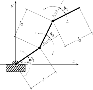
Figure 1. Schematic representation of a 3R planar robot.

As stated before, forward kinematics involves calculating the end-effector position, denoted as $p$, and orientation, represented by $\varphi$ (the angle relative to the world $x$-axis), based on the configuration of the robot, i.e., its joint angles. This is done using proper rigid body transformations (translations and rotations) that relate the world reference system to the end-effector coordinate system. Mathematically, the end-effector position and orientation of the robot is defined by the continuous functions:

(25) $$p=f(\theta_{1},\theta_{2},\theta_{3})\quad\text{and}\quad\varphi=g(\theta_{1},\theta_{2},\theta_{3})$$

The computation of $p$ and $\varphi$ is done using PGA, because as stated in 2.2, PGA is particularly well-suited to encode translations and rotations. Furthermore, as the forward kinematics problem does not involve the computation of spheres and circles, there is no necessity for the additional dimension and properties provided by CGA. The following code presents all the computation steps of the solution of the forward kinematics problem for an arbitrary 3R planar robot (where link lengths are also given as symbolic variables):

GA([2,0,1])                            % PGA 2D algebra initialization
Ψsyms angle_1 angle_2 angle_3 real      % joint angles
Ψsyms length_1 length_2 length_3 real   % link lengths
Ψ
ΨPoint2PGA=@(x,y)dual(x*e1 + y*e2 + e3) % function def.: point embedding for PGA2D
ΨPGA2Point=@(P) [P(e23),-P(e13)]ΨΨ       % function def.: point unembedding for PGA2D
ΨP0=Point2PGA(0,0)                      % point at the origin
Ψ
ΨD1=exp(length_1/2*e13);                % translation rotor of first link
ΨD2=exp(length_2/2*e13);                % translation rotor of second link
ΨD3=exp(length_3/2*e13);                % translation rotor of second link
Ψ
ΨR1=exp(-angle_1/2*e12);                % rotation rotor of first angle
ΨR2=exp(-angle_2/2*e12);                % rotation rotor of first angle
ΨR3=exp(-angle_3/2*e12);                % rotation rotor of first angle
Ψ
ΨR=R1*D1*R2*D2*R3*D3; ΨΨ                 % end-effector rotor
ΨP_ee=R*P0*~R;  ΨΨΨ                       % end-effector position
ΨP_ee_kin=simplify(PGA2Point(P_ee));    % end-effector symbolic explicit kinematics

which outputs the following solution:

P_ee_kin =
Ψ[length_2*cos(angle_1 + angle_2) + length_1*cos(angle_1) + length_3*cos(angle_1 +
Ψangle_2 + angle_3), length_2*sin(angle_1 + angle_2) + length_1*sin(angle_1) +
Ψlength_3*sin(angle_1 + angle_2 + angle_3)]

which coincides with the well-known expression for the forward kinematics of the 3R planar robot (Siciliano et al., 2008):

(26) $$p=\left(\begin{array}[]{c}x\\ y\end{array}\right)=\left(\begin{array}[]{c}\ell_{1}\cos(\theta_{1})+\ell_{2}\cos(\theta_{1}+\theta_{2})+\ell_{3}\cos(\theta_{1}+\theta_{2}+\theta_{3})\\ \ell_{1}\sin(\theta_{1})+\ell_{2}\sin(\theta_{1}+\theta_{2})+\ell_{3}\sin(\theta_{1}+\theta_{2}+\theta_{3})\end{array}\right)\quad\text{and}\quad\varphi=\theta_{1}+\theta_{2}+\theta_{3}$$

Therefore, the position and orientation of the robot’s end-effector can be represented by the rotor encoding its forward kinematics, i.e., the rotor encoding the geometric transformation that relates the world reference system to the end-effector coordinate system.

Finally, for every set of particular instances for the angles and lengths, the end-effector position and orientation can be determined via equation (26). To illustrate the capabilities of $\mathtt{SUGAR}$, a trajectory has been generated varying all the angles within a given range. Fig. 2 shows a sequence of plots where the end-effector of the $3$R planar robot arm (first joint in blue, second joint in red, and third joint in yellow) performs a trajectory (in purple), computed with equation (26) given these varying values for the angles.

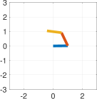
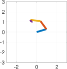
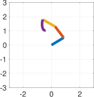
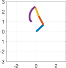
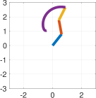
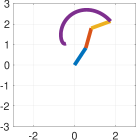
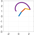
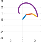
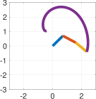
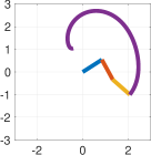
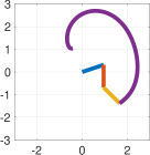
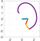
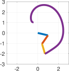
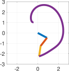
Figure 2. Trajectory for a 3R planar robot.

5.2. Inverse kinematics of a 6R robot

Consider a robot arm as the one depicted in Fig. 3. This is an example of one of the most typical industrial serial robots. The objective of this example is to illustrate the user-friendly capabilities of $\mathtt{SUGAR}$, as well as the manipulation of CGA-based solution strategies using $\mathtt{SUGAR}$. For that, the kinematic model and solution equations are taken directly from the source (Lavor et al., 2018) and implemented in $\mathtt{SUGAR}$.

In particular, the robot consists of three rigid links with lengths $d_{1}$, $a_{3}$, and $d_{4}$ (named according to the Denavit-Hartemberg convention, more details can be found in (Siciliano et al., 2008)), and six revolute joints connected in series. As in the case of 3R planar robots, this type of robot is known as a 6R robot. The last three joints act on the same point, contributing only to the orientation of the robot’s end-effector and not to its position. Similarly, the first three joints contribute to both the orientation and position of the robot’s end-effector. Therefore, to determine the spatial position of the end-effector of the robot, only the three first joints are needed. Its joint variables are three angles denoted as $\theta_{1}$, $\theta_{2}$, and $\theta_{3}$.

As stated before, inverse kinematics consists of finding the set all joint angles for a given position $p$ and orientation $\varphi$ of the robot’s end-effector. For this application example, and thanks to decoupling between position and orientation that the particular geometry of the robot allows, only the inverse position problem is considered. This means computing set of all values for $\theta_{1},\theta_{2}$ and $\theta_{3}$ or which the end-effector, in that configuration, is at the specified position $p$.

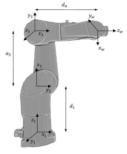
Figure 3. Schematic representation of a 6R robot.

Following the solution developed in (Lavor et al., 2018), if $p_{0}$ denotes the point placed at the origin of the world frame, then two intermediate points $p_{1}$ and $p_{2}$ are needed to be found. The steps are:

• The point $p_{0}$ is represented as a null vector of $\mathcal{G}_{4,1}$:

  (27) $$\bm{p}_{0}=H(p_{0})=\dfrac{1}{2}p_{0}^{2}n_{\infty}+n_{0}+p_{0}.$$

• The null vector $\bm{p}_{0}$ is translated in the direction $z_{1}$ of the world frame an amount equal to the first link length, i.e., $d_{1}$:

  (28) $$\bm{p}_{1}=T_{z_{1}}\bm{p}_{0}\widetilde{T}_{z_{1}},$$

  where $T_{z_{1}}=1-\frac{z_{1}\wedge n_{\infty}}{2}$.

• The inner representation of a sphere centered at $\bm{p}_{1}$ and with radius $a_{3}$ is computed:

  (29) $$\bm{s}_{1}^{\ast}=\bm{p}_{1}-\dfrac{1}{2}a_{3}^{2}e_{\infty}$$

• The inner representation of a sphere centered at $\bm{p}$ (the null vector representation of the given position $p$) and with radius $d_{4}$ is computed:

  (30) $$\bm{s}_{2}^{\ast}=\bm{p}-\dfrac{1}{2}d_{4}^{2}e_{\infty}$$

• The output representation of a plane passing through $\bm{p}_{0}$, $\bm{p}_{1}$ and $\bm{p}$ is computed:

  (31) $$\bm{\pi}=\bm{p}_{0}\wedge\bm{p}_{1}\wedge\bm{p}_{w}\wedge n_{\infty}$$

• The intersection of the plane and two spheres is computed:

  (32) $$B=(\bm{s}_{1}^{\ast}\wedge\bm{s}_{2}^{\ast}\wedge\bm{\pi}^{\ast})^{\ast},$$

  which is a bivector and, therefore, it represents a pair of points. In particular, $B=\bm{b}_{1}\wedge\bm{b}_{2}$ for some null vectors $\bm{b}_{1}$ and $\bm{b}_{2}$.

• Null vectors $\bm{b}_{1}$ and $\bm{b}_{2}$ are extracted from $B$:

  (33) $$\begin{split}\bm{b}_{1}&=-\widetilde{P}(B\cdot n_{\infty})P\\ \bm{b}_{2}&=P(B\cdot n_{\infty})\widetilde{P}\end{split}$$

  where $P$ denotes the projector operator defined as:

  (34) $$P=\dfrac{1}{2}\biggl{(}1+\dfrac{B}{\sqrt{B\widetilde{B}}}\biggr{)}$$

• Null vector $\bm{p}_{2}$ is equal to any of the recovered null vectors $\bm{b}_{i}$, $i=1,2$, i.e., there are two different solutions.

• For each value of $\bm{p}_{2}$, three auxiliary lines are computed:

  (35) $$\ell_{1} =\bm{p}_{0}\wedge\bm{p}_{1}\wedge n_{\infty}$$

  (36) $$\ell_{2} =\bm{p}_{1}\wedge\bm{p}_{2}\wedge n_{\infty}$$

  (37) $$\ell_{3} =\bm{p}_{2}\wedge\bm{p}\wedge n_{\infty}$$

• The joint angles are calculated:

  (38) $$\theta_{1} =\angle(x_{1},\pi)$$

  (39) $$\theta_{2} =\angle(\ell_{1},\ell_{2})$$

  (40) $$\theta_{3} =\angle(\ell_{2},\ell_{3})$$

  where $x_{1}$ is the $x$-axis of the world reference system.

The following code implements this solution in $\mathtt{SUGAR}$:

CGA(3)                                   % define 3D conformal geometric algebra
Ψd1 = 480;                                % define the Staübli robot link lengths
Ψa3= 425;
Ψd4 = 425;
Ψ
Ψq_d = [0.4375,0.8590,1.5040];            % desired configuration
Ψpos_d = [561.8479,262.7685,455.0104];    % associated desired position of the end-
Ψ% effector
ΨM_pos_d = pos_d(1)*e1+pos_d(2)*e2+pos_d(3)*e3 % multivector of the desired position
ΨPOS_D = push(M_pos_d);                        % push of the desired position
Ψ
ΨP0 = n0;                                      % compute p_0 (point at the origin)
ΨT1 = make_translation(d1,e3);                 % define the rotor for the translation
ΨP1 = T1.reverse*P0*T1;                        % compute p_1 (translation of p_1)
Ψ
Ψplane = P0.^P1.^POS_D.^ni;                    % plane passing by p_0, p_1 and pos_d
Ψ
Ψa = 0.5*(a3^2);                               % parameters from the link lengths
Ψd = 0.5*(d4^2);
Ψ
ΨS1 = P1 - a*ni;                               % sphere center = p_1 and radius = a3
ΨS2 = POS_D - d*ni;                            % sphere center = pos_d and radius = d4
Ψ
ΨC = S1.^S2;                                   % intersection of the spheres S1 and
Ψ% S2, results in a circle
ΨB = dual(plane).^clean(C);                    % intersection of the plane plane and
Ψ% circle C, results in a pair of points
ΨS1.plot()                                     % plot of all the geometric entitites
Ψhold on                                       % and their intersections
Ψ
ΨS2.plot()
Ψplane.normalize().plot()
ΨC.plot()
ΨB.plot();
Ψxlim([-1000,1000])
Ψylim([-1000,1000])
Ψhold off
Ψ
ΨP2_sol1 = B.info.P1;                          % extract first point P2 from B
ΨP2_sol2 = B.info.P2;                          % extract second point P2 from B
Ψ% continue with only one P2, the other
Ψ% is completely analagous
Ψnormal_plane = dual(plane).info.n;            % normal vector to plane plane
Ψnormal = normal_plane(e1+e2+e3);              % normal vector as GA vector
Ψx = [1,0,0];
Ψ
Ψ% first joint variable
Ψ
Ψq1 = acos(dot(normal,x)/(norm(x)*norm(normal)))-pi/2;
Ψ
Ψl1 = P0.^P1.^ni;                              % auxiliary line l1
Ψl2_sol1 = P1.^P2_sol1.^ni;                    % auxiliary line l2
Ψl3_sol1 = P2_sol1.^POS_D.^ni;                 % auxiliary line l3
Ψ
ΨL11 = l1*l1;                                  % module of line l1
ΨL11_scalar = L11(G0);                         % module as double
ΨL22_sol1 = l2_sol1*l2_sol1;                   % module of line l2
ΨL22_scalar_sol1 = L22_sol1(G0);               % module as double
ΨL33_sol1 = l3_sol1*l3_sol1;                   % module of line l3
ΨL33_scalar_sol1 = L33_sol1(G0);               % module as double
Ψ
ΨL12_sol1 = l2_sol1.*l1;                       % angle lines l1 and l2
ΨL12_scalar_sol1 = L12_sol1(G0);               % angle as double
Ψ
ΨL23_sol1 = l2_sol1.*l3_sol1;                  % angle lines l2 and l3
ΨL23_scalar_sol1 = L23_sol1(G0);               % angle as double
Ψ
Ψ% second and third joint variables
Ψ
Ψq2_sol1 = acos((L12_scalar_sol1)/(sqrt(L11_scalar)*sqrt(L22_scalar_sol1)));
Ψq3_sol1 = acos((L23_scalar_sol1)/(sqrt(L22_scalar_sol1)*sqrt(L33_scalar_sol1)));
Ψ
Ψq_proposed_sol1 = [q1,q2_sol1,q3_sol1]        % solution configuration

which outputs the following solution:

q_proposed_sol1 =
Ψ0.4375
Ψ0.8590
Ψ1.5040

that matches the input desired robot configuration. In addition, as demonstrated in the provided code, the translation of the theoretical solution presented by Lavor et al. (Lavor et al., 2018) can be easily implemented in $\mathtt{SUGAR}$ (in fact, it is completely straightforward). This, in turns, shows that the user-friendly part of SUGAR is justified. Furthermore, aside from the straightforward implementation of any computation step in GA, PGA and CGA, the CGA module incorporates a visualization tool that is essential to understand the complex geometric manipulations typically associated with mathematical and engineering applications using CGA. Fig. 4 depicts, as an illustrative example, the plot generated during the execution of the provided code.

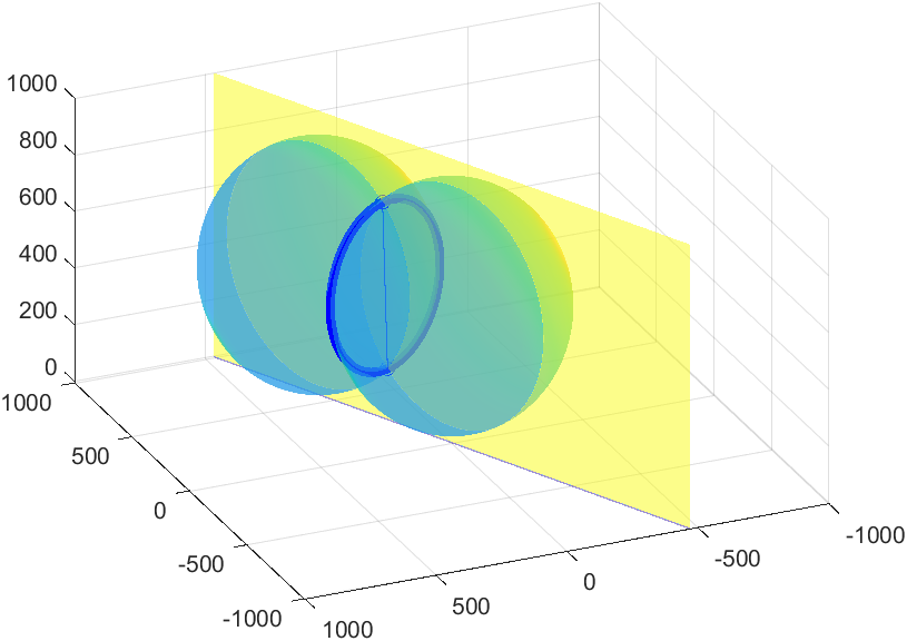
Figure 4. Geometric entities generated in the resolution of the inverse kinematics problem for the Stäubli robot and their intersections as generated in $\mathtt{SUGAR}$

5.3. 2-dimensional rigid body dynamics in PGA

This example shows how to obtain the dynamics of a uniform inertia hypercube (unit mass, unit inertia) using projective geometric algebra. For the sake of simplicity, a two-dimensional space is chosen, thus reducing the hypercube to a square. This example replicates the iconic simulation of the dynamics of an $n$-dimensional hypercube documented by Dorst and De Keninck (Dorst and Keninck, 2023), whose implementation with $\mathtt{ganja.js}$ is available at https://enki.ws/ganja.js/examples/coffeeshop.html#o0ZAc21EF.

The current dynamic state of a rigid body can be represented in PGA as a pair of multivectors $(M,B)$, where $M$ is the rotor representing its current position and orientation (as shown in subsection 5.1), while $B$ is the bivector representing its current linear and angular velocities. In particular, the rigid body dynamics are given by:

(41) $$\dot{M} =\frac{1}{2}MB$$

$$\dot{B} =(B^{*}\times B)^{-*}+F$$

where, as stated in section 2, $A^{*}$ denotes the dual of multivector $A$, $A^{-*}=(A^{\ast})^{\ast}$ denotes the double dual of multivector $A$, sometimes called the undual of $A$, and $\times$ denotes the geometric algebra commutator product, defined on vectors as:

(42) $$a\times b=\frac{1}{2}(ab-ba)$$

In addition, $F$ denotes the set of external forces and torques given by the gravity ($F_{g}$), Hooke’s law ($F_{H}$), and damping ($F_{d}$):

(43) $$F_{g}= -(\widetilde{M}9.8e_{23}M)^{*}$$

$$F_{H}= k(p_{b}\vee\widetilde{M}a_{w}M)$$

$$F_{d}= (-\alpha B)^{*}$$

where $p_{b}$ is a point in the rigid body, $a_{w}$ is the attachment point in the world frame, $k$ is the spring constant, $\vee$ is the regressive product (denoted in $\mathtt{SUGAR}$ by the command $\mathtt{and}$ or $\mathtt{\&}$), and $\alpha$ is the damping coefficient. Since $M$ is the rotor encoding the current position and orientation of the rigid body, the sandwich product $\widetilde{M}(\cdot)M$ express the element $(\cdot)$ from the world reference system to the coordinate system attached to the object. Note that the forces in (43) are expressed with respect to the rigid body’s coordinate system, and therefore, torques are also transformed using the sandwich product.

The dynamics of the rigid body are the solution of (41) subject to a given initial condition. The following code obtains the symbolic dynamics of the considered square:

GA([2,0,1])                                  % define 2D Projective Geometric Algebra
ΨPoint2PGA=@(x,y)dual(x*e1 + y*e2 + e3);      % transforms 2D point to PGA
ΨPGA2Point=@(P) [P(e23),-P(e13)]Ψ             % transforms PGApoint to 2D
Ψpoints_list = [Point2PGA(-0.75,-0.75),...    % definition of square vertices
ΨPoint2PGA( 0.75,-0.75),...
ΨPoint2PGA( 0.75, 0.75),...
ΨPoint2PGA(-0.75, 0.75)]
Ψattaching_index=4;                           % attached point
Ψattached = points_list(attaching_index);
Ψsyms x0 y0;                                  % attaching point position
Ψx_attach=x0;y_attach=y0;                     % can be numeric or symbolic
Ψattach = Point2PGA(x_attach,y_attach);
Ψsyms k a                                     % external forces constants
ΨF=@(S)dual(S(1).reverse*(-9.8*e23)*S(1))...  % gravity (negative direction, downwards)
Ψ-k*(attached&(S(1).reverse*attach*S(1)))...% Hooke (from & to, obiously negative)
Ψ+dual((-a * S(2))) ;                       % damping (oposite to speed)
Ψ
ΨState_derivative=@(S)[0.5*S(1)*S(2), ...     % dynamics
Ψ(F(S)+0.5*(S(2).dual*S(2)-S(2)*S(2).dual)).grade(2)]
Ψsyms R Dx Dy Rs Dxs Dys real                 % rotation, displacements and speeds
Ψ% Symbolic initial state
ΨM0=exp(1/2*(Dx*e13+Dy*e23+R*e12));           % position and orientation initial state
ΨB0=Dxs*e13+Dys*e23+Rs*e12.                   % linear and angular velocities
Ψstate  = [M0, B0];
ΨSD=State_derivative(state).’;                % symbolic dynamics

which returns the desired dynamics in terms of the time-derivative of the states, that is, the time-derivative of multivectors $M$ and $B$:

(44) $$\left(\begin{array}[]{c}\\ \\ \dot{M}\\ \\ \\ \\ \\ \dot{B}\\ \\ \\ \end{array}\right)=\left(\begin{array}[]{c}\left(-\frac{\mathrm{Rs}\,\sin\left(\frac{R}{2}\right)}{2}\right)e_{0}\\ +\left(\frac{\mathrm{Rs}\,\cos\left(\frac{R}{2}\right)}{2}\right)e_{12}\\ +\left(\frac{\mathrm{Dxs}\,\cos\left(\frac{R}{2}\right)}{2}+\frac{\mathrm{Dys}\,\sin\left(\frac{R}{2}\right)}{2}-\frac{\mathrm{Dy}\,\mathrm{Rs}\,\sin\left(\frac{R}{2}\right)}{2\,R}\right)e_{13}\\ +\left(\frac{\mathrm{Dys}\,\cos\left(\frac{R}{2}\right)}{2}-\frac{\mathrm{Dxs}\,\sin\left(\frac{R}{2}\right)}{2}+\frac{\mathrm{Dx}\,\mathrm{Rs}\,\sin\left(\frac{R}{2}\right)}{2\,R}\right)e_{23}\\ \left(-\frac{\mathrm{Dx}\,k-\mathrm{Dy}\,k+2\,R\,\mathrm{Rs}\,a-\mathrm{Dx}\,k\,\cos\left(R\right)+\mathrm{Dy}\,k\,\cos\left(R\right)+\mathrm{Dx}\,k\,\sin\left(R\right)+\mathrm{Dy}\,k\,\sin\left(R\right)-R\,k\,x_{0}\,\cos\left(R\right)-R\,k\,y_{0}\,\cos\left(R\right)-R\,k\,x_{0}\,\sin\left(R\right)+R\,k\,y_{0}\,\sin\left(R\right)}{2\,R}\right)e_{12}\\ +\left(-\frac{10\,\mathrm{Dys}\,R\,\mathrm{Rs}-5\,R\,k-98\,R\,\sin\left(R\right)-10\,\mathrm{Dy}\,k+10\,\mathrm{Dxs}\,R\,a+10\,\mathrm{Dy}\,k\,\cos\left(R\right)+10\,\mathrm{Dx}\,k\,\sin\left(R\right)-10\,R\,k\,x_{0}\,\cos\left(R\right)+10\,R\,k\,y_{0}\,\sin\left(R\right)}{10\,R}\right)e_{13}\\ +\left(-\frac{10\,\mathrm{Dx}\,k+5\,R\,k+98\,R\,\cos\left(R\right)-10\,\mathrm{Dxs}\,R\,\mathrm{Rs}+10\,\mathrm{Dys}\,R\,a-10\,\mathrm{Dx}\,k\,\cos\left(R\right)+10\,\mathrm{Dy}\,k\,\sin\left(R\right)-10\,R\,k\,y_{0}\,\cos\left(R\right)-10\,R\,k\,x_{0}\,\sin\left(R\right)}{10\,R}\right)e_{23}\\ \end{array}\right)$$

where $R$ is the rotational displacement of the rigid body, $Dx,Dy$ are the lineal displacements of the rigid body, and $Rs,Dxs$ and $Dys$ are the angular and linear velocities components of the rigid body.

Given a set of initial values for the position and layout of the square, its dynamics can be obtained via equation (44). For instance, Fig. 5 displays a sequence of plots where the square is assigned an initial condition that initiates the movement illustrated in the plots.

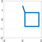
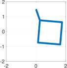
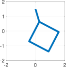
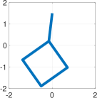
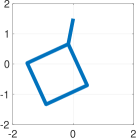
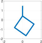
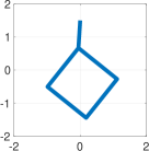
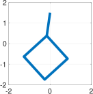
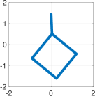
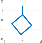
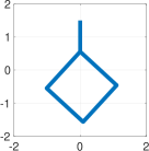
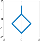
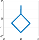
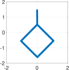
Figure 5. Sequence of a square body dynamics.

5.4. Power systems analysis

This example illustrates the capability of $\mathtt{SUGAR}$ for operating with matrices of multivectors, and in particular, for calculating the inverse of a matrix of multivectors. Such operation, which in general is rarely found in other existing computational libraries (or even inexistent for symbolic computing), can be exploited for example when working with electrical systems modelled using a GA approach (Velasco et al., 2023).

Unbalanced three-phase electrical systems can be represented using GA, where voltages and currents are multivectors and are related by geometric impedances with the form

(45) $$z(s)=z_{\mathrm{av}}(s)e_{0}+z_{\mathrm{unI}}(s)e_{1}+z_{\mathrm{unR}}(s)e_{2}$$

where $z_{\mathrm{av}}(s),z_{\mathrm{unI}}(s)$ and $z_{\mathrm{unR}}(s)$ are transfer functions. In case of balanced impedances $z_{\mathrm{unI}}(s)=z_{\mathrm{unR}}(s)=0$. See more details in (Dòria-Cerezo et al., 2024).

Figure 6. A three-phase unbalanced electrical power network.

Figure 6 shows the equivalent circuit of a three-phase electrical power grid with an ideal power source (slack), three lines connecting nodes 1, 2, and 3, and two consumers at nodes 2 and 3. The geometric impedances $z_{12}(s),z_{13}(s),z_{23}(s)$ represent the dynamics and dissipation of the connection lines, $z_{L2}(s),z_{L3}(s)$ represent the electrical loads of consumers, and $v_{s}$ is the multivector representing the power source voltage.

The nodal analysis is one of the most used approaches for the analysis of power networks (Dimo, 1975) and allows us to find the voltages at all the nodes of the circuit by solving a matrix equation. The method is based on creating the admittance matrix, $Y$, of the circuit, where the matrix elements are composed of the circuit admittances defined as

(46) $$y(s)=z^{-1}(s).$$

For the example in Figure 6, the matrix equation results in

(47) $$\underbrace{\begin{pmatrix}y_{12}(s)+y_{13}(s)&-y_{12}(s)&-y_{13}(s)&1\\ -y_{12}(s)&y_{12}(s)+y_{23}(s)+y_{L2}(s)&-y_{23}(s)&0\\ -y_{13}(s)&-y_{23}(s)&y_{13}(s)+y_{13}(s)+y_{L3}(s)&0\\ 1&0&0&0\end{pmatrix}}_{Y}\begin{pmatrix}v_{1}\\ v_{2}\\ v_{3}\\ i_{s}\end{pmatrix}=\begin{pmatrix}0\\ 0\\ 0\\ v_{s}\end{pmatrix}$$

where the system unknowns are the node voltages, $v_{1},v_{2},v_{3}$, and the current of the power source, $i_{s}$.

Consider the power network described in a per-unit (adimensional) system, with $v_{s}=v_{\alpha}(t)e_{0}+v_{\beta}(t)e_{1}+v_{\alpha}(t)e_{2}+v_{\beta}(t)e_{12}$ and the line and load geometric impedances with values

(48) $$z_{12}(s) =(0.02s+0.01)e_{0}$$

(49) $$z_{13}(s) =(0.04s+0.02)e_{0}$$

(50) $$z_{23}(s) =(0.02s+0.01)e_{0}$$

(51) $$z_{L2}(s) =0.5e_{0}-0.0289e_{1}+0.05e_{2}$$

(52) $$z_{L3}(s) =0.4e_{0}-0.11559e_{1}-0.1e_{2}$$

with the aim of finding the voltage dynamics in node 2.

The solution of (47) can be easily done in $\mathtt{SUGAR}$:

syms s;                                          % symbolic Laplace variable
Ψsyms va vb;                                      % symbolic voltage variables
ΨGA([2 0 0]);                                     % GA definition
Ψ
Ψr12=0.01; l12=0.02; Ψ                            % line 12 parameters
Ψr13=0.02; l13=0.04; Ψ                            % line 13 parameters
Ψr23=0.01; l23=0.02; Ψ                            % line 23 parameters
ΨR2av=0.5; R2unI=-0.0289; R2unR=0.05;  Ψ          % load 2 parameters
ΨR3av=0.4; R3unI=-0.1155; R3unR=-0.1;  Ψ          % load 3 parameters
Ψvs=va*e0+vb*e1+va*e2+vb*e12;                     % slack voltage
Ψ
Ψz12=(r12+l12*s)*e0;                              % line 12 impedance definition
Ψz13=(r13+l13*s)*e0;                              % line 13 impedance definition
Ψz23=(r23+l23*s)*e0;                              % line 21 impedance definition
ΨzL2=R2av*e0+R2unI*e1+R2unR*e2;                   % load 2 impedance definition
ΨzL3=R3av*e0+R3unI*e1+R3unR*e2;                   % load 3 impedance definition
Ψ
Ψy12=clean(inv(z12));                             % admittance calculation
Ψy13=clean(inv(z13));                             % admittance calculation
Ψy23=clean(inv(z23));                             % admittance calculation
ΨyL2=clean(inv(zL2));                             % admittance calculation
ΨyL3=clean(inv(zL3));                             % admittance calculation
ΨY=[y12+y13 -y12 -y13 1*e0;                       % admittance matrix
Ψ-y12 y12+y23+yL2 -y23 0*e0;
Ψ-y13 -y23 y13+y23+yL3 0*e0;
Ψ1*e0 0*e0 0*e0 0*e0];
Ψ
Ψx=inv(Y)*[0*e0;0*e0;0*e0;vs]                     % solving the system
Ψ
Ψv2=x(2);                                         % MV voltage at node 2
Ψ[Nv2e0,Dv2e0]=numden(v2(1))                      % polynomials of TF with e0
Ψ[Nv2e1,Dv2e1]=numden(v2(2))                      % polynomials of TF with e1
Ψ[Nv2e2,Dv2e2]=numden(v2(3))                      % polynomials of TF with e2
Ψ[Nv2e12,Dv2e12]=numden(v2(4))                    % polynomials of TF with e12

providing the polynomials of the transfer functions in the multivector $v_{2}$:

Nv2e0=14595547*va-62633*vb+1596858*s*va-126698*s*vb+50148*s^2*va+440*s^3*va...
Ψ-2876*s^2*vb-24*s^3*vb
ΨDv2e0=16*s^4+2592*s^3+136080*s^2+2552384*s+15052095
Ψ
ΨNv2e1=14651277*vb-62553*va-126378*s*va+1706478*s*vb-2556*s^2*va-24*s^3*va...
Ψ+46428*s^2*vb+360*s^3*vb
ΨDv2e1=16*s^4+2592*s^3+136080*s^2+2552384*s+15052095
Ψ
ΨNv2e2=14595547*va-62633*vb+1596858*s*va-126698*s*vb+50148*s^2*va+440*s^3*va...
Ψ-2876*s^2*vb-24*s^3*vb
ΨDv2e2=16*s^4+2592*s^3+136080*s^2+2552384*s+15052095
Ψ
ΨNv2e12=14651277*vb-62553*va-126378*s*va+1706478*s*vb-2556*s^2*va-24*s^3*va...
Ψ+46428*s^2*vb+360*s^3*vb
ΨDv2e12=16*s^4+2592*s^3+136080*s^2+2552384*s+15052095

6. Conclusions

This work has presented $\mathtt{SUGAR}$, a Matlab toolbox for symbolic and numerical computing with geometric algebras. It complements existing GA software by offering the capacity to perform symbolic computations and providing a mathematical and engineering-oriented design to facilitate its applicability in different disciplines in a user-friendly manner. To this end, apart from introducing the main building blocks and functions of $\mathtt{SUGAR}$, the article provides several examples ranging from standard robotics to iconic rigid body dynamics simulations, and even covers new applications like the use of geometric algebra for the modeling and analysis of power electronics.

As future work, some interesting remarks have arisen from the different tests performed with $\mathtt{SUGAR}$. In particular, $\mathtt{SUGAR}$ has opened the door to the development of closed-form formulas for the inverse of a multivector, the inverse of a matrix of multivectors, and even the exponential of a multivector, which have not been fully addressed in the literature. In addition, other less-used functions like $\log$, $\sin$, $\cos$ can also benefit from the closed-form formulas that can be obtained with $\mathtt{SUGAR}$.

References

- (1)
- Ablamowicz and Fauser (2005) Rafal Ablamowicz and Bertfried Fauser. 2005. Mathematics of CLIFFORD - A Maple package for Clifford and Grassmann algebras. Advances in Applied Clifford Algebras 15 (01 2005), 157–181. https://doi.org/10.1007/s00006-005-0009-9
- Antanovskii (2014) L.K. Antanovskii. 2014. Implementation of Geometric Algebra in MATLAB with Applications. Technical Report. DSTO–TR–3021 Weapons and Combat Systems Division, Defence Science and Technology Organisation, Dept. of Defense, Australian Government, https://apps.dtic.mil/sti/pdfs/ADA615302.pdf.
- Awad Eid (2016) Ahmad Hosney Awad Eid. 2016. Optimized Automatic Code Generation for Geometric Algebra Based Algorithms with Ray Tracing Application. arXiv:1607.04767
- Bayro-Corrochano (2020) Eduardo Bayro-Corrochano. 2020. Geometric Algebra Applications Vol. II: Robot Modelling and Control. Springer. https://doi.org/10.1007/978-3-030-34978-3
- Bayro-Corrochano (2021) Eduardo Bayro-Corrochano. 2021. A Survey on Quaternion Algebra and Geometric Algebra Applications in Engineering and Computer Science 1995–2020. IEEE Access 9 (2021), 104326–104355. https://doi.org/10.1109/ACCESS.2021.3097756
- Bayro-Corrochano et al. (2022) Eduardo Bayro-Corrochano, Jesus Medrano-Hermosillo, Guillermo Osuna-González, and Ulises Uriostegui-Legorreta. 2022. Newton–Euler modeling and Hamiltonians for robot control in the geometric algebra. Robotica 40, 11 (2022), 4031–4055. https://doi.org/10.1017/S0263574722000741
- Bromborsky and team (2014) Alan Bromborsky and GAlgebra team. 2014. GAlgebra. Army Research Lab. https://github.com/pygae/galgebra
- Calvet (2017) Ramon Calvet. 2017. On Matrix Representations of Geometric (Clifford) Algebras. Journal of Geometry and Symmetry in Physics 43 (01 2017), 1–36. https://doi.org/10.7546/jgsp-43-2017-1-36
- Chappell et al. (2014) James M. Chappell, Samuel P. Drake, Cameron L. Seidel, Lachlan J. Gunn, Azhar Iqbal, Andrew Allison, and Derek Abbott. 2014. Geometric Algebra for Electrical and Electronic Engineers. Proc. IEEE 102, 9 (2014), 1340–1363. https://doi.org/10.1109/JPROC.2014.2339299
- Colapinto (2011) Pablo Colapinto. 2011. Versor: Spatial Computing with Conformal Geometric Algebra. Master’s thesis. University of California Santa Barbara, http://versor.mat.ucsb.edu. http://versor.mat.ucsb.edu
- Dargys and Acus (2021) Adolfas Dargys and Arturas Acus. 2021. Exponentials of general multivector (MV) in 3D Clifford algebras. arXiv:2104.01905
- De Keninck (2017) Steven De Keninck. 2017. ganja.js. University of Amsterdam. https://github.com/enkimute/ganja.js
- Dimo (1975) Paul Dimo. 1975. Nodal analysis of power systems. Abacus Press.
- Doran and Lasenby (2003) C. Doran and A. Lasenby. 2003. Geometric Algebra for Physicists. Cambridge University Press.
- Dorst and Keninck (2022) Leo Dorst and Steven De Keninck. 2022. Guided tour to the plane-based geometric algebra PGA. https://bivector.net/PGA4CS.html.
- Dorst and Keninck (2023) Leo Dorst and Steven De Keninck. 2023. May the Forque be with you, dynamics in PGA. https://bivector.net/PGADYN.html.
- Dòria-Cerezo et al. (2024) A. Dòria-Cerezo, M. Velasco, I. Zaplana, and P. Martí. 2024. The Ohm’s Law for (non-symmetric) three-phase three-wire electrical circuits: from a complex-valued to a geometric algebra approach. Springer.
- Hestenes (2001) David Hestenes. 2001. Old Wine in New Bottles: A New Algebraic Framework for Computational Geometry. In Geometric Algebra with Applications in Science and Engineering, Eduardo Bayro Corrochano and Garret Sobczyk (Eds.). Birkhäuser Boston, 3–17.
- Hestenes and Sobczyk (1984) David Hestenes and Garret Sobczyk. 1984. Clifford algebra to geometric calculus : a unified language for mathematics and physics. D. Reidel ; Distributed in the U.S.A. and Canada by Kluwer Academic Publishers, Dordrecht; Boston; Hingham, MA, U.S.A.
- Hitzer et al. (2013) Eckhard Hitzer, Tohru Nitta, and Yasuaki Kuroe. 2013. Applications of Clifford’s Geometric Algebra. Advances in Applied Clifford Algebras 23, 2 (2013), 377–404. https://doi.org/10.1007/s00006-013-0378-4
- Hitzer and Sangwine (2017) Eckhard Hitzer and Stephen Sangwine. 2017. Multivector and multivector matrix inverses in real Clifford algebras. Appl. Math. Comput. 311 (2017), 375–389. https://doi.org/10.1016/j.amc.2017.05.027
- Lavor et al. (2018) C. Lavor, S. Xambó-Descamps, and I. Zaplana. 2018. A Geometric Algebra Invitation to Space-Time Physics, Robotics and Molecular Geometry. SpringerBriefs in Mathematics, Springer Cham.
- Lounesto et al. (1987) Pertti Lounesto, R. Mikkola, and V. Vierros. 1987. CLICAL user manual: complex number, vector space and Clifford algebra calculator for MS-DOS personal computers. Technical Report. Helsinki University of Technology, Finland, https://users.aalto.fi/~ppuska/mirror/Lounesto/CLICAL.htm.
- Löw and Calinon (2023) Tobias Löw and Sylvain Calinon. 2023. Geometric Algebra for Optimal Control With Applications in Manipulation Tasks. IEEE Transactions on Robotics 39, 5 (2023), 3586–3600. https://doi.org/10.1109/TRO.2023.3277282
- Mann et al. (1999) S. Mann, L. Dorst, and T. Bouma. 1999. The making of a geometric algebra package in Matlab. Technical Report. University of Waterloo, Canada, https://cs.uwaterloo.ca/research/tr/1999/27/CS-99-27.pdf.
- Ortiz-Duran and Aragon (2017) E. Alejandra Ortiz-Duran and Jose L. Aragon. 2017. CGAlgebra: a Mathematica package for conformal geometric algebra. v.2.0. arXiv:1711.02513
- Prodanov and Toth (2017) Dimiter Prodanov and V. Toth. 2017. Sparse Representations of Clifford and Tensor Algebras in Maxima. Advances in Applied Clifford Algebras 27 (2017), 661–683. https://doi.org/10.1007/s00006-016-0682-x
- Roelfs and Keninck (2023) Martin Roelfs and Steven De Keninck. 2023. Graded Symmetry Groups: Plane and Simple. Advances in Applied Clifford Algebras 30, 33 (2023), 1–41. https://doi.org/10.1007/s00006-023-01269-9
- Sangwine and Le Bihan (2005) Steve Sangwine and Nicolas Le Bihan. 2005. Quaternion and octonion toolbox for Matlab. Grenoble-INP and Université de Grenoble-Alpes. https://qtfm.sourceforge.io/
- Sangwine and Hitzer (2016) Stephen J. Sangwine and Eckhard Hitzer. 2016. Clifford Multivector Toolbox (for MATLAB). Advances in Applied Clifford Algebras 27, 1 (apr 2016), 539–558. https://doi.org/10.1007/s00006-016-0666-x
- Siciliano et al. (2008) B. Siciliano, L. Sciavicco, L. Villani, and G. Oriolo. 2008. Robotics: Modelling, Planning and Control. Springer Publishing Company.
- Velasco (2023) Manel Velasco. 2023. Symbolic and User-friendly Geometric Algebra Routines (SUGAR). Universitat Politècnica de Catalunya (UPC). https://github.com/distributed-control-systems/SUGAR
- Velasco et al. (2023) Manel Velasco, Isiah Zaplana, Arnau Dòria-Cerezo, Josué Duarte, and Pau Martí. 2023. Introducing Modelling, Analysis and Control of Three-Phase Electrical Systems Using Geometric Algebra. arXiv:2312.01345
- Zaplana et al. (2022a) Isiah Zaplana, Hugo Hadfield, and Joan Lasenby. 2022a. Closed-form solutions for the inverse kinematics of serial robots using conformal geometric algebra. Mechanism and Machine Theory 173 (2022), 104835. https://doi.org/10.1016/j.mechmachtheory.2022.104835
- Zaplana et al. (2022b) Isiah Zaplana, Hugo Hadfield, and Joan Lasenby. 2022b. Singularities of Serial Robots: Identification and Distance Computation Using Geometric Algebra. Mathematics 10, 12 (2022), 2068. https://doi.org/10.3390/math10122068