Improving the Optimization in Model Predictive Controllers: Scheduling Large Groups of Electric Vehicles

Abstract

In parking lots with large groups of electric vehicles (EVs), charging has to happen in a coordinated manner, among others, due to the high load per vehicle and the limited capacity of the electricity grid. To achieve such coordination, model predictive control can be applied, thereby repeatedly solving an optimization problem. Due to its repetitive nature and its dependency on the time granularity, optimization has to be (computationally) efficient.

The work presented here focuses on that optimization subroutine, its computational efficiency and how to speed up the optimization for large groups of EVs. In particular, we adapt Focs, an algorithm that can solve the underlying optimization problem, to better suit the repetitive set-up of model predictive control by adding a pre-mature stop feature. Based on real-world data, we empirically show that the added feature speeds up the median computation time for 1-minute granularity by up to 44%. Furthermore, since Focs is an algorithm that uses maximum flow methods as a subroutine, the impact of choosing various maximum flow methods on the runtime is investigated. Finally, we compare Focs to a commercially available solver, concluding that Focs outperforms the state-of-the-art when making a full-day schedule for large groups of EVs.

I Introduction

With the on-going transition to electric mobility, the number of electric vehicles (EVs) in the Netherlands is increasing rapidly [1]. Especially near-work locations have been found to be good locations to charge large groups of EVs, partially due to the long stays [2] and the potential availability of solar energy [3]. However, due to limited grid capacity [4], high synchronicity [5] and possible temporal mismatches with said solar energy production [6], charging has to occur in a coordinated manner. For successful coordination, a controller needs information on the charging sessions, for example the (expected) energy demand and departure time of an EV in the parking lot. In practice, the EVs currently do not communicate such information [7]. Therefore, next to the sheer amount of charge required per vehicle, the biggest challenge in managing the charging processes of the EVs is the absence of information.

To bridge this information gap, model predictive control (Mpc) can be applied (e.g., [8]). Based on the information available at the current point in time and an underlying system model, Mpc generates and solves a suitable offline optimization problem and an (in time) initial portion of this solution is realized. This process is repeated frequently over the given time horizon. Specifically to solve this offline problem, the Flow-Based Offline Charging Scheduler (Focs) has been developed [9]. Focs is a polynomial time algorithm which in theory has a complexity of $\mathcal{O}(n^{2}\mu)$, where $n$ is the number of EVs to be charged and $\mu$ is the complexity of the maximum flow algorithm embedded in Focs.

Notably, research has shown that for some algorithms theoretical and empirical runtime do not align. For example, the simplex algorithm, while theoretically exponential in runtime, performs well in practice. The other way around, Ellipsoid methods for linear programs are known to be polynomial on paper, while performing poorly in practice. This motivates us to investigate the empirical runtime of the novel algorithm Focs based on real world EV data.

The main contributions of the work presented here are:

• Introduction and validation of a pre-mature stop feature that increases computational efficiency in model predictive controllers using Focs.

• Extensive comparative runtime analysis of Focs, and its validation using real world EV charging data.

The remainder of the paper is organized as follows. Section II discusses the mathematical model of the considered EV scheduling problem (Section II-A), briefly introduces Focs (Section II-B) and proposes a pre-mature stop feature for Focs (Section II-C) expected to increase its efficiency for Mpc applications. Then, Section III specifies the experimental setup and gives some information on the implementation of the used algorithms. Furthermore, the section describes the real world data set used for the experiments (Section III-C). Section IV presents the experimental results, followed by a discussion in Section V and a conclusion in Section VI.

II EV scheduling problem and algorithms

In this section, we describe the considered EV scheduling problem in terms of notation, constraints and considered objective function. Furthermore, we briefly introduce Focs, an algorithm that can be used to determine an optimal solution for said problem. For more details on Focs, we refer to [9].

II-A Problem definition

We consider jobs $1,...,n$, where each job $j$ corresponds to a pending charging session (or EV) with associated energy requirement $e_{j}$, arrival time $a_{j}$, departure time $d_{j}$ and job-specific charging power limit $p_{j}^{\max}$. We denote the set of all jobs by $[n]$. We consider a problem instance feasible if

$$e_{j}\leq p_{j}^{\max}(d_{j}-a_{j})\hskip 10.0pt\forall j\in[n].$$

Moreover, we discretize the time horizon $[\min_{j}a_{j},\max_{j}d_{j}]$ into atomic intervals by using all arrival and departure times of EVs as breakpoints. The resulting (ordered) sequence of breakpoints we denote as $t_{1},\dots,t_{m+1}$, resulting in $m\leq 2n-1$ atomic intervals $I_{i}=[t_{i},t_{i+1}]$ for $i=1,...,m$.

To relate jobs to atomic intervals, we denote by $J(i)$ the jobs that are available in interval $I_{i}$, i.e.,

$$J(i)=\{j|(a_{j}\leq t_{i})\land(t_{i+1}\leq d_{j})\}.$$

Similarly, $J^{-1}(j)$ is defined as the set of indices $i$ of the intervals $I_{i}$ where $j$ is available. Finally, as atomic intervals are in general not unit-sized, we introduce maximum energy limits $e_{i,j}^{\max}=p_{j}^{\max}(t_{i+1}-t_{i})$ per job $j$ and interval $I_{i}$.

As decision variables, let $e_{i,j}$ be the energy that EV $j$ charges in $I_{i}$. Note that preemption is allowed, meaning the charging can be suspended for a few intervals to be continued at a later interval. In this work, we do not consider V2G, implying that $e_{i,j}\geq 0$.

Summarizing, the EV model is constrained by

$$\sum_{i\in J^{-1}(j)}e_{i,j} \geq e_{j} \forall j\in[n]$$ (1a)

$$e_{i,j} \geq 0 \forall j\in[n],i\in J^{-1}(j)\hskip 3.0pt$$ (1b)

$$e_{i,j} \leq e_{i,j}^{\max} \forall j\in[n],i\in J^{-1}(j).$$ (1c)

From a grid perspective, the aggregated power level resulting from an EV schedule is of interest. For a given schedule, the average aggregated power level $p_{i}$ in atomic interval $I_{i}$ is given by

$$p_{i}=\frac{\sum_{j\in J(i)}e_{i,j}}{t_{i+1}-t_{i}}.$$

The two most frequently considered objectives for the overall grid usage are the $\ell_{\infty}$ and $\ell_{2}$-norms of the aggregated power. Focs was developed for minimization of objective functions

$$F\left(p_{1},\dots,p_{m}\right)$$ (2)

that are convex, differentiable and for which increasing any value $p_{i}$ increases the value of the objective function. The complexity of Focs is independent on the exact form of the objective function. In this work, we specifically consider the square of the $\ell_{2}$-norm given by

$$F\left(p_{1},\dots,p_{m}\right)=\sum_{i=1}^{m}L_{i}\cdot\left(p_{i}^{2}\right)$$ (3)

where $L_{i}$ is a normalization term to account for the length of the interval.

II-B The general working of Focs

Focs is a recursive algorithm that finds an optimal solution to the problem described above. To this end, it makes use of various properties of optimal solutions to this problem. First, any optimal aggregated power profile that minimizes an objective function (2) is a step function in the sense that within each atomic interval, the aggregated power is constant. Based on this, Focs iteratively identifies a critical interval where the highest speed is needed, determines the minimum speed for this interval, and fixes the schedule for this interval, ultimately minimizing the maximum peak. The selected critical interval and the charge provided in that interval are then removed from the problem instance.

To determine the critical intervals, Focs computes multiple iterations of maximum flows. Figure 1 depicts the basic structure of the considered flow network. Here, at each iteration, Focs adapts the capacities of edges adjacent to sink node $t$. The iterations until a critical interval is identified, form a round $r$. The edge capacities $g_{r,k}:\{I_{i}|i\in[m]\}\rightarrow\mathbb{R}_{\geq 0}$ in round $r$ and iteration $k$ represent a fill-level that is increased over the iterations until critical interval(s) are found.

Figure 1: Schematic of flow network structure of EV charging schedule.

II-C Adapting Focs for model predictive control

Focs was developed to determine the optimal solution of the offline EV scheduling problem described in Section II-A. To this end, it solves the instance over the entire planning horizon. However, for Mpc, often only the next (few) time intervals and their control actions are of interest. Based on this, we propose an adaptation to Focs. For convenience, we assume in the following that only the first time interval is of interest. The proposed concept extends naturally to include the first few intervals.

$j$	$a_{j}$	$d_{j}$	$e_{j}$	$p_{j}^{\max}$
1	0	2	4	2
2	1	3	2	1

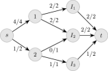
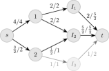
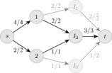
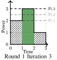
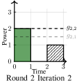
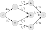
Figure 2: Intermediate states of Focs with pre-mature stop for an example instance, tracked over rounds and iterations.

Focs recursively identifies intervals that require the highest aggregated power in an optimal schedule (so-called critical intervals), determines the partial schedule corresponding to that interval, and repeats this with the remaining problem instance. In particular, each of those recursion steps fixes a part of the optimal schedule. Therefore, if we are only interested in the schedule of the first interval, we can pre-maturely terminate Focs once the schedule for that interval was found, without losing any information on the first interval.

We illustrate this concept in Figure 2 for an instance with two EVs and three intervals. The annotations at the edges of the flow network are of the form $x/y$, where $x$ is the flow going through the edge, and $y$ is the edge capacity. Moreover, the green shaded blocks are the identified critical intervals. Those are fixed, and in the last step combined into the algorithm output. After finding the schedule for the first interval (i.e., when we find the green block for the first interval in the fifth step in Figure 2), we terminate the algorithm. Note that even though the schedule for the third interval has not yet been found and thereby the returned schedule (last power profile in Figure 2) is not feasible considering the entire problem instance, there exists an optimal schedule that complements the found partial solution. In particular, the aggregated power in the first interval is optimal. This follows by optimality of Focs, and the following lemmas paraphrased from [9].

Lemma 1

(Lemma 2 in [9]) If a critical interval $I_{i}$ and its aggregated power are found, and if there is at least one interval $I_{i^{\prime}}$ left that at that point has not yet been scheduled, then no scheduled charging work can feasibly be moved from $I_{i}$ to $I_{i^{\prime}}$ for any such $I_{i^{\prime}}$.

Lemma 2

(Lemma 3 in [9]) The aggregated power of the subsequently identified (sets of) critical intervals by Focs is strictly decreasing. In particular, if Focs fixes the schedule for $I_{i}$ before that of $I_{i^{\prime}}$, then

$$p_{i}>p_{i^{\prime}}$$

in the optimal solution.

For the precise formulation and proof of the lemmas, we refer the reader to [9].

Notably, for EV parking lots near office locations, the optimal schedule over a day typically resembles a concave curve. The pre-mature stop feature we propose here terminates the algorithm once the first interval has been scheduled, where intervals are scheduled by order of their aggregated power in the optimal solution. Therefore, the time of day at which we apply the pre-mature stop feature impacts its effectiveness. In particular for an office parking lot, we expect the greatest reduction in computation time with pre-mature stop compared to the unrestricted Focs to be around noon. In the following, we refer to the implementation of Focs with pre-mature stop as Focs-pm.

III Methods

In this section, we provide some details on the implementation of the three tested optimization models (Quadratic program in Gurobi (QP), Focs and Focs with pre-mature stop (Focs-pm)), after which we describe the experimental setup and real-world data set used.

III-A QP implementation

Based on the problem constraints (1) and the quadratic objective function (3), we use the commercial solver Gurobi [10] to solve this problem. Gurobi is used for comparison with state-of-the art solvers. Note that while Focs leads to optimal solutions also for more general objective functions, for practical reasons we compare its runtime to a Gurobi model and for that we restrict us to a quadratic objective function.

III-B Focs implementation

The Focs implementation used for the empirical runtime analysis of Focs has been developed specifically as a proof of concept for this paper. The code is written in python, heavily relying on the networkx package [11]. This package is chosen for its user friendly flow models, and because various maximum flow algorithms are readily available within the package. An overview of the considered algorithms is provided in Table I.

TABLE I: Complexity table for four maximum flow algorithms. Here, $N$, $M$ and $U$ are respectively the number of nodes, edges and the maximum capacity in a given flow network.

Max flow algorithm	Complexity [12]	Networkx complexity	Complexity on Focs network
shortest_augmenting_path()	$\mathcal{O}(NMU)$	$\mathcal{O}(N^{2}M)$	$\mathcal{O}(n^{4})$
edmonds_karp()	$\mathcal{O}(M^{2}N)$ or $\mathcal{O}(m^{2}\log U)$	$\mathcal{O}(M^{2}N)$	$\mathcal{O}(n^{5})$
preflow_push()	$\mathcal{O}(MN\log(\frac{N^{2}}{M}))$	$\mathcal{O}(N^{2}\sqrt{M})$	$\mathcal{O}(n^{3})$
dinitz()	$\mathcal{O}(N^{2}M)$ or $\mathcal{O}(MN\log U)$	$\mathcal{O}(N^{2}M)$	$\mathcal{O}(n^{4})$

Next to that, we also implemented the adapted Focs with pre-mature stop as introduced in Section II-C by adding a feature that stops the algorithm once the relevant parts of the schedule are computed. In the following, we refer to Focs-pm for results achieved with this pre-mature stop.

III-C Dataset

The experiments described in this paper use data collected at a real life EV charging parking lot in Utrecht, the Netherlands [13]. The data was collected between September 1st 2022 and August 31st 2023, resulting in a total of 13694 charging sessions. Each session specifies (among others) an arrival time, departure time and total energy charged during the session. At the parking lot, most charging stations have two sockets each. If only one socket is occupied, the maximum charging power is 22 kW. Else, it is 11 kW per socket. Therefore, for the experiments, we set the maximum charging power per session to either 11 kW or 22 kW, depending on whether the average observed charging power is below or above 11 kW. From the 13694 sessions in the data, a maximum of 113 sessions was recorded in a single day.

III-D Numerical experiments

The main focus of this paper is on optimization in Mpc for EV charging parking lots and in particular its efficiency. To this end, we present numerical experiments based on real world data, evaluating the empirical runtime of Focs and Focs-pm compared to the benchmark results by Gurobi.

The main parameters to classify the experiments are the

• instance size $n$, i.e., the number of EV charging sessions;

• time granularity, i.e., either 1 minute, 15 minutes, 30 minutes or 1 hour;

• used maximum flow method in Focs (and Focs-pm).

Given a set of parameters for the experiment, we randomly sample $n$ sessions from the dataset described in Section III-C and apply all three optimization models. We record the CPU runtime using the function time.process_time() in-built in the python package time. In particular, we record the CPU runtime for building the models (QP, Focs, Focs-pm) and solving them. For a given model and experiment, the total runtime is the sum of CPU time taken to build and solve the model.

As pointed out in Section II-C, Focs-pm is most effective when the first interval is expected to have one of the highest power peaks in the optimal profile. Therefore, next to solving the entire instance over one day, we also repeat the experiment assuming optimization starting at noon. In that case, due to the characteristics of an office parking lot, the first interval is expected to have quite a high power. To get meaningful results, we repeat this process 500 times, starting at the instance sampling. The values reported in this work are the median runtimes over those 500 runs. All experiments are run on an Intel Xeon E5-2630 v3 processor.

IV Results

In this section, we present and analyze the results of the runtime experiments. In particular, we are interested in the efficiency and therefore usability of the various algorithms for Mpc in (large) EV parking lots. To this end, we focus on the dependency of runtime on the instance size $n$. In Section IV-A we first discuss the pre-mature stop feature for Focs introduced in Section II-C, and how it reflects in the empirical results. Then, in Section IV-B, we focus on the impact that the different maximum flow methods have on the performance of Focs. Lastly, we compare the impact of various time granularities under invariant maximum flow methods in Section IV-C.

IV-A Focs-pm

As discussed in Section II-C, an Mpc approach is mostly interested in the next (few) control action(s). Therefore, we propose Focs-pm as an adapted Focs that speeds up computation by stopping the optimization pre-maturely when the control action for the first upcoming intervals is known. While by design we expect the feature to speed up computation, this section investigates the extend of the effect, and validates it empirically.

Figure 3 shows the total runtimes of Focs and Focs-pm relative to instance size $n$ for the four time granularities, and maximum flow method shortest_augmenting_path(). All instances are solved for the full day. First, we note that the runtimes of Focs and Focs-pm are very similar for full day instances. Comparing the values over all instance sizes, the improvement of Focs-pm relative to Focs is at most 8%, 11%, 12% and 15% for time granularities of 1 minute, 15 minutes, 30 minutes and 1 hour respectively. The average improvements are 0%, 2%, 6% and 9% respectively. We see that especially for finer time granularities, the computational gain of the feature is rather small for this use case.

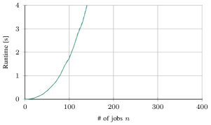
(a) 60s time granularity

(b) 15m time granularity

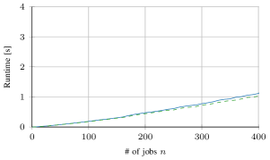
(c) 30m time granularity

(d) 1h time granularity

Figure 3: Runtimes relative to instance size, for various time granularities, solved for the whole day and using shortest_augmenting_path().

In the analysis above, we considered instances for a full day. In a next step, we present results of experiments that consider instances starting at noon.

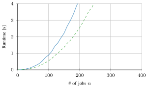
(a) 60s time granularity

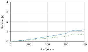
(b) 15m time granularity

(c) 30m time granularity

(d) 1h time granularity

Figure 4: Runtimes for instances solved at noon using shortest_augmenting_path().

Figure 4 shows the total runtimes of Focs and Focs-pm relative to instance size $n$ for the four time granularities, and maximum flow method shortest_augmenting_path(). However, as opposed to Figure 3, instances are solved starting from noon. As expected, for situations with the same instance size and time granularity, solving the (smaller) problem at noon is faster than solving the entire day. Furthermore, the added value of the pre-mature stop feature is even more pronounced in the noon experiments. For time granularities of 1 minute, 15 minutes, 30 minutes and 1 hour, the experiments show runtime improvements of at most 44%, 39%, 37% and 38% respectively for up to 400 EVs. That maximum improvement of the median runtime corresponds to instance sizes 400, 390, 290 and 340, all rather large instances. The average improvements amount to 33%, 28%, 26% and 23% respectively.

IV-B Maximum flow method comparison

The efficiency of an algorithm in the context of an Mpc among others depends on the implementation. As mentioned in Section II-B, Focs relies on solving multiple maximum flow problems. Hereby, in theory it does not matter which concrete algorithm is used. However, since according to Table I the available maximum flow algorithms are non-linear, this section investigates their impact on the scalability of Focs for large groups of EVs.

As mentioned in Section III-B, networkx provides a number of functions that compute maximum flows. In particular, our experiments use the shortest_augmenting_path(), edmonds_karp(), preflow_push() and dinitz() functions from the networkx package. Table I provides an overview of those functions, and the following three properties. First, per function, we cite the theoretical complexity of its namesake based on [12]. Note that the implementations of shortest_augmenting_path(), edmonds_karp(), preflow_push() and dinitz() likely do not strictly follow the original algorithms ([14], [15], [16]/[17] and [18] respectively). Since their publication, various improvements and variants have been introduced that are usually referred to by the same name. Secondly, Table I presents the theoretical complexity as reported by networkx. Finally, the last column takes the complexity reported by networkx and bounds the theoretical complexity specifically for flow networks of Focs instances. We note that the number of nodes (compare flow network in Figure 1) is bound by 2 plus the number of jobs and intervals, being $2+n+(2n-1)=3n+1$. The number of edges is roughly bound by $n+n(2n-1)+(2n-1)=2n^{2}+2n-1$. We derive the theoretical complexity in terms of the input size of Focs instances by substituting this in the bound reported by networkx. Since these maximum flow solvers are only used in the solving of Focs (and therefore do not influence the model building), we restrict the discussion of the results to the solving part of the runtime.

Figure 5 presents the solving time of Focs for a full day and quarterly time granularity. Among the methods using augmenting paths, we see a clear difference in performance between methods. While the time taken to solve Focs using shortest_augmenting_path() seems to grow almost linearly for instance sizes up to 400, solving times with edmonds_karp() and dinitz() clearly increase non-linearly. Finally, the preflow-push method behaves similarly to shortest_augmenting_path().

If we compare this to the theoretical complexity of the various maximum flow methods embedded in networkx (see Table I), the most striking observation is that while preflow_push() has the smallest theoretical runtime on Focs networks ($\mathcal{O}(n^{3})$), the theoretically quartic runtime of shortest_augmenting_path() ($\mathcal{O}(n^{4})$) outperforms the other tested methods. Edmonds_karp() shows the highest theoretical complexity, and empirically is the second slowest method, overtaken only by dinitz().

Overall, shortest_augmenting_path() appears to be the dominating method in our experiments with respect to runtime. The experiments further indicate that the proper choice of maximum flow method greatly increases the usability of Focs for EV scheduling.

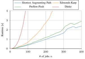
Figure 5: Runtimes for solving only for quarterly granularity, comparing maximum flow algorithms applied in Focs.

IV-C Runtime comparison

In the following, we compare Focs to the QP implementation for comparison with (commercial) optimization tools already available for Mpcs. The total runtime (i.e., the sum of the model building and solving), relative to instance size $n$ for the four time granularities is depicted in Figure 6. Note that for Focs, we assume that the flow method shortest_augmenting_path() is applied. All instances are solved for the full day.

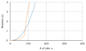
(a) 60s time granularity

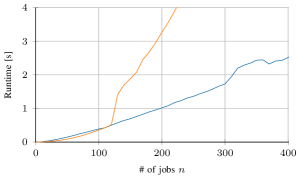
(b) 15m time granularity

(c) 30m time granularity

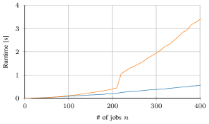
(d) 1h time granularity

Figure 6: Runtimes relative to instance size, for various time granularities, solved for the whole day and using shortest_augmenting_path().

First, we note that across subfigures, the quadratic program solved in Gurobi initially either outperforms Focs or runs at similar speed. However, we observe a gradually steeper increase in runtime relative to instance size for QP compared to the Focs model. As a result, the median runtime of Focs outperforms QP starting from instance sizes of approximately 90, 120, 90 and 80 for time granularities of 1 minute, 15 minutes, 30 minutes and 1 hour respectively. Furthermore, we observe a sudden steep increase in the runtime of the QP implementation, at instance sizes from around 90, 130, 170 and 230 in Figures 6a, 6b, 6c and 6d respectively. This behaviour possibly reflects that a certain memory threshold is reached after which solving becomes more costly for Gurobi due to swapping memory.

Overall, as expected, a finer time granularity for a given instance size results in a larger runtime for both the QP and Focs. Notably, the slope of the runtime for Focs seems to be almost linear for the instance sizes considered, except in Figure 6a. There, a non-linear increase can be observed. To give an indication of this growth, the median runtimes for Focs and QP with instance size 400 under time granularity 1 minute are respectively 36 and 62 seconds.

In a next step, we disaggregate the runtimes into model building and solving components (see Figure 7).

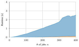
(a) Focs

(b) QP

Figure 7: Runtimes disaggregated into model building and solving for 15 m granularity.

Figure 7a presents the results for Focs, whereas Figure 7b presents the results for QP. Both figures are stackplots, depicting the total runtime as sum of the model building (bottom part, orange shading) and solving (top part, blue shading). The results correspond to experiments with time granularity of 15 minutes and shortest_augmenting_path() applied within Focs.

Notably, Focs spends most of its computation time on solving. The almost negligible contribution of model building can be attributed to the mostly dictionary-based implementation of flows in the networkx package. For QP, on the other hand, model building makes up a considerable portion of the runtime. Moreover, Figure 7b clearly attributes the earlier observed sudden steep increase in the runtime of the QP (discussed above) to its solving. This can be seen in the continued smooth increase in the bottom (orange) area, whereas approximately at instance size 130 the contribution of the solving time to the total runtime increases drastically.

V Discussion

In the previous section, we have presented the empirical results of our experiments. Next, we want to shortly discuss some of the limitations of this research, and put the results in perspective to physical parking lots for EV charging with Mpc.

First, we consider the implementation of Focs as used for the experiments. While the overall Focs method builds on augmentation of flows, within the used implementation the number of considered intervals is reduced between consecutive iterations and a new maximum flow with the empty flow as initialization is executed. A more efficient implementation would use the flow from the previous iteration, and augment on top of that. Especially if Focs uses a maximum flow method that relies on augmenting paths, this would speed up the optimization.

Moreover, in Mpc settings, both efficiency and quality of the optimization are crucial. Therefore, it is important to note that for the conclusions of Section IV-B we have not considered the exact form of the found schedule but focused solely on the runtime of the various flow methods. However, in the setting of EV scheduling, the fairness, robustness and user acceptability of the found schedule itself are of great importance. To illustrate, consider the example in Figure 8.

$j$	$a_{j}$	$d_{j}$	$e_{j}$	$p_{j}^{\max}$
1	0	2	2	2
2	0	1	$\frac{1}{2}$	2
3	1	2	$\frac{1}{2}$	2
4	0	2	2	2

Figure 8: Example of an instance where shortest_augmenting_path() results in a schedule with bias for one job over the other.

Here, jobs 1 and 4 share the same properties. The example provides two schedules. In the schedule on the left those two jobs are scheduled consecutively in disjoint intervals, whereas on the right they are scheduled in parallel. Both schedules are optimal solutions to the problem with constraints (1) minimizing objective function (3). One may argue, however, that the schedule on the right is fairer to the users and more robust to early departure of either job. Such considerations were left out of scope of this work, but should be considered in future work considering optimization in Mpc settings.

Finally, in the comparison of Focs to QP, we do not take the adaptivity of the models in an Mpc setting into account. While the model building for QP takes considerable time, Gurobi is known for efficiently altering and re-solving its models, using previous results in its initialization. This was left out of scope for the comparison. While we do recommend future work in that direction, we first suggest to conduct theoretical research on the efficient initialization of Focs and to implement the subsequent results to allow for a reasonable comparison.

VI Conclusion

This work investigated potential algorithms for an optimization subroutine in model predictive controllers for EV scheduling. To this end, we introduced a pre-mature stop feature for Focs, an algorithm suitable for this subroutine. The proposed feature can decrease runtime in Mpc settings. It is particularly effective close to peak hours, for example around noon at an office parking lot when parking lot occupancy is expected to be at its peak. Using a 15 minute granularity, the proposed variant of Focs shows a median runtime improvement of on average 28% compared to the original unadapted version to calculate a charging schedule at noon. Moreover, this work has illustrated the considerable impact of the chosen maximum flow method for Focs. Finally, for large EV parking lots, the presented runtimes show the competitiveness of Focs with commercial state-of-the-art optimization software.

Future work may dive deeper into the integration of Focs into an Mpc, and into the properties of the found schedules depending on the used maximum flow method.

References

- [1] R. Wolbertus and R. van den Hoed, Plug-in (Hybrid) Electric Vehicle Adoption in the Netherlands: Lessons Learned. Cham: Springer International Publishing, 2020, pp. 121–143.
- [2] N. Sadeghianpourhamami, N. Refa, M. Strobbe, and C. Develder, “Quantitive analysis of electric vehicle flexibility: A data-driven approach,” International Journal of Electrical Power & Energy Systems, vol. 95, pp. 451–462, 2018.
- [3] G. J. Osório, M. Gough, M. Lotfi, S. F. Santos, H. M. Espassandim, M. Shafie-khah, and J. P. Catalão, “Rooftop photovoltaic parking lots to support electric vehicles charging: A comprehensive survey,” International Journal of Electrical Power & Energy Systems, vol. 133, p. 107274, 2021.
- [4] J. W. Eising, T. van Onna, and F. Alkemade, “Towards smart grids: Identifying the risks that arise from the integration of energy and transport supply chains,” Applied Energy, vol. 123, pp. 448–455, 2014.
- [5] K. Turitsyn, N. Sinitsyn, S. Backhaus, and M. Chertkov, “Robust broadcast-communication control of electric vehicle charging,” in 2010 First IEEE International Conference on Smart Grid Communications, 2010, pp. 203–207.
- [6] M. Cañigueral and J. Meléndez, “Flexibility management of electric vehicles based on user profiles: The arnhem case study,” International Journal of Electrical Power & Energy Systems, vol. 133, p. 107195, 2021.
- [7] G. Vecchio and L. Tricarico, ““may the force move you”: Roles and actors of information sharing devices in urban mobility,” Cities, vol. 88, pp. 261–268, 2019.
- [8] Q. Zhou and C. Du, “A quantitative analysis of model predictive control as energy management strategy for hybrid electric vehicles: A review,” Energy Reports, vol. 7, pp. 6733–6755, 2021.
- [9] L. Winschermann, M. E. T. Gerards, A. Antoniadis, G. Hoogsteen, and J. Hurink, “Relating electric vehicle charging to speed scaling with job-specific speed limits,” 2023.
- [10] Gurobi Optimization, LLC, “Gurobi Optimizer Reference Manual,” 2023. [Online]. Available: https://www.gurobi.com
- [11] A. A. Hagberg, D. A. Schult, and P. J. Swart, “Exploring network structure, dynamics, and function using networkx,” in Proceedings of the 7th Python in Science Conference, G. Varoquaux, T. Vaught, and J. Millman, Eds., Pasadena, CA USA, 2008, pp. 11 – 15.
- [12] O. Cruz-Mejía and A. N. Letchford, “A survey on exact algorithms for the maximum flow and minimum-cost flow problems,” Networks, vol. 82, no. 2, pp. 167–176, 2023.
- [13] B. Nijenhuis, L. Winschermann, N. Bañol Arias, G. Hoogsteen, and J. L. Hurink, “Protecting the distribution grid while maximizing ev energy flexibility with transparency and active user engagement,” in CIRED Porto Workshop 2022: E-mobility and power distribution systems, vol. 2022, 2022, pp. 209–213.
- [14] L. R. Ford and D. R. Fulkerson, “Maximal flow through a network,” Canadian Journal of Mathematics, vol. 8, p. 399–404, 1956.
- [15] J. Edmonds and R. M. Karp, “Theoretical improvements in algorithmic efficiency for network flow problems,” J. ACM, vol. 19, no. 2, p. 248–264, apr 1972.
- [16] A. Karzanov, “Determining the maximal flow in a network by the method of preflows,” Doklady Mathematics, vol. 15, p. 434–437, 02 1974.
- [17] A. V. Goldberg and R. E. Tarjan, “A new approach to the maximum-flow problem,” J. ACM, vol. 35, no. 4, p. 921–940, oct 1988.
- [18] Y. Dinitz, “Algorithm for solution of a problem of maximum flow in networks with power estimation,” Soviet Math. Dokl., vol. 11, pp. 1277–1280, 01 1970.