singular profile of free boundary of incompressible inviscid fluid with external force

Abstract.

This article is devoted to investigate the singular profile of the free boundary of two-dimensional incompressible inviscid fluid with external force near the stagnation point. More precisely, given an external force with some polynomial type decay close to the stagnation point, the singular profile of the free boundary at stagnation point possible are corner wave, flat and cusp singularity. Through excluding the cusp and flat singularity, we know the only singular profile is corner wave singularity, and the corner depends on the decay rate of the solution near the stagnation point. The analysis depends on the geometric method to a class of Bernoulli-type free boundary problem with given degenerate gradient function on free boundary. This work is motivated by the significant work [E. V$\breve{a}$rv$\breve{a}$ruc$\breve{a}$ and G. Weiss, Acta Math, 206, 363-403, (2011)] on Stokes conjecture to the incompressible inviscid fluid acted on by gravity.

keyword: Free boundary; Singular profile; Euler flow; External force; Blow-up;
2020 Mathematics Subject classification: 76B15; 35Q31; 35R35

1. Background and main results

The mathematical problem of this paper concerns the motion of the interface separating an invisid, incompressible, irrotational fluid, under the influence of an external force f , from a region of air in 2-dimensional space. The interface between air and fluid is called the free boundary, see Fig. 1.

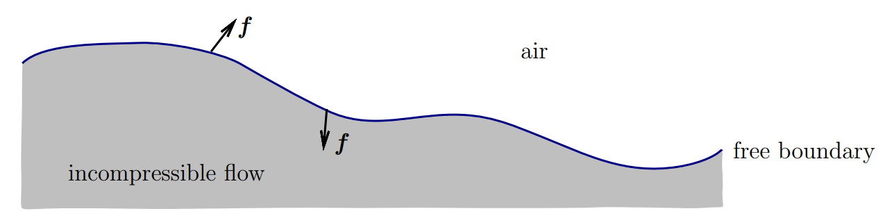
Figure 1. Physical model

The study of flows with free boundary between fluid and air has long fascinated both hydrodynamicists and mathematicians, and there is an extensive literature on the mathematical theory of ideal fluid under the action of external forces such as gravity, Coriolis force, electromagnetic force, etc.

The classical problem concerning the motion of water waves under the influence of gravity (e.g., water waves on the surface of the ocean) was first formulated by Isaac Newton in 1687, and then there have been some important recent advances, we refer to [19] and [28] for two dimensional water waves problem neglecting surface tension.

On the other hand, the effect of solid-body rotation of the earth produces Coriolis acceleration, which has led to the creation of Coriolis force named after Coriolis in 1835. Water waves under the influence of Coriolis force are very common in the physics literature, two dimensional obliquely rotating shallow water equations describing a thin inviscid fluid layer flowing over topography in a frame rotating about an arbitrary axis [14], an investigation of shallow water equations currents on the propagation of tsunamis [8] and two-dimensional Camassa-Holm equation arises in the modeling of the propagation of shallow water waves over a flat bed [18].

It is well-known that the external forces will significantly affect the dynamic motion of incompressible flows. Consequently, a central aim of this paper is to investigate the shape of the free boundary at stagnation points under the polynomial type decay of external forces.

1.1. Mathematical setting of physical problem

The steady planar flow of an ideal irrotational fluid, which is governed by the isentropic incompressible Euler equations with external forces

$$\begin{cases}\operatorname{div}\textbf{u}=0,\\ (\textbf{u}\cdot\nabla)\textbf{u}+\nabla p=\textbf{{f}},\end{cases}$$

where the unknown vector functions $\textbf{u}=(u_{1}(x,y),u_{2}(x,y))$ and scalar function $p(x,y)$ are the fluid velocity and pressure, respectively, and f describes the external force.

Assume the fluid is a zero-vorticity flow characterized by irrotational condition

$$\operatorname{curl}{\textbf{u}}=0.$$

And consequently, the external force f is assumed to be conservative, which means that there exists a function $F(x,y)$ such that

$$\textbf{{f}}=\nabla F.$$

Then, we can integrate the equation of momentum energy conservation to obtain Bernoulli’s law

$$\dfrac{1}{2}|\textbf{u}|^{2}+p-F(x,y)=\mathcal{B},$$

where $\mathcal{B}$ is the so-called Bernoulli’s constant.

On the free boundary, the fluid satisfies the following slip boundary condition

$\textbf{u}\cdot\textbf{{n}}=0$.

The equation of mass conservation implies that there exists stream function $u(x,y)$ such that

$u_{1}=\partial_{y}u$ and $u_{2}=-\partial_{x}u$.

Then, it is easy to check out that $u(x,y)$ is harmonic throughout the flow region in view of irrotational condition, whereas the slip boundary condition implies that the free boundary is a level set of $u(x,y)$. Without loss of generality, one assume that $\partial\{u>0\}$ and $\{u>0\}$ are the free boundary of the fluid and the fluid region, respectively. While ignoring surface tension, the constant pressure condition holds on the free boundary

$$p=p_{atm},$$

where $p_{atm}$ is the given constant atmopheric pressure.

The Bernoulli’s law gives the gradient condition on the free boundary

$|\nabla u|^{2}=h(x,y):=2\left(\mathcal{B}-p_{atm}+F(x,y)\right)\,\,\,\,$ on $\partial\{u>0\}$.

Since our aim is to get the local singularities, we focus on bounded domain $\Omega$ which has a non-empty intersection with the free boundary. Along with the harmonic equation, we formulate the following local Bernoulli-type free boundary problem

$$\begin{cases}\Delta u=0&\text{in}\,\Omega\cap\{u>0\},\\ \left|\nabla u\right|^{2}=h(x,y)\,\,&\text{on}\,\Omega\cap\partial\{u>0\}.\end{cases}$$ (1.1)

Remark 1.1.

It must be noted that the Bernoulli-type free boundary problem above can also describe a traveling wave moving at constant speed on the surface of an incompressible, inviscid, irrotational fluid.

1.2. Bernoulli-type free boundary problem

The Bernoulli-type free boundary problem is one of important unconstrained free boundary problems, which arises naturally in a number of physical phenomena. We would like to refer the famous survey [16] by A. Figalli and H. Shahgholian on it to the readers. The solution of Bernoulli-type free boundary problem solves the Laplace’s equation in the positive set and satisfies not only the homogeneous Dirichlet boundary condition, but also the Neumann boundary condition on the free boundary.

To investigate the properties of free boundary, the Bernoulli-type problem (1.1) usually can be divided into two cases according to whether the gradient function $h(x,y)$ degenerates near the free boundary point. The first case is that the gradient function $h(x,y)$ is non-degenerate, namely, there exists a positive constant $c_{0}$, such that $h(x,y)\geq c_{0}>0$ on the free boundary. The other case is that there exists a free boundary point $(x^{0},y^{0})$, such that $h(x^{0},y^{0})=0$. The point $(x^{0},y^{0})$ is called as the degenerate point of free boundary. In hydrodynamics, a point on the streamline where the velocity is zero is called a stagnation point.

The research on the regularity close to the non-degenerate free boundary point can be dated back to the pioneering work [2] by H. Alt and L. Caffarelli in 1981, in which they have showed that there is no singular point on the free boundary in two dimensions, that is to say, free boundary is locally in $\Omega$ a $C^{1,\alpha}$-surface. However, for higher dimensions ($n\geq 3$), G. Weiss in [26] first realized that there existed a maximal dimension $d^{*}$, such that the singular of the free boundary could occur only when $n\geq d^{*}$. Furthermore, it was asserted that $d^{*}\geq 4$ in [9], and $d^{*}\geq 5$ in [20]. Nevertheless, the regularity theory are widely applied to the physical model with free surface, such as incompressible inviscid jet in [3, 4, 5, 11], compressible impinging jet in [10] and incompressible impinging jet in [12] and so on.

On another hand, the singular wave profile will arise close to the degenerate point of the free boundary, even in two dimensions. This is also related to a very important topic in inviscid water wave, the so-called Stokes conjecture. In 1880, G. Stokes conjectured that the free surface of the two-dimensional inviscid irrotational water wave had a symmetric corner of 120 degree at any stagnation point. It has been shown firstly under some structural assumptions by C. Amick, L. Fraenkel and J. Toland [6] in 1982 and P. Plotnikov [21] in 2002 independently due to the so-called Nekrasov integral equation. An important breakthrough in the analysis of singular profile is due to the brilliant work [23] by E. V$\breve{a}$rv$\breve{a}$ruc$\breve{a}$ and G. Weiss. They introduced creatively a geometric method to give a rigorous and visual proof to the Stokes conjecture, and all the structural assumptions on the free boundary in the previous work were removed. The proof was based on the blow-up analysis, the monotonicity formula and the frequency formula. Furthermore, the geometric method has also been corroborated to be powerful to deal with the 2D rotational flow [24], and the axisymmetric flow in gravitational field [25, 13]. The mathematical problem in [23] to attack the Stokes conjecture is formulated into the following two-dimensional one-phase Bernoulli-type free boundary problem

$$\begin{cases}\Delta u=0&\text{in}\,\Omega\cap\{u>0\},\\ \left|\nabla u\right|=\sqrt{2\left(\mathcal{B}-p_{atm}-gy\right)}\,\,&\text{on}\,\Omega\cap\partial\{u>0\},\end{cases}$$

where $g$ is the gravity constant. The force of gravity acting vertically downward is the unique external force considered in [23]. The one key point in the analysis in [23] is that the gradient condition on the free boundary implies the behavior of solution near the stagnation point, that is, $u$ goes like $r^{3/2}$ near the stagnation point.

The main motivation of this paper is to consider the singularity of the free boundary to the Euler flow with general external force and meanwhile to analyze the one-phase Bernoulli-type free boundary problem (1.1) with general gradient function $h(x,y)$. To the end of this paper, we assume the gradient function

$$h(x,y)=C|x^{0}-x|^{\alpha}|y^{0}-y|^{\beta},\,\,\,\,\text{ for }\alpha\geq 0,\,\beta\geq 0,\alpha+\beta>0\,\text{and some constant}\,C,$$ (1.2)

the set of stagnation points is $\{X=(x,y)|X\in\Omega\cap\partial\{u>0\}\cap(\{x=x^{0}\}\cup\{y=y^{0}\})\}$. The problem (1.1) becomes as follows

$$\begin{cases}\Delta u=0\,\,&\text{in $\Omega\cap\{u>0\}$ },\\ \left|\nabla u\right|^{2}=C|x^{0}-x|^{\alpha}|y^{0}-y|^{\beta}\,\,&\text{on $\Omega\cap\partial\{u>0\}$}.\end{cases}$$

After some normalization, the above problem can then be described by

$$\begin{cases}\Delta u=0\,\,&\text{in $\Omega\cap\{u>0\}$ },\\ \left|\nabla u\right|^{2}=h_{0}(x,y):=|x|^{\alpha}|y|^{\beta}\,\,&\text{on $\Omega\cap\partial\{u>0\}$}.\end{cases}$$ (1.3)

In this paper, we focus on the weak solution to the local Bernoulli-type free boundary problem (1.3) in $\Omega$ in the distributional sense, and we omit the boundary condition on $\partial\Omega$.

Obviously, the energy function formally associated with the problem (1.3) is

$$J(u):=\int_{\Omega}\left(\left|\nabla u\right|^{2}+|x|^{\alpha}|y|^{\beta}\chi_{\{u>0\}}\right)dX,$$

which helps us define the weak solution later.

Remark 1.2.

It must be remarked that gradient condition on the free boundary implies that the external force in form is

$$\textbf{{f}}=\nabla F=\dfrac{1}{2}\nabla h_{0}(x,y)=\frac{1}{2}\left(\alpha|x|^{\alpha-1}|y|^{\beta}\operatorname{sgn}(x),\beta|x|^{\alpha}|y|^{\beta-1}\operatorname{sgn}(y)\right),$$

when $x\neq 0$ and $y\neq 0$, here the function $\operatorname{sgn}(t)$ denotes the sign function of $t$.

In what follows, we denote $X_{0}=(x_{0},y_{0})\in\Omega\cap\partial\{u>0\}$ be the possible stagnation point of the free boundary, and analyze the singular wave profile of the Bernoulli-type free boundary problem (1.3). All the possible stagnation points will fall into one of three following categories (see Fig. 2).

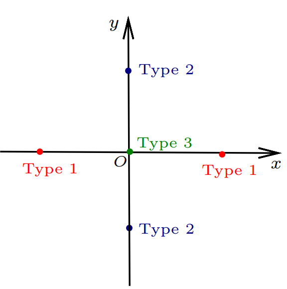
Figure 2. Three types stagnation points

Case 1. (Type 1 stagnation point) $X_{0}=(x_{0},0)$, for $x_{0}\neq 0$. Since the $x$ direction is non-degenerate, the singularity arises only in the $y$ direction, and we suppose that $\beta\geq 1$;

Case 2. (Type 2 stagnation point) $X_{0}=(0,y_{0})$, for $y_{0}\neq 0$. Since the $y$ direction is non-degenerate, the singularity arises only in the $x$ direction, and we suppose that $\alpha\geq 1$;

Case 3. (Type 3 stagnation point) $X_{0}=(0,0)$. The singularity arises both in the $x$ and $y$ direction, and we suppose that $\alpha\geq 1$ and $\beta\geq 1$.

In addition, $h(x,y)$ can imply the direction of the external force f in Case 1 and 2, briefly speaking, the direction of the force is vertical for Case 1, and the direction of the force is horizontal for Case 2.

According to the direction of the force and the location of the stagnation point, we take Case 1 as an example to explain in detail how to classify,

$$\lim\limits_{x\rightarrow x_{0},y\rightarrow 0\pm}\dfrac{\partial_{y}h_{0}(x,y)}{\partial_{x}h_{0}(x,y)}=\lim\limits_{x\rightarrow x_{0},y\rightarrow 0\pm}\arctan\dfrac{\beta x}{\alpha y}=\pi\mp\frac{\pi}{2},\,\,\,\text{for }\,\,\,x_{0}<0,$$

and

$$\lim\limits_{x\rightarrow x_{0},y\rightarrow 0\pm}\dfrac{\partial_{y}h_{0}(x,y)}{\partial_{x}h_{0}(x,y)}=\lim\limits_{x\rightarrow x_{0},y\rightarrow 0\pm}\arctan\dfrac{\beta x}{\alpha y}=\pi\mp\frac{\pi}{2},\,\,\,\text{for }\,\,\,x_{0}>0.$$

Then we denoting the limit above is $\theta_{0}$, which is the deflection angle down from the positive $x$-axis of f at the point $(x_{0},0)$. Based on the above observation and the direction of the force near the stagnation point, we can divide Case 1 into (see Fig. 3)

Subcase 1.1. (Type 1 stagnation point) $x_{0}<0$ and $\theta_{0}=\frac{3\pi}{2}$;

Subcase 1.2. (Type 1 stagnation point) $x_{0}>0$ and $\theta_{0}=\frac{\pi}{2}$;

Subcase 1.3. (Type 1 stagnation point) $x_{0}<0$ and $\theta_{0}=\frac{\pi}{2}$;

Subcase 1.4. (Type 1 stagnation point) $x_{0}>0$ and $\theta_{0}=\frac{3\pi}{2}$.

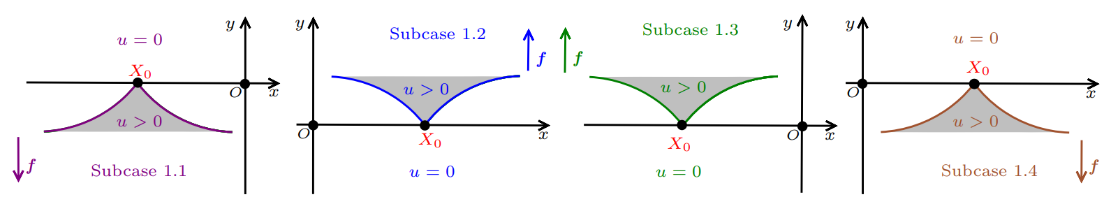
Figure 3. Type 1 stagnation points

Remark 1.3.

For the special case (Subcase 1.1 and Subscase 1.4), $\alpha=0$ and $\beta=1$, the free boundary problem (1.3) is nothing but the water wave problem under gravity which was discussed in [23] by E. V$\breve{a}$rv$\breve{a}$ruc$\breve{a}$ and G. Weiss.

It is easy to see that the direction of the force is $0$ or $\pi$ in Case 2, and the stagnation point is $(0,y_{0})$. It follows that Case 2 is divided into the following subcases (see Fig. 4)

Subcase 2.1. (Type 2 stagnation point) $y_{0}<0$ and $\theta_{0}=\pi$;

Subcase 2.2. (Type 2 stagnation point) $y_{0}>0$ and $\theta_{0}=0$;

Subcase 2.3. (Type 2 stagnation point) $y_{0}<0$ and $\theta_{0}=0$;

Subcase 2.4. (Type 2 stagnation point) $y_{0}>0$ and $\theta_{0}=\pi$.

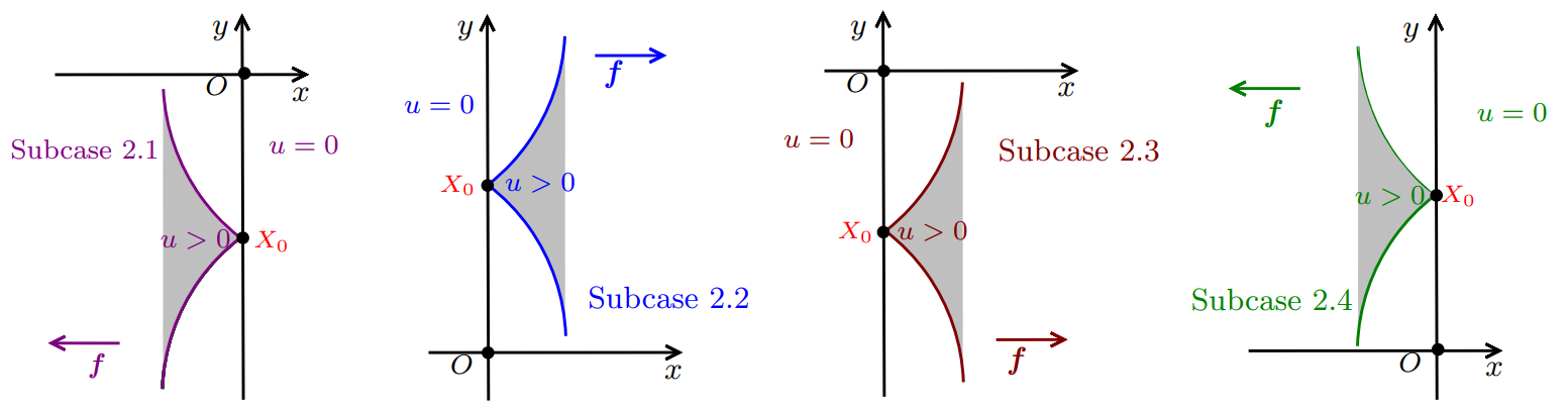
Figure 4. Type 2 stagnation points

Roughly speaking, the gradient assumption in (1.3) gives the deflection angle of the external force at Type 1 and Type 2 stagnation points. However, for Case 3, the gradient condition $\left|\nabla u\right|^{2}=|x|^{\alpha}|y|^{\beta}$ implies that the external force $\textbf{{f}}=\nabla h_{0}(x,y)$ vanishes at the origin, and the deflection angle of the external force is not well defined.

In this paper, we mainly focus on the asymptotic singular profile of the wave near the stagnation point, and denote $\theta^{*}$ the angle bisector of the asymptotic directions of the free boundary. Moreover, we conjecture that a reasonable conclusion is that the direction of the force coincides the angle $\theta^{*}$, that is to say $\theta_{0}=\theta^{*}$. This conjecture will be confirmed in Case 1 and Case 2. However, since the force vanishes at the stagnation point in Case 3, so the direction of the force is missing now. Therefore, we have to give an additional assumption on the angle bisector $\theta^{*}$ of the asymptotic directions of free boundary for Case 3.

Case 3. Type 3 stagnation point. $X_{0}=(0,0)$, we denote $\nu^{*}=(\cos\theta^{*},\sin\theta^{*})$. See Fig. 5.

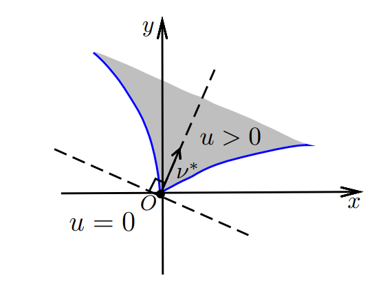
Figure 5. Type 3 stagnation point

1.3. Definitions and assumptions

In this subsection, we give the definitions of weak solution, blow-up sequence, blow-up limit and weighted density.

Definition 1.4.

(Stagnation points). We call

$$S^{u}:=\left\{X=(x,y)|X\in\Omega\cap\partial\{u>0\}\cap(\{x=0\}\cup\{y=0\})\right\}$$

as the set of stagnation points.

Definition 1.5.

(Weak solution) A non-negative function $u\in W_{\operatorname{loc}}^{1,2}(\Omega)$ is defined a weak solution of (1.3) in $\Omega$, if

(i) $u\in C^{0}(\Omega)\cap C^{2}\left(\Omega\cap\{u>0\}\right)$, $u\geq 0$ in $\Omega$, $u\equiv 0$ in $\{X|(X-X_{0})\cdot(\cos\theta_{0},\sin\theta_{0})<0\}$;

(ii) the first variation with respect to domain variations of the functional

$$J(v):=\int_{\Omega}\left(\left|\nabla v\right|^{2}+|x|^{\alpha}|y|^{\beta}\chi_{\{v>0\}}\right)dX$$

vanishes at $v=u$, and $\chi_{\{v>0\}}$ is the characteristic function of a set ${\{v>0\}}$. Equivalently,

$$0= -\frac{d}{d\varepsilon}J\left(u\left(X+\varepsilon\phi(X)\right)\right)\Big{|}_{\varepsilon=0}$$ (1.4)

$$= \int_{\Omega}\Big{[}\left|\nabla u\right|^{2}\operatorname{div}\phi-2\nabla uD\phi\nabla u+|x|^{\alpha}|y|^{\beta}\operatorname{div}\phi\chi_{\{u>0\}}$$

$$+\big{(}\alpha|x|^{\alpha-1}|y|^{\beta}\phi_{1}\operatorname{sgn}(x)+\beta|x|^{\alpha}|y|^{\beta-1}\phi_{2}\operatorname{sgn}(y)\big{)}\chi_{\{u>0\}}\Big{]}dX$$

for any $\phi=(\phi_{1},\phi_{2})\in C_{0}^{1}(\Omega;\mathbb{R}^{2}),$ we denote $dX=dxdy$ throughout this paper;

(iii) the topological free boundary $(\partial\{u>0\}\cap\Omega)\backslash S^{u}$ is locally a $C^{2,\gamma}$-surface for some $\gamma\in(0,1)$.

Remark 1.6.

For Case 3, the force degenerates at the origin, which means that the force has no direction at this point. Hence we use $\theta^{*}$ instead of $\theta_{0}$ in the definition of the weak solution.

Remark 1.7.

Indeed, for the regularity of the topological free boundary, the fact (iii) in Definition 1.5 has been verified in the pioneer work [2] by H. Alt and L. Caffarelli.

We assume that the following Bernstein estimate holds close to the free boundary.

Assumption A.

In regards to the free boundary problem (1.3), let $u$ satisfy

$$|\nabla u|^{2}\leq C|x|^{\alpha}|y|^{\beta}$$ (1.5)

in $B_{r_{0}}(X_{0})$, for $X_{0}\in S^{u}$, and some $r_{0}>0$, $C$ is a positive constant.

Next, we will provide the definitions of the blow-up sequence for three types of stagnation points respectively. It is noticeable that the gradient condition $|\nabla u|^{2}=|x|^{\alpha}|y|^{\beta}$ on the free boundary implies the behavior of the weak solution $u$ close to the stagnation point. In other words, $u$ goes like $r^{\frac{\beta+2}{2}}$ near Type 1 stagnation point $X_{0}=(x_{0},0)$; $u$ goes like $r^{\frac{\alpha+2}{2}}$ near Type 2 stagnation point $X_{0}=(0,y_{0})$; $u$ goes like $r^{\frac{\alpha+\beta+2}{2}}$ near Type 3 stagnation point $X_{0}=(0,0)$. For this reason, we need to give the following definitions of rescaled functions.

Definition 1.8.

For every $r>0$, we define the rescaled functions

$u(X)=r^{\kappa_{i}}u(X_{0}+rX),\,\,\text{for}\,i=1,2,3,$

where $\kappa_{1}=-\frac{\beta+2}{2}$, $\kappa_{2}=-\frac{\alpha+2}{2}$ and $\kappa_{3}=-\frac{\alpha+\beta+2}{2}$ respectively for Type 1, 2 and 3 stagnation point. Let $\{r_{m}\}$ be a vanishing sequence of positive numbers as $m\rightarrow\infty$, we say that the sequence of function $u_{m}(X)=r_{m}^{\kappa}u(X_{0}+r_{m}X)$ is a blow-up sequence.

In addition, for each $r>0$, if the sequence $\{u_{m}(X)\}$ is uniformly bounded in $W^{1,2}(B_{r})$, there exists a subsequence converging to $u_{0}(X)$ weakly in $W^{1,2}(B_{r})$ as $m\rightarrow\infty$. Such the function $u_{0}(X)$ is called the blow-up limit of $u(X)$ at the stagnation point $X_{0}$, which indicate the infinitesimal behavior of $u(X)$ near $X_{0}$.

The following definitions are dedicated to the monotonicity formula for the adjusted boundary functional introduced by G. Weiss in [27]. Precisely, for three types of stagnation points, $u$ goes like $r^{\frac{\beta+2}{2}}$, $r^{\frac{\alpha+2}{2}}$ and $r^{\frac{\alpha+\beta+2}{2}}$ respectively, accordingly we define the Weiss adjusted boundary energies $M_{i}(r)$ as follows

$$M_{i}(r)=r^{2\kappa_{i}}\int_{B_{r}(X_{0})}\left(\left|\nabla u\right|^{2}+|x|^{\alpha}|y|^{\beta}\chi_{\{u>0\}}\right)dX+\kappa_{i}r^{2\kappa_{i}-1}\int_{\partial B_{r}(X_{0})}u^{2}d\mathcal{H}^{1},\,\text{for}\,i=1,2,3.$$ (1.6)

Remark 1.9.

In the next section, we will prove that the limits $M_{i}(r_{m})$ exist as $m\rightarrow\infty$ and denote the limits as $M_{i}(0+)$. Taking Subscase 1.1 , 2.1 and Case 3 as examples,

$$M_{1}(0+)=(-x_{0})^{\alpha}\lim\limits_{m\rightarrow\infty}\int_{B_{1}}(y_{-})^{\beta}\chi_{\{u_{m}>0\}}dX=(-x_{0})^{\alpha}\lim\limits_{m\rightarrow\infty}\dfrac{w_{2}\int_{B_{1}}(y_{-})^{\beta}\chi_{\{u_{m}>0\}}dX}{|B_{1}|};$$

$$M_{2}(0+)=(-y_{0})^{\beta}\lim\limits_{m\rightarrow\infty}\int_{B_{1}}(x_{-})^{\alpha}\chi_{\{u_{m}>0\}}dX=(-y_{0})^{\beta}\lim\limits_{m\rightarrow\infty}\dfrac{w_{2}\int_{B_{1}}(x_{-})^{\alpha}\chi_{\{u_{m}>0\}}dX}{|B_{1}|};$$

and

$$M_{3}(0+)=\lim\limits_{m\rightarrow\infty}\int_{B_{1}}|x|^{\alpha}|y|^{\beta}\chi_{\{u_{m}>0\}}dX=\lim\limits_{m\rightarrow\infty}\dfrac{w_{2}\int_{B_{1}}|x|^{\alpha}|y|^{\beta}\chi_{\{u_{m}>0\}}dX}{|B_{1}|},$$

where $y_{+}=\operatorname{max}\{y,0\}$ and $y_{-}=-\operatorname{min}\{y,0\}$, $w_{2}$ is the volume of the unit ball in two dimensions, which are equivalent to the weighted density of the set $\{u>0\}$ at $X_{0}$ in Subscase 1.1 , 2.1 and Case 3 respectively.

The notion of weighted density was first introduced by E. V$\breve{a}$rv$\breve{a}$ruc$\breve{a}$ and G. Weiss in [23], which can help us to understand the geometric structure of $\partial\{u>0\}$, which is a brilliant study, so we follow their definition here.

Under the previous assumptions, we are only able to achieve exact forms of the blow-up limit and weighted densities. In order to obtain the asymptotic behavior of free boundary, the following assumption is required.

Assumption B.

For $X_{0}\in S^{u}$, let $\partial\{u>0\}$ is a continuous injective curve $\sigma=(\sigma_{1}(t),\sigma_{2}(t)):I\rightarrow\mathbb{R}^{2}$ in a neighborhood of $X_{0}$, such that $\sigma(0)=X_{0}$, and $\sigma_{1}(t)-\sigma_{1}(0)\neq 0$ for $(-s,s)\backslash\{0\}$, where $I$ is an interval of $\mathbb{R}^{2}$ containing the origin and $s$ is a positive constant.

1.4. Main results

In this paper, we consider the asymptotic singularity profile of the free boundary to the Bernoulli-type free boundary problem (1.3), with boundary gradient function

$$h_{0}(x,y)=|x|^{\alpha}|y|^{\beta},$$

and give different singular profiles as follows, see Table 1 in Appendix.

Theorem 1.1.

(Type 1 stagnation point). Let $u$ be a weak solution of the free boundary problem (1.3) satisfying Assumption A and B. Then for $\alpha\geq 0$ and $\beta\geq 1$, at Type 1 stagnation point, the singular profile must be a $\frac{2\pi}{\beta+2}$-degree corner wave profile, that means the wave has a symmetric corner of $\frac{2\pi}{\beta+2}$ at the stagnation point. Moreover,

(1) for Subcase 1.1, the blow-up limit is

$u_{0}(X)=u_{0}(r\cos\theta,r\sin\theta)=\frac{2(-x_{0})^{\frac{\alpha}{2}}}{\beta+2}r^{\frac{\beta+2}{2}}\cos^{\frac{\beta}{2}}\left(\frac{\pi}{\beta+2}\right)\cos\left(\frac{\beta+2}{2}\theta+\frac{\beta+2}{4}\pi\right)\chi_{\left\{-\frac{\beta+4}{2(\beta+2)}\pi<\theta<-\frac{\beta}{2(\beta+2)}\pi\right\}},$

and the corresponding weighted density is

$$M_{1}(0+)=(-x_{0})^{\alpha}\int_{B_{1}\bigcap\left\{-\frac{\beta+4}{2(\beta+2)}\pi<\theta<-\frac{\beta}{2(\beta+2)}\pi\right\}}(y_{-})^{\beta}dX,$$

and

$$\lim\limits_{t\rightarrow 0\pm}\frac{\sigma_{2}(t)}{\sigma_{1}(t)-x_{0}}=-\tan\frac{\left(\beta+2\pm 2\right)\pi}{2(\beta+2)}\,\,\,\text{or}\lim\limits_{t\rightarrow 0\pm}\frac{\sigma_{2}(t)}{\sigma_{1}(t)-x_{0}}=-\tan\frac{\left(\beta+2\mp 2\right)\pi}{2(\beta+2)}.$$ (1.7)

The corner wave profile can be seen in Fig. 6(a).

(2) For Subcase 1.2, the blow-up limit is

$u_{0}(X)=u_{0}(r\cos\theta,r\sin\theta)=\frac{2x_{0}^{\frac{\alpha}{2}}}{\beta+2}r^{\frac{\beta+2}{2}}\sin^{\frac{\beta}{2}}\left(\frac{\beta}{2(\beta+2)}\pi\right)\cos\left(\frac{\beta+2}{2}\theta-\frac{\beta+2}{4}\pi\right)\chi_{\left\{\frac{\beta}{2(\beta+2)}\pi<\theta<\frac{\beta+4}{2(\beta+2)}\pi\right\}},$

and the corresponding weighted density is

$$M_{1}(0+)=x_{0}^{\alpha}\int_{B_{1}\bigcap\left\{\frac{\beta}{2(\beta+2)}\pi<\theta<\frac{\beta+4}{2(\beta+2)}\pi\right\}}(y_{+})^{\beta}dX,$$

and

$$\lim\limits_{t\rightarrow 0\pm}\frac{\sigma_{2}(t)}{\sigma_{1}(t)-x_{0}}=\tan\frac{\left(\beta+2\mp 2\right)\pi}{2(\beta+2)}\,\,\,\text{or}\lim\limits_{t\rightarrow 0\pm}\frac{\sigma_{2}(t)}{\sigma_{1}(t)-x_{0}}=\tan\frac{\left(\beta+2\pm 2\right)\pi}{2(\beta+2)}.$$

The corner wave profile can be seen in Fig. 6(b).

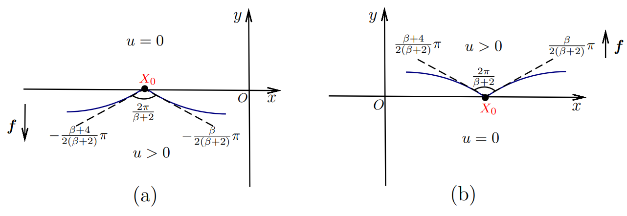
Figure 6. Singular profile for Subscase 1.1 and Subcase 1.2

(3) For Subcase 1.3, the blow-up limit is

$u_{0}(X)=u_{0}(r\cos\theta,r\sin\theta)=\frac{2(-x_{0})^{\frac{\alpha}{2}}}{\beta+2}r^{\frac{\beta+2}{2}}\sin^{\frac{\beta}{2}}\left(\frac{\beta}{2(\beta+2)}\pi\right)\cos\left(\frac{\beta+2}{2}\theta-\frac{\beta+2}{4}\pi\right)\chi_{\left\{\frac{\beta}{2(\beta+2)}\pi<\theta<\frac{\beta+4}{2(\beta+2)}\pi\right\}},$

and the corresponding weighted density is

$$M_{1}(0+)=(-x_{0})^{\alpha}\int_{B_{1}\bigcap\left\{\frac{\beta}{2(\beta+2)}\pi<\theta<\frac{\beta+4}{2(\beta+2)}\pi\right\}}(y_{+})^{\beta}dX,$$

and

$$\lim\limits_{t\rightarrow 0\pm}\frac{\sigma_{2}(t)}{\sigma_{1}(t)-x_{0}}=\tan\frac{\left(\beta+2\mp 2\right)\pi}{2(\beta+2)}\,\,\,\text{or}\lim\limits_{t\rightarrow 0\pm}\frac{\sigma_{2}(t)}{\sigma_{1}(t)-x_{0}}=\tan\frac{\left(\beta+2\pm 2\right)\pi}{2(\beta+2)}.$$

The corner wave profile can be seen in Fig. 7(a).

(4) For Subcase 1.4, the blow-up limit is

$u_{0}(X)=u_{0}(r\cos\theta,r\sin\theta)=\frac{2x_{0}^{\frac{\alpha}{2}}}{\beta+2}r^{\frac{\beta+2}{2}}\cos^{\frac{\beta}{2}}\left(\frac{\pi}{\beta+2}\right)\cos\left(\frac{\beta+2}{2}\theta+\frac{\beta+2}{4}\pi\right)\chi_{\left\{-\frac{\beta+4}{2(\beta+2)}\pi<\theta<-\frac{\beta}{2(\beta+2)}\pi\right\}},$

and the corresponding weighted density is

$$M_{1}(0+)=x_{0}^{\alpha}\int_{B_{1}\bigcap\left\{-\frac{\beta+4}{2(\beta+2)}\pi<\theta<-\frac{\beta}{2(\beta+2)}\pi\right\}}(y_{-})^{\beta}dX,$$

and

$$\lim\limits_{t\rightarrow 0\pm}\frac{\sigma_{2}(t)}{\sigma_{1}(t)-x_{0}}=-\tan\frac{\left(\beta+2\pm 2\right)\pi}{2(\beta+2)}\,\,\,\text{or}\lim\limits_{t\rightarrow 0\pm}\frac{\sigma_{2}(t)}{\sigma_{1}(t)-x_{0}}=-\tan\frac{\left(\beta+2\mp 2\right)\pi}{2(\beta+2)}.$$

The corner wave profile can be seen in Fig. 7(b).

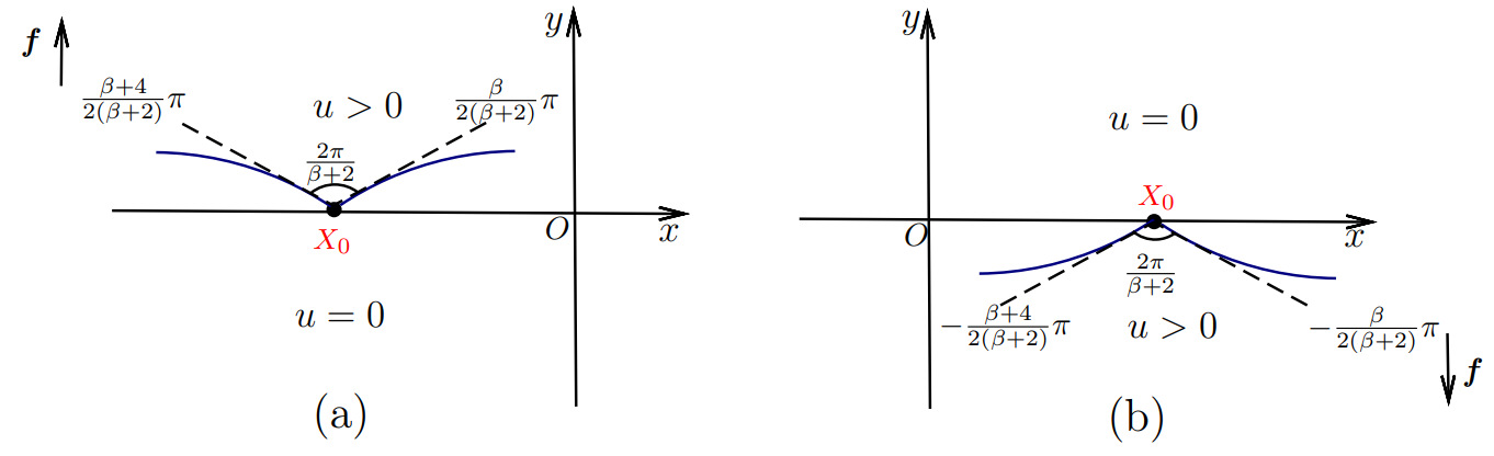
Figure 7. Singular profile for Subscase 1.3 and Subcase 1.4

Remark 1.10.

As mentioned in Theorem 1.1, the value of $\beta$ is closely related to the angle of the asymptotic directions of the free boundary. The angle of the asymptotic directions of the free boundary is $\frac{2\pi}{\beta+2}\in(0,\frac{2\pi}{3}]$. The larger $\beta$ is, the faster the solution decays, thus the angle becomes smaller.

Remark 1.11.

The reason there are two limits for the slope in (1.7) is that we do not require $t>0$ to indicate $X$ converging to $X_{0}$ from the positive direction, and at the same time we do not require $t<0$ to indicate $X$ converging to $X_{0}$ from the negative direction. But the geometrical meaning of them is the same and both represent two asymptotic directions of the free boundary that are unique.

Theorem 1.2.

(Type 2 stagnation point). Let $u$ be a weak solution of the free boundary problem (1.3) satisfying Assumption A and B. Then when $\alpha\geq 1$ and $\beta\geq 0$, at Type 2 stagnation point, the singular profile must be a $\frac{2\pi}{\alpha+2}$-degree corner wave profile, that means the wave has a symmetric corner of $\frac{2\pi}{\alpha+2}$ at the stagnation point. Moreover,

(1) for Subcase 2.1, the blow-up limit is

$u_{0}(X)=u_{0}(r\cos\theta,r\sin\theta)=\frac{2(-y_{0})^{\frac{\beta}{2}}}{\alpha+2}r^{\frac{\alpha+2}{2}}\cos^{\frac{\alpha}{2}}\left(\frac{\alpha+1}{\alpha+2}\pi\right)\cos\left(\frac{\alpha+2}{2}\theta+\frac{2-\alpha}{2}\pi\right)\chi_{\left\{\frac{\alpha+1}{\alpha+2}\pi<\theta<\frac{\alpha+3}{\alpha+2}\pi\right\}},$

and the corresponding weighted density is

$$M_{2}(0+)=(-y_{0})^{\beta}\int_{B_{1}\bigcap\left\{\frac{\alpha+1}{\alpha+2}\pi<\theta<\frac{\alpha+3}{\alpha+2}\pi\right\}}(x_{-})^{\alpha}dX,$$

and

$$\lim\limits_{t\rightarrow 0\pm}\frac{\sigma_{2}(t)-y_{0}}{\sigma_{1}(t)}=\tan\frac{\left(\alpha+2\pm 1\right)\pi}{\alpha+2}\,\,\text{or}\lim\limits_{t\rightarrow 0\pm}\frac{\sigma_{2}(t)-y_{0}}{\sigma_{1}(t)}=\tan\frac{\left(\alpha+2\mp 1\right)\pi}{\alpha+2}.$$

The corner wave profile can be seen in Fig. 8(a).

(2) For Subcase 2.2, the blow-up limit is

$u_{0}(X)=u_{0}(r\cos\theta,r\sin\theta)=\frac{2y_{0}^{\frac{\beta}{2}}}{\alpha+2}r^{\frac{\alpha+2}{2}}\cos^{\frac{\alpha}{2}}\left(\frac{\pi}{\alpha+2}\right)\cos\left(\frac{\alpha+2}{2}\theta\right)\chi_{\left\{-\frac{\pi}{\alpha+2}<\theta<\frac{\pi}{\alpha+2}\right\}},$

and the corresponding weighted density is

$$M_{2}(0+)=y_{0}^{\beta}\int_{B_{1}\bigcap\left\{-\frac{\pi}{\alpha+2}<\theta<\frac{\pi}{\alpha+2}\right\}}(x_{+})^{\alpha}dX.,$$

and

$$\lim\limits_{t\rightarrow 0\pm}\frac{\sigma_{2}(t)-y_{0}}{\sigma_{1}(t)}=\pm\tan\frac{\pi}{\alpha+2}\,\,\text{or}\lim\limits_{t\rightarrow 0\pm}\frac{\sigma_{2}(t)-y_{0}}{\sigma_{1}(t)}=\mp\tan\frac{\pi}{\alpha+2}.$$

The corner wave profile can be seen in Fig. 8(b).

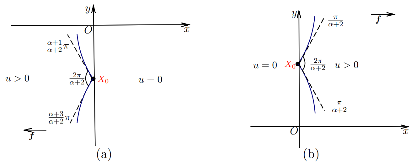
Figure 8. Singular profile for Subscase 2.1 and Subcase 2.2

(3) For Subscase 2.3, the blow-up limit is

$u_{0}(X)=u_{0}(r\cos\theta,r\sin\theta)=\frac{2(-y_{0})^{\frac{\beta}{2}}}{\alpha+2}r^{\frac{\alpha+2}{2}}\cos^{\frac{\alpha}{2}}\left(\frac{\pi}{\alpha+2}\right)\cos\left(\frac{\alpha+2}{2}\theta\right)\chi_{\left\{-\frac{\pi}{\alpha+2}<\theta<\frac{\pi}{\alpha+2}\right\}},$

and the corresponding weighted density is

$$M_{2}(0+)=(-y_{0})^{\beta}\int_{B_{1}\bigcap\left\{-\frac{\pi}{\alpha+2}<\theta<\frac{\pi}{\alpha+2}\right\}}(x_{+})^{\alpha}dX,$$

and

$$\lim\limits_{t\rightarrow 0\pm}\frac{\sigma_{2}(t)-y_{0}}{\sigma_{1}(t)}=\pm\tan\frac{\pi}{\alpha+2}\,\,\text{or}\lim\limits_{t\rightarrow 0\pm}\frac{\sigma_{2}(t)-y_{0}}{\sigma_{1}(t)}=\mp\tan\frac{\pi}{\alpha+2}.$$

The corner wave profile can be seen in Fig. 9(a).

(4) For Subscase 2.4, the blow-up limit is

$u_{0}(X)=u_{0}(r\cos\theta,r\sin\theta)=\frac{2y_{0}^{\frac{\beta}{2}}}{\alpha+2}r^{\frac{\alpha+2}{2}}\cos^{\frac{\alpha}{2}}\left(\frac{\alpha+1}{\alpha+2}\pi\right)\cos\left(\frac{\alpha+2}{2}\theta+\frac{2-\alpha}{2}\pi\right)\chi_{\left\{\frac{\alpha+1}{\alpha+2}\pi<\theta<\frac{\alpha+3}{\alpha+2}\pi\right\}},$

and the corresponding weighted density is

$$M_{2}(0+)=y_{0}^{\beta}\int_{B_{1}\bigcap\left\{\frac{\alpha+1}{\alpha+2}\pi<\theta<\frac{\alpha+3}{\alpha+2}\pi\right\}}(x_{-})^{\alpha}dX,$$

and

$$\lim\limits_{t\rightarrow 0\pm}\frac{\sigma_{2}(t)-y_{0}}{\sigma_{1}(t)}=\tan\frac{\left(\alpha+2\pm 1\right)\pi}{\alpha+2}\,\,\text{or}\lim\limits_{t\rightarrow 0\pm}\frac{\sigma_{2}(t)-y_{0}}{\sigma_{1}(t)}=\tan\frac{\left(\alpha+2\mp 1\right)\pi}{\alpha+2}.$$

The corner wave profile can be seen in Fig. 9(b).

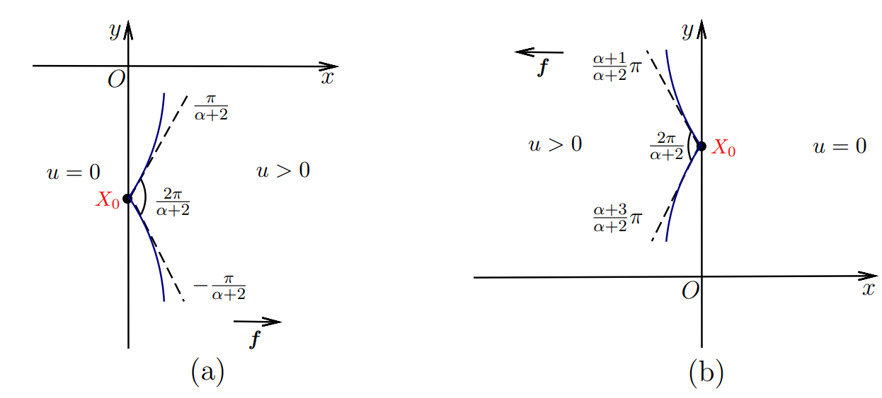
Figure 9. Singular profile for Subscase 2.3 and 2.4

Theorem 1.3.

(Type 3 stagnation point). Let $u$ be a weak solution of the free boundary problem (1.3) satisfying Assumption A and B, then for $\alpha\geq 1$ and $\beta\geq 1$, at Type 3 stagnation point, the singular profile must be a $\frac{2\pi}{\alpha+\beta+2}$-degree corner wave profile, that means the wave has a corner of $\frac{2\pi}{\alpha+\beta+2}$ at the stagnation point.

More precisely, at each Type 3 stagnation point, there exist $\theta_{1}$ and $\theta_{2}$, such that $\theta_{2}-\theta_{1}=\frac{2\pi}{\alpha+\beta+2}$ and satisfy the boundary condition of blow-up limit. The blow-up limit is as follows

$$u_{0}(X)= u_{0}(r\cos\theta,\sin\theta)$$

$$= \dfrac{2|\cos\theta_{1}|^{\frac{\alpha}{2}}|\sin\theta_{1}|^{\frac{\beta}{2}}}{\alpha+\beta+2}r^{\frac{\alpha+\beta+2}{2}}\cos\left(\frac{\alpha+\beta+2}{2}\theta+\arcsin\left|\cos\left(\frac{\alpha+\beta+2}{2}\theta_{1}\right)\right|\right)\chi_{\left\{\theta_{1}<\theta<\theta_{2}\right\}}.$$

And the corresponding density is

$$M_{3}(0+)=\int_{B_{1}\cap\left\{\theta_{1}<\theta<\theta_{2}\right\}}|x|^{\alpha}|y|^{\beta}dX,$$

and

$$\lim\limits_{t\rightarrow 0\pm}\frac{\sigma_{2}(t)}{\sigma_{1}(t)}=\tan\left(\dfrac{\theta_{1}+\theta_{2}}{2}\pm\dfrac{\theta_{1}-\theta_{2}}{2}\right)\,\,\text{or}\lim\limits_{t\rightarrow 0\pm}\frac{\sigma_{2}(t)}{\sigma_{1}(t)}=\tan\left(\dfrac{\theta_{1}+\theta_{2}}{2}\pm\dfrac{\theta_{2}-\theta_{1}}{2}\right).$$

The corner wave profile can be seen in Fig. 10.

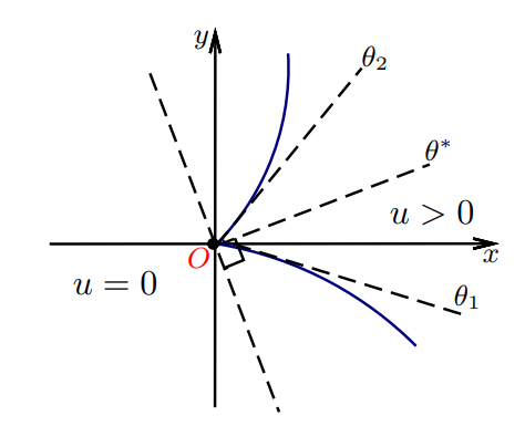
Figure 10. Singular profile for Type 3 stagnation point

Remark 1.12.

In Case 3, the external force f vanishes at the origin, and then we can not define the direction of the force at the stagnation point. However, due to introducing a potential function, we can formulate that it solves a Tschebysheff equation. And then it gives the homogeneity of the blow-up limits and the deflection angle $\theta_{2}-\theta_{1}$ of the free boundary near the origin.

The present paper is built up as follows. In Section 2, based on Weiss’ monotonicity formula, we investigate three different possible singular profiles close to the Type 1 , Type 2 and Type 3 stagnation points respectively, that must be corner wave, cusp or flat profile. By analyzing the local cusp geometry at stagnation points, it is proven that cusp profile does not exist in Section 3, while flat profile is eliminated using the idea of perturbation in frequency formula in Section 4. Section 5 contains asymptotic behavior of the free boundary approaching stagnation points.

2. Monotonicity formula and blow-up limits

In this section, we will investigate the possible blow-up limits and weighted densities near three types of stagnation points respectively.

2.1. Case 1. Type 1 stagnation point

For Subcase 1.1, the gradient function on the free boundary is

$$h_{0}(x,y)=(-x)^{\alpha}(-y)^{\beta},\,\,\alpha\geq 0,\beta\geq 1.$$ (2.1)

We work out the explicit blow-up limits by means of the monotonicity formula. Monotonicity formula is important for the study of this paper, which is used to determine that the blow-up limit is a homogeneous function. This concept has been confirmed in [23]. The difference between the monotonicity formula for Case 1 and 2 and which in [23] is that there will be an extra perturbation term. The previous monotonicity formula is therefore not directly applicable. The derivative of the Weiss adjusted boundary energy we obtained is a nonnegative term plus a perturbation term. Let us first introduce $\delta:=\min\{X_{0},\rm{dist}$$(X_{0},\partial\Omega)/2\}$ throughout the paper.

Lemma 2.1.

(Monotonicity formula). Let $u$ be a weak solution of the free boundary problem (1.3) and for any $r\in(0,\delta)$, recalling (1.6),

$$M_{1}(r)=r^{-2-\beta}\int_{B_{r}(X_{0})}\left(\left|\nabla u\right|^{2}+(-x)^{\alpha}(-y)^{\beta}\chi_{\{u>0\}}\right)dX-\dfrac{\beta+2}{2}r^{-3-\beta}\int_{\partial B_{r}(X_{0})}u^{2}d\mathcal{H}^{1}.$$

Then, the function $M_{1}(r)$ is differentiable almost everywhere on $(0,\delta)$ and for almost every $r\in(0,\delta)$, we have

$$\dfrac{dM_{1}(r)}{dr}=2r^{-2-\beta}\int_{\partial B_{r}(X_{0})}\left(\nabla u\cdot\nu-\frac{\beta+2}{2}\frac{u}{r}\right)^{2}d\mathcal{H}^{1}+h_{1}(r),$$ (2.2)

where $\nu$ is the unit outer normal vector to the boundary and

$$h_{1}(r)=r^{-3-\beta}\int_{B_{r}(X_{0})}\alpha(-x)^{\alpha-1}(x_{0}-x)(-y)^{\beta}\chi_{\{u>0\}}dX.$$ (2.3)

Proof.

For convenience, $M_{1}(r)$ can be written as $M_{1}(r)=I_{1}(r)+J_{1}(r)$, where

$$I_{1}(r)= r^{-2-\beta}\int_{B_{r}(X_{0})}\left(\left|\nabla u\right|^{2}+(-x)^{\alpha}(-y)^{\beta}\chi_{\{u>0\}}\right)dX,$$

and

$$J_{1}(r)= r^{-3-\beta}\int_{\partial B_{r}(X_{0})}u^{2}d\mathcal{H}^{1}.$$

Differentiating $J_{1}(r)$ with respect to $r$ gives

$$\dfrac{dJ_{1}(r)}{dr}=(-3-\beta)r^{-4-\beta}\int_{\partial B_{r}(X_{0})}u^{2}d\mathcal{H}^{1}+r^{-3-\beta}\dfrac{d}{dr}\left(\int_{\partial B_{r}(X_{0})}u^{2}d\mathcal{H}^{1}\right),$$

substituting the second term on the right side of the last equation by scaling properties, $J^{\prime}_{1}(r)$ can be derived as follows

$$\frac{dJ_{1}(r)}{dr}=-(\beta+2)r^{-4-\beta}\int_{\partial B_{r}(X_{0})}u^{2}d\mathcal{H}^{1}+2r^{-3-\beta}\int_{\partial B_{r}(X_{0})}u\nabla u\cdot\nu d\mathcal{H}^{1}.$$ (2.4)

A similar computation as Theorem 3.5 in [23] gives rise to

$$\frac{dI_{1}(r)}{dr}=2r^{-2-\beta}\int_{\partial B_{r}(X_{0})}(\nabla u\cdot\nu)^{2}d\mathcal{H}^{1}-(2+\beta)r^{-3-\beta}\int_{\partial B_{r}(X_{0})}u\nabla u\cdot\nu d\mathcal{H}^{1}+h_{1}(r).$$ (2.5)

Together with (2.4), the proof is concluded. ∎

Remark 2.2.

It is important to recall that (1.5) implies that for any small $r$,

$$u(x)\leq C_{1}(-x)^{\frac{\alpha}{2}}(-y)^{\frac{\beta}{2}+1}$$ (2.6)

holds locally in $B_{r}(X_{0})$ for a positive constant $C_{1}$.

In view of (2.6), it is easy to check that $u_{m}\in W^{1,2}(B_{r}(X_{0}))$, hence, there exists a weakly convergent subsequence of $u_{m}$ in $W^{1,2}(B_{r}(X_{0}))$.

Lemma 2.3.

Let $u$ be a weak solution of the free boundary problem (1.3) satisfying (2.6) and $r_{m}\rightarrow 0+$ as $m\rightarrow\infty$, then the limit

$$\lim\limits_{m\rightarrow\infty}M_{1}(r_{m})$$

exists and is finite.

Proof.

Since $h_{1}(r)$ is integrable with respect to $r$ when $r\in(0,\delta)$, the function $\int_{0}^{r}h_{1}(s)ds$ is well-defined. By virtue of the monotonicity formula, we have

$$\dfrac{d}{dr}\left(M_{1}(r)-\int_{0}^{r}h_{1}(s)ds\right)\geq 0.$$

As stated in Theorem 1.1 of [22], $\lim\limits_{r\rightarrow 0+}\left(M_{1}(r)-\int_{0}^{r}h_{1}(s)ds\right)$ exists. On account of (2.6) and $u(X_{0})=0$, one has the existence of $M_{1}(0+)$. ∎

With the help of the preceding two lemmas, we now use the Weiss’ monotonicity formula to prove that the homogeneity of blow-up limit $u_{0}$, the higher compactness of blow-up sequence $u_{m}$ and the specific expression of $M_{1}(0+)$, the results are given in Lemma 2.4.

Lemma 2.4.

Let $u$ be a weak solution of the free boundary problem (1.3) with (2.6), and $r_{m}$ be a vanishing sequence of positive real numbers such that the blow-up sequence $u_{m}(X)=r_{m}^{-\frac{\beta+2}{2}}u(X_{0}+r_{m}X)$ converges weakly in $W_{\text{loc}}^{1,2}(\mathbb{R}^{2})$ to a blow-up limit $u_{0}$. Then

(i) $u_{0}(X)$ is a homogeneous function of $\frac{\beta+2}{2}$ degree;

(ii) there is a subsequence $u_{m}$ converges strongly to $u_{0}$ in $W_{\text{loc}}^{1,2}(\mathbb{R}^{2})$ as $m\rightarrow\infty$;

(iii) the weighted density is

$$M_{1}(0+)=(-x_{0})^{\alpha}\lim\limits_{m\rightarrow\infty}\int_{B_{1}}(y_{-})^{\beta}\chi_{\{u_{m}>0\}}dX.$$ (2.7)

Proof.

(i) For each $0<\rho<\sigma<\delta$ integrating (2.2) in the monotonicity formula with respect to $r$ on $(r_{m}\rho,r_{m}\sigma)$, we obtain

$$2\int_{B_{\sigma}\backslash B_{\rho}}|X|^{-\beta-4}\left(\nabla u_{m}(X)\cdot X-\dfrac{\beta+2}{2}u_{m}(X)\right)^{2}dX$$

$$= M_{1}(r_{m}\sigma)-M_{1}(r_{m}\rho)-\int_{r_{m}\rho}^{r_{m}\sigma}h_{1}(r)dr\rightarrow 0,\,\,\,\text{as}\,\,m\rightarrow\infty,$$

the above equation is derived also due to the fact that $h_{1}(r)$ is integrable with respect to $r$ in $(0,\delta)$.

It follows from the fact $u_{m}(X)\rightarrow u_{0}(X)$ weakly in $W^{1,2}_{\text{loc}}(\mathbb{R}^{2})$ that

$$\nabla u_{0}(X)\cdot X-\dfrac{\beta+2}{2}u_{0}(X)=0\,\,\,\text{a.e. in}\,\,\mathbb{R}^{2},$$ (2.8)

the homogeneity we wanted can be easily derived from (2.8).

(ii) We start by noticing that by the Bernstein estimate and the weak convergence of $u_{m}$, $u_{m}\in W^{1,\infty}(B_{r})$, for each $0<r<+\infty$. The strong convergence of the blow-up sequence in $L^{2}_{\text{loc}}(\mathbb{R}^{2})$ can be derived by the compact embedding $W^{1,\infty}(U)\hookrightarrow L^{\infty}(U)\hookrightarrow L^{2}(U)$, where $U$ is a bounded domain of $\mathbb{R}^{2}$.

Now, we claim that

$$\limsup\limits_{m\rightarrow\infty}\left\|\nabla u_{m}\right\|_{L^{2}(U)}\leq\left\|\nabla u_{0}\right\|_{L^{2}(U)}.$$ (2.9)

In fact, for each $m$, the blow-up sequence $u_{m}$ satisfies

$$\Delta u_{m}=0\,\,\,\,\,\text{in}\,B_{\delta/r_{m}}\cap\{u_{m}>0\}.$$ (2.10)

Taking $m\rightarrow\infty$, $u_{m}$ converges locally uniformly to $u_{0}$ in $\{u_{m}>0\}$ gives that

$$\Delta u_{0}=0\,\,\,\text{in }\,\{u_{0}>0\}.$$ (2.11)

Besides, we give the following definition by the idea of mollification, for any $\varepsilon>0$,

$$\operatorname{max}\left(u_{m}-\varepsilon,0\right)^{1+\varepsilon}=\begin{cases}(u_{m}-\varepsilon)^{1+\varepsilon}\,\,&u_{m}>\varepsilon,\\ 0&0\leq u_{m}<\varepsilon.\end{cases}$$

Noticing that $\operatorname{supp}\left(\operatorname{max}\left(u_{m}-\varepsilon,0\right)^{1+\varepsilon}\right)\subset\{u_{m}>0\}$, we have

$$\int_{\mathbb{R}^{2}}\nabla u_{m}\cdot\nabla\operatorname{max}\left(u_{m}-\varepsilon,0\right)^{1+\varepsilon}\eta dX=-\int_{\mathbb{R}^{2}}u_{m}\nabla\operatorname{max}\left(u_{m}-\varepsilon,0\right)^{1+\varepsilon}\cdot\nabla\eta d\mathcal{H}^{1},$$ (2.12)

for any $\eta\in C_{0}^{1}(\mathbb{R}^{2})$.

Let $\varepsilon\rightarrow 0$, together with the convergence of $u_{m}$, we obtain

$$\lim\limits_{m\rightarrow\infty}\int_{\mathbb{R}^{2}}|\nabla u_{m}|^{2}\eta dX=\int_{\mathbb{R}^{2}}|\nabla u_{0}|^{2}\eta dX,$$ (2.13)

the claim (2.9) immediately follows from the equation (2.13). Eventually, by means of Proposition 3.32 in [7], we can show that there exists a subsequence still relabeled by $u_{m}$ such that $\nabla u_{m}\rightarrow\nabla u_{0}$ strongly in $L^{2}_{\text{loc}}(\mathbb{R}^{2}).$

(iii) For any $m\rightarrow\infty$, $r_{m}$ is an infinitesimal sequence of positive real numbers, we calculate the limit of $M_{1}(r_{m})$ directly,

$$M_{1}(0+)=\lim\limits_{m\rightarrow\infty} M_{1}(r_{m})$$ (2.14)

$$=\lim\limits_{m\rightarrow\infty} \bigg{[}\int_{B_{1}}\left(|\nabla u_{m}|^{2}+(-x_{0})^{\alpha}(y_{-})^{\beta}\chi_{\{u_{m}>0\}}\right)dX-\dfrac{\beta+2}{2}\int_{\partial B_{1}}u_{m}^{2}d\mathcal{H}^{1}\bigg{]},$$

$$=(-x_{0} )^{\alpha}\lim\limits_{m\rightarrow\infty}\int_{B_{1}}(y_{-})^{\beta}\chi_{\{u_{m}>0\}}dX+\int_{B_{1}}|\nabla u_{0}|^{2}dX-\dfrac{\beta+2}{2}\int_{\partial B_{1}}u_{0}^{2}d\mathcal{H}^{1},$$

the last equality being a consequence of the strong convergence and trace theorem.

On the other hand, the homogeneity of $u_{0}$ suggests that

$$\int_{B_{1}}|\nabla u_{0}|^{2}dX=\dfrac{\beta+2}{2}\int_{\partial B_{1}}u_{0}^{2}d\mathcal{H}^{1}.$$ (2.15)

Accordingly, this together with (2.15) and (2.14) implies the result (2.7). ∎

It is apparent from (2.7) that the result of $M_{1}(0+)$ is decided by the limit of characteristic function $\lim\limits_{m\rightarrow\infty}\chi_{\{u_{m}>0\}}$. In the next proposition, we deduce that $\lim\limits_{m\rightarrow\infty}\chi_{\{u_{m}>0\}}$ must be

$$\chi_{\left\{-\frac{\beta+4}{2(\beta+2)}\pi<\theta<-\frac{\beta}{2(\beta+2)}\pi\right\}}\,\,\text{or}\,\,0\,\,\text{or}\,\,1,$$

thereby giving all possible exact forms of the blow-up limits and the corresponding densities for Subcase 1.1.

Proposition 2.5.

Let $u$ be a weak solution of the free boundary problem (1.3) satisfying (2.6). Then we may decompose $S^{u}$ into the disjoint union $S^{u}=S^{u}_{1,\text{corner}}\cup S^{u}_{1,\text{cusp}}\cup S^{u}_{1,\text{flat}}$, we define

(i) $S^{u}_{1,\text{corner}}=\left\{X=(x_{0},0)\in S^{u}\Big{|}M_{1}(0+)=(-x_{0})^{\alpha}\int_{B_{1}\bigcap\left\{-\frac{\beta+4}{2(\beta+2)}\pi<\theta<-\frac{\beta}{2(\beta+2)}\pi\right\}}(y_{-})^{\beta}dX\right\}$, and the corresponding blow-up limit is

$$u_{0}(r\cos\theta,\sin\theta)=\dfrac{2(-x_{0})^{\frac{\alpha}{2}}}{\beta+2}r^{\frac{\beta+2}{2}}\cos^{\frac{\beta}{2}}\left(\dfrac{\pi}{\beta+2}\right)\cos\left(\dfrac{\beta+2}{2}\theta+\dfrac{\beta+2}{4}\pi\right)\chi_{\left\{-\frac{\beta+4}{2(\beta+2)}\pi<\theta<-\frac{\beta}{2(\beta+2)}\pi\right\}},$$

the corner wave profile see Fig. 6(a);

(ii) $S^{u}_{1,\text{cusp}}=\left\{X=(x_{0},0)\in S^{u}|M_{1}(0+)=0\right\}$, and the corresponding blow-up limit is

$$u_{0}=0,$$

the cusp wave profile see Fig. 11(a) and (b);

(iii) $S^{u}_{1,\text{flat}}=\left\{X=(x_{0},0)\in S^{u}\big{|}M_{1}(0+)=(-x_{0})^{\alpha}\int_{B_{1}}(y_{-})^{\beta}dX\right\}$, and the corresponding blow-up limit is

$$u_{0}=0,$$

the flat wave profile see Fig. 11.(c).

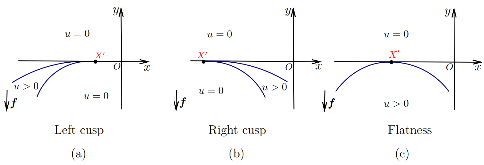
Figure 11. Cusp point and flat point

Proof.

Setting $\phi=(\phi_{1},\phi_{2})\in C^{1}_{0}(\mathbb{R}^{2},\mathbb{R}^{2})$ as the test function in (1.4), then we obtain

$$0= \int_{\Omega_{m}}|\nabla u_{m}|^{2}\operatorname{div}\phi dZ-2\int_{\Omega_{m}}\nabla u_{m}D\phi\nabla u_{m}dZ+\int_{\Omega_{m}}(-x_{0}-r_{m}z_{1})^{\alpha}(z_{2-})^{\beta}\operatorname{div}\phi\chi_{\{u_{m}>0\}}dZ$$

$$+\int_{\Omega_{m}}\big{(}-\alpha(-x_{0}-r_{m}z_{1})^{\alpha-1}r_{m}(z_{2-})^{\beta}\phi_{1}-\beta(-x_{0}-r_{m}z_{1})^{\alpha}(z_{2-})^{\beta-1}\phi_{2}\big{)}\chi_{\{u_{m}>0\}}dZ,$$

where $\Omega_{m}=\{Z=(z_{1},z_{2})|X_{0}+r_{m}Z\in\Omega\}$. Passing to the limit as $m\rightarrow\infty$, we get that

$$0= \int_{\mathbb{R}^{2}}\left(|\nabla u_{0}|^{2}\operatorname{div}\phi-2\nabla u_{0}D\phi\nabla u_{0}\right)dX+\int_{\mathbb{R}^{2}}(-x_{0})^{\alpha}(y_{-})^{\beta}\operatorname{div}\phi\chi_{0}dX$$ (2.16)

$$+\int_{\mathbb{R}^{2}}\big{(}-\beta(-x_{0})^{\alpha}(y_{-})^{\beta-1}\phi_{2}\big{)}\chi_{0}dX,$$

where $\chi_{0}$ is the strong $L^{1}_{\text{loc}}$-limit of $\chi_{\{u_{m}>0\}}$ along a subsequence. The values of the function $\chi_{0}$ are almost everywhere in $\{0,1\}$, and the locally uniform convergence of $u_{m}$ to $u_{0}$ implies that

$$\chi_{0}=1\text{ in }\{u_{0}>0\}.$$ (2.17)

Suppose first that the set $\{u_{0}>0\}$ is empty, then (2.16) tells us that in the interior of $\{u_{0}=0\}$,

$$(-x_{0})^{\alpha}\int_{\mathbb{R}^{2}}\operatorname{div}\big{(}(y_{-})^{\beta}\phi\big{)}\chi_{0}dX=0.$$ (2.18)

It follows from (2.18) that $\chi_{0}$ is a constant in each connected component of the interior of $\{u_{0}=0\}\cap\{X=(x,y)|y<0\}$, and we denote it as $\overline{\chi}_{0}$. Thus it is sufficient to show that when the blow-up limit $u_{0}\equiv 0$, the corresponding densities are

$$M_{1}(0+)=0\,\,\text{or}\,\,M_{1}(0+)=(-x_{0})^{\alpha}\int_{B_{1}}(y_{-})^{\beta}dX.$$

Consider now the second case when $\{u_{0}>0\}$ is not an empty set.

Together with the homogeneity of blow-up limit $u_{0}$, we can write the harmonic function $u_{0}$ in polar coordinates, we have that

$$u_{0}(r,\theta)=C_{0}r^{\frac{\beta+2}{2}}\cos\left(\dfrac{\beta+2}{2}\theta+\varphi_{0}\right),$$ (2.19)

where $C_{0}>0$ and $\varphi_{0}$ are constants to be determined. Each connected component of $\{u_{0}>0\}$ is thereby a cone with vertex at the origin and an angle of $\frac{2\pi}{\beta+2}$.

If we choose any point $Z\in\partial\{u_{0}>0\}\backslash\{(0,0)\}$, there is a sufficiently small constant $\omega$ such that the outer normal to $\partial\{u_{0}>0\}$ is a constant vector $\nu(Z)$ in $B_{\omega}(Z)\cap\partial\{u_{0}>0\}$. Setting $\phi(X):=\eta(X)\nu(Z)$ for any $\eta\in C_{0}^{1}(B_{\omega}(Z))$ as the test function in (2.16), combining with (2.17), we get that

$$\int_{B_{\omega}(Z)\cap\partial\{u_{0}>0\}}|\nabla u_{0}|^{2}\eta d\mathcal{H}^{1}=(-x_{0})^{\alpha}\int_{B_{\omega}(Z)\cap\partial\{u_{0}>0\}}(y_{-})^{\beta}(1-\overline{\chi_{0}})\eta d\mathcal{H}^{1}.$$ (2.20)

Indeed, it follows from the Hopf’s lemma that $|\nabla u_{0}|\neq 0$ on $B_{\omega}(Z)\cap\partial\{u_{0}>0\}$, from which and (2.20), we deduce

$$|\nabla u_{0}|^{2}=(-x_{0})^{\alpha}(y_{-})^{\beta}\,\,\text{on}\,\,\partial\{u_{0}>0\}.$$ (2.21)

Now, we will establish the possible explicit form of $u_{0}$ with the help of (2.21). Applying (2.19) in (2.21), we have that

$$\dfrac{(\beta+2)^{2}}{4}C_{0}^{2}=(-x_{0})^{\alpha}\left(\left(\sin\theta\right)_{-}\right)^{\beta},$$ (2.22)

which holds on both boundaries of the cone.

We denote the boundaries of the cone intersect $x$-axis at angles $\theta_{1}$ and $\theta_{2}$ respectively, and $\theta_{1}<\theta_{2}$. Besides, $x_{0}<0$ is mentioned previously, then the following relationships hold,

$\sin\theta_{1}=\sin\theta_{2}<0$ and $\theta_{2}-\theta_{1}=\dfrac{2\pi}{\beta+2}$.

Thus one has that $\theta_{1}=-\frac{\pi}{\beta+2}-\frac{\pi}{2}=-\frac{\beta+4}{2(\beta+2)}\pi$ and $\theta_{2}=\frac{\pi}{\beta+2}-\frac{\pi}{2}=-\frac{\beta}{2(\beta+2)}\pi$, which yields that

$$C_{0}=\dfrac{2(-x_{0})^{\frac{\alpha}{2}}}{\beta+2}\cos^{\frac{\beta}{2}}\left(\dfrac{\pi}{\beta+2}\right).$$

Moreover, it follows from the boundary condition that $\varphi_{0}=\frac{\beta+2}{4}\pi+k\pi$, for some integer $k$. Noticing that $\varphi_{0}=\frac{\beta+2}{4}\pi$ and $u_{0}(r,\theta)\geq 0$ for $k=0$. Finally, the expression of $u_{0}$ is

$$u_{0}(r,\theta)=\dfrac{2(-x_{0})^{\frac{\alpha}{2}}}{\beta+2}r^{\frac{\beta+2}{2}}\cos^{\frac{\beta}{2}}\left(\dfrac{\pi}{\beta+2}\right)\cos\left(\dfrac{\beta+2}{2}\theta+\dfrac{\beta+2}{4}\pi\right)\chi_{\left\{-\frac{\beta+4}{2(\beta+2)}\pi<\theta<-\frac{\beta}{2(\beta+2)}\pi\right\}},$$

and the corresponding weighted density is

$$M_{1}(0+)=(-x_{0})^{\alpha}\int_{B_{1}\bigcap\left\{-\frac{\beta+4}{2(\beta+2)}\pi<\theta<-\frac{\beta}{2(\beta+2)}\pi\right\}}(y_{-})^{\beta}dX,$$

which concludes the proof of Proposition 2.5. ∎

Reasoning as above, we just need to substitute the equation (2.1) as follows respectively,

$h_{0}(x,y)=x^{\alpha}y^{\beta}\,\,$ for Subscase 1.2;

$h_{0}(x,y)=(-x)^{\alpha}y^{\beta}\,\,$ for Subscase 1.3;

$h_{0}(x,y)=x^{\alpha}(-y)^{\beta}\,\,$ for Subscase 1.4.

The pertinent results have been stated in Theorem 1.1 without proof.

2.2. Case 2. Type 2 stagnation point

We consider the gradient function in Subcase 2.1 as

$$h_{0}(x,y)=(-x)^{\alpha}(-y)^{\beta},\,\,\alpha\geq 1,\beta\geq 0.$$ (2.23)

Similar to what we did in the proof of Subcase 1.1, we can obtain the following conclusions of Subcase 2.1.

Remark 2.6.

Note that (1.5) implies that for any small $r$,

$$u(x)\leq C_{2}(-x)^{\frac{\alpha}{2}+1}(-y)^{\frac{\beta}{2}}$$ (2.24)

locally in $B_{r}(X_{0})$ for a positive constant $C_{2}$.

Proposition 2.7.

Suppose that (2.24) holds, and let $u$ be a weak solution of the free boundary problem (1.3), then the following conclusions hold.

(i) (Monotonicity formula) for any $r\in(0,\delta)$, recalling (1.6), the Weiss adjusted boundary energy is

$$M_{2}(r)=r^{-2-\alpha}\int_{B_{r}(X_{0})}\left(\left|\nabla u\right|^{2}+(-x)^{\alpha}(-y)^{\beta}\chi_{\{u>0\}}\right)dX-\dfrac{\alpha+2}{2}r^{-3-\alpha}\int_{\partial B_{r}(X_{0})}u^{2}d\mathcal{H}^{1}.$$ (2.25)

Then the function $M_{2}(r)$ is differentiable almost everywhere on $(0,\delta)$ and for a.e. $r\in(0,\delta)$, we have

$$\dfrac{dM_{2}(r)}{dr}=2r^{-2-\alpha}\int_{\partial B_{r}(X_{0})}\left(\nabla u\cdot\nu-\frac{\alpha+2}{2}\frac{u}{r}\right)^{2}d\mathcal{H}^{1}+h_{2}(r),$$

where

$$h_{2}(r)=r^{-3-\alpha}\int_{B_{r}(X_{0})}\beta(-x)^{\alpha}(y_{0}-y)(-y)^{\beta-1}\chi_{\{u>0\}}dX.$$

(ii) (Blow-up sequence and blow-up limit) For $m\rightarrow\infty$, let $r_{m}$ be a vanishing sequence of positive real numbers such that the blow-up sequence $u_{m}(X)=r_{m}^{-\frac{\alpha+2}{2}}u(X_{0}+r_{m}X)$ converges weakly in $W_{\text{loc}}^{1,2}(\mathbb{R}^{2})$ to a blow-up limit $u_{0}$. Then $u_{0}$ is a homogeneous function of $\frac{\alpha+2}{2}$ degree. Moreover, $u_{m}$ converges strongly to $u_{0}$ in $W_{\text{loc}}^{1,2}(\mathbb{R}^{2})$.

(iii) (Weighted density) The limit $M_{2}(0+)$ exists and the weighted density is

$$M_{2}(0+)=(-y_{0})^{\beta}\lim\limits_{m\rightarrow\infty}\int_{B_{1}}(x_{-})^{\alpha}\chi_{\{u_{m}>0\}}dX.$$

(iv) (Possible singular profiles) The set of corner wave stagnation point is

$$S^{u}_{2,\text{corner}}=\left\{X=(0,y_{0})\in S^{u}\bigg{|}M_{2}(0+)=(-y_{0})^{\beta}\int_{B_{1}\bigcap\left\{\frac{\alpha+1}{\alpha+2}\pi<\theta<\frac{\alpha+3}{\alpha+2}\pi\right\}}(x_{-})^{\alpha}dX\right\},$$

and the corresponding blow-up limit is

$$u_{0}(r,\theta)=\dfrac{2(-y_{0})^{\frac{\beta}{2}}}{\alpha+2}r^{\frac{\alpha+2}{2}}\cos^{\frac{\alpha}{2}}\left(\frac{\alpha+1}{\alpha+2}\pi\right)\cos\left(\dfrac{\alpha+2}{2}\theta+\dfrac{2-\alpha}{2}\pi\right)\chi_{\left\{\frac{\alpha+1}{\alpha+2}\pi<\theta<\frac{\alpha+3}{\alpha+2}\pi\right\}}.$$

The set of cusp stagnation point and flat stagnation point are

$$S^{u}_{2,\text{cusp}}=\left\{X=(0,y_{0})\in S^{u}\big{|}M_{2}(0+)=0\right\}$$

and

$$S^{u}_{2,\text{flat}}=\left\{X=(0,y_{0})\in S^{u}\Big{|}M_{2}(0+)=(-y_{0})^{\beta}\int_{B_{1}}(x_{-})^{\alpha}dX\right\}$$

respectively, and the corresponding blow-up limit of the both is

$$u_{0}=0.$$

The corner wave profile see Fig. 8(a), the cusp wave profile see Fig. 12(a) and (b), the flat wave profile see Fig. 12(c).

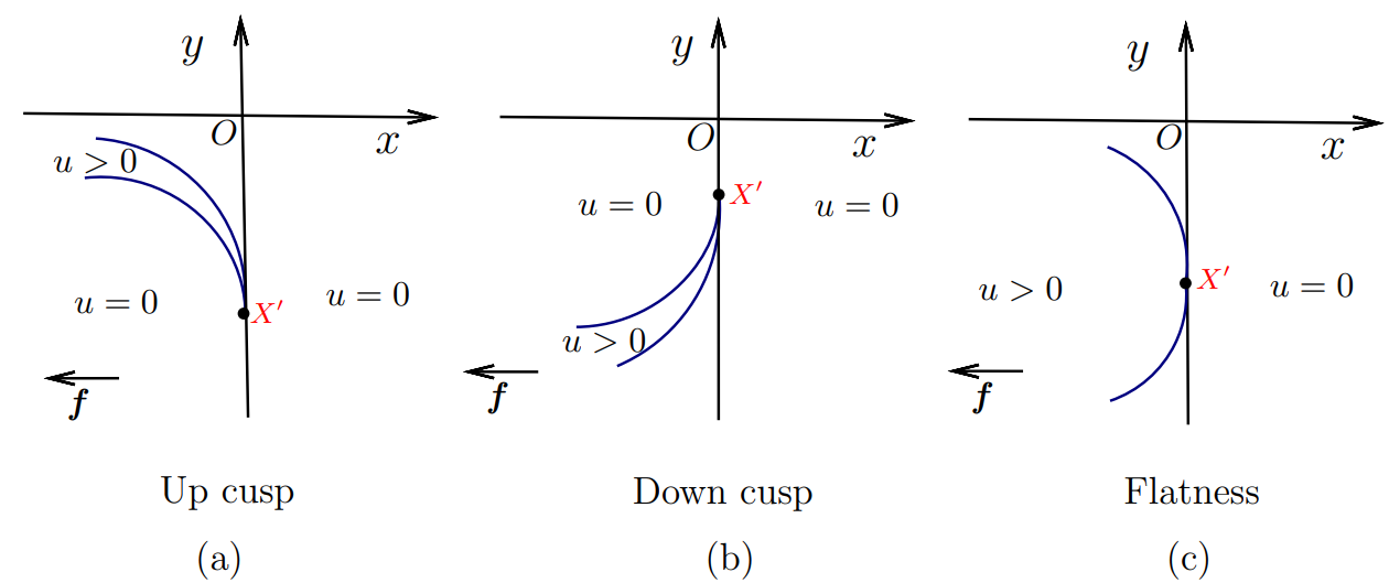
Figure 12. Cusp point and flat point

2.3. Case 3. Type 3 stagnation point

In the subsection, we would like to study the singular profile near Type 3 stagnation point $X_{0}=(0,0)$. Similar to what we did in Lemma 2.1, the derivative of the Weiss functional for the Type 3 stagnation point will be concluded firstly.

Lemma 2.8.

(Monotonicity formula). Let $u$ be a weak solution of (1.3) and for any $r\in(0,\delta)$, recalling (1.6) we have that

$$M_{3}(r)= r^{-2-\alpha-\beta}\int_{B_{r}(X_{0})}\left(\left|\nabla u\right|^{2}+|x|^{\alpha}|y|^{\beta}\chi_{\{u>0\}}\right)dX-\dfrac{\alpha+\beta+2}{2}r^{-3-\alpha-\beta}\int_{\partial B_{r}(X_{0})}u^{2}d\mathcal{H}^{1}.$$

Then, the function $M_{3}(r)$ is differentiable almost everywhere on $(0,\delta)$ and for almost everywhere $r\in(0,\delta)$, we have

$$\dfrac{dM_{3}(r)}{dr}=2r^{-2-\alpha-\beta}\int_{\partial B_{r}(X_{0})}\left(\nabla u\cdot\nu-\frac{\alpha+\beta+2}{2}\frac{u}{r}\right)^{2}d\mathcal{H}^{1}.$$

Remark 2.9.

It is important to recall that the decay rate (1.5) implies that for any small $r$,

$$u(x)\leq C_{3}\left(|x|^{\frac{\alpha}{2}+1}|y|^{\frac{\beta}{2}}+|x|^{\frac{\alpha}{2}}|y|^{\frac{\beta}{2}+1}\right)$$ (2.26)

holds locally in $B_{r}(X_{0})$ for a positive constant $C_{3}$.

Lemma 2.10.

Suppose that with (2.26) holds, and let $u$ be a weak solution of the free boundary problem (1.3). For $m\rightarrow\infty$, let $r_{m}$ be a vanishing sequence of positive real numbers.

(i) (Blow-up sequence and blow-up limit) Suppose that the blow-up sequence $u_{m}(X)=r_{m}^{-\frac{\alpha+\beta+2}{2}}u(X_{0}+r_{m}X)$ converges weakly in $W_{\text{loc}}^{1,2}(\mathbb{R}^{2})$ to a blow-up limit $u_{0}$. Then $u_{0}$ is a homogeneous function of $\frac{\alpha+\beta+2}{2}$ degree and $u_{m}$ converges strongly to $u_{0}$ in $W_{\text{loc}}^{1,2}(\mathbb{R}^{2})$.

(ii) (Weighted density) The limit $M_{3}(0+)$ exists and the weighted density is

$$M_{3}(0+)=\lim\limits_{m\rightarrow\infty}\int_{B_{1}}|x|^{\alpha}|y|^{\beta}\chi_{\{u_{m}>0\}}dX.$$

Proof.

The existence of $M_{3}(0+)$ follows directly from that $M^{\prime}_{3}(r)\geq 0$ and $|M_{3}(r)|$ is bounded. The same method of Lemma 2.4 can be used to verify the rest conclusion of this lemma, and we omit the proof here. ∎

Proposition 2.11.

Let $u$ be a weak solution of the free boundary problem (1.3) satisfying (2.26), then we have the following conclusion:

The set of corner wave stagnation point is

$$S^{u}_{3,\text{corner}}=\left\{X\in S^{u}\bigg{|}M_{3}(0+)=\int_{B_{1}\cap\left\{\theta_{1}<\theta<\theta_{2}\right\}}|x|^{\alpha}|y|^{\beta}dX\right\},$$

where $\theta_{1}$ and $\theta_{2}$ are the angles of the asymptotic direction of free boundaries intersect $x$-axis near the origin with $\theta_{1}<\theta_{2}$, $\theta_{2}-\theta_{1}=\frac{2\pi}{\alpha+\beta+2}$ and the boundary condition of blow-up limit. For each pair of $\theta_{1}$ and $\theta_{2}$, the corresponding blow-up limit is

$$u_{0}(r,\theta)=\dfrac{2|\cos\theta_{1}|^{\frac{\alpha}{2}}|\sin\theta_{1}|^{\frac{\beta}{2}}}{\alpha+\beta+2}r^{\frac{\alpha+\beta+2}{2}}\cos\left(\frac{\alpha+\beta+2}{2}\theta+\arcsin\left|\cos\left(\frac{\alpha+\beta+2}{2}\theta_{1}\right)\right|\right)\chi_{\left\{\theta_{1}<\theta<\theta_{2}\right\}}.$$

The set of cusp stagnation point and flat stagnation point are

$$S^{u}_{3,\text{cusp}}=\left\{X\in S^{u}\big{|}M_{3}(0+)=0\right\}$$

and

$$S^{u}_{3,\text{flat}}=\left\{X\in S^{u}\Big{|}M_{3}(0+)=\int_{B_{1}}|x|^{\alpha}|y|^{\beta}dX\right\}$$

respectively, and the corresponding blow-up limit of the both is

$$u_{0}=0.$$

The corner wave profile see Fig. 10, the cusp profile see Fig. 13(a) and (b), and flat profile see Fig. 13(c).

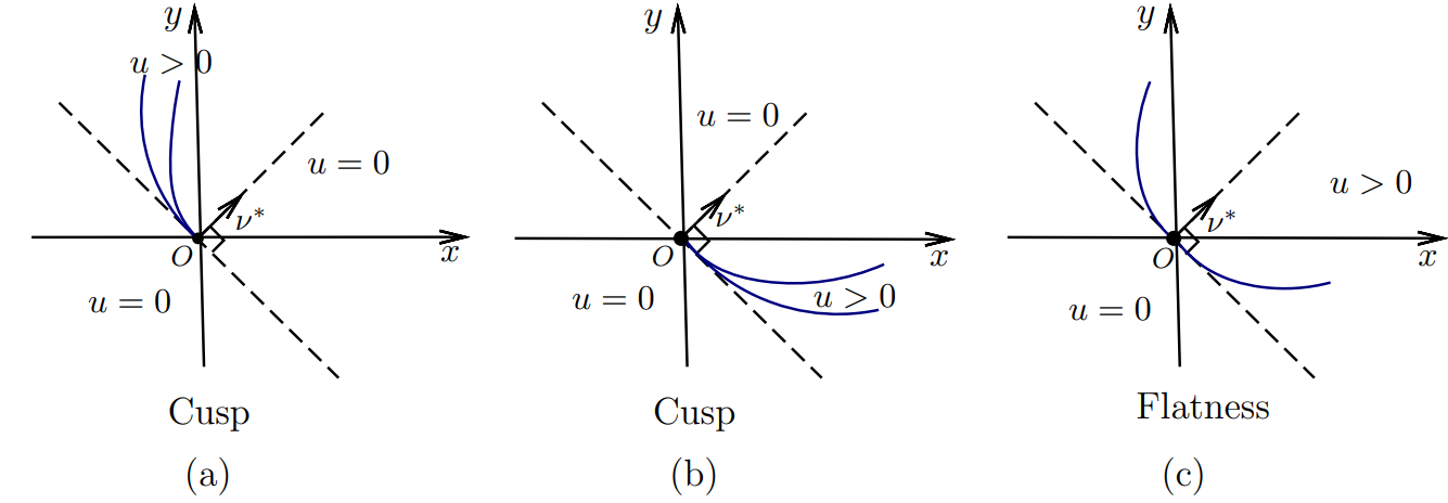
Figure 13. Cusp point and flat point

Proof.

By suitable modification to the proof of Proposition 2.5, we can confirm the case of cusp and flatness. Furthermore, under the assumption that $\{u_{0}>0\}$ is non-empty,

$$u_{0}(r,\theta)=r^{\frac{\alpha+\beta+2}{2}}C_{0}\cos\left(\dfrac{\alpha+\beta+2}{2}\theta+\varphi_{0}\right)$$ (2.27)

holds, and each connected component of $\{u_{0}>0\}$ is a cone with vertex at the origin and an angle of $\frac{2\pi}{\alpha+\beta+2}$. It follows from (2.27) and the boundary condition that

$$\dfrac{(\alpha+\beta+2)^{2}}{4}C_{0}^{2}=|\cos\theta|^{\alpha}|\sin\theta|^{\beta},$$ (2.28)

which holds on both boundaries of the cone.

In each connected component of $\{u_{0}>0\}$, we introduce a velocity potential $\phi_{0}$ defined by

$\dfrac{\partial\phi_{0}}{\partial x}=-\dfrac{\partial u_{0}}{\partial y}$ and $\dfrac{\partial\phi_{0}}{\partial y}=\dfrac{\partial u_{0}}{\partial x}.$

Let $\psi_{0}(x_{1},x_{2},x_{3})=\phi_{0}\left(\sqrt{x_{1}^{2}+x_{2}^{2}},x_{3}\right)$, through a direct calculation, we have in $\{u_{0}>0\}$,

$$\Delta\psi_{0}=\dfrac{1}{x}\dfrac{\partial}{\partial x}\left(x\dfrac{\partial\phi_{0}}{\partial x}\right)+\dfrac{1}{x^{2}}\dfrac{\partial^{2}\phi_{0}}{\partial\gamma^{2}}+\dfrac{\partial^{2}\phi_{0}}{\partial y^{2}}=\dfrac{1}{x}\dfrac{\partial\phi_{0}}{\partial x},$$ (2.29)

where $x=\sqrt{x_{1}^{2}+x_{2}^{2}},y=x_{3},\gamma=\arctan\frac{x_{2}}{x_{1}}$. This implies that $\psi_{0}(x_{1},x_{2},x_{3})$ in $\{u_{0}>0\}$ satisfies

$$\dfrac{1}{r^{2}}\dfrac{\partial}{\partial r}\left(r^{2}\dfrac{\partial\psi_{0}}{\partial r}\right)+\dfrac{1}{r^{2}\cos\theta}\dfrac{\partial}{\partial\theta}\left(\cos\theta\dfrac{\partial\psi_{0}}{\partial\theta}\right)-\dfrac{1}{r}\dfrac{\partial\phi_{0}}{\partial r}+\dfrac{\sin\theta}{r^{2}\cos\theta}\dfrac{\partial\phi_{0}}{\partial\theta}=0,$$ (2.30)

where $r=\sqrt{x_{1}^{2}+x_{2}^{2}+x_{3}^{2}}$ and $\theta=\arctan\frac{x_{3}}{\sqrt{x_{1}^{2}+x_{2}^{2}}}$.

Since $\phi_{0}(r\cos\theta,r\sin\theta)$ is a homogeneous function of $\frac{\alpha+\beta+2}{2}$ degree, we can rewrite that

$$\phi_{0}(r\cos\theta,r\sin\theta)=r^{\frac{\alpha+\beta+2}{2}}g(\cos\theta),$$ (2.31)

$g(\cos\theta)$ is a smooth function with respect to $\cos\theta$ to be determined later. For easy of notations, setting $z=\cos\theta$. Inserting (2.31) into (2.30), we compute that $g(z)$ satisfies the following Tschebysheff equation in $\{u_{0}>0\}$,

$$(1-z^{2})g^{\prime\prime}(z)-zg^{\prime}(z)+\frac{(\alpha+\beta+2)^{2}}{4}g(z)=0.$$

The solution of the Tschebysheff equation (see in [29]) is

$$g(z)=a\cos\left(\frac{\alpha+\beta+2}{2}\theta\right)+b\sin\left(\frac{\alpha+\beta+2}{2}\theta\right),$$

where $a$ and $b$ are the coefficients to be determined.

Noticing that $|\nabla u_{0}|^{2}=|\nabla\phi_{0}|^{2}$, we have

$$\begin{cases}\left(\frac{\alpha+\beta+2}{2}\right)^{2}(a^{2}+b^{2})=|\cos\theta_{1}|^{\alpha}|\sin\theta_{1}|^{\beta},\\ \left(\frac{\alpha+\beta+2}{2}\right)^{2}(a^{2}+b^{2})=|\cos\theta_{2}|^{\alpha}|\sin\theta_{2}|^{\beta}.\end{cases}$$ (2.32)

It follows from the homogeneity of $u_{0}$ that

$$u_{0}(r\cos\theta,r\sin\theta)=r^{\frac{\alpha+\beta+2}{2}}f(\cos\theta),$$ (2.33)

where $f(\cos\theta)$ is a smooth function with respect to $\cos\theta$ to be determined later, which together with (2.31) gives that

$$\dfrac{\partial\phi_{0}}{\partial\theta}=r\dfrac{\partial u_{0}}{\partial r},$$

the relationship of $f(\cos\theta)$ and $g(\cos\theta)$ can be easily derived as follows

$$\dfrac{dg(\cos\theta)}{d\theta}=\frac{\alpha+\beta+2}{2}f(\cos\theta).$$

Moreover, recalling the free boundary condition of $u_{0}$,

$$u_{0}(r\cos\theta_{i},\sin\theta_{i})=r^{\frac{\alpha+\beta+2}{2}}f(\cos\theta_{i})=0,\,i=1,2,$$

thus we deduce that

$$\dfrac{dg(\cos\theta)}{d\theta}\bigg{|}_{\theta=\theta_{i}}=0,$$

a directly computation yields that

$$a\sin\left(\frac{\alpha+\beta+2}{2}\theta_{i}\right)-b\cos\left(\frac{\alpha+\beta+2}{2}\theta_{i}\right)=0,\,\text{for}\,i=1,2.$$ (2.34)

All in all, $\theta_{i}$ solves the equations (2.32) and (2.34). For simplicity of presentation, we define $A=\frac{2\pi}{\alpha+\beta+2}$ and the function $f(\tan\theta)$ as

$$f(\tan\theta)=\left|\cos A-\tan\theta\sin A\right|^{\alpha}\left|\cos A+\dfrac{1}{\tan\theta}\sin A\right|^{\beta}-1,$$ (2.35)

solving for $\theta_{1}$ and $\theta_{2}$ in (2.32) and (2.34) is equivalent to solving for the zeros of the function $f$. By conveniently denoting $s(\theta)=\tan\theta$, we now write $f(\tan\theta)$ as

$$f(s)=\left|\cos A-s\sin A\right|^{\alpha}\left|\cos A+\dfrac{1}{s}\sin A\right|^{\beta}-1.$$

Obviously, $f(s)\rightarrow+\infty$ if $s\rightarrow 0$ or $\infty$. Besides $f(\frac{1}{\tan A})=-1$ and $f(-\tan A)=-1$. The zeros of function (2.35) is proved via the monotonic properties of $f(s)$. The situation of the zeros is related to the size of $\alpha$ and $\beta$. Here we illustrate the case of $\alpha\geq\beta$ as an example, and the result of $\alpha<\beta$ is analogous. We can summarize the results as follows.

If $0<\tan A\leq\frac{2\sqrt{\alpha\beta}}{\alpha-\beta}$, the graph of $f(s)$ is illustrated in Fig. 14(a), if $\tan A>\frac{2\sqrt{\alpha\beta}}{\alpha-\beta}$, the graph of $f(s)$ is illustrated in Fig. 14(b).

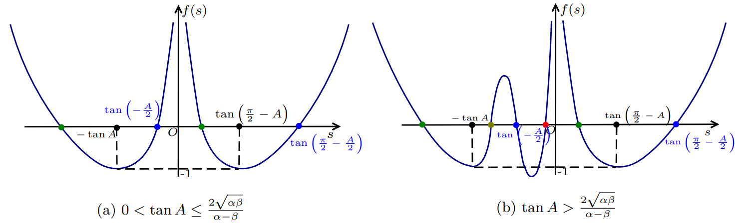
Figure 14. The graph of $f(s)$ for $\alpha\geq\beta$

The zeros of $f(s)$ can imply the solutions of $\theta_{1}$ in (2.32). If $0<\tan A\leq\frac{2\sqrt{\alpha\beta}}{\alpha-\beta}$, there are eight pairs of solutions $(\theta_{1},\theta_{2})$. Furthermore, four pairs of solutions are symmetric about the coordinate axes, see Fig. 15, the other four pairs of them are non-symmetric, see Fig. 16.

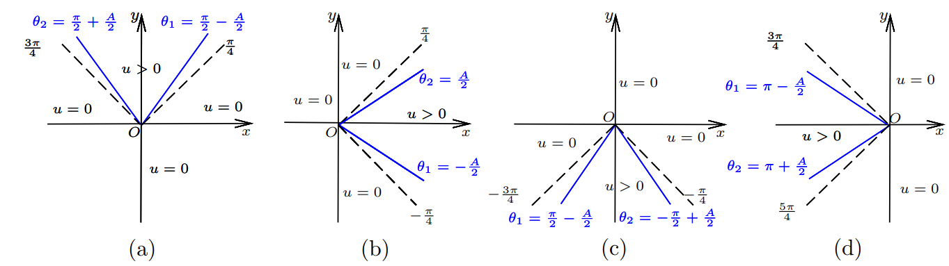
Figure 15. The symmetric solutions for $0<\tan A\leq\frac{2\sqrt{\alpha\beta}}{\alpha-\beta}$ ($\alpha\geq\beta$)

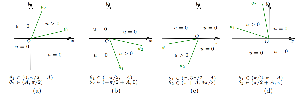
Figure 16. The non-symmetric solutions for $0<\tan A\leq\frac{2\sqrt{\alpha\beta}}{\alpha-\beta}$ ($\alpha\geq\beta$)

If $\tan A>\frac{2\sqrt{\alpha\beta}}{\alpha-\beta}$, except for the solutions mentioned in Fig. 15 and Fig. 16, there are other four pairs of non-symmetric solutions, see Fig. 17.

‘

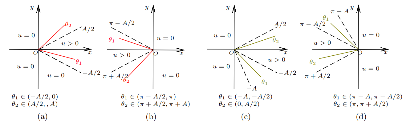
Figure 17. Additional non-symmetric solutions for $\tan A>\frac{2\sqrt{\alpha\beta}}{\alpha-\beta}$ ($\alpha\geq\beta$)

Naturally, we can decide the coefficients $C_{0}$ and $\varphi_{0}$ by $a$ and $b$. Based on the above analysis, the expression of $u_{0}$ and the corresponding weighted density can be concluded. ∎

Remark 2.12.

Since the force is degenerate at $X_{0}=(0,0)$, the direction of f does not exist. Asymptotic directions of the free boundary can not be determined in this situation.

3. Non-existence of cusp profile

In the next lemma, we can show that, for the degenerate weighted density case $M_{i}(r)\equiv 0$ ($i=1,2,3)$, the cusp phenomenon does not happen. Without loss of generality, we pick the most complex Case 3 for the proof, as two variables are degenerate for this case. Case 1 and Case 2 are similar, and we omit it here.

Proposition 3.1.

For Type 3 stagnation point $X_{0}=(0,0)$, let $u$ be a weak solution of (1.3) and suppose that

$$|\nabla u|^{2}\leq|x|^{\alpha}|y|^{\beta}$$ (3.1)

in $B_{r}(O)$, for some small $r>0$. Then the set of $S^{u}_{3,\text{cusp}}$ is empty.

Proof.

Suppose towards a contradiction that $X_{0}=(0,0)\in S^{u}_{3,\text{cusp}}$, and the blow-up sequence $u_{m}(X)=r_{m}^{-\frac{\alpha+\beta+2}{2}}u(r_{m}X)$ converges weakly in $W_{\text{loc}}^{1,2}(\mathbb{R}^{2})$ to a blow-up limit $u_{0}$. The corresponding blow-up limit of $M_{3}(0+)=0$ is $u_{0}\equiv 0$ in $\mathbb{R}^{2}$, as reasoning above, we have that

$$\Delta u_{m}(B_{2})\rightarrow 0,\,\,\text{as}\,m\rightarrow\infty,$$ (3.2)

and

$$\Delta u_{m}(B_{2})\geq\int_{B_{2}\cap\partial_{red}\{u_{m}>0\}}\sqrt{|x|^{\alpha}|y|^{\beta}}d\mathcal{H}^{1},$$ (3.3)

where $\Delta u$ is a non-negative Radon measure in $\Omega$ and $\partial_{red}$ is the reduced boundary.

Moreover, we denote that $A=(-1,1)\times(0,1)$. Based on the maximum principle, there is at least one connected component $V_{m}$ of $\{u_{m}>0\}$, such that for any $m$, $V_{m}$ contains the origin and some points of $\partial A$.

At first, we define

$$\zeta_{m}(x,y)=\max\left\{|x|^{\alpha}|y|^{\beta}|X=(x,y)\in V_{m}\cap\partial A\right\}.$$

As $m\rightarrow\infty$, if $\zeta_{m}(x,y)$ is bounded away from zero, a contradiction to (3.2) and (3.3) is an easy consequence of the convergence. In fact, if not, when $\zeta_{m}(x,y)$ converge to zero, we now calculate $\Delta u_{m}$ in the region $V_{m}\cap A$,

$$0= \Delta u_{m}(V_{m}\cap A)$$

$$= \int_{\partial V_{m}\cap A}\nabla u_{m}\cdot\nu d\mathcal{H}^{1}+\int_{V_{m}\cap\partial A}\nabla u_{m}\cdot\nu d\mathcal{H}^{1},$$

together with the boundary condition and (3.1), we get that

$$0\leq\int_{\partial V_{m}\cap A}\left(-\sqrt{|x|^{\alpha}|y|^{\beta}}\right)d\mathcal{H}^{1}+\int_{V_{m}\cap\partial A}\sqrt{|x|^{\alpha}|y|^{\beta}}d\mathcal{H}^{1}.$$

The last inequality is a contradiction, which concludes the proof. ∎

4. Non-existence of flat profile

In this section, we give the detailed analysis for the non-existence of flatness. The main method we used is the frequency formula, this is a classical result, which is first studied by F. Almgren in [1]. However, the gradient function we study here has two variables, the direct frequency formula in [23] does not work. It is worth to know that we exclude flat point by perturbation, which is referred in [25]. Accordingly, we have to use remainder term in monotonicity formula to perturbate the frequency, more details will be shown in this section. Unless otherwise specified, we take $u$ be a weak solution of (1.3).

At first, we investigate Subcase 1.1, recalling that

$$S^{u}_{1,\text{flat}}:=\left\{X_{0}=(x_{0},0)\in S^{u}\Big{|}M_{1}(0+)=(-x_{0})^{\alpha}\int_{B_{1}}(y_{-})^{\beta}dX\right\}$$

as the set of flat stagnation points in Subcase 1.1.

Remark 4.1.

We have to point out that the set $S^{u}_{1,\text{flat}}$ is closed due to the fact that the function $M_{1}(0+)$ is upper semicontinuous about $X$.

Lemma 4.2.

Let $X_{0}$ be a point of the closed set $S^{u}_{1,\text{flat}}$, and for some $r_{0}\in(0,\delta)$ sufficiently small, we define for $r\in(0,r_{0})$

$$D(r)=r\dfrac{\int_{B_{r}(X_{0})}|\nabla u|^{2}dX}{\int_{\partial B_{r}(X_{0})}u^{2}d\mathcal{H}^{1}},$$

and

$$V(r)=r\dfrac{\int_{B_{r}(X_{0})}\left[\left(-x_{0}\right)^{\alpha}\left(y_{-}\right)^{\beta}-(-x)^{\alpha}(-y)^{\beta}\chi_{\{u>0\}}\right]dX+r^{2+\beta}\int_{0}^{r}h_{1}(t)dt}{\int_{\partial B_{r}(X_{0})}u^{2}d\mathcal{H}^{1}}.$$ (4.1)

And we define the frequency function

$$H(r)=D(r)-V(r).$$

Then some properties of $V(r)$ and the frequency function $H(r)$ hold as follows:

(i) the frequency function satisfies $H(r)\geq\frac{\beta}{2}+1$ for all $r\in(0,r_{0})$;

(ii) the function $\frac{1}{r}V^{2}(r)$ is integrable with respect to $r$ when $r\in(0,r_{0})$;

(iii) the limit of the frequency function $\lim\limits_{r\rightarrow 0+}H(r)$ exists, denoted as $H(0+)$. Obviously, we know that $H(0+)\geq\frac{\beta}{2}+1$.

Proof.

We first write $H(r)$ as

$$H(r)=\dfrac{I_{*}(r)-(-x_{0})^{\alpha}\int_{B_{1}}(y_{-})^{\beta}dX}{J_{1}(r)},$$ (4.2)

where

$$I_{*}(r)=I_{1}(r)-\int_{0}^{r}h_{1}(t)dt.$$

In order to get the conclusion (i), it is equivalent to the following inequality

$$I_{*}(r)-\left(\dfrac{\beta}{2}+1\right)J_{1}(r)-r^{-2-\beta}(-x_{0})^{\alpha}\int_{B_{r}(X_{0})}(y_{-})^{\beta}dX\geq 0,$$

which follows from the direct calculation,

$$I_{*}(r)-\left(\dfrac{\beta}{2}+1\right)J_{1}(r)-r^{-2-\beta}(-x_{0})^{\alpha}\int_{B_{r}(X_{0})}(y_{-})^{\beta}dX$$ (4.3)

$$= M_{1}(r)-M_{1}(0+)-\int_{0}^{r}h_{1}(t)dt$$

$$= \int_{0}^{r}\dfrac{dM_{1}(t)}{dt}dt-\int_{0}^{r}h_{1}(t)dt$$

$$\geq 0.$$

The above equation holds since monotonicity formula (2.2) shows us that the third term of (4.3) is a perfect square term. Hence, we obtain the statement (i).

Next together with (2.4), we calculate the derivative of $H(r)$ with (4.2),

$$\dfrac{dH(r)}{dr}= \dfrac{I^{\prime}_{1}(r)-h_{1}(r)}{J_{1}(r)}-\left(D(r)-V(r)\right)\cdot\dfrac{J^{\prime}_{1}(r)}{J_{1}(r)}$$

$$= \dfrac{2r^{-2-\beta}\int_{\partial B_{r}(X_{0})}(\nabla u\cdot\nu)^{2}d\mathcal{H}^{1}-(\beta+2)r^{-3-\beta}\int_{\partial B_{r}(X_{0})}u\nabla u\cdot\nu d\mathcal{H}^{1}+h_{1}(r)-h_{1}(r)}{r^{-3-\beta}\int_{\partial B_{r}(X_{0})}u^{2}d\mathcal{H}^{1}}$$

$$-\left(D(r)-V(r)\right)\cdot\dfrac{J^{\prime}_{1}(r)}{J_{1}(r)}$$

$$= \dfrac{2r^{-2-\beta}\int_{\partial B_{r}(X_{0})}(\nabla u\cdot\nu)^{2}d\mathcal{H}^{1}-(\beta+2)r^{-3-\beta}\int_{\partial B_{r}(X_{0})}u\nabla u\cdot\nu d\mathcal{H}^{1}}{r^{-3-\beta}\int_{\partial B_{r}(X_{0})}u^{2}d\mathcal{H}^{1}}$$

$$-\left(D(r)-V(r)\right)\dfrac{2r^{-3-\beta}\int_{\partial B_{r}(X_{0})}u\nabla u\cdot\nu d\mathcal{H}^{1}-(\beta+2)r^{-4-\beta}\int_{\partial B_{r}(X_{0})}u^{2}d\mathcal{H}^{1}}{r^{-3-\beta}\int_{\partial B_{r}(X_{0})}u^{2}d\mathcal{H}^{1}}.$$

By rearranging the above equation, it follows that

$$\dfrac{dH(r)}{dr}=\dfrac{2}{r}\Bigg{[} \dfrac{\int_{\partial B_{r}(X_{0})}\left(r(\nabla u\cdot\nu)-D(r)u\right)^{2}d\mathcal{H}^{1}}{\int_{\partial B_{r}(X_{0})}u^{2}d\mathcal{H}^{1}}+V^{2}(r)+V(r)\left(H(r)-\left(\dfrac{\beta}{2}+1\right)\right)\Bigg{]}$$ (4.4)

$$=\dfrac{2}{r}\Bigg{[} \dfrac{\int_{\partial B_{r}(X_{0})}\left(r(\nabla u\cdot\nu)-H(r)u\right)^{2}d\mathcal{H}^{1}}{\int_{\partial B_{r}(X_{0})}u^{2}d\mathcal{H}^{1}}+V(r)\left(H(r)-\left(\dfrac{\beta}{2}+1\right)\right)\Bigg{]}.$$

Moreover, $V(r)$ can be rewritten as

$$V(r)=\dfrac{V_{1}(r)+V_{2}(r)}{\int_{\partial B_{r}(X_{0})}u^{2}d\mathcal{H}^{1}},$$

where

$$V_{1}(r)=\left(-x_{0}\right)^{\alpha}r\int_{B_{r}(X_{0})}\left(y_{-}\right)^{\beta}(1-\chi_{\{u>0\}})dX,$$ (4.5)

and

$$V_{2}(r)=r\int_{B_{r}(X_{0})}\left[\left(-x_{0}\right)^{\alpha}-(-x)^{\alpha}\right](-y)^{\beta}\chi_{\{u>0\}}dX+r^{3+\beta}\int_{0}^{r}h_{1}(t)dt.$$ (4.6)

Obviously, we infer form (4.5), (4.6) and (2.3) that

$V_{1}(r)\leq C\left(r^{\beta+3}\right)$ and $V_{2}(r)\leq C\left(r^{\beta+4}\right)$,

where $C$ is some constant. Therefore as $r<r_{0}$, it follows from $V_{1}(r)\geq 0$ that $V(r)\geq 0$.

In other word, (4.4) also implies that $\frac{2}{r}V^{2}(r)\leq H^{\prime}(r),$ the conclusion (ii) and (iii) can be derived together with the fact that $H(r)$ is bounded below as $r\rightarrow 0+$, which concludes the proof. ∎

The frequency formula allows us passing to blow-up limit.

Proposition 4.3.

Let $X_{0}\in S^{u}_{1,\text{flat}}$ and suppose that the weak solution satisfies (2.6). Then

(i) $\lim\limits_{r\rightarrow 0+}V(r)=0$ and $\lim\limits_{r\rightarrow 0+}D(r)=H(0+)$;

(ii) for any infinitesimal sequence $r_{m}$, where $m\rightarrow\infty$, we define $v_{m}$ as

$$v_{m}(X):=\dfrac{u(X_{0}+r_{m}X)}{\sqrt{r_{m}^{-1}\int_{\partial B_{r_{m}}(X^{{}^{\prime}})}u^{2}d\mathcal{H}^{1}}},$$ (4.7)

the sequence $v_{m}$ is bounded in $W^{1,2}(B_{1})$;

(iii) suppose that the sequence $v_{m}$ defined in (4.7) converges weakly in $W^{1,2}(B_{1})$ to a blow-up limit $v_{0}$, then the function $v_{0}$ is continuous and is a homogeneous function of $H(0+)$ degree in $B_{1}$, and satisfies $v_{0}\geq 0$ in $B_{1}$, $v_{0}\equiv 0$ in $B_{1}^{+}$ where $B_{1}^{+}=B_{1}\cap\{X=(x,y)|y\geq 0\}$, and $\int_{\partial B_{1}}v^{2}_{0}d\mathcal{H}^{1}=1$.

Proof.

First, we claim for any sequence $r_{m}\rightarrow 0+$ and every $0<\rho<\sigma<1$, the sequence $v_{m}$ defined in (4.7) satisfies,

$$\int_{B_{\sigma}\backslash B_{\rho}}|X|^{-4-\beta}\left(\nabla v_{m}\cdot X-H(0+)v_{m}\right)^{2}dX\,\rightarrow 0,\,\text{ as }m\rightarrow\infty.$$ (4.8)

Indeed, for any such $\rho$ and $\sigma$, and every $m$ such that $r_{m}<\delta$. As $m\rightarrow\infty$, it follows from (4.4) that,

$$\int_{\rho}^{\sigma}\dfrac{2}{s}\left[\dfrac{\int_{\partial B_{s}}\left(s\nabla v_{m}\cdot\nu-H(sr_{m})v_{m}\right)^{2}d\mathcal{H}^{1}}{\int_{\partial B_{s}}v^{2}_{m}d\mathcal{H}^{1}}\right]ds\leq H(r_{m}\sigma)-H(r_{m}\rho)\rightarrow 0.$$ (4.9)

Firstly, we want to show that

$$J_{1}(r)=r^{-3-\beta}\int_{\partial B_{r}(X_{0})}u^{2}(X)d\mathcal{H}^{1}\,\,\,\,\text{is non-decreasing.}$$ (4.10)

Together with the monotonicity formula and (4.3), we acquire

$$\dfrac{dJ_{1}(r)}{dr}= 2r^{-1}\bigg{(}I_{1}(r)-\int_{0}^{r}h_{1}(t)dt-\left(\dfrac{\beta}{2}+1\right)J_{1}(r)-(-x_{0})^{\alpha}\int_{B_{1}}(y_{-})^{\beta}dX$$

$$-r^{-2-\beta}\int_{B_{r}(X_{0})}\left(-x\right)^{\alpha}\left(-y\right)^{\beta}\chi_{\{u>0\}}dX+\int_{0}^{r}h_{1}(t)dt+(-x_{0})^{\alpha}\int_{B_{1}}(y_{-})^{\beta}dX\bigg{)}$$

$$\geq 2r^{-3-\beta}\bigg{(}\left(-x_{0}\right)^{\alpha}\int_{B_{r}(X_{0})}\left(y_{-}\right)^{\beta}(1-\chi_{\{u>0\}})dX$$

$$+r^{2+\beta}\int_{0}^{r}h_{1}(t)dt+\int_{B_{r}(X_{0})}\left[\left(-x_{0}\right)^{\alpha}-(-x)^{\alpha}\right](-y)^{\beta}\chi_{\{u>0\}}dX\bigg{)}.$$

It follows from the similar reason as $V(r)\geq 0$ in Lemma 4.2 that we have $J^{\prime}_{1}(r)\geq 0$.

Now note that, for every $s\in(\rho,\sigma)\subset(0,1)$ and $m$ as before. Recalling the definition of $v_{m}$, we calculate the integration of $v^{2}_{m}$ on $\partial B_{s}$, we have

$$\int_{\partial B_{s}}v^{2}_{m}d\mathcal{H}^{1} =\dfrac{\int_{\partial B_{r_{m}s}(X_{0})}u^{2}(X)d\mathcal{H}^{1}}{\int_{\partial B_{r_{m}}(X_{0})}u^{2}(X)d\mathcal{H}^{1}}$$

$$=\dfrac{(r_{m}s)^{-3-\beta}\int_{\partial B_{r_{m}s}(X_{0})}u^{2}(X)d\mathcal{H}^{1}}{r_{m}^{-3-\beta}\int_{\partial B_{r_{m}}(X_{0})}u^{2}(X)d\mathcal{H}^{1}}s^{3+\beta}.$$

Since $J_{1}(r)$ is non-decreasing, it follows that

$$\int_{\partial B_{s}}v^{2}_{m}d\mathcal{H}^{1}\leq s^{3+\beta}.$$ (4.11)

Combining with (4.9), as $m\rightarrow\infty$, we have

$$\int_{\rho}^{\sigma}\dfrac{2}{s}s^{-3-\beta}\int_{\partial B_{s}}\left(s\nabla v_{m}\cdot\nu-H(sr_{m})v_{m}\right)^{2}d\mathcal{H}^{1}ds\rightarrow 0.$$ (4.12)

Thus (4.8) follows from the fact (4.12).

Next, we use the claim (4.8) to give the proof of the results in this proposition.

For the result (i), we argue by contradiction. Suppose that $V(s_{m})\nrightarrow 0$, where $s_{m}$ is a vanishing sequence of positive constants. It follows from the fact that $\frac{1}{r}V^{2}(r)$ is integrable with respect to $r\in[s_{m},2s_{m}]$, hence, that the minimum of $V(r)$ converges to zero as $m\rightarrow\infty$.

Without loss of generality, we may assume that $r_{m}$ is a sequence such that $r_{m}\in[s_{m},2s_{m}]$ and $V(r_{m})\rightarrow 0$ as $m\rightarrow\infty$. In view of the existence of the frequency function $H(0+)$, $D(r_{m})$ is bounded as $r_{m}\rightarrow 0+$. We now calculate $D(r_{m})$ by scaling,

$$D(r_{m})=\int_{B_{1}}|\nabla v_{m}|^{2}dX.$$ (4.13)

Thus (ii) holds and there exists $v_{0}\in W^{1,2}(B_{1})$ as the weak limit of $v_{m}$ up to a subsequence. Together with the trace theorem $W^{1,2}(B_{1})\hookrightarrow L^{2}(\partial B_{1})$, we have

$v_{m}\rightarrow v_{0}$ strongly in $L^{2}(\partial B_{1})$.

The conclusion (iii) now follows by a direct calculation of $\int_{\partial B_{1}}|v_{m}|^{2}dX=1$ and (4.8). It remains to show that (i) holds. Substituting $s_{m}$ into the definition of $V(r)$ for $r$,

$$V(s_{m})$$ (4.14)

$$= \dfrac{s_{m}^{-2-\beta}\left[\int_{B_{s_{m}}(X_{0})}\left(-x_{0}\right)^{\alpha}\left(y_{-}\right)^{\beta}(1-\chi_{\{u>0\}})+\left[\left(-x_{0}\right)^{\alpha}-(-x)^{\alpha}\right](-y)^{\beta}\chi_{\{u>0\}}dX+s_{m}^{2+\beta}\int_{0}^{s_{m}}h_{1}(t)dt\right]}{s_{m}^{-3-\beta}\int_{\partial B_{s_{m}}(X_{0})}u^{2}d\mathcal{H}^{1}}$$

$$\leq \dfrac{s_{m}^{-2-\beta}\int_{\partial B_{r_{m}}(X_{0})}u^{2}d\mathcal{H}^{1}}{\left(\frac{r_{m}}{2}\right)^{-2-\beta}\int_{\partial B_{\frac{r_{m}}{2}}(X_{0})}u^{2}d\mathcal{H}^{1}}V(r_{m}).$$

Due to the definition of $v_{m}$ in (4.7), we can substitute

$$\int_{\partial B_{\frac{r_{m}}{2}}(X_{0})}u^{2}d\mathcal{H}^{1}$$

with

$$\int_{\partial B_{\frac{1}{2}}}v_{m}^{2}d\mathcal{H}^{1}\int_{\partial B_{r_{m}}(X_{0})}u^{2}d\mathcal{H}^{1}$$

in inequality (4.14), that is

$$V(s_{m})\leq\left(\dfrac{r_{m}}{2s_{m}}\right)^{2+\beta}\dfrac{V(r_{m})}{\int_{\partial B_{\frac{1}{2}}}v_{m}^{2}d\mathcal{H}^{1}}\leq\dfrac{V(r_{m})}{\int_{\partial B_{\frac{1}{2}}}v_{m}^{2}d\mathcal{H}^{1}}.$$ (4.15)

Next, we claim that

$$\int_{\partial B_{\frac{1}{2}}}v_{m}^{2}d\mathcal{H}^{1}\rightarrow\int_{\partial B_{\frac{1}{2}}}v_{0}^{2}d\mathcal{H}^{1}>0.$$ (4.16)

Suppose that the claim (4.16) doesn’t hold, i.e. $\int_{\partial B_{\frac{1}{2}}}v_{0}^{2}d\mathcal{H}^{1}=0$, this means $v_{0}=0$ holds almost everywhere on $\partial B_{\frac{1}{2}}$. While the homogeneity of $v_{0}$ deduces that

$$v_{0}(X)=(2|X|)^{H(0+)}v_{0}\left(\frac{X}{2|X|}\right),$$

$v_{0}=0$ holds almost everywhere on $\partial B_{1}$, this is a contradiction to $\int_{\partial B_{1}}v_{0}^{2}d\mathcal{H}^{1}=1$.

Thus the fact that inequality (4.15) and $V(r_{m})\rightarrow 0$ implies $V(s_{m})\rightarrow 0$, which leads to a contradiction to the fact that $V(s_{m})$ is bounded away from $0$. Therefore we have $V(r)\rightarrow 0$ and $D(r)\rightarrow H(0+)$ as $r\rightarrow 0+$. We now conclude the proof of Proposition 4.3. ∎

Next proposition allows us to preserve weak solution in the blow-up limit at stagnation points and show that $S^{u}_{\text{flat}}$ is an empty set.

Proposition 4.4.

Let $X_{0}\in S^{u}_{1,\text{flat}}$ and $r_{m}$ be a vanishing sequence of positive real numbers such that the sequence $v_{m}$ defined in (4.7) converging weakly in $W^{1,2}(B_{1})$ to a limit $v_{0}$. Then

(i) there is a subsequence $v_{m}$ converging strongly to $v_{0}$ in $W^{1,2}_{\text{loc}}(B_{1}\backslash\{0,0\})$, and $v_{0}$ is continuous in $B_{1}$. Moreover, $\Delta v_{0}$ is a non-negative Radon measure and $v_{0}\Delta v_{0}=0$ holds in the sense of Radon measure in $B_{1}$;

(ii) at each point $X_{0}$ of the set $S^{u}_{1,\text{flat}}$ there exists an integer $N(X_{0})\geq\frac{\beta}{2}+1$ such that

$$H(0+)=N(X_{0}),$$

and $\text{as}\,\,r\rightarrow 0+$,

$$\dfrac{u(X_{0}+rX)}{\sqrt{r^{-1}\int_{\partial B_{r}(X^{{}^{\prime}})}u^{2}d\mathcal{H}^{1}}}\rightarrow\dfrac{\rho^{N(X_{0})}\big{|}\sin(N(X_{0})\min\{\max\{\theta,\pi\},2\pi\})\big{|}}{\left(\int_{0}^{\pi}\sin^{2}(N(X_{0})\theta)d\theta\right)^{\frac{1}{2}}},$$ (4.17)

that is

$$v_{0}=\begin{cases}0\,\,\,&\theta\leq\pi,\\ \dfrac{\rho^{N(X_{0})}|\sin(N(X_{0})\theta)|}{\left(\int_{0}^{\pi}\sin^{2}(N(X_{0})\theta)d\theta\right)^{\frac{1}{2}}}\,\,\,\,&\pi<\theta<2\pi,\\ 0&\theta\geq 2\pi,\end{cases}$$

where $X=(\rho\cos\theta,\rho\sin\theta)$.

Proof.

This is a standard result which following the proof of Theorem 9.1 and Theorem 10.1 in [23], therefore we omit the detail of the proof here.

(i) Based on Theorem 1.1 and 3.1 in [15] and Theorem 8.17 in [17], we can obtain that $v_{m}\rightarrow v_{0}$ strongly in $W^{1,2}_{\text{loc}}(B_{1}\backslash\{0,0\})$. As a consequence of the strong convergence, we obtain that $v_{0}\Delta v_{0}=0$ in the sense of Radon measure in $B_{1}$.

(ii) Due to the homogeneity of $v_{0}$ and $\Delta v_{0}=0$ in $\{v_{0}>0\}$,

$$v_{0}(\rho,\theta)=\begin{cases}\dfrac{\rho^{N(X_{0})}|\sin(N(X_{0})\theta)|}{\sqrt{\int_{0}^{\pi}\sin^{2}\left(N(X_{0})\theta\right)d\theta}}\,\,&\theta\in(\theta_{1},\theta_{2}),\\ 0&\theta\notin(\theta_{1},\theta_{2}).\end{cases}$$

In addition, for $v_{0}\equiv 0$ in $\mathbb{R}^{2}\backslash\{X=(x,y)|y\geq 0\}$, $\theta_{1}=\pi$ and $\theta_{2}=2\pi$. ∎

Corollary 4.5.

$S^{u}_{1,\text{flat}}$ is empty.

Proof.

Suppose towards a contradiction that $S^{u}_{1,\text{flat}}\neq\varnothing$, there exists a point $X_{0}\in S^{u}_{1,\text{flat}}$. By Proposition 4.4 (ii), as $r\rightarrow 0+$,

$\dfrac{u(X_{0}+rX)}{\sqrt{r^{-1}\int_{\partial B_{r}(X_{0})}u^{2}d\mathcal{H}^{1}}}\rightarrow\dfrac{\rho^{N(X_{0})}|\sin(N(X_{0})\min\{\max\{\theta,\pi\},2\pi\})|}{\left(\int_{0}^{\pi}\sin^{2}(N(X_{0})\theta)d\theta\right)^{\frac{1}{2}}}$

strongly in $W^{1,2}_{\text{loc}}(B_{1}\backslash\{0,0\})$ and weakly in $W^{1,2}(B_{1})$, where $X=(\rho\cos\theta,\rho\sin\theta).$

In fact, $X_{0}\in S^{u}_{1,\text{flat}}$, then for any ball $\tilde{B}\subset\subset B_{1}\cap\{X=(x,y)|y<0\}$, $v_{m}>0$ in $\tilde{B}$ for sufficiently small $r_{m}$. On the other hand, $v_{0}$ is harmonic in $\tilde{B}$, contradicting (4.17) in view of $N(X_{0})\geq\frac{\beta}{2}+1$. Therefore $S^{u}_{1,\text{flat}}$ is empty. ∎

The proof of Subcase 2.1 can be completed by the same method as employed in Subcase 1.1. However, the proof for Case 3 is slightly different and worth mentioning here. Similarly, we can get the following conclusion. Reviewing the previous definition,

$$S^{u}_{3,\text{flat}}:=\left\{X=(x,y)\in S^{u}\Big{|}M_{3}(0+)=\int_{B_{1}}|x|^{\alpha}|y|^{\beta}dX\right\}$$

as the set of flat stagnation points in Case 3.

Proposition 4.6.

Consider the functions as follows

$$\overline{D}(r)=r\dfrac{\int_{B_{r}}|\nabla u|^{2}dX}{\int_{\partial B_{r}}u^{2}d\mathcal{H}^{1}},$$

$$\overline{V}(r)=r\dfrac{\int_{B_{r}}|x|^{\alpha}|y|^{\beta}\left(1-\chi_{\{u>0\}}\right)dX}{\int_{\partial B_{r}}u^{2}d\mathcal{H}^{1}},$$

and the “frequency” function is

$$\overline{H}(r)=\overline{D}(r)-\overline{V}(r).$$

Then for some $r_{0}\in(0,\delta)$ sufficiently small, the following conclusions hold

(i) $\lim\limits_{r\rightarrow 0+}\overline{V}(r)=0$ and $\lim\limits_{r\rightarrow 0+}\overline{D}(r)=\overline{H}(0+)$;

(ii) for any sequence $r_{m}\rightarrow 0+$ as $m\rightarrow\infty$, the sequence

$$\overline{v}_{m}(x):=\dfrac{u(r_{m}X)}{\sqrt{r_{m}^{-1}\int_{\partial B_{r_{m}}}u^{2}d\mathcal{H}^{1}}}$$ (4.18)

is bounded in $W^{1,2}(B_{1})$;

(iii) suppose that the sequence $\overline{v}_{m}$ in (4.18) converges weakly in $W^{1,2}(B_{1})$ to a blow-up limit $\overline{v}_{0}$, the function $\overline{v}_{0}$ is continuous and a homogeneous function of $\overline{H}(0+)$ degree in $B_{1}$, and satisfies $\overline{v}_{0}\geq 0$ in $B_{1}$, $\overline{v}_{0}\equiv 0$ in $B_{1}\cap\{X|X\cdot\nu^{*}\geq 0\}$, and $\int_{\partial B_{1}}\overline{v}^{2}_{0}d\mathcal{H}^{1}=1$;

(iv) $\overline{v}_{m}$ converges to $\overline{v}_{0}$ strongly in $W^{1,2}_{\text{loc}}(B_{1}\backslash\{0,0\})$, and $\Delta\overline{v}_{0}$ is a non-negative Radon measure satisfying $\overline{v}_{0}\Delta\overline{v}_{0}=0$ in the sense of Radon measure in $B_{1}$;

(v) there exists an integer $\overline{N}(O)\geq\frac{\alpha+\beta}{2}+1$ such that $\overline{H}(0+)=\overline{N}(O),$ and $\text{as}\,\,r\rightarrow 0+$,

$$\dfrac{u(rX)}{\sqrt{r^{-1}\int_{\partial B_{r}}u^{2}d\mathcal{H}^{1}}}\rightarrow\dfrac{\rho^{\overline{N}(O)}|\sin(\overline{N}(O)\min\{\max\{\theta,\theta^{*}-\frac{\pi}{2}\},\theta^{*}+\frac{\pi}{2}\}+\overline{N}(O)(\frac{\pi}{2}+\theta^{*}))|}{\left(\int_{0}^{\pi}\sin^{2}(\overline{N}(O)\theta+\overline{N}(O)(\frac{\pi}{2}-\theta^{*}))d\theta\right)^{\frac{1}{2}}}$$ (4.19)

strongly in $W^{1,2}_{\text{loc}}(B_{1}\backslash(0,0))$ and weakly in $W^{1,2}(B_{1})$, where $X=(\rho\cos\theta,\rho\sin\theta)$.

Corollary 4.7.

$S^{u}_{3,\text{flat}}$ is empty.

Proof.

Suppose towards a contradiction that $S^{u}_{3,\text{flat}}\neq\varnothing$, $X_{0}=(0,0)\in S^{u}_{3,\text{flat}}$. By Proposition 4.6(v), as $r\rightarrow 0+$,

$\dfrac{u(rX)}{\sqrt{r^{-1}\int_{\partial B_{r}}u^{2}d\mathcal{H}^{1}}}\rightarrow\dfrac{\rho^{\overline{N}(O)}|\sin(\overline{N}(O)\min\{\max\{\theta,\theta^{*}-\frac{\pi}{2}\},\theta^{*}+\frac{\pi}{2}\}+\overline{N}(O)(\frac{\pi}{2}+\theta^{*}))|}{\left(\int_{0}^{\pi}\sin^{2}(\overline{N}(O)\theta+\overline{N}(O)(\frac{\pi}{2}-\theta^{*}))d\theta\right)^{\frac{1}{2}}}$

strongly in $W^{1,2}_{\text{loc}}(B_{1}\backslash\{0,0\})$ and weakly in $W^{1,2}(B_{1})$, where $X=(\rho\cos\theta,\rho\sin\theta).$

In fact, for any ball $\tilde{B}\subset\subset B_{1}\cap\{X=(x,y)|X\cdot(\cos\theta^{*},\sin\theta^{*})<0\}$, $\overline{v}_{m}>0$ in $\tilde{B}$ for sufficiently small $r_{m}$, see Fig. 18. On the other hand, $\overline{v}_{0}$ is harmonic in $\tilde{B}$, contradicting (4.19) in view of $\overline{N}(O)\geq\frac{\alpha+\beta}{2}+1$. Hence $S^{u}_{3,\text{flat}}$ is empty.

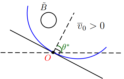
Figure 18. The location of $\tilde{B}$

∎

5. Asymptotic directions of free boundary

Under the assumption that the free boundary is locally an injective curve, we now derive its asymptotic behavior as it approaches a stagnation point. Without loss of generality, taking Subcase 1.1 as an example to prove the conclusion, the proof of other cases can follow from Subcase 1,1, so we omit here.

Proposition 5.1.

Let $u$ be a weak solution of free boundary problem (1.3) satisfying (2.6). Suppose in addition that $\partial\{u>0\}$ is in a neighborhood of $X_{0}$ a continuous injective curve $\sigma=(\sigma_{1}(t),\sigma_{2}(t)):I\rightarrow\mathbb{R}^{2}$ such that $\sigma(0)=X_{0}$, where $I$ is an interval of $\mathbb{R}^{2}$ containing the origin. When

$$M_{1}(0+)=(-x_{0})^{\alpha}\int_{B_{1}\cap\left\{-\frac{\beta+4}{2(\beta+2)}\pi<\theta<-\frac{\beta}{2(\beta+2)}\pi\right\}}(y_{-})^{\beta}dX,$$

then $\sigma_{1}(t)\neq x_{0}$ in $(-s,s)\backslash\{0\}$ and, depending on the parametrization, either

$\lim\limits_{t\rightarrow 0+}\dfrac{\sigma_{2}(t)}{\sigma_{1}(t)-x_{0}}=\tan\left(-\frac{\beta+4}{2(\beta+2)}\pi\right)$ and $\lim\limits_{t\rightarrow 0-}\dfrac{\sigma_{2}(t)}{\sigma_{1}(t)-x_{0}}=\tan\left(-\frac{\beta}{2(\beta+2)}\pi\right),$

or

$\lim\limits_{t\rightarrow 0+}\dfrac{\sigma_{2}(t)}{\sigma_{1}(t)-x_{0}}=\tan\left(-\frac{\beta}{2(\beta+2)}\pi\right)$ and $\lim\limits_{t\rightarrow 0-}\dfrac{\sigma_{2}(t)}{\sigma_{1}(t)-x_{0}}=\tan\left(-\frac{\beta+4}{2(\beta+2)}\pi\right).$

Proof.

We define arg $x$ as the complex argument of $x$ and the sets

$$A_{\pm}:=\left\{\tilde{\theta}\in\left[-\pi,0\right]:\text{there is }\,t_{m}\rightarrow 0\pm\,\text{such that arg}(\sigma(t_{m})-\sigma(0))\rightarrow\tilde{\theta},\,\text{as}\,m\rightarrow\infty\right\}.$$

We claim that

$$A_{\pm}\subset\left\{-\pi,-\frac{\beta+4}{2(\beta+2)}\pi,-\frac{\beta}{2(\beta+2)}\pi,0\right\}.$$

Suppose towards a contradiction that a sequence $\{t_{m}\}$, such that as $m\rightarrow\infty$, $t_{m}\rightarrow 0,$ and

arg$\sigma(t_{m})-$arg$\sigma(0)\rightarrow\tilde{\theta}\in(A_{+}\cup A_{-})\backslash\left\{-\pi,-\frac{\beta+4}{2(\beta+2)}\pi,-\frac{\beta}{2(\beta+2)}\pi,0\right\}$.

Let $r_{m}:=|\sigma(t_{m})-\sigma(0)|$ and

$$u_{m}(X)=\dfrac{u(X_{0}+r_{m}X)}{r_{m}^{\frac{\beta+2}{2}}}.$$

We denote $\tilde{X}=(\cos\tilde{\theta},\sin\tilde{\theta})$, obviously $|\tilde{X}|=1$. And setting lines

$$l_{1}:y=\tan\left(-\frac{\beta}{2(\beta+2)}\pi\right)x,$$

and

$$l_{2}:y=\tan\left(-\frac{\beta+4}{2(\beta+2)}\pi\right)x.$$

For each $\rho>0$, we take a ball $B_{\rho}(\tilde{X})$, which does not intersect $l_{1}$, $l_{2}$ and $x$-axis.

Moreover, we suppose that $X_{m}=\frac{\sigma(t_{m})-\sigma(0)}{r_{m}}$, then

$$u_{m}(X_{m}):=\dfrac{u(X_{0}+\sigma(t_{m})-\sigma(0))}{r_{m}^{\frac{\beta+2}{2}}}=\dfrac{u(\sigma(t_{m}))}{r_{m}^{\frac{\beta+2}{2}}},$$

since $\sigma(t_{m})\in\partial\{u>0\}$, $u_{m}(X_{m})=0$. That is to say,

$$X_{m}\in\partial\{u_{m}>0\}.$$

We can easily have that $|X_{m}|=1$ and

arg$X_{m}=$arg$\dfrac{\sigma(t_{m})-\sigma(0)}{r_{m}}\rightarrow\tilde{\theta}$,

therefore $X_{m}\rightarrow\tilde{X}$. Hence $B_{\rho/2}(X_{m})\subset B_{\rho}(\tilde{X})$ holds when $m$ is large enough.

We already get that

$$\Delta u_{m}\left(B_{\rho}(\tilde{X})\right)=\int_{B_{\rho}\cap\partial\{u_{m}>0\}}\sqrt{(-x_{0})^{\alpha}(_{-}y)^{\beta}}d\mathcal{H}^{1}\geq C^{\prime}\rho,$$

where $C^{\prime}$ is a positive constant. However, $u_{m}\rightarrow u_{0}$ strongly in $W^{1,2}_{\operatorname{loc}}(\mathbb{R}^{2})$, we deduce that

$$\Delta u_{m}(B_{\rho}(\tilde{X}))\rightarrow\Delta u_{0}(B_{\rho}(\tilde{X}))=0,\,\,\text{as}\,\,m\rightarrow\infty,$$

in the sense of measure, which contradicts with the fact that $\Delta u_{m}(B_{\rho}(\tilde{X}))>0$.

If there exists a sequence $\{t_{m}\}$ such that $\sigma_{1}(t_{m})=\sigma_{1}(0)$ as $t_{m}\rightarrow 0$, then

$$\arg\left(\sigma(t_{m})-\sigma(0)\right)\rightarrow-\frac{\pi}{2},$$

it follows from that $-\frac{\pi}{2}\in A_{\pm}$, which contradicts with the claim. Therefore, we can deduce that $\sigma_{1}(t)\neq\sigma_{1}(0)$ for sufficiently small $t\neq 0$.

Moreover, a continuity argument yields that both $A_{+}$ and $A_{-}$ are connected sets, that is, $A_{+}$ and $A_{-}$ contain only one element respectively. Consequently, we define the elements in $A_{+}$ and $A_{-}$ as

$a_{+}:=\lim\limits_{t\rightarrow 0+}\operatorname{arg}\sigma(t)$ and $a_{-}:=\lim\limits_{t\rightarrow 0-}\operatorname{arg}\sigma(t)$

respectively.

For $\rho>0$, we take

$$\hat{B}_{1}=B_{\rho}\left(\cos\left(-\frac{\beta+4}{2(\beta+2)}\pi\right),\sin\left(-\frac{\beta+4}{2(\beta+2)}\pi\right)\right)$$

and

$$\hat{B}_{2}=B_{\rho}\left(\cos\left(-\frac{\beta}{2(\beta+2)}\pi\right),\sin\left(-\frac{\beta}{2(\beta+2)}\pi\right)\right).$$

It is easy to see that $\Delta u_{0}(\hat{B}_{i})>0,i=1,2$, which implies that

$$\{a_{+},a_{-}\}=\left\{-\frac{\beta}{2(\beta+2)}\pi,-\frac{\beta+4}{2(\beta+2)}\pi\right\}.$$

Thus we complete the proof. ∎

Appendix

The main results of this paper are presented in Table 1.

Table 1. Conclusion

Type	Stagnation point	Location of stagnation point	Force direction	Angle	Weighted density	Profile
1	$X_{0}$$=(x_{0},0)$	$x_{0}<0$	$\theta_{0}=\frac{3\pi}{2}$	$\frac{2\pi}{\beta+2}$	$(-x_{0})^{\alpha}\int_{B_{1}\cap\left\{-\frac{\beta+4}{2(\beta+2)}\pi<\theta<-\frac{\beta}{2(\beta+2)}\pi\right\}}(y_{-})^{\beta}dX$	Fig. 6(a)
		$x_{0}>0$	$\theta_{0}=\frac{\pi}{2}$		$(x_{0})^{\alpha}\int_{B_{1}\cap\left\{\frac{\beta}{2(\beta+2)}\pi<\theta<\frac{\beta+4}{2(\beta+2)}\pi\right\}}(y_{+})^{\beta}dX$	Fig. 6(b)
		$x_{0}<0$	$\theta_{0}=\frac{\pi}{2}$		$(-x_{0})^{\alpha}\int_{B_{1}\cap\left\{\frac{\beta}{2(\beta+2)}\pi<\theta<\frac{\beta+4}{2(\beta+2)}\pi\right\}}(y_{+})^{\beta}dX$	Fig. 7(a)
		$x_{0}>0$	$\theta_{0}=\frac{3\pi}{2}$		$(x_{0})^{\alpha}\int_{B_{1}\cap\left\{-\frac{\beta+4}{2(\beta+2)}\pi<\theta<-\frac{\beta}{2(\beta+2)}\pi\right\}}(y_{-})^{\beta}dX$	Fig. 7(b)
2	$X_{0}$$=(0,y_{0})$	$y_{0}<0$	$\theta_{0}=\pi$	$\frac{2\pi}{\alpha+2}$	$(-y_{0})^{\beta}\int_{B_{1}\cap\left\{\frac{\alpha+1}{\alpha+2}\pi<\theta<\frac{\alpha+3}{\alpha+2}\pi\right\}}(x_{-})^{\alpha}dX$	Fig. 8(a)
		$y_{0}>0$	$\theta_{0}=0$		$(y_{0})^{\beta}\int_{B_{1}\cap\left\{-\frac{\pi}{\alpha+2}<\theta<\frac{\pi}{\alpha+2}\right\}}(x_{+})^{\alpha}dX$	Fig. 8(b)
		$y_{0}<0$	$\theta_{0}=0$		$(-y_{0})^{\beta}\int_{B_{1}\cap\left\{-\frac{\pi}{\alpha+2}<\theta<\frac{\pi}{\alpha+2}\right\}}(x_{+})^{\alpha}dX$	Fig. 9(a)
		$y_{0}>0$	$\theta_{0}=\pi$		$(y_{0})^{\beta}\int_{B_{1}\cap\left\{\frac{\alpha+1}{\alpha+2}\pi<\theta<\frac{\alpha+3}{\alpha+2}\pi\right\}}(x_{-})^{\alpha}dX$	Fig. 9(b)
3	$X_{0}$$=(0,0)$	$(0,0)$	Not Applicable	$\frac{2\pi}{\alpha+\beta+2}$	$\int_{B_{1}\cap\left\{\theta_{1}<\theta<\theta_{2}\right\}}|x|^{\alpha}|y|^{\beta}dX$	Fig. 10

References

- [1] Almgren. F. J., Q-valued functions minimizing Dirichlet’s integral and the regularity of area-minimizing rectifiable currents up to codimension 2, World Sci. Monogr. Ser. Math., 1 World Scientific Publishing Co., Inc., River Edge, NJ, 2000. xvi+955 pp.
- [2] Alt. H. W. and Caffarelli. L. A., Existence and regularity for a minimum problem with free boundary, J. Reine Angew. Math., 325 (1981), 105-144.
- [3] Alt. H. W., Caffarelli. L. A. and Friedman. A., Asymmetric jet flows, Comm. Pure Appl. Math.35, 1 (1982), 29-68.
- [4] Alt. H. W., Caffarelli. L. A. and Friedman. A., Jet flows with gravity, J. Reine Angew. Math. 331 (1982), 58-103.
- [5] Alt. H. W., Caffarelli. L. A. and Friedman. A., Axially symmetric jet flows, Arch. Ration. Mech. Anal., 81, 2 (1983), 97-149.
- [6] Amick. C. J., Fraenkel. L. E. and Toland. J. F., On the Stokes conjecture for the wave of extreme form, Acta Math., 148 (1982), 193-214.
- [7] Brezis. H., Functional Analysis, Sobolev Spaces and Partial Differential Equations, Universitext. Springer, New York, 2011.
- [8] Constantin. A. and Johnson. RS., Propagation of very long water waves with vorticity over variable depth with applications to tsunamis, Fluid Dyn. Res., 40(2008), 175-211.
- [9] Caffarelli. L. A., Jerison. D. and Kenig. C. E., Global energy minimizers for free boundary problems and full regularity in three dimensions, Noncompact problems at the intersection of geometry, analysis, and topology, Contemp. Math. Amer. Math. Soc., (350) 2004, 83-97.
- [10] Cheng. J., Du. L. and Wang. Y., The existence of steady compressible subsonic impinging jet flows, Arch. Ration. Mech. Anal., 229(2018), 953–1014.
- [11] Cheng. J., Du. L. and Xiang. W., Incompressible jet flows in a de Laval nozzle with flat detachment, Arch. Ration. Mech. Anal., 232, 2(2019), 1031-1072.
- [12] Cheng. J., Du. L. and Xin. Z., Incompressible impinging jet flow with gravity, Calc. Var. Partial Differential Equations, (2023), 62-110.
- [13] Du. L., Huang. J. and Pu. Y., The free boundary of steady axisymmetric inviscid flow with vorticity I: near the degenerate point, Commum. Math. Phys., 400 (2023), 2137-2179.
- [14] Dellar. P. and Salmon. R., Shallow water equations with a complete Coriolis force and topography, Phys. Fluids, 17 (2005), 106601.
- [15] Evans. L. C. and Mller. S., Hardy spaces and the two-dimensional Euler equations with nonnegative vorticity, J. Amer. Math. Soc., 7, (1994), 199-219.
- [16] Figalli. A. and Shahgholian. H., An overview of unconstrained free boundary problems, Philos. Trans. Roy. Soc. A, 373, 2050(2015), 20140281.
- [17] Gilgarg. D. and Trudinger. N. S., Elliptic Partial Differential Equations of Second Order, Classics in Mathematics. Springer-Verlag, Berlin, 2001. Reprint of the 1998 edition.
- [18] Gui. G., Liu. Y., Luo. W. and Yin. Z., On a two dimensional nonlocal shallow-water model, Adv. Math., 392 (2021) , 108021.
- [19] Ionescu. A. and Pusateri. F., Global solutions for the gravity water waves system in 2D, Invent. Math., 199 (2015), 653-804.
- [20] Jerison. D. and Savin. O., Some remarks on stability of cones for the one-phase free boundary problem, Geom. Funct. Anal., 25 (2015), 1240–1257.
- [21] Plotnikov. P. I., Proof of the Stokes conjecture in the theory of surface waves, Stud. Appl. Math., 108, 2(2002), 217-244.
- [22] Spolaor. L., Monotonicity formulas in the calculus of variation, Notices Amer. Math. Soc. 69(2022), 1731–1737.
- [23] Vrvruc. E. and Weiss. G. S., A geometric approach to generalized Stokes conjectures, Acta Math., 206, 2 (2011), 363-403.
- [24] Vrvruc. E. and Weiss. G. S., The Stokes conjecture for waves with vorticity, Ann. Inst. H. Poincare Anal. Non Lineaire, 29, 6(2012), 861-885.
- [25] Vrvruc. E. and Weiss. G. S., Singularities of steady axisymmetric free surface flows with gravity, Comm. Pure Appl. Math., 67, 8(2014), 1263-1306.
- [26] Weiss. G. S., Partial regularity for a minimum problem with free boundary, J. Geom. Anal., 9, 2(1999), 317-326.
- [27] Weiss. G. S., Boundary monotonicity formulae and applications to free boundary problems I: the elliptic case, Electron. J. Differential Equations, 44 (2004), 1–12.
- [28] Wu. S., Almost global well posedness of the 2D full water wave problem, Invent. Math., 177 (2009), 45-135.
- [29] Zheng. P., Tang. J., Leng. L. and Li. S., Solving nonlinear ordinary differential equations with variable coefficients by elastic transformation method, J. Appl. Math. Comput., 69, 1(2023), 1297–1320.