Superadiabatic dynamical density functional theory for
colloidal suspensions under homogeneous steady-shear

Abstract

The superadiabatic dynamical density functional theory (superadiabatic-DDFT) is a promising new method for the study of colloidal systems out-of-equilibrium. Within this approach the viscous forces arising from interparticle interactions are accounted for in a natural way by treating explicitly the dynamics of the two-body correlations. For bulk systems subject to spatially homogeneous shear we use the superadiabatic-DDFT framework to calculate the steady-state pair distribution function and the corresponding viscosity for low values of the shear-rate. We then consider a variant of the central approximation underlying this superadiabatic theory and obtain an inhomogeneous generalization of a rheological bulk theory due to Russel and Gast. This paper thus establishes for the first time a connection between DDFT approaches, formulated to treat inhomogeneous systems, and existing work addressing nonequilibrium microstructure and rheology in bulk colloidal suspensions.

I Introduction

Colloidal suspensions exhibit a rich variety of rheological behaviour, arising from the interplay between Brownian motion, solvent hydrodynamics and potential interactions [1, 2, 3]. For example, the phenomena of shear thinning, shear thickening and yielding are relevant for many commercial products and industrial processes. In order to control and tune the rheological properties of a suspension for any specific application it is necessary to have an understanding of how the microscopic interactions between the constituents influence the macroscopic response [4]. The challenge for nonequilibrium statistical mechanics is to formulate robust and accurate first-principles theories based on tractable approximation schemes which capture the essential physics while remaining sufficiently simple for concrete calculations to be performed.

For the most commonly studied situation, namely bulk suspensions under homogeneous shear, there currently exist a variety of microscopic approaches. Each of these aims to capture a particular aspect of the cooperative particle motion within some limited range of shear-rates and thermodynamic parameters, but fail to provide a unified global picture. While exact results can be obtained for low density systems at low shear-rate [5, 6, 7], systems at intermediate [8, 9, 10, 11, 12, 7, 13, 14, 15, 16, 17, 18, 19] or high densities [20, 21, 22, 23, 24] invoke a diverse range of approximate closure relations to account for the correlated motion of the particles. Inhomogeneous systems, for which the density and shear-rate vary in space, are more challenging to treat theoretically and appropriate closure relations, which correctly capture the coupling between gradients in shear-rate and in density, remain under development [25, 26, 27, 28, 29, 30].

The clearest path to a first-principles theory of suspension rheology is to focus on the particle correlation functions and then integrate these to obtain the macroscopic rheological properties of interest. This makes it possible to connect the macroscopic constitutive relations to the nonequilibrium microstructure of the system and thus gain microscopic insight into the physical mechanisms at work [5, 2]. For systems with pairwise additive interparticle interactions the two-body correlations are the primary objects of interest. In the absence of hydrodynamic interactions, these enable full calculation of the stress tensor which is the key quantity of interest in rheology. Additional motivation to develop theories which ‘look inside’ the flowing system is provided by developments in the visualization and tracking of particle motion in experiments (confocal microscopy) [25, 31, 32, 33], together with the detailed information provided by computer simulations of model systems under flow [34, 35, 36, 37].

Theoretical studies of inhomogeneous fluids, both in- and out-of-equilibrium, are primarily based on the spatially varying one-body density alone and do not usually involve directly the inhomogeneous two-body correlations (although exceptions do exist [38, 39, 40, 41, 42]). This is a major difference between the standard dynamical density functional theory (standard DDFT) of inhomogeneous fluids [43, 44] and the aforementioned approaches to bulk colloidal rheology. When applied to bulk systems subject to homogeneous shear flow the standard DDFT does not present, as is, a useful framework, since the one-body density is not affected by the shear and remains constant in time. There have nevertheless been attempts to supplement the one-body equation of standard DDFT with additional empirical correction terms to avert this issue [26, 27, 45].

However, a new DDFT framework has recently been developed, the so-called superadiabatic-DDFT [41], which treats explicitly the dynamics of the two-body correlations. This scheme presents a significant improvement in describing the dynamics of inhomogenous fluids in the presence of time-dependent external potentials by accounting, via the two-body correlations, for the structural rearrangement of the particles as the system flows [41, 42]. The superadiabatic-DDFT (composed of a pair of coupled equations for the one- and two-body density) per construction avoids the shortcomings of standard DDFT, since its equation for the two-body density is affected by shear and can thus be directly used to study bulk homogeneous systems. By predicting the shear-induced distortion of the pair correlations, superadiabatic-DDFT allows to obtain the viscosity as an output of the theory. This is not a quantity reachable in any standard DDFT treatment of the problem, but is a very relevant bridge to the world of rheology.

In this paper we apply superadiabatic-DDFT to bulk systems under steady-shear flow and investigate its predictions for the shear-distorted pair distribution function and the low-shear viscosity. In addition, we show that a variation of the superadiabatic-DDFT reproduces, in the bulk limit, an early theory due to Russel and Gast [10] and thus provides a generalization of their approach to the case of inhomogeneous fluids in external fields. This establishes a clear connection between existing microscopic theories of bulk colloidal rheology and DDFT approaches to the dynamics of inhomogeneous fluids. The numerical predictions of this Russel-Gast-type approach are compared with those of supradiabatic-DDFT.

II Superadiabatic-DDFT

II.1 General framework

The superadiabatic-DDFT, presented in detail in reference [41], consists of a pair of differential equations for the coupled time-evolution of the one- and two-body densities. It is applicable to systems with pairwise interparticle interactions. The first equation of superadiabatic-DDFT is the exact expression for the one-body density

$$\frac{1}{D_{0}}\frac{\partial\rho(\mathrm{\mathbf{r}}_{1},t)}{\partial t}= \,\nabla_{\mathrm{\mathbf{r}}_{1}}\!\!\cdot\!\Bigg{(}\!\nabla_{\mathrm{\mathbf{r}}_{1}}\rho(\mathrm{\mathbf{r}}_{1},t)+\rho(\mathrm{\mathbf{r}}_{1},t)\nabla_{\mathrm{\mathbf{r}}_{1}}\beta V_{\text{ext}}(\mathrm{\mathbf{r}}_{1},t)$$

$$+\int d\mathrm{\mathbf{r}}_{2}\,\rho^{(2)}(\mathrm{\mathbf{r}}_{1},\mathrm{\mathbf{r}}_{2},t)\nabla_{\mathrm{\mathbf{r}}_{1}}\beta\phi(r_{12})\!\Bigg{)},$$ (1)

where $\beta\!=\!(k_{B}T)^{-1}$, $D_{0}$ is the diffusion coefficient, $\phi$ is the interparticle pair potential, $r_{12}\!=\!|\mathrm{\mathbf{r}}_{1}\!-\!\mathrm{\mathbf{r}}_{2}|$ and $V_{\text{ext}}$ is a time-dependent external potential. The second equation is an approximate equation of motion for the two-body density, given by

$$\frac{1}{D_{0}}\,\frac{\partial\rho^{(2)}(\mathrm{\mathbf{r}}_{1},\mathrm{\mathbf{r}}_{2},t)}{\partial t}=$$ (2)

$$\sum_{i=1,2}\nabla_{\mathrm{\mathbf{r}}_{i}}\!\cdot\!\Bigg{(}\!\nabla_{\mathrm{\mathbf{r}}_{i}}\rho^{(2)}_{\text{\,sup}}(\mathrm{\mathbf{r}}_{1},\mathrm{\mathbf{r}}_{2},t)\!+\!\rho^{(2)}_{\text{\,sup}}(\mathrm{\mathbf{r}}_{1},\mathrm{\mathbf{r}}_{2},t)\nabla_{\mathrm{\mathbf{r}}_{i}}\beta\phi(r_{12})$$

$$\!\!\!+\!\rho^{(2)}(\mathrm{\mathbf{r}}_{1},\mathrm{\mathbf{r}}_{2},t)\nabla_{\mathrm{\mathbf{r}}_{i}}\beta V_{\text{ext}}(\mathrm{\mathbf{r}}_{i})\!-\!\rho^{(2)}_{\text{ad}}(\mathrm{\mathbf{r}}_{1},\mathrm{\mathbf{r}}_{2},t)\nabla_{\mathrm{\mathbf{r}}_{i}}\beta V_{\text{ad}}(\mathrm{\mathbf{r}}_{i},t)\!\!\Bigg{)},$$

where the superadiabatic contribution to the two-body density is defined according to

$$\rho^{(2)}_{\,\text{sup}}(\mathrm{\mathbf{r}}_{1},\mathrm{\mathbf{r}}_{2},t)\!\equiv\!\rho^{(2)}(\mathrm{\mathbf{r}}_{1},\mathrm{\mathbf{r}}_{2},t)-\rho^{(2)}_{\text{ad}}(\mathrm{\mathbf{r}}_{1},\mathrm{\mathbf{r}}_{2},t).$$ (3)

The adiabatic two-body density, $\rho^{(2)}_{\text{ad}}$, is obtained by evaluating the equilibrium two-body density functional at the instantaneous one-body density

$$\rho^{(2)}_{\text{ad}}(\textbf{r}_{1},\textbf{r}_{2},t)\equiv\rho^{(2)}_{\text{eq}}(\textbf{r}_{1},\textbf{r}_{2};[\rho(\textbf{r},t)]).$$ (4)

The adiabatic potential, $V_{\text{ad}}$, appearing in (2) generates a fictitious external force which stabilizes the adiabatic system. This is obtained from the Yvon-Born-Green (YBG) relation of equilibrium statistical mechanics [46, 47],

$$-\nabla_{\mathrm{\mathbf{r}}_{1}}V_{\text{ad}}(\mathrm{\mathbf{r}}_{1},t)\equiv k_{B}T\,\nabla_{\mathrm{\mathbf{r}}_{1}}\ln\rho(\mathrm{\mathbf{r}}_{1},t)\\ +\int d\mathrm{\mathbf{r}}_{2}\,\frac{\rho_{\text{ad}}^{(2)}(\mathrm{\mathbf{r}}_{1},\mathrm{\mathbf{r}}_{2},t)}{\rho(\mathrm{\mathbf{r}}_{1},t)}\nabla_{\mathrm{\mathbf{r}}_{1}}\phi(r_{12}),$$ (5)

applied to the nonequilibrium system. We note that the approximate equation for the two-body density (2) becomes exact in the low density limit.

Figure 1: Sketch of the geometry. We choose particle 1 as the origin of our cartesian coordinate system ($\mathrm{\mathbf{r}}_{1}$ is thus implicitly fixed equal to zero).

II.2 Low shear-rate solutions for the pair distribution function in bulk

We now specialize to a bulk system, for which the external potential is set equal to zero and the one-body density becomes constant, $\rho(\mathrm{\mathbf{r}},t)\!\rightarrow\!\rho_{b}$. In this case the adiabatic two-body density is both isotropic and translationally invariant. Consequently, the integral term in equation (5) vanishes and the adiabatic potential becomes constant in space. This constant can then be set equal to zero without loss of generality. To exploit the translational invariance of the system we now define the following relative and absolute coordinates

$$\mathrm{\mathbf{r}}=\mathrm{\mathbf{r}}_{1}-\mathrm{\mathbf{r}}_{2}\,,\quad\mathrm{\mathbf{R}}=\mathrm{\mathbf{r}}_{1}+\mathrm{\mathbf{r}}_{2},$$ (6)

that then allow us to make the replacements

$$\nabla_{\mathrm{\mathbf{r}}_{1}} \rightarrow\quad\nabla_{\mathrm{\mathbf{r}}}=\nabla,$$ (7)

$$\nabla_{\mathrm{\mathbf{r}}_{2}} \rightarrow\,-\nabla_{\mathrm{\mathbf{r}}}=-\nabla,$$ (8)

where we henceforth drop the subscripts on the nabla. Due to translational invariance $\rho^{(2)}$ will not depend on the absolute position coordinate.

Since we wish to investigate systems under homogeneous flow we introduce the affine velocity field, $\mathrm{\mathbf{v}}$, which, for shear applied in the direction of the $x$-axis, with shear-gradient in the $y$-direction, is given by

$$\mathrm{\mathbf{v}}(\mathrm{\mathbf{r}},t)=\dot{\gamma}(t)\,y\,\mathrm{\mathbf{e}}_{x},$$ (9)

where $\dot{\gamma}$ is the shear-rate (as illustrated in Fig. 1). From equation (2) we thus obtain the following equation of motion for the pair distribution function

$$\frac{\partial g(\mathrm{\mathbf{r}},t)}{\partial t}=-2D_{0}\nabla\cdot\Big{(}-\nabla g_{\text{sup}}(\mathrm{\mathbf{r}},t)-g_{\text{sup}}(\mathrm{\mathbf{r}},t)\nabla\beta\phi(r)\Big{)}\\ -\nabla\cdot\Big{(}g(\mathrm{\mathbf{r}},t)\,\mathrm{\mathbf{v}}(\mathrm{\mathbf{r}},t)\Big{)},$$ (10)

in which we note the emergence of the pair diffusion constant, $2D_{0}$, and where the nonequilibrium pair distribution function is given by

$$g(\mathrm{\mathbf{r}},t)=\frac{\rho^{(2)}(\mathrm{\mathbf{r}},t)}{\rho_{b}^{2}}.$$ (11)

Its superadiabatic component, which encodes the flow-induced distortion of the microstructure, is defined as

$$g_{\text{sup}}(\mathrm{\mathbf{r}},t)=g(\mathrm{\mathbf{r}},t)-g_{\text{eq}}(r),$$ (12)

where the equilibrium radial distribution function, $g_{\text{eq}}$, can be obtained from the interaction pair potential using an appropriate equilibrium theory (we will use an integral equation closure).

Finding a solution to equation (10) for arbitrary values of $\dot{\gamma}$ and $\rho_{b}$ is a difficult task. Even in the low density limit considerable effort must be expended to obtain numerical solutions, due to the emergence of a boundary-layer in $g$ as the shear-rate is increased [6]. We will henceforth restrict our attention to the special case of steady-shear, $\dot{\gamma}(t)\!\rightarrow\!\dot{\gamma}$, for which the time-independent, steady-state pair distribution function, $g(\mathrm{\mathbf{r}},t)\!\rightarrow\!g(\mathrm{\mathbf{r}})$, can be obtained (almost) analytically for arbitrary values of $\rho_{b}$. In the steady-state, equation (10) reduces to

$$2D_{0}\nabla\cdot\Big{(}\nabla g_{\text{sup}}(\mathrm{\mathbf{r}})+g_{\text{sup}}(\mathrm{\mathbf{r}})\nabla\beta\phi(r)\Big{)}\\ -\nabla\cdot\Big{(}g(\mathrm{\mathbf{r}})\,\mathrm{\mathbf{v}}(\mathrm{\mathbf{r}})\Big{)}=0.$$ (13)

In equilibrium, $\mathrm{\mathbf{v}}(\mathrm{\mathbf{r}})\!=\!0$ and the pair-current, $\nabla g_{\text{sup}}(\mathrm{\mathbf{r}})+g_{\text{sup}}(\mathrm{\mathbf{r}})\nabla\beta\phi(r)$, vanishes. This condition leads trivially to the solution $g_{\text{sup}}(\mathrm{\mathbf{r}})\!=\!0$, which implies that $g(\mathrm{\mathbf{r}})\!=\!g_{\text{eq}}(r)$, as expected.

To obtain a low shear-rate solution of the steady-state equation (13) we assume $g_{\text{sup}}$ to be a linear function of $\dot{\gamma}$. Substitution of (12) into (13) and neglecting terms quadratic and higher in $\dot{\gamma}$ then yields the following linearized steady-state condition

$$2D_{0}\nabla\cdot\Big{(}\nabla g_{\text{sup}}(\mathrm{\mathbf{r}})+g_{\text{sup}}(\mathrm{\mathbf{r}})\nabla\beta\phi(r)\Big{)}\\ -\nabla\cdot\Big{(}g_{\text{eq}}(r)\,\mathrm{\mathbf{v}}(\mathrm{\mathbf{r}})\Big{)}=0.$$ (14)

In order to capture correctly the anisotropy induced by the flow we make the following ansatz [18]

$$g_{\text{sup}}(\mathrm{\mathbf{r}})=-\frac{1}{2D_{0}}\left(\frac{\mathrm{\mathbf{r}}\cdot\mathbb{E}\cdot\mathrm{\mathbf{r}}}{r^{2}}\right)e^{-\beta\phi(r)}f(r),$$ (15)

where we have introduced the rate-of-strain tensor, $\mathbb{E}$, and the isotropic radial function $f(r)$. The rate-of-strain tensor contains all relevant information about the affine flow field, while the function $f(r)$ depends only on the interaction potential, the bulk density and the system dimensionality. (Additional information regarding the rate-of-strain tensor is provided in appendix A.)

Working through the substitution of expression (15) into equation (14), as described in appendix B, finally yields the radial balance equations, required to determine $f(r)$. These are given by

$$\frac{dg_{\text{eq}}(r)}{dr} \,\overset{\text{2D}}{=}\,-\frac{1}{r^{2}}\frac{d}{dr}\Big{(}r\frac{df(r)}{dr}e^{-\beta\phi(r)}\Big{)}\;\,+\frac{4}{r^{3}}f(r)e^{-\beta\phi(r)},$$

$$\frac{dg_{\text{eq}}(r)}{dr} \,\overset{\text{3D}}{=}\,-\frac{1}{r^{3}}\frac{d}{dr}\Big{(}r^{2}\frac{df(r)}{dr}e^{-\beta\phi(r)}\Big{)}+\frac{6}{r^{3}}f(r)e^{-\beta\phi(r)},$$ (16)

in two- and three-dimensions, respectively. The boundary conditions required to solve equations (II.2) depend on the pair potential under consideration and are discussed in detail in appendix C.

Although we have chosen to focus on shear, we note that the expressions presented in this subsection remain valid for any incompressible, translationally invariant flow field and so could be applied directly to, e.g. extensional flows.

II.3 Low-shear viscosity

For a bulk system in a steady-state, the nonequilibrium pair distribution function is related to the stress tensor according to the following exact expression [3]

$$\boldsymbol{\sigma}=-k_{B}T\rho_{b}\mathds{1}+\frac{1}{2}\rho_{b}^{2}\int d{\bf r}\,\frac{\mathrm{\mathbf{r}}\mathrm{\mathbf{r}}}{r}\left(\frac{d\phi(r)}{dr}\right)g(\mathrm{\mathbf{r}}),$$ (17)

where $\mathds{1}$ is the unit tensor. Due to the isotropy of the equilibrium pair distribution function only $g_{\text{sup}}$ contributes to the off-diagonal stress tensor elements.

The interaction part of the viscosity, $\eta$, is obtained by dividing $\sigma_{\text{xy}}$ by the shear rate. In the limit of low shear-rate, $\dot{\gamma}\!\rightarrow\!0$, equation (17) gives the low shear viscosity, $\eta_{0}$. Substituting equation (15) into equation (17) and using the appropriate form for the rate-of-strain tensor in shear flow, given by equation (47), then yields

$$\eta_{0}=\frac{k_{B}T}{4D_{0}}\,\rho_{b}^{2}\int d\mathrm{\mathbf{r}}\,\frac{x^{2}y^{2}}{r^{3}}\left(\frac{d}{dr}e^{-\beta\phi(r)}\right)f(r).$$ (18)

Both the function $f$ and the integral in (18) depend on the dimensionality of the system. We then find

$$\eta_{0} \,\overset{\text{2D}}{=}\;\frac{k_{B}T}{\pi D_{0}}\,\Phi_{\text{2D}}^{2}\int_{0}^{\infty}dr\,r^{2}\left(\frac{d}{dr}e^{-\beta\phi(r)}\right)f(r),$$

$$\eta_{0} \,\overset{\text{3D}}{=}\;\frac{k_{B}T}{\pi D_{0}}\,\frac{12}{5}\,\Phi_{\text{3D}}^{2}\int_{0}^{\infty}dr\,r^{3}\left(\frac{d}{dr}e^{-\beta\phi(r)}\right)f(r),$$ (19)

in two- and three-dimensions, respectively. We have introduced the two-dimensional area fraction, $\Phi_{\text{2D}}\!=\!\pi\rho_{b}/4$, and three-dimensional volume fraction, $\Phi_{\text{3D}}\!=\!\pi\rho_{b}/6$, where all lengths have been non-dimensionalized using the characteristic diameter of the particles. If the function $f$ were known exactly, then equation (II.3) would yield the exact low-shear viscosity. Within the present approach the adiabatic approximation employed to close the two-body equation of motion (2) yields approximate radial balance equations (II.2) for $f$, and thus an approximate low-shear viscosity.

For the well-studied case of low density hard-spheres in three-dimensions, equation (II.2) has the analytic solution, $f(r)\!=\!1/(3r^{3})$, and equation (II.3) recovers the quadratic term in the well-known low density expansion (see page 114 in reference [2]),

$$\eta_{0}=\eta_{s}\left(1+\frac{5}{2}\Phi_{\text{3D}}+\frac{12}{5}\Phi_{\text{3D}}^{2}\right),$$ (20)

which applies in the absence of hydrodynamic interactions between the particles. The first term in (20) is the solvent viscosity, $\eta_{s}$. The second term arises from the drag of the solvent on the surface of each individual sphere [48]. The third term, which represents the influence of direct potential interactions between the particles, comes from evaluating the integral in equation (II.3) and then employing the Stokes-Einstein relation $k_{B}T/D_{0}\!=\!3\pi\eta_{s}$.

II.4 Numerical results

To investigate the predictions of the superadiabatic-DDFT approach we will focus on the special case of hard-disks in two-dimensions, which presents a phenomenology qualitatively similar to that of hard-spheres in three-dimensions, while remaining convenient for visualization of the distorted pair correlations in the $xy$-plane. Solution of the radial balance equation (II.2) requires as input the hard-disk equilibrium radial distribution function, $g_{\text{eq}}$. We obtain this quantity by employing the famous Percus-Yevick closure of the homogeneous Ornstein-Zernike equation [49, 50], known to be accurate for the hard-disk system at low and intermediate bulk densities.

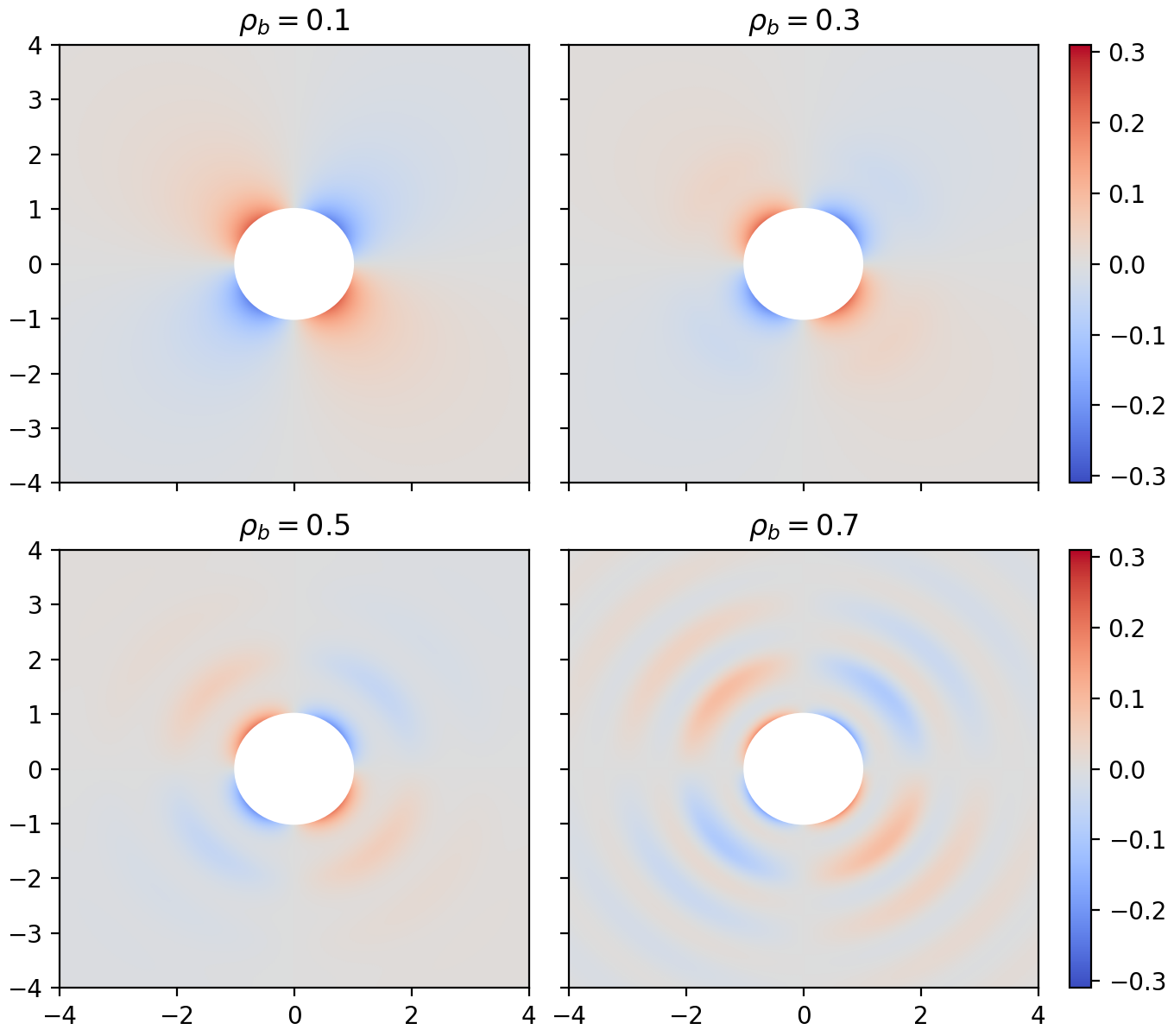
Figure 2: Superadiabatic-DDFT $g_{\text{sup}}$. For hard-disks in two-dimensions we show the superadiabatic contribution to the pair correlation function, $g_{\text{sup}}$, in units of $\dot{\gamma}d^{2}/2D_{0}$. Since we consider only low shear-rates $g_{\text{sup}}$ exhibits quadipolar symmetry, see equation (15). Increasing the bulk density leads to packing oscillations.

In Fig. 2, we show scatter plots of the rescaled superadiabatic contribution to the distorted pair correlation function, namely

$$\frac{g_{\text{sup}}(x,y)}{\dot{\gamma}d^{2}/2D_{0}}=-\frac{xy}{r^{2}}f(r),$$ (21)

where $r\!=\!\sqrt{x^{2}+y^{2}}$ and $f(r)$ is obtained from the numerical integration of equation (II.2). Results are shown for four different values of the bulk density, $\rho_{b}$, one per panel, and are valid at low shear-rates. At the lowest considered bulk density, $\rho_{b}\!=\!0.1$, the radial function $f(r)$ obtained numerically is very close to its low-density limit value, $f(r)\!=\!1/2r^{2}$, and no packing oscillations are visible in the resulting scaled $g_{\text{sup}}$. In this panel we observe an accumulation of particles at contact, $r\!=\!d$, in the ‘compressional’ quadrants, defined as the region where $\text{sign}(y)\!=\!-\text{sign}(x)$, and an opposite depletion effect in the ‘extensional’ quadrants, where $\text{sign}(y)\!=\!\text{sign}(x)$. As the value of the bulk density is increased packing oscillations develop at larger values of $r$. These oscillations in $g_{\text{sup}}$ take both positive and negative values and are a nontrivial prediction of the radial balance equation (II.2). The packing structure of the full pair correlation function, $g(\mathrm{\mathbf{r}})\!=\!g_{\text{eq}}(r)+g_{\text{sup}}(\mathrm{\mathbf{r}})$, will thus differ from that observed in bulk as a consequence of the applied shear. However, our numerical solutions reveal that the contact value of the radial function remains unaffected by changes in $\rho_{b}$ and is given by

$$f(r\!=\!d)=1/(2d^{2}),\quad\forall\rho_{b},$$ (22)

in each of the panels shown in Fig. 2.

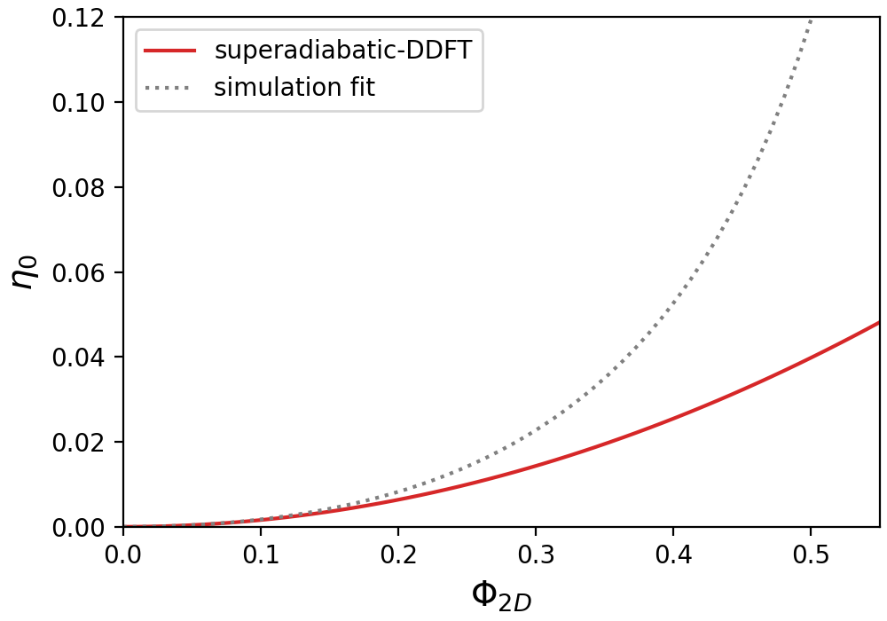
Figure 3: Low-shear viscosity. A comparison of $\eta_{0}$ from superadiabatic-DDFT, see equation (23), with a fit to simulation data, taken from reference [51]. The low-shear viscosity from simulation diverges as the system approaches random close packing, whereas the superadiabatic-DDFT retains the low density limiting form for all values of the area fraction.

Knowledge of the nonequilibrium pair correlation function also enables calculation of the interaction contribution to the low-shear viscosity, $\eta_{0}$, via equation (18). Results obtained by solving the radial balance equation (II.2) and evaluating the integral (18) for each chosen value of the bulk density are shown in Fig. 3 and compared with a fit to Brownian dynamics simulation data taken from reference [51]. While both curves overlap for low values of $\rho_{b}$, the theoretical superadiabatic-DDFT curve strongly underestimates $\eta_{0}$ relative to the simulation at higher densities. We note that the simulation curve diverges as the system approaches random close packing, located at $\Phi_{\text{2D}}\!\approx\!0.82$ for monodisperse hard-disks.

Due to the density independence of the contact value (22), the above described route to obtaining the interaction contribution to the low-shear viscosity recovers its low-density form, namely

$$\eta_{0}=\frac{k_{B}Td^{2}}{D_{0}}\frac{\Phi_{\text{2D}}^{2}}{2\pi},\quad\forall\rho_{b}.$$ (23)

Accounting for the influence of shear-flow on the bulk three-body density would give corrections to higher-order in area fraction in equation (23). However this mechanism is neglected per construction within the current approximation.

III Russel-Gast-type theory

In the preceding section we analysed the properties of superadiabatic-DDFT for bulk systems subject to homogeneous shear. All predictions of the theory for the pair distribution function and viscosity arise from the adiabatic closure employed to arrive at equation (2). In this section we show that there exists an alternative way to implement the adiabatic closure and that this results in a new approximate equation of motion for the inhomogeneous two-body density, different from equation (2). In the bulk limit the new approximation reduces to an equation of motion for the pair distribution function first introduced in 1986 by Russel and Gast [10] and which constituted one of the earliest theoretical approaches to the microstructure and rheology of colloidal suspensions at finite volume fraction. It thus seems appropriate to call our adiabatic closure of the equation of motion for the inhomogeneous two-body density a ‘Russel-Gast-type’ approximation.

III.1 Alternative adiabatic closure

Integrating the many-particle Smoluchowski equation over $N\!-\!2$ particle coordinates yields the following, formally exact equation of motion for the two-body density [44, 41]

$$\frac{1}{D_{0}}\, \frac{\partial\rho^{(2)}(\mathrm{\mathbf{r}}_{1},\mathrm{\mathbf{r}}_{2},t)}{\partial t}=\sum_{i=1,2}\nabla_{\mathrm{\mathbf{r}}_{i}}\cdot\Bigg{(}\!\nabla_{\mathrm{\mathbf{r}}_{i}}\rho^{(2)}(\mathrm{\mathbf{r}}_{1},\mathrm{\mathbf{r}}_{2},t)$$

$$\quad+\rho^{(2)}(\mathrm{\mathbf{r}}_{1},\mathrm{\mathbf{r}}_{2},t)\nabla_{\mathrm{\mathbf{r}}_{i}}\beta\big{(}V_{\text{ext}}(\mathrm{\mathbf{r}}_{i})+\phi(r_{12})\big{)}$$

$$\quad+\!\int d\mathrm{\mathbf{r}}_{3}\,\rho^{(3)}(\mathrm{\mathbf{r}}_{1},\mathrm{\mathbf{r}}_{2},\mathrm{\mathbf{r}}_{3},t)\nabla_{\mathrm{\mathbf{r}}_{i}}\beta\phi(r_{i3})\!\Bigg{)}.$$ (24)

This equation can also be rewritten in the following alternative form

$$\frac{1}{D_{0}}\, \frac{\partial\rho^{(2)}(\mathrm{\mathbf{r}}_{1},\mathrm{\mathbf{r}}_{2},t)}{\partial t}=$$

$$\sum_{i=1,2}\nabla_{\mathrm{\mathbf{r}}_{i}}\cdot\Bigg{(}\!\rho^{(2)}(\mathrm{\mathbf{r}}_{1},\mathrm{\mathbf{r}}_{2},t)\bigg{(}\!\nabla_{\mathrm{\mathbf{r}}_{i}}\ln\left(\rho^{(2)}(\mathrm{\mathbf{r}}_{1},\mathrm{\mathbf{r}}_{2},t)\right)$$

$$\quad+\nabla_{\mathrm{\mathbf{r}}_{i}}\beta\big{(}V_{\text{ext}}(\mathrm{\mathbf{r}}_{i})+\phi(r_{12})\big{)}$$

$$\quad+\!\int d\mathrm{\mathbf{r}}_{3}\,\frac{\rho^{(3)}(\mathrm{\mathbf{r}}_{1},\mathrm{\mathbf{r}}_{2},\mathrm{\mathbf{r}}_{3},t)}{\rho^{(2)}(\mathrm{\mathbf{r}}_{1},\mathrm{\mathbf{r}}_{2},t)}\nabla_{\mathrm{\mathbf{r}}_{i}}\beta\phi(r_{i3})\!\bigg{)}\!\Bigg{)},$$ (25)

which remains fully equivalent to equation (III.1), since there is no approximation involved at this stage.

Using the standard form (III.1) of the exact equation of motion and applying the adiabatic approximation solely on the three-body density, i.e. $\rho^{(3)}\!\rightarrow\!\rho^{(3)}_{\text{ad}}$, yields

$$\frac{1}{D_{0}}\, \frac{\partial\rho^{(2)}(\mathrm{\mathbf{r}}_{1},\mathrm{\mathbf{r}}_{2},t)}{\partial t}=\sum_{i=1,2}\nabla_{\mathrm{\mathbf{r}}_{i}}\cdot\Bigg{(}\!\nabla_{\mathrm{\mathbf{r}}_{i}}\rho^{(2)}(\mathrm{\mathbf{r}}_{1},\mathrm{\mathbf{r}}_{2},t)$$

$$\quad+\rho^{(2)}(\mathrm{\mathbf{r}}_{1},\mathrm{\mathbf{r}}_{2},t)\nabla_{\mathrm{\mathbf{r}}_{i}}\beta\big{(}V_{\text{ext}}(\mathrm{\mathbf{r}}_{i})+\phi(r_{12})\big{)}$$

$$\quad+\!\int d\mathrm{\mathbf{r}}_{3}\,\rho^{(3)}_{\text{ad}}(\mathrm{\mathbf{r}}_{1},\mathrm{\mathbf{r}}_{2},\mathrm{\mathbf{r}}_{3},t)\nabla_{\mathrm{\mathbf{r}}_{i}}\beta\phi(r_{i3})\!\Bigg{)},$$ (26)

where the adiabatic three-body density is defined as

$$\rho^{(3)}_{\text{ad}}(\mathrm{\mathbf{r}}_{1},\mathrm{\mathbf{r}}_{2},\mathrm{\mathbf{r}}_{3},t)\equiv\rho^{(3)}_{\text{eq}}(\textbf{r}_{1},\textbf{r}_{2},\textbf{r}_{3};[\rho(\textbf{r},t)]),$$ (27)

in analogy to equation (4). Substitution of the second-order Yvon-Born-Green (YBG2) equation [46, 41],

$$\int d\mathrm{\mathbf{r}}_{3}\, \rho_{\text{ad}}^{(3)}(\mathrm{\mathbf{r}}_{1},\mathrm{\mathbf{r}}_{2},\mathrm{\mathbf{r}}_{3},t)\nabla_{\mathrm{\mathbf{r}}_{i}}\beta\phi(r_{i3})=-\nabla_{\mathrm{\mathbf{r}}_{i}}\rho_{\text{ad}}^{(2)}(\mathrm{\mathbf{r}}_{1},\mathrm{\mathbf{r}}_{2},t)$$

$$-\rho_{\text{ad}}^{(2)}(\mathrm{\mathbf{r}}_{1},\mathrm{\mathbf{r}}_{2},t)\nabla_{\mathrm{\mathbf{r}}_{i}}\beta\big{(}V_{\text{ad}}(\mathrm{\mathbf{r}}_{i},t)+\phi(r_{12})\big{)},$$ (28)

into (III.1) yields the second equation of superadiabatic-DDFT, namely equation (2). This is the procedure followed in reference [41].

An alternative method to implement the adiabatic closure, is to start with the (reformulated) exact equation of motion (III.1) and to apply the approximation to the integral term,

$$\frac{1}{D_{0}}\, \frac{\partial\rho^{(2)}(\mathrm{\mathbf{r}}_{1},\mathrm{\mathbf{r}}_{2},t)}{\partial t}=$$

$$\sum_{i=1,2}\nabla_{\mathrm{\mathbf{r}}_{i}}\cdot\Bigg{(}\!\rho^{(2)}(\mathrm{\mathbf{r}}_{1},\mathrm{\mathbf{r}}_{2},t)\bigg{(}\!\nabla_{\mathrm{\mathbf{r}}_{i}}\ln\left(\rho^{(2)}(\mathrm{\mathbf{r}}_{1},\mathrm{\mathbf{r}}_{2},t)\right)$$

$$\quad+\nabla_{\mathrm{\mathbf{r}}_{i}}\beta\big{(}V_{\text{ext}}(\mathrm{\mathbf{r}}_{i})+\phi(r_{12})\big{)}$$

$$\quad+\!\int d\mathrm{\mathbf{r}}_{3}\,\frac{\rho^{(3)}_{\text{ad}}(\mathrm{\mathbf{r}}_{1},\mathrm{\mathbf{r}}_{2},\mathrm{\mathbf{r}}_{3},t)}{\rho^{(2)}_{\text{ad}}(\mathrm{\mathbf{r}}_{1},\mathrm{\mathbf{r}}_{2},t)}\nabla_{\mathrm{\mathbf{r}}_{i}}\beta\phi(r_{i3})\!\bigg{)}\!\Bigg{)}.$$ (29)

We note that equation (III.1) is no longer equivalent to the previous equation (III.1). The essential difference between these two options is that in equation (III.1) we approximate the joint probability density, whereas in equation (III.1) we approximate the conditional probability density. Substitution of the rewritten YBG2 equation,

$$\int d\mathrm{\mathbf{r}}_{3}\,\frac{\rho^{(3)}_{\text{ad}}(\mathrm{\mathbf{r}}_{1},\mathrm{\mathbf{r}}_{2},\mathrm{\mathbf{r}}_{3},t)}{\rho^{(2)}_{\text{ad}}(\mathrm{\mathbf{r}}_{1},\mathrm{\mathbf{r}}_{2},t)}\nabla_{\mathrm{\mathbf{r}}_{i}}\beta\phi(r_{i3})=$$ (30)

$$-\nabla_{\mathrm{\mathbf{r}}_{i}}\ln\left(\rho_{\text{ad}}^{(2)}(\mathrm{\mathbf{r}}_{1},\mathrm{\mathbf{r}}_{2},t)\right)-\nabla_{\mathrm{\mathbf{r}}_{i}}\beta\big{(}V_{\text{ad}}(\mathrm{\mathbf{r}}_{i},t)+\phi(r_{12})\big{)},$$

into expression (III.1), then yields the following alternative equation of motion for the two-body density

$$\frac{1}{D_{0}}\,\frac{\partial\rho^{(2)}(\mathrm{\mathbf{r}}_{1},\mathrm{\mathbf{r}}_{2},t)}{\partial t}=$$ (31)

$$\sum_{i=1,2}\nabla_{\mathrm{\mathbf{r}}_{i}}\cdot\Bigg{(}\!\rho^{(2)}(\mathrm{\mathbf{r}}_{1},\mathrm{\mathbf{r}}_{2},t)\bigg{(}\!\nabla_{\mathrm{\mathbf{r}}_{i}}\ln\left(\rho^{(2)}(\mathrm{\mathbf{r}}_{1},\mathrm{\mathbf{r}}_{2},t)\right)$$

$$\!+\nabla_{\mathrm{\mathbf{r}}_{i}}\beta\big{(}V_{\text{ext}}(\mathrm{\mathbf{r}}_{i})\!-\!V_{\text{ad}}(\mathrm{\mathbf{r}}_{i},t)\big{)}-\nabla_{\mathrm{\mathbf{r}}_{i}}\ln\left(\rho_{\text{ad}}^{(2)}(\mathrm{\mathbf{r}}_{1},\mathrm{\mathbf{r}}_{2},t)\right)\!\!\bigg{)}\!\Bigg{)}.$$

We refer to this approximation strategy as ‘Russel-Gast-like’, since equation (31) reduces to the Russel-Gast equation (see reference [10]) for the pair distribution function in the bulk limit, as we will demonstrate in the following subsection.

III.2 Low shear-rate solutions for the pair distribution function in bulk

Following the same scheme as in subsection II.2, the bulk limit of equation (31) is given by

$$\frac{\partial g(\mathrm{\mathbf{r}},t)}{\partial t}=-2D_{0}\nabla\cdot\Big{(}-\nabla g_{\text{sup}}(\mathrm{\mathbf{r}},t)+\frac{g_{\text{sup}}(\mathrm{\mathbf{r}},t)}{g_{\text{eq}}(r)}\nabla g_{\text{eq}}(r)\Big{)}\\ -\nabla\cdot\Big{(}g(\mathrm{\mathbf{r}},t)\,\mathrm{\mathbf{v}}(\mathrm{\mathbf{r}},t)\Big{)}.$$ (32)

This provides an alternative to equation (10). (As a side-note we mention that the second term on the right hand-side of equation (32) can be rewritten using the following rearrangement

$$\frac{g_{\text{sup}}(\mathrm{\mathbf{r}},t)}{g_{\text{eq}}(r)}\nabla g_{\text{eq}}(r) =-g_{\text{sup}}(\mathrm{\mathbf{r}},t)\nabla\Big{(}\!-\ln\big{(}g_{\text{eq}}(r)\big{)}\!\Big{)}$$

$$=-g_{\text{sup}}(\mathrm{\mathbf{r}},t)\nabla\Big{(}\beta\phi_{\text{mf}}(r)\Big{)},$$

where we have introduced the ‘potential of mean force’, $\phi_{\text{mf}}(r)$, defined by $g_{\text{eq}}(r)\!\equiv\!e^{-\beta\phi_{\text{mf}}(r)}$.) In the low density limit, $g_{\text{eq}}(r)\!\rightarrow\!e^{-\beta\phi(r)}$, which yields

$$\frac{g_{\text{sup}}(\mathrm{\mathbf{r}},t)}{g_{\text{eq}}(r)}\nabla g_{\text{eq}}(r)\rightarrow-g_{\text{sup}}(\mathrm{\mathbf{r}},t)\nabla\beta\phi(r),$$ (33)

such that equations (32) and (10) then become equivalent (which is not the case in general).

In the steady-state at finite densities, equation (32) reduces to the condition

$$2D_{0}\nabla\cdot\Big{(}\nabla g_{\text{sup}}(\mathrm{\mathbf{r}},t)-\frac{g_{\text{sup}}(\mathrm{\mathbf{r}},t)}{g_{\text{eq}}(r)}\nabla g_{\text{eq}}(r)\Big{)}\\ -\nabla\cdot\Big{(}g(\mathrm{\mathbf{r}},t)\,\mathrm{\mathbf{v}}(\mathrm{\mathbf{r}},t)\Big{)}=0.$$ (34)

Using the definition (12) and again assuming that $g_{\text{sup}}$ is linear in the flow-rate yields the following expression to leading order

$$2D_{0}\nabla\cdot\Big{(}\nabla g_{\text{sup}}(\mathrm{\mathbf{r}},t)-\frac{g_{\text{sup}}(\mathrm{\mathbf{r}},t)}{g_{\text{eq}}(r)}\nabla g_{\text{eq}}(r)\Big{)}\\ -\nabla\cdot\Big{(}g_{\text{eq}}(r)\,\mathrm{\mathbf{v}}(\mathrm{\mathbf{r}})\Big{)}=0.$$ (35)

Since equations (14) and (35) are non-equivalent the solution of equation (35) now requires a different ansatz than used previously. The appropriate choice in the present case is given by

$$g_{\text{sup}}(\mathrm{\mathbf{r}})=-\frac{1}{2D_{0}}\left(\frac{\mathrm{\mathbf{r}}\cdot\mathbb{E}\cdot\mathrm{\mathbf{r}}}{r^{2}}\right)g_{\text{eq}}(r)f^{\star}(r),$$ (36)

where the $\star$ notation makes it explicit that the (still unknown) radial function, $f^{\star}(r)$, is different from the function, $f(r)$, previously encountered. Substitution of ansatz (36) into the linearized steady-state equation (35) then yields the alternative radial balance equations

$$\frac{dg_{\text{eq}}(r)}{dr} \,\overset{\text{2D}}{=}\,-\frac{1}{r^{2}}\frac{d}{dr}\Big{(}r\frac{df^{\star}(r)}{dr}g_{\text{eq}}(r)\Big{)}\;\,+\frac{4}{r^{3}}f^{\star}(r)g_{\text{eq}}(r),$$

$$\frac{dg_{\text{eq}}(r)}{dr} \,\overset{\text{3D}}{=}\,-\frac{1}{r^{3}}\frac{d}{dr}\Big{(}r^{2}\frac{df^{\star}(r)}{dr}g_{\text{eq}}(r)\Big{)}+\frac{6}{r^{3}}f^{\star}(r)g_{\text{eq}}(r),$$ (37)

to determine $f^{\star}(r)$, for the cases of two- and three-dimensions. We refer the reader to appendix D for additional details regarding the derivation of equations (III.2) and the boundary conditions required to solve them.

III.3 Low-shear viscosity

Within the alternative adiabatic closure the low-shear viscosity is given by

$$\eta_{0}=\frac{k_{B}T}{4D_{0}}\,\rho_{b}^{2}\int\!d\mathrm{\mathbf{r}}\frac{x^{2}y^{2}}{r^{3}}\left(\frac{d}{dr}e^{-\beta\phi(r)}\right)y_{\text{eq}}(r)f^{\star}(r),$$ (38)

where we have introduced the so-called ‘cavity distribution function’,

$$y_{\text{eq}}(r)=g_{\text{eq}}(r)\,e^{\beta\phi(r)},$$ (39)

familiar from liquid-state theory [46]. We emphasize that $f^{\star}(r)$ appearing in equation (38) is given by solution of the radial balance equations (III.2) and is distinct from the function $f(r)$ obtained from solution of equations (II.2). In two- and three-dimensions equation (38) becomes

$$\eta_{0} \,\overset{\text{2D}}{=}\;\frac{k_{B}T}{\pi D_{0}}\,\Phi_{\text{2D}}^{2}\int_{0}^{\infty}\!dr\,r^{2}\left(\frac{d}{dr}e^{-\beta\phi(r)}\right)y_{\text{eq}}(r)f^{\star}(r),$$

$$\eta_{0} \,\overset{\text{3D}}{=}\;\frac{k_{B}T}{\pi D_{0}}\,\frac{12}{5}\,\Phi_{\text{3D}}^{2}\int_{0}^{\infty}\!dr\,r^{3}\left(\frac{d}{dr}e^{-\beta\phi(r)}\right)y_{\text{eq}}(r)f^{\star}(r),$$ (40)

respectively. For the special case of low density hard-spheres in three-dimensions, the analytic solution of equation (III.2) is the same as that given by equation (II.2), namely

$$f^{\star}(r)\!=\!f(r)\!=\!1/(3r^{3}),$$ (41)

such that the Russel-Gast-type closure reproduces the exact low density expansion of the low-shear viscosity of hard-spheres, given by equation (20).

III.4 Numerical results

We now investigate some numerical predictions of the alternative closure, where we again consider the hard-disk system in two-dimensions and use the Percus-Yevick closure to obtain $g_{\text{eq}}$ for input to the radial balance equation (III.2).

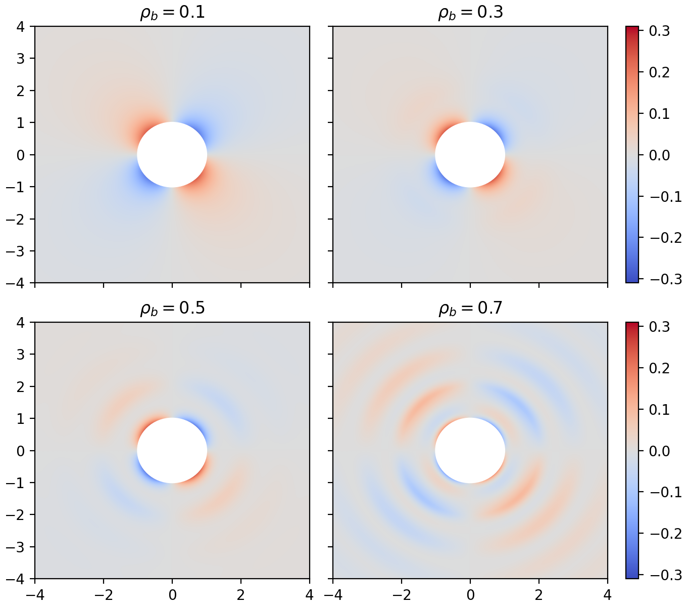
Figure 4: Russel-Gast-type closure for $g_{\text{sup}}$. Analogous plot to Fig. 2, but this time employing the alternative closure. For hard-disks we show the superadiabatic contribution to the pair correlation function, $g_{\text{sup}}$, in units of $\dot{\gamma}d^{2}/2D_{0}$, see equation (36). Since the results are qualitatively similar to those in Fig. 2 and thus difficult to compare, we refer the reader to Fig. 5 for a more detailed analysis.

In Fig. 4 we show scatter plots of the quantity

$$\frac{g_{\text{sup}}(x,y)}{\dot{\gamma}d^{2}/2D_{0}}=-\frac{xy}{r^{2}}f^{\star}(r)g_{\text{eq}}(r),$$ (42)

for four different values of the input bulk density. Note that the radial function $f^{\star}(r)$ is obtained from numerical integration of equation (III.2) and that $r\!=\!\sqrt{x^{2}+y^{2}}$. The predictions of the Russel-Gast-type closure are generally very similar to those obtained from the superadiabatic-DDFT approach of the previous section, although deviations become apparent on closer inspection.

The results for $g_{\text{sup}}$ at the lowest bulk density considered, $\rho_{b}\!=\!0.1$, are very close to the known low-density limit, for which $f^{\star}(r)\!=\!1/2r^{2}$, with accumulation and depletion at contact within the compressional and extensional quadrants, respectively. As the bulk density is increased we observe the emergence of packing oscillations. We recall that superadiatic-DDFT predicted that the radial function $f$ appearing in equation (23) has a contact value which remains independent of the bulk density. The analogous quantity within the present approximation is the product $f^{\star}(r)\,g_{\text{eq}}(r)$ appearing on the right hand-side of equation (42). We find that the contact value of this product does exhibit a nontrivial dependence on $\rho_{b}$ and, as we will see, this causes the low-shear viscosity generated by equation (III.3) to deviate from that predicted by superadiabatic-DDFT.

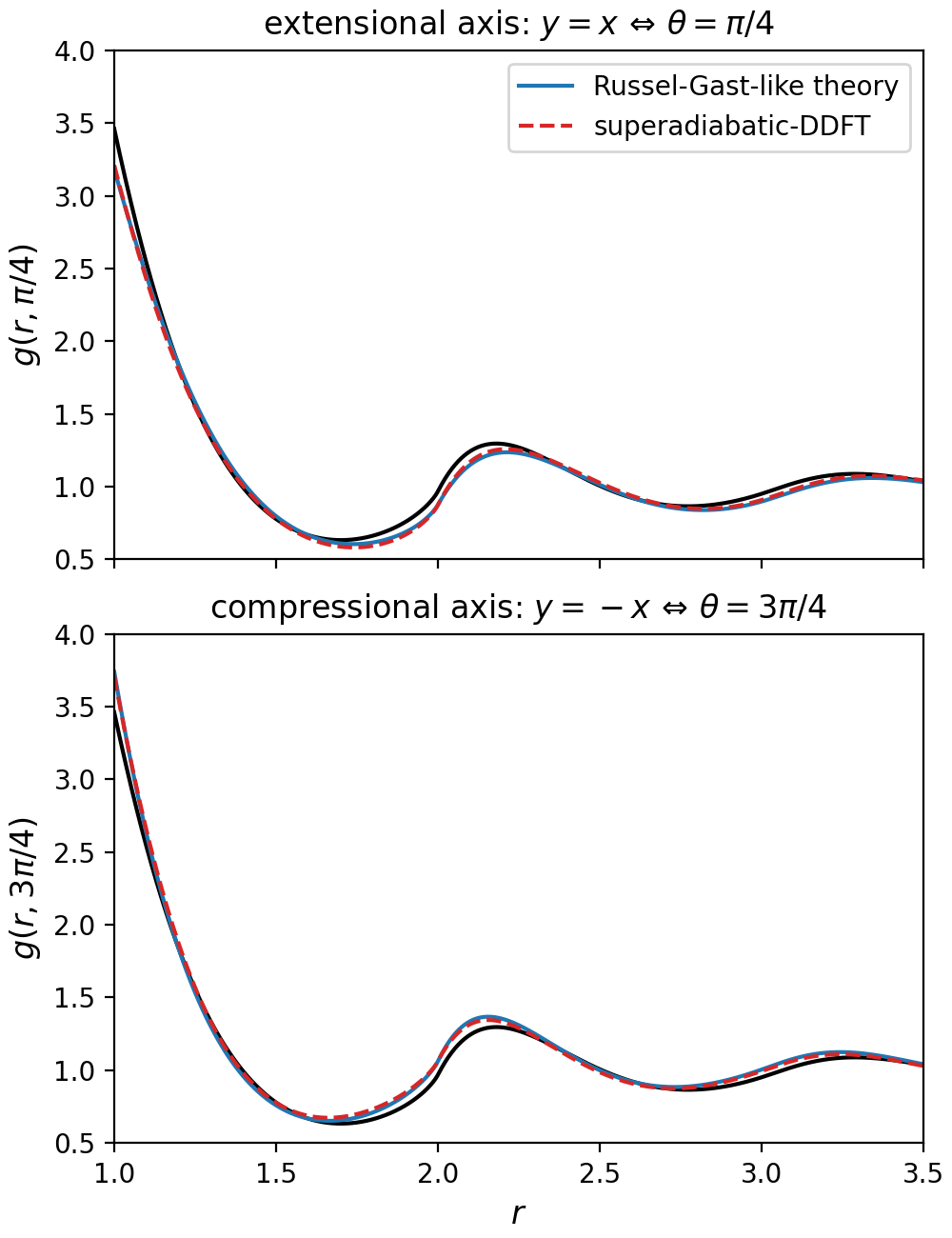
Figure 5: Pair distribution function. We show the full nonequilibrium pair distribution function of hard-disks along the extensional axis, $y\!=\!x$, and the compressional axis, $y\!=\!-x$. Results are given from both the superadiabatic-DDFT and the Russel-Gast-type approximations, for $\rho_{b}\!=\!0.7$. The additional black curve indicates the equilibrium radial distribution function for comparison. The dimensionless shear-rate is chosen to be $\dot{\gamma}d^{2}/2D_{0}\!=\!1$.

In Fig. 5 we show the pair distribution function on both the extensional axis, along which the particles get pulled apart by the shear, and on the compressional axis, along which the particles get pressed together. On the extensional axis both approximation schemes predict a reduction in the height of all maxima, including the first peak at particle contact. The reduction in amplitude of the peaks is slightly more pronounced within the Russel-Gast-type approximation. In both cases the radial position of the second and higher-order peaks shifts to larger values of $r$, consistent with the fact that particles are being pulled away from each other by the shear flow. In contrast, on the compressional axis the height of all maxima increase and the radial locations of the second and higher-order peaks are shifted to smaller values of $r$, since the particles are being pushed closer together by the shear flow. The two theories again make similar predictions, although the Russel-Gast-type approximation yields a slightly larger increase in peak height than the superadiabatic-DDFT. The general similarity of the predictions from the two approximation schemes for the nonequilibrium microstructure is reassuring, as it appears that the results are robust with respect to the details of how the adiabatic approximation is implemented.

From the nonequilibrium pair correlation function we can calculate the zero-shear viscosity using equation (III.3), for which results are shown in Fig. 6. We find that the Russel-Gast-type approximation scheme generates a low-shear viscosity curve with values slightly larger than that predicted by the superadiabatic-DDFT. We can attribute this effect to the difference in the contact value of the pair distribution function between the two approximations, see Fig. 5. Within the Russel-Gast-type approach the difference between the contact value on the extensional axis and the contact value on the compressional axis is larger than for superadiabatic-DDFT. This larger extensional/compressional asymmetry has the consequence that for any given area fraction $\eta_{0}$ from the Russel-Gast-type approach is larger than for the superadiabatic-DDFT. Although the Russel-Gast-type closure produces values of the low-shear viscosity closer to the simulation results, it has the undesirable feature of changing curvature as the area fraction increases beyond about $0.45$. This questions the physicality of the alternative approximation and its rescaling potential for higher densities [12].

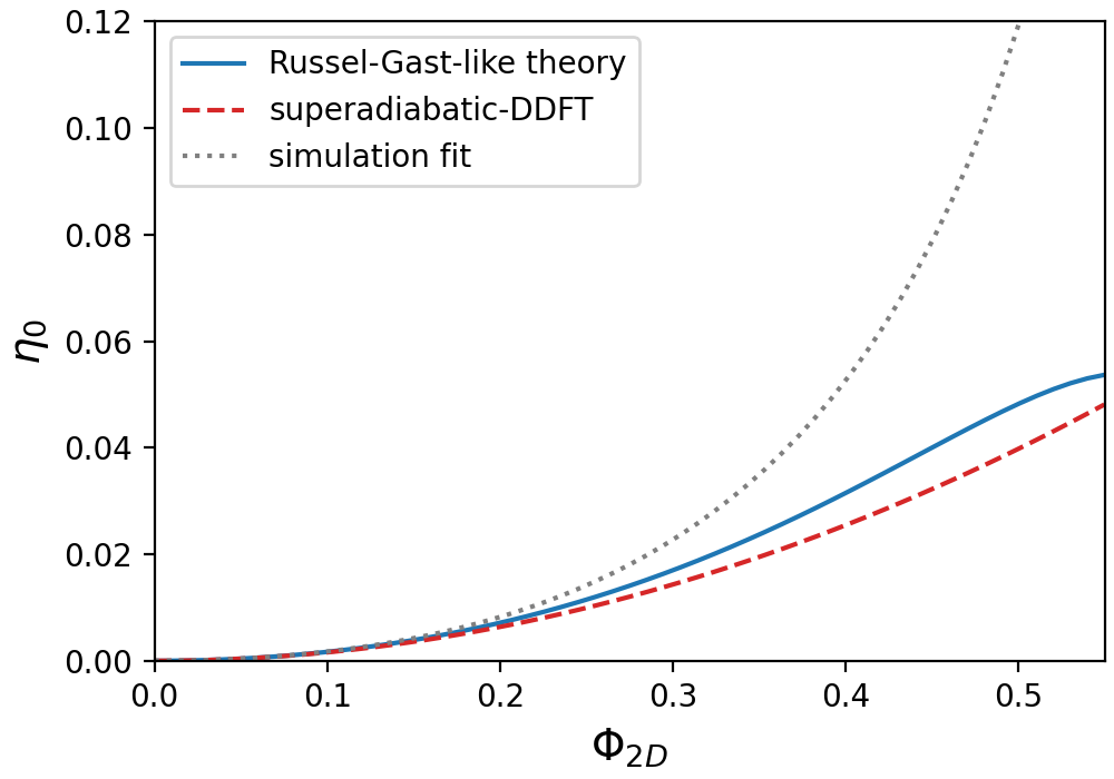
Figure 6: Low-shear viscosity. Analogous plot to Fig. 3, but now including the prediction of the Russel-Gast-type approximation. This additional result predicts slightly larger values of $\eta_{0}$ than the superadiabatic-DDFT, but exhibits an unphysical curvature as the area fraction is increased.

IV Discussion

In this paper we have investigated the predictions of superadiabatic-DDFT for the nonequilibrium pair correlation function and low-shear viscosity of bulk systems subject to the homogeneous shear flow defined by equation (9). This provides a conceptual link between density functional-based approaches, which are focused on the inhomogeneous one-body density [43, 44, 52], and microscopic theories of homogeneous bulk rheology, of the type pioneered by Brady, Russel, Wagner and others [18, 2, 3]. A clear connection between these two substantial bodies of literature, which have coexisted for decades with little to no interaction, is established by our Russel-Gast-type closure of the equation of motion for the two-body density. As detailed in section III, this new scheme generates a fully inhomogeneous DDFT, which reduces to the known Russel-Gast theory for bulk systems subject to homogeneous shear [10].

The application of shear distorts the bulk pair distribution function and, for systems interacting via a pairwise additive potential, enables the interaction part of the stress tensor to be calculated. For the low shear-rates considered here the only relevant transport coefficient is the viscosity, since the lowest-order shear-induced changes to the diagonal stress tensor elements are quadratic in $\dot{\gamma}$. For larger shear-rates we would need to consider the extension of our solution ansatz (15) or (36), respectively, to higher-order in $\dot{\gamma}$, which would then generate nonvanishing normal stress differences and shear-induced modifications to the system pressure [6, 29].

Focusing on the low shear-rate regime enabled a largely analytic investigation of the nonequilibrium pair distribution function, with only the solution of the radial balance equation and evaluation of the low-shear viscosity demanding (relatively simple) numerical integration. At larger values of the shear-rate more sophisticated techniques must be employed, since boundary-layer formation prevents the application of straightforward perturbation theory [53, 6, 54, 55, 56]. An interesting extension of our study to obtain results for higher shear-rates could be to employ either multipole methods [57], specialized numerical schemes [6, 58] or intermediate asymptotics [19, 56]. Although the theories presented here are valid for an arbitrary pair interaction potential in two- or three-dimensions, we chose to perform numerical calculations for the special case of hard-disks, as this presents the simplest continuum model for the study of shear, while still retaining much of the essential phenomenology of three-dimensional systems. In references [19, 56] it is shown how the pair distribution function under shear can be calculated analytically for more general interaction potentials.

The two routes presented in this work are built on two variations of the same approximation. The numerical output of those theories is broadly similar but, as clearly pictured by the final viscosity plot, Fig. 6, are different in more demanding situations at higher bulk density. One can thus ask which scheme is more likely to succeed in further investigations. The unphysical shape of the viscosity curve obtained with the Russel-Gast-like closure suggests that this variation of the approximation may be less robust than that of superadiabatic-DDFT and could prove more difficult to improve and refine.

A natural first step towards better predictions for the viscosity at higher bulk densities would be to apply Brady’s semi-empirical rescaling method [12]. For the present Brownian dynamics, without hydrodynamic interactions, this consists of multiplying the low density limiting solution for the interaction contribution to $\eta_{0}$ (given by equation (23) for hard-disks) by the contact value of the equilibrium radial distribution function. The resulting low-shear viscosity has been shown to agree well with simulation data for hard-spheres [16] and we find that this is also the case for hard-disks. Since the superadiabatic-DDFT predicts that the low-density limiting result (23) holds for all values of $\rho_{b}$, a rescaled version of superadiatic-DDFT would exactly reproduce Brady’s theory for $\eta_{0}$. In contrast, a rescaled Russel-Gast-type theory would continue to exhibit an unphysical curvature, as the contact value of $g_{\text{eq}}$ is a monotonically increasing function of bulk density. Investigating how such a rescaling factor could emerge from a systematic, first-principles extension of the superadiabatic-DDFT closure scheme will be an interesting topic for future study.

A further challenge to the superadiabatic-DDFT is presented when the shear-rate becomes large. In this case, it is known from both simulation [37] and experiment [59] that the nonequilibrium bulk three-body distribution function deviates significantly from its equilibrium form. Although further investigation is required, we anticipate that some of the shear-induced changes to the microstructure will not be captured by direct application of the superadiabatic-DDFT to the bulk system, as we have done in the present work. A more sophisticated implementation scheme, which would probably extract much improved predictions from the existing superadiabatic-DDFT approach, would be to exploit this fully inhomogeneous theory in a test-particle calculation. Fixing a particle at the coordinate origin (i.e. setting $V_{\text{ext}}(\mathrm{\mathbf{r}})\!=\!\phi(r)$) would induce a spatially varying, anisotropic one-body density, $\rho(\mathrm{\mathbf{r}})$, as particles around the test-particle accumulate in the compressional quadrants and are depleted from the extensional quadrants [51]. This inhomogeneous one-body density can then be related to the bulk pair distribution function according to $g(\mathrm{\mathbf{r}})\!=\!\rho(\mathrm{\mathbf{r}})/\rho_{b}$. Implementation of the superadiabatic-DDFT would involve dealing with the inhomogeneous two-body density in the presence of a test-particle and would thus capture, to some extent, the shear-induced distortion of the bulk three-body correlations. Investigations in this direction are underway.

Finally, we mention the issue of hydrodynamic interactions. Although the majority of standard DDFT studies do not consider solvent hydrodynamics, this aspect has been incorporated into the formalism [60, 61, 62, 63, 64]. It would thus be interesting to investigate whether a similar extension would be feasable for superadiabatic-DDFT. Many of the existing theories of homogeneous bulk rheology mentioned in the introduction, including the bulk Russel-Gast theory, were formulated to include hydrodynamic interactions to some level of approximation. These works, all of which are focused on the two-body correlations, could well provide a source of inspiration for future developments.

Appendix A Rheological quantities

In a system undergoing translationally invariant, homogeneous flow, the velocity field can be conveniently expressed in the following form

$$\mathrm{\mathbf{v}}(\mathrm{\mathbf{r}})=\boldsymbol{\kappa}\cdot\mathrm{\mathbf{r}},$$ (43)

where $\boldsymbol{\kappa}$ is the spatially constant velocity gradient tensor. As an example, choosing flow in the $x$-direction, with shear-gradient in the $y$-direction enables $\boldsymbol{\kappa}$ to be represented in matrix form as

$$\boldsymbol{\kappa}=\begin{pmatrix}0&\dot{\gamma}&0\\ 0&0&0\\ 0&0&0\end{pmatrix},$$ (44)

for a three-dimensional system with shear-rate $\dot{\gamma}$.

The right hand-side of (43) can be decomposed into a sum of two terms,

$$\mathrm{\mathbf{v}}(\mathrm{\mathbf{r}})={\bf E}\cdot\mathrm{\mathbf{r}}+{\boldsymbol{\Omega}}\cdot\mathrm{\mathbf{r}},$$ (45)

where

$${\bf E}=\frac{1}{2}\left({\boldsymbol{\kappa}}+{\boldsymbol{\kappa}}^{\text{T}}\right),\quad{\boldsymbol{\Omega}}=\frac{1}{2}\left({\boldsymbol{\kappa}}-{\boldsymbol{\kappa}}^{\text{T}}\right),$$ (46)

are the (symmetric) rate-of-strain tensor and the (antisymmetric) rate-of-rotation tensor, respectively. The rate-of-strain tensor describes ‘pure straining motion’ leading to relative motion between any two particles, whereas the rate-of-rotation tensor yields pure rotational motion, which does not affect their relative separation [65]. For the aforementioned case of shear flow we obtain

$$\boldsymbol{{\bf E}}=\frac{1}{2}\begin{pmatrix}0&\dot{\gamma}&0\\ \dot{\gamma}&0&0\\ 0&0&0\end{pmatrix},\quad\boldsymbol{{\boldsymbol{\Omega}}}=\frac{1}{2}\begin{pmatrix}\;\;0&\dot{\gamma}&0\\ \!\!\!-\dot{\gamma}&0&0\\ \;\;0&0&0\end{pmatrix}.$$ (47)

The anisotropy of the nonequilibrium pair distribution function in a system subject to a slow translationally invariant flow is determined solely by its straining motion and does not involve its rotational component [18, 6]. This motivates our choice of ansatz for $g_{\text{sup}}$ in equations (15) and (36).

Appendix B The radial balance equation

Substitution of the ansatz (15) into the linearized steady-state equation (14) yields the radial balance equations (II.2). Since this procedure is not straightforward we outline here the main steps of the calculation. Although we are primarily interested in the case of homogeneous shear, we formulate the problem using the rate-of-flow tensor ${\bf E}$, which can also describe other flow types. This not only extends the generality of our results, but also presents the technical advantage that certain vector/tensor identities can be employed to make the calculation as clean as possible. Unless otherwise stated, all expressions given in this appendix are valid in arbitrary dimensionality.

We start by collecting a few useful identities. For a general, spatially varying, second-rank tensor ${\bf M}$ the following holds

$$\nabla\big{(}\left(\hat{\mathrm{\mathbf{r}}}\cdot{\bf M}\cdot\hat{\mathrm{\mathbf{r}}}\right)\,a(r)\big{)} =\frac{2}{r^{2}}(\mathrm{\mathbf{r}}\cdot{\bf M})\cdot(\mathds{1}-\hat{\mathrm{\mathbf{r}}}\hat{\mathrm{\mathbf{r}}})\,a(r)$$

$$+\frac{1}{r}\frac{da(r)}{dr}(\mathrm{\mathbf{r}}\cdot{\bf M})\cdot\hat{\mathrm{\mathbf{r}}}\hat{\mathrm{\mathbf{r}}},$$ (48)

where $\hat{\mathrm{\mathbf{r}}}\!=\!\mathrm{\mathbf{r}}/r$ is a unit vector, $\hat{\mathrm{\mathbf{r}}}\hat{\mathrm{\mathbf{r}}}$ is a dyadic product and where $a(r)$ is a scalar function of $r\!=\!|\mathrm{\mathbf{r}}|$. For an arbitrary, spatially dependent vector field, $\mathrm{\mathbf{u}}$, we have

$$\nabla\cdot\left(\textbf{u}\cdot\mathbb{M}\right)=\textbf{u}\cdot\left(\nabla\cdot\mathbb{M}\right)+\mathbb{M}:\nabla\textbf{u},$$ (49)

where the double dot notation in the second term indicates a full contraction, i.e. a scalar product followed by a trace operation. The divergence of the product $a(r){\bf M}$ is given by

$$\begin{split}\nabla\cdot\left(a(r)\mathbb{M}\right)&=\nabla a(r)\cdot\mathbb{M}+a(r)\,\nabla\cdot\mathbb{M}\\ &=\left(\frac{da(r)}{dr}\right)\hat{\textbf{r}}\cdot\mathbb{M}+a(r)\,\nabla\cdot\mathbb{M}.\end{split}$$ (50)

This identity generates the following special cases in two-dimensions

$$\nabla\cdot\big{(}\,a(r)\left(\mathds{1}-\hat{\textbf{r}}\hat{\textbf{r}}\right)\big{)}\overset{\text{2D}}{=}-\frac{a(r)}{r}\,\hat{\mathrm{\mathbf{r}}},$$ (51)

$$\nabla\cdot\big{(}\,a(r)\,\hat{\textbf{r}}\hat{\textbf{r}}\,\big{)}\overset{\text{2D}}{=}\frac{1}{r}\frac{d}{dr}\Big{(}ra(r)\Big{)}\hat{\mathrm{\mathbf{r}}},$$ (52)

and three-dimensions

$$\nabla\cdot\big{(}\,a(r)\left(\mathds{1}-\hat{\textbf{r}}\hat{\textbf{r}}\right)\big{)}\overset{\text{3D}}{=}-\frac{2a(r)}{r}\,\hat{\mathrm{\mathbf{r}}},$$ (53)

$$\nabla\cdot\big{(}\,a(r)\,\hat{\textbf{r}}\hat{\textbf{r}}\,\big{)}\overset{\text{3D}}{=}\frac{1}{r^{2}}\frac{d}{dr}\Big{(}r^{2}a(r)\Big{)}\hat{\mathrm{\mathbf{r}}},$$ (54)

respectively. In the special case that ${\bf M}$ is symmetric it can be shown that

$$\big{(}\nabla\left({\bf M}\cdot\hat{\mathrm{\mathbf{r}}}\right)\big{)}\cdot\hat{\mathrm{\mathbf{r}}}=0.$$ (55)

Finally, the divergence of the scalar product ${\bf M}\cdot\hat{\mathrm{\mathbf{r}}}$ is given by the aesthetically appealing identity

$$\nabla\cdot\left({\bf M}\cdot\hat{\mathrm{\mathbf{r}}}\right)=\frac{{\rm Tr}\left({\bf M}\right)}{r}-\frac{\hat{\mathrm{\mathbf{r}}}\cdot{\bf M}\cdot\hat{\mathrm{\mathbf{r}}}}{r}.$$ (56)

We will now employ these identities to calculate the pair distribution function at low flow-rate.

Substitution of the ansatz (15) into the linearized steady-state equation (14) yields

$$\nabla\cdot\Big{(}g_{\text{eq}}(r)\mathrm{\mathbf{v}}(\mathrm{\mathbf{r}})\Big{)}=-\nabla\cdot\Big{(}e^{-\beta\phi(r)}\,\nabla\big{(}\left(\hat{\mathrm{\mathbf{r}}}\cdot{\bf E}\cdot\hat{\mathrm{\mathbf{r}}}\right)f(r)\big{)}\Big{)},$$ (57)

in which the only unknown quantity is the function $f(r)$. Assuming incompressible flow, $\nabla\cdot\mathrm{\mathbf{v}}\!=\!0$, using identity (B) and rewriting the projected velocity as

$$\mathrm{\mathbf{v}}(\mathrm{\mathbf{r}})\cdot\hat{\mathrm{\mathbf{r}}}=r\left(\hat{\mathrm{\mathbf{r}}}\cdot{\bf E}\cdot\hat{\mathrm{\mathbf{r}}}\right),$$ (58)

enables us to re-express equation (57) as follows

$$r\frac{dg_{\text{eq}}(r)}{dr}\,\big{(}\hat{\mathrm{\mathbf{r}}}\cdot{\bf E}\cdot\hat{\mathrm{\mathbf{r}}}\big{)}=$$ (59)

$$-\nabla\cdot\bigg{(}\big{(}\hat{\mathrm{\mathbf{r}}}\cdot{\bf E}\big{)}\cdot\bigg{(}(\mathds{1}-\hat{\mathrm{\mathbf{r}}}\hat{\mathrm{\mathbf{r}}})\frac{2f(r)}{r}+\hat{\mathrm{\mathbf{r}}}\hat{\mathrm{\mathbf{r}}}\frac{df(r)}{dr}\bigg{)}e^{-\beta\phi(r)}\bigg{)}.$$

The advantage of this representation is the appearance of the dyadic tensors, $\hat{\mathrm{\mathbf{r}}}\hat{\mathrm{\mathbf{r}}}$ and $(\mathds{1}-\hat{\mathrm{\mathbf{r}}}\hat{\mathrm{\mathbf{r}}})$, which project either along or perpendicular to the relative position vector $\mathrm{\mathbf{r}}$.

On the right hand-side of (59) we have to calculate the divergence of the scalar product between the vector $\hat{\mathrm{\mathbf{r}}}\cdot{\bf E}$ and a second-rank tensor. We can thus exploit relation (49) to obtain

$$r\frac{dg_{\text{eq}}(r)}{dr}\,\big{(}\hat{\mathrm{\mathbf{r}}}\cdot{\bf E}\cdot\hat{\mathrm{\mathbf{r}}}\big{)} =$$

$$-\left(\hat{\mathrm{\mathbf{r}}}\cdot{\bf E}\right)\cdot\bigg{(}\nabla\cdot\bigg{(}\!\bigg{(}(\mathds{1}-\hat{\mathrm{\mathbf{r}}}\hat{\mathrm{\mathbf{r}}})\frac{2f(r)}{r}+\hat{\mathrm{\mathbf{r}}}\hat{\mathrm{\mathbf{r}}}\frac{df(r)}{dr}\bigg{)}e^{-\beta\phi(r)}\bigg{)}\!\bigg{)}$$

$$-\left(\!\bigg{(}(\mathds{1}-\hat{\mathrm{\mathbf{r}}}\hat{\mathrm{\mathbf{r}}})\frac{2f(r)}{r}+\hat{\mathrm{\mathbf{r}}}\hat{\mathrm{\mathbf{r}}}\frac{df(r)}{dr}\bigg{)}e^{-\beta\phi(r)}\right):\nabla\left({\bf E}\cdot\hat{\mathrm{\mathbf{r}}}\right).$$ (60)

We will consider separately the two terms appearing on the right hand-side of (B), which we henceforth refer to as $(i)$ and $(ii)$.

To simplify $(i)$ in two-dimensions we use (50), (51) and (52). This yields

$$-\left(\hat{\mathrm{\mathbf{r}}}\cdot{\bf E}\cdot\hat{\mathrm{\mathbf{r}}}\right)\!\left(\frac{1}{r}\frac{d}{dr}\left(r\frac{df(r)}{dr}e^{-\beta\phi(r)}\!\right)-\frac{2f(r)e^{-\beta\phi(r)}}{r^{2}}\!\right).$$ (61)

The analogous result in three-dimensions is given by

$$-\left(\hat{\mathrm{\mathbf{r}}}\cdot{\bf E}\cdot\hat{\mathrm{\mathbf{r}}}\right)\!\left(\frac{1}{r^{2}}\frac{d}{dr}\left(r^{2}\frac{df(r)}{dr}e^{-\beta\phi(r)}\!\right)-\frac{4f(r)e^{-\beta\phi(r)}}{r^{2}}\!\right),$$ (62)

where we have used equations (50), (53) and (54).

The simplification of term $(ii)$ does not depend on the dimensionality of the system. We first employ equation (55) to re-express the factor $\nabla({\bf E}\cdot\hat{\mathrm{\mathbf{r}}})$ as a divergence and then use identity (56) to obtain

$$-\frac{2f(r)e^{-\beta\phi(r)}}{r}\nabla\cdot\left(\mathbb{E}\cdot\hat{\textbf{r}}\right)$$

$$\qquad=-\frac{2f(r)e^{-\beta\phi(r)}}{r}\left(\frac{{\rm Tr}\left(\mathbb{E}\right)}{r}-\frac{\hat{\textbf{r}}\cdot\mathbb{E}\cdot\hat{\textbf{r}}}{r}\right)$$

$$\qquad=\frac{2f(r)e^{-\beta\phi(r)}}{r^{2}}\left(\hat{\textbf{r}}\cdot\mathbb{E}\cdot\hat{\textbf{r}}\right),$$ (63)

since ${\rm Tr}\left({\bf E}\right)=0$ for incompressible flow.

Finally, substituting (61) and (B) into (B) yields the desired two-dimensional result

$$\left(\hat{\mathrm{\mathbf{r}}}\cdot{\bf E}\cdot\hat{\mathrm{\mathbf{r}}}\right) \left(\frac{1}{r}\frac{d}{dr}\left(r\frac{df(r)}{dr}e^{-\beta\phi(r)}\right)-\frac{4}{r^{2}}f(r)e^{-\beta\phi(r)}\right)$$

$$\overset{\text{2D}}{=}-\left(\hat{\textbf{r}}\cdot\mathbb{E}\cdot\hat{\textbf{r}}\right)\,r\frac{dg_{\text{eq}}(r)}{dr},$$ (64)

while substitution of (62) and (B) into (B) gives the result in three-dimensions

$$\left(\hat{\mathrm{\mathbf{r}}}\cdot{\bf E}\cdot\hat{\mathrm{\mathbf{r}}}\right) \left(\frac{1}{r^{2}}\frac{d}{dr}\left(r^{2}\frac{df(r)}{dr}e^{-\beta\phi(r)}\right)-\frac{6}{r^{2}}f(r)e^{-\beta\phi(r)}\right)$$

$$\overset{\text{3D}}{=}-\left(\hat{\textbf{r}}\cdot\mathbb{E}\cdot\hat{\textbf{r}}\right)\,r\frac{dg_{\text{eq}}(r)}{dr}.$$ (65)

Since these expressions remain valid for all choices of the traceless tensor ${\bf E}$, the coefficients of the quadratic form $(\hat{\mathrm{\mathbf{r}}}\cdot{\bf E}\cdot\hat{\mathrm{\mathbf{r}}})$ must be equal. We thus obtain the radial balance equations (II.2) stated in the main text. We note that, in addition to the explicit appearance of the pair interaction potential in (B), respectively (B), both the pair potential and the bulk density enter these equations implicitly via the equilibrium radial distribution function.

Appendix C Boundary conditions

The radial balance equations (II.2) are second-order in spatial derivative and their solution thus requires the specification of two boundary conditions. From the linearized steady-state equation (14) we can identify the following expression for the pair-current at low shear-rates

$$\mathrm{\mathbf{j}}(\mathrm{\mathbf{r}})\!=\!-2D_{0}\Big{(}\nabla g_{\text{sup}}(\mathrm{\mathbf{r}})+g_{\text{sup}}(\mathrm{\mathbf{r}})\nabla\beta\phi(r)\Big{)}\!+\!g_{\text{eq}}(r)\,\mathrm{\mathbf{v}}(\mathrm{\mathbf{r}}).$$ (66)

Pairs of particles separated by a large distance are not spatially correlated, which implies that the radial component of the pair-current should tend to zero. Moreover, if we assume that the interparticle interaction potential has a strongly repulsive core, then we can impose that the radial component of the pair-current will go to zero also at small separations. We thus have the boundary condition

$$\mathrm{\mathbf{j}}(\mathrm{\mathbf{r}})\cdot\hat{\mathrm{\mathbf{r}}}=0$$ (67)

for both $r\!\rightarrow\!\infty$ and $r\!\rightarrow\!0$.

For the case of hard-disks in two-dimensions or hard-spheres in three-dimensions, the second boundary condition takes a special form, since the radial pair-current must vanish when two particles touch in order to prevent unphysical overlap. The small separation boundary condition then becomes

$$\mathrm{\mathbf{j}}(\mathrm{\mathbf{r}})\cdot\hat{\mathrm{\mathbf{r}}}\underset{r\rightarrow 1}{=}0,$$ (68)

where we have set the particle diameter equal to unity. Using steps directly analogous to those leading from (57) to (59) enables the pair-current of hard-spheres to be expressed in the following form

$$\mathrm{\mathbf{j}}(\mathrm{\mathbf{r}})\!=\!\big{(}\hat{\mathrm{\mathbf{r}}}\cdot{\bf E}\big{)}\cdot\bigg{(}\!(\mathds{1}-\hat{\mathrm{\mathbf{r}}}\hat{\mathrm{\mathbf{r}}})\frac{2f(r)}{r}+\hat{\mathrm{\mathbf{r}}}\hat{\mathrm{\mathbf{r}}}\frac{df(r)}{dr}\bigg{)}+\,g_{\text{eq}}(r)\mathrm{\mathbf{v}}(\mathrm{\mathbf{r}}),$$ (69)

for $r\!>\!1$. (Note that $\phi(r\!>\!1)\!=\!0$ for the hard-sphere potential.) Taking the scalar product of equation (69) with the radial unit vector yields

$$\mathrm{\mathbf{j}}(\mathrm{\mathbf{r}})\cdot\hat{\mathrm{\mathbf{r}}}=(\hat{\mathrm{\mathbf{r}}}\cdot{\bf E}\cdot\hat{\mathrm{\mathbf{r}}})\left(rg_{\text{eq}}(r)+\frac{df(r)}{dr}\right),$$ (70)

where we have used (58). The hard-sphere ‘zero-flux’ condition at particle contact thus becomes

$$\frac{df(r)}{dr}\bigg{|}_{r=1}=-g_{\text{eq}}(1).$$ (71)

The radial balance equations (II.2), combined with (71) and $f(r\!\rightarrow\!\infty)\!=\!0$ fully determine the function $f(r)$, given that the input equilibrium radial distribution function is known.

Appendix D Alternative forms of the radial balance equation and boundary conditions

In the preceeding two appendices we provided all details required for the derivation and solution of the radial balance equations of superadiabatic-DDFT. Since the derivation of both the alternative radial balance equations (III.2) and their boundary conditions are very similar, we give here only the main equations to highlight the differences between the two approximation schemes.

Substitution of the ansatz (36) into the linearized steady-state equation (35) yields

$$\nabla\cdot\Big{(}g_{\text{eq}}(r)\mathrm{\mathbf{v}}(\mathrm{\mathbf{r}})\Big{)}=-\nabla\cdot\Big{(}g_{\text{eq}}(r)\,\nabla\big{(}\left(\hat{\mathrm{\mathbf{r}}}\cdot{\bf E}\cdot\hat{\mathrm{\mathbf{r}}}\right)f^{\star}(r)\big{)}\Big{)},$$ (72)

from which we can determine the function $f^{\star}(r)$. Assuming incompressible flow, $\nabla\cdot\mathrm{\mathbf{v}}\!=\!0$ and using the identities (B) and (58) we can re-express equation (72) in the following form

$$r\frac{dg_{\text{eq}}(r)}{dr}\,\big{(}\hat{\mathrm{\mathbf{r}}}\cdot{\bf E}\cdot\hat{\mathrm{\mathbf{r}}}\big{)}=$$ (73)

$$-\nabla\cdot\bigg{(}\big{(}\hat{\mathrm{\mathbf{r}}}\cdot{\bf E}\big{)}\cdot\bigg{(}(\mathds{1}-\hat{\mathrm{\mathbf{r}}}\hat{\mathrm{\mathbf{r}}})\frac{2f^{\star}(r)}{r}+\hat{\mathrm{\mathbf{r}}}\hat{\mathrm{\mathbf{r}}}\frac{df^{\star}(r)}{dr}\bigg{)}g_{\text{eq}}(r)\bigg{)}.$$

Steps analogous to those leading from equation (59) to (B) then generate the alternative form of the radial balance equations (III.2).

From the linearized steady-state equation (35) we identify the pair-current at low shear-rates

$$\mathrm{\mathbf{j}}(\mathrm{\mathbf{r}},t)=-2D_{0}\Big{(}\nabla g_{\text{sup}}(\mathrm{\mathbf{r}},t)-\frac{g_{\text{sup}}(\mathrm{\mathbf{r}},t)}{g_{\text{eq}}(r)}\nabla g_{\text{eq}}(r)\Big{)}\\ +g_{\text{eq}}(r)\,\mathrm{\mathbf{v}}(\mathrm{\mathbf{r}}).$$ (74)

A calculation analogous to that leading from (57) to (59) shows that equation (74) can be re-expressed as

$$\mathrm{\mathbf{j}}(\mathrm{\mathbf{r}})\!=\!\big{(}\hat{\mathrm{\mathbf{r}}}\cdot{\bf E}\big{)}\!\cdot\!\bigg{(}\!(\mathds{1}-\hat{\mathrm{\mathbf{r}}}\hat{\mathrm{\mathbf{r}}})\frac{2f^{\star}(r)}{r}+\hat{\mathrm{\mathbf{r}}}\hat{\mathrm{\mathbf{r}}}\frac{df^{\star}(r)}{dr}\bigg{)}g_{\text{eq}}(r)\\ +\,g_{\text{eq}}(r)\mathrm{\mathbf{v}}(\mathrm{\mathbf{r}}).$$ (75)

For a general interaction potential the boundary condition (67) holds for both $r\!\rightarrow\!\infty$ and $r\!\rightarrow\!0$.

For the special case of hard-spheres the two-body current must be equal to zero when a pair of particles come into contact. Applying the boundary condition (67) at $r\!=\!1$ yields

$$\frac{df^{\star}(r)}{dr}\bigg{|}_{r=1}=-1,$$ (76)

which is different from equation (71) The boundary condition at particle contact, equation (76), together with $f^{\star}(r\!\rightarrow\!\infty)\!=\!0$, then fully determines the solutions of the radial balance equations (III.2).

References

- Cates and Evans [2000] M. E. Cates and M. R. Evans, Soft and Fragile Matter (CRC Press, 2000).
- Mewis and Wagner [2012] J. Mewis and N. J. Wagner, Colloidal Suspension Rheology (Cambridge University Press, 2012).
- Brader [2010] J. M. Brader, Nonlinear rheology of colloidal dispersions, J. Phys.: Condens. Matter 22, 363101 (2010).
- Larson [1999] R. Larson, Structure and rheology of complex fluids, Topics In Chemical Engineering (Oxford University Press, New York, 1999).
- Batchelor [2000] G. K. Batchelor, An Introduction to Fluid Dynamics, Cambridge Mathematical Library (Cambridge University Press, 2000).
- Bergenholtz et al. [2002] J. Bergenholtz, J. F. Brady, and M. Vicic, The non-newtonian rheology of dilute colloidal suspensions, Journal of Fluid Mechanics 456, 239–275 (2002).
- Brady and Morris [1997] J. F. Brady and J. F. Morris, Microstructure of strongly sheared suspensions and its impact on rheology and diffusion, Journal of Fluid Mechanics 348, 103–139 (1997).
- Phtsuki [1981] T. Phtsuki, Dynamical properties of strongly interacting Brownian particles: 1. dynamic shear viscosity, Physica A: Statistical Mechanics and its Applications 108, 441 (1981).
- Ronis [1984] D. Ronis, Theory of fluctuations in colloidal suspensions undergoing steady shear flow, Phys. Rev. A 29, 1453 (1984).
- Russel and Gast [1986] W. B. Russel and A. P. Gast, Nonequilibrium statistical mechanics of concentrated colloidal dispersions: Hard spheres in weak flows, J. Chem. Phys. 84, 1815 (1986).
- Wagner and Russel [1989] N. J. Wagner and W. B. Russel, Nonequilibrium statistical mechanics of concentrated colloidal dispersions: Hard spheres in weak flows with many-body thermodynamic interactions, Physica A: Statistical Mechanics and its Applications 155, 475 (1989).
- Brady [1993] J. F. Brady, The rheological behavior of concentrated colloidal dispersions, J. Chem. Phys. 99, 567 (1993).
- Lionberger and Russel [1997a] R. A. Lionberger and W. B. Russel, A Smoluchowski theory with simple approximations for hydrodynamic interactions in concentrated dispersions, Journal of Rheology 41, 399 (1997a).
- Lionberger and Russel [1997b] R. A. Lionberger and W. B. Russel, Effectiveness of nonequilibrium closures for the many body forces in concentrated colloidal dispersions, J. Chem. Phys. 106, 402 (1997b).
- Szamel [2001] G. Szamel, Nonequilibrium structure and rheology of concentrated colloidal suspensions: Linear response, J. Chem. Phys. 114, 8708 (2001).
- Lionberger and Russel [1999] R. A. Lionberger and W. B. Russel, Microscopic theories of the rheology of stable colloidal dispersions, in Advances in Chemical Physics (John Wiley & Sons, Ltd, 1999) pp. 399–474.
- Morris [2009] J. Morris, A review of microstructure in concentrated suspensions and its implications for rheology and bulk flow, Rheologica Acta 48, 909 (2009).
- Russel et al. [1989] W. B. Russel, D. A. Saville, and W. R. Schowalter, Colloidal Dispersions, Cambridge Monographs on Mechanics (Cambridge University Press, 1989).
- Banetta et al. [2022] L. Banetta, F. Leone, C. Anzivino, M. S. Murillo, and A. Zaccone, Microscopic theory for the pair correlation function of liquidlike colloidal suspensions under shear flow, Phys. Rev. E 106, 044610 (2022).
- Fuchs and Cates [2002] M. Fuchs and M. E. Cates, Theory of nonlinear rheology and yielding of dense colloidal suspensions, Phys. Rev. Lett. 89, 248304 (2002).
- Brader et al. [2007] J. M. Brader, T. Voigtmann, M. E. Cates, and M. Fuchs, Dense colloidal suspensions under time-dependent shear, Phys. Rev. Lett. 98, 058301 (2007).
- Brader et al. [2008] J. M. Brader, M. E. Cates, and M. Fuchs, First-principles constitutive equation for suspension rheology, Phys. Rev. Lett. 101, 138301 (2008).
- Fuchs and Cates [2009] M. Fuchs and M. E. Cates, A mode coupling theory for Brownian particles in homogeneous steady shear flow, Journal of Rheology 53, 957 (2009).
- Brader et al. [2012] J. M. Brader, M. E. Cates, and M. Fuchs, First-principles constitutive equation for suspension rheology, Phys. Rev. E 86, 021403 (2012).
- Frank et al. [2003] M. Frank, D. Anderson, E. R. Weeks, and J. F. Morris, Particle migration in pressure-driven flow of a Brownian suspension, Journal of Fluid Mechanics 493, 363–378 (2003).
- Brader and Krüger [2011] J. Brader and M. Krüger, Density profiles of a colloidal liquid at a wall under shear flow, Mol. Phys. 109, 1029 (2011).
- Krüger and Brader [2011] M. Krüger and J. M. Brader, Controlling colloidal sedimentation using time-dependent shear, Europhysics Letters 96, 68006 (2011).
- Aerov and Krüger [2014] A. A. Aerov and M. Krüger, Driven colloidal suspensions in confinement and density functional theory: Microstructure and wall-slip, J. Chem. Phys. 140, 094701 (2014).
- Scacchi et al. [2016] A. Scacchi, M. Krüger, and J. M. Brader, Driven colloidal fluids: construction of dynamical density functional theories from exactly solvable limits, J. Phys.: Condens. Matter 28, 244023 (2016).
- Jin et al. [2014] H. Jin, K. Kang, K. H. Ahn, and J. K. G. Dhont, Flow instability due to coupling of shear-gradients with concentration: non-uniform flow of (hard-sphere) glasses, Soft Matter 10, 9470 (2014).
- Crocker and Grier [1996] J. C. Crocker and D. G. Grier, Methods of digital video microscopy for colloidal studies, Journal of Colloid and Interface Science 179, 298 (1996).
- Prasad et al. [2007] V. Prasad, D. Semwogerere, and E. R. Weeks, Confocal microscopy of colloids, J. Phys.: Condens. Matter 19, 113102 (2007).
- Besseling et al. [2009] R. Besseling, L. Isa, E. R. Weeks, and W. C. Poon, Quantitative imaging of colloidal flows, Advances in Colloid and Interface Science 146, 1 (2009).
- Foss and Brady [2000] D. R. Foss and J. F. Brady, Brownian Dynamics simulation of hard-sphere colloidal dispersions, Journal of Rheology 44, 629 (2000).
- Sierou and Brady [2001] A. Sierou and J. F. Brady, Accelerated stokesian dynamics simulations, Journal of Fluid Mechanics 448, 115–146 (2001).
- Banchio and Brady [2003] A. J. Banchio and J. F. Brady, Accelerated Stokesian dynamics: Brownian motion, J. Chem. Phys. 118, 10323 (2003).
- Yurkovetsky and Morris [2006] Y. Yurkovetsky and J. F. Morris, Triplet correlation in sheared suspensions of Brownian particles, J. Chem. Phys. 124, 204908 (2006).
- Tschopp et al. [2020] S. M. Tschopp, H. D. Vuijk, A. Sharma, and J. M. Brader, Mean-field theory of inhomogeneous fluids, Phys. Rev. E 102, 042140 (2020).
- Attard [1989] P. Attard, Spherically inhomogeneous fluids. I. Percus–Yevick hard spheres: Osmotic coefficients and triplet correlations, J. Chem. Phys. 91, 3072 (1989).
- Nygård et al. [2012] K. Nygård, R. Kjellander, S. Sarman, S. Chodankar, E. Perret, J. Buitenhuis, and J. F. van der Veen, Anisotropic pair correlations and structure factors of confined hard-sphere fluids: An experimental and theoretical study, Phys. Rev. Lett. 108, 037802 (2012).
- Tschopp and Brader [2022] S. M. Tschopp and J. M. Brader, First-principles superadiabatic theory for the dynamics of inhomogeneous fluids, J. Chem. Phys. 157, 234108 (2022).
- Tschopp et al. [2023] S. M. Tschopp, H. D. Vuijk, and J. M. Brader, Superadiabatic dynamical density functional study of Brownian hard-spheres in time-dependent external potentials, J. Chem. Phys. 158, 234904 (2023).
- Marconi and Tarazona [1999] U. M. B. Marconi and P. Tarazona, Dynamic density functional theory of fluids, J. Chem. Phys. 110, 8032 (1999).
- Archer and Evans [2004] A. J. Archer and R. Evans, Dynamical density functional theory and its application to spinodal decomposition, J. Chem. Phys. 121, 4246 (2004).
- Chakrabarti et al. [2003] J. Chakrabarti, J. Dzubiella, and H. Löwen, Dynamical instability in driven colloids, Europhysics Letters 61, 415 (2003).
- Hansen and McDonald [2006] J. Hansen and I. McDonald, Theory of Simple Liquids (Elsevier Science, 2006).
- McQuarrie [2000] D. McQuarrie, Statistical Mechanics (University Science Books, 2000).
- Brady [1983] J. F. Brady, The Einstein viscosity correction in n dimensions, International Journal of Multiphase Flow 10, 113 (1983).
- Lado [1971] F. Lado, Numerical fourier transforms in one, two, and three dimensions for liquid state calculations, Journal of Computational Physics 8, 417 (1971).
- Lado [1968] F. Lado, Equation of State of the Hard‐Disk Fluid from Approximate Integral Equations, J. Chem. Phys. 49, 3092 (1968).
- Reinhardt et al. [2013] J. Reinhardt, F. Weysser, and J. M. Brader, Density functional approach to nonlinear rheology, Europhysics Letters 102, 28011 (2013).
- Goddard et al. [2016] B. D. Goddard, A. Nold, and S. Kalliadasis, Dynamical density functional theory with hydrodynamic interactions in confined geometries, J. Chem. Phys. 145, 214106 (2016).
- Dhont [1989] J. K. G. Dhont, On the distortion of the static structure factor of colloidal fluids in shear flow, Journal of Fluid Mechanics 204, 421–431 (1989).
- Bergenholtz [2001] J. Bergenholtz, Theory of rheology of colloidal dispersions, Current Opinion in Colloid and Interface Science 6, 484 (2001).
- Banetta and Zaccone [2019] L. Banetta and A. Zaccone, Radial distribution function of lennard-jones fluids in shear flows from intermediate asymptotics, Phys. Rev. E 99, 052606 (2019).
- Riva et al. [2022] S. Riva, L. Banetta, and A. Zaccone, Solution to the two-body smoluchowski equation with shear flow for charge-stabilized colloids at low to moderate péclet numbers, Phys. Rev. E 105, 054606 (2022).
- Bławzdziewicz and Szamel [1993] J. Bławzdziewicz and G. Szamel, Structure and rheology of semidilute suspension under shear, Phys. Rev. E 48, 4632 (1993).
- Nazockdast and Morris [2012] E. Nazockdast and J. F. Morris, Microstructural theory and the rheology of concentrated colloidal suspensions, Journal of Fluid Mechanics 713, 420–452 (2012).
- Vermant and Solomon [2005] J. Vermant and M. J. Solomon, Flow-induced structure in colloidal suspensions, J. Phys.: Condens. Matter 17, R187 (2005).
- Rex and Löwen [2008] M. Rex and H. Löwen, Dynamical density functional theory with hydrodynamic interactions and colloids in unstable traps, Phys. Rev. Lett. 101, 148302 (2008).
- Rex and Löwen [2009] M. Rex and H. Löwen, Dynamical density functional theory for colloidal dispersions including hydrodynamic interactions, Eur. Phys. J. E 28, 139 (2009).
- Rauscher [2010] M. Rauscher, DDFT for Brownian particles and hydrodynamics, J. Physics: Condens. Matter 22, 364109 (2010).
- Goddard et al. [2012] B. D. Goddard, A. Nold, N. Savva, P. Yatsyshin, and S. Kalliadasis, Unification of dynamic density functional theory for colloidal fluids to include inertia and hydrodynamic interactions: derivation and numerical experiments, J. Phys.: Condens. Matter 25, 035101 (2012).
- Mills-Williams et al. [2024] R. D. Mills-Williams, B. D. Goddard, and A. J. Archer, Dynamic density functional theory with inertia and background flow, arXiv:2403.12765 (2024).
- Dhont [1996] J. Dhont, An Introduction to Dynamics of Colloids (Elsevier Science, 1996).