In the Search for Optimal Multi-view Learning Models for Crop Classification with Global Remote Sensing Data

Abstract

Crop classification is of critical importance due to its role in studying crop pattern changes, resource management, and carbon sequestration. When employing data-driven techniques for its prediction, utilizing various temporal data sources is necessary. Deep learning models have proven to be effective for this task by mapping time series data to high-level representation for prediction. However, they face substantial challenges when dealing with multiple input patterns. The literature offers limited guidance for Multi-View Learning (MVL) scenarios, as it has primarily focused on exploring fusion strategies with specific encoders and validating them in local regions. In contrast, we investigate the impact of simultaneous selection of the fusion strategy and the encoder architecture evaluated on a global-scale cropland and crop-type classifications. We use a range of five fusion strategies (Input, Feature, Decision, Ensemble, Hybrid) and five temporal encoder architectures (LSTM, GRU, TempCNN, TAE, L-TAE) as possible MVL model configurations. The validation is on the CropHarvest dataset that provides optical, radar, and weather time series, and topographic information as input data. We found that in scenarios with a limited number of labeled samples, a unique configuration is insufficient for all the cases. Instead, a specialized combination, including encoder and fusion strategy, should be meticulously sought. To streamline this search process, we suggest initially identifying the optimal encoder architecture tailored for a particular fusion strategy, and then determining the most suitable fusion strategy for the classification task. We provide a technical framework for researchers exploring crop classification or related tasks through a MVL approach.

Keywords Crop Classification  $\cdot$ Remote Sensing  $\cdot$ Data Fusion  $\cdot$ Multi-view Learning  $\cdot$ Deep Learning

1 Introduction

Accurate cropland maps are essential for assessing the climate effects on agriculture, food security, environmental monitoring, and resource management [Schneider et al., 2023]. The ground-truth data representing farms or fields often comes in the format of points or polygons and Remote Sensing (RS) data sources can be used as predictors for data-driven solutions. Deep learning models are the predominant choice for crop mapping as a classification or segmentation task [Schneider et al., 2023]. The classification task involves assigning a class to a particular geographical region, such as a field, while the segmentation task assigns a class to multiple (small) geographical regions (generally referred to as pixels) within a larger region (e.g. a farm). When temporal information is used, we refer to it as time series data.

Learning from RS-based time series data of variable length presents unique modeling challenges. Particularly, when it comes to determining the optimal feature extraction technique with respect to the predictive accuracy [Rußwurm and Körner, 2020]. An encoder mechanism may be used to extract embedded information from the entire time series. Usually, variations of Neural Network (NN) architectures (also known as deep learning) are used to learn from this type of data. For instance, Garnot et al. [Garnot et al., 2020] showed that a useful representation of Satellite Image Time Series (SITS) for the crop classification task can be obtained with a tailored NN model that extracts spatial information at each time step, followed by a temporal aggregation. Some works have focused only on the temporal change and break the SITS into pixels of time series for pixel-wise mapping. For instance, standard encoder architectures in the literature make use of Recurrent Neural Network (RNN) with Long-Short Term Memory (LSTM, [Rußwurm and Korner, 2017]) or Gated Recurrent Unit (GRU, [Garnot et al., 2019]) modules, standard Convolutional Neural Network (CNN) with 1-dimensional convolution over time (TempCNN, [Pelletier et al., 2019]), or transformer-based models with attention mechanisms [Vaswani et al., 2017], like Temporal Attention Encoder (TAE, [Garnot et al., 2020]) and Light TAE (L-TAE, [Garnot and Landrieu, 2020]). These papers focus on building specialized models for temporal data types. Models that use a single RS data source as input, we named them Single-View Learning (SVL) models.

Nowadays, the availability and diversity of RS sources have increased the importance of collecting multiple data sources for modeling [Camps-Valls et al., 2021]. The idea is to corroborate and complement the information among individual observations. When multiple data sources are used as input data, the Multi-View Learning (MVL) scenario arises, aiming to find the best way to combine the information [Yan et al., 2021]. This is a challenging scenario considering the heterogeneous nature of RS and Earth observation data [Mena et al., 2024a], with differences from spectral bands (bandwidth or number of channels) and calibration to spatial and temporal resolutions. For instance, the temporal information from an optical image (passive observation) differs from a radar image (active observation). The optical view is affected by clouds, while the radar view may be affected by the surface roughness.

There have been several efforts in exploring the MVL scenario with RS data. For instance, research works comparing fusion strategies [Cué La Rosa et al., 2018, Ofori-Ampofo et al., 2021, Sainte Fare Garnot et al., 2022], and the data fusion contest that is hosted every year by the IEEE GRSS. However, it is not yet clear what are all the advantages and disadvantages of different approaches in MVL with RS data. For this reason, we present an exhaustive comparison of different design configurations of an MVL model. We explore five fusion strategies and five encoder architectures for time series data in a pixel-wise crop classification task. We selected the most common methods from the literature and validated them in the CropHarvest dataset [Tseng et al., 2021]. This dataset contains labeled data points that are (sparsely) distributed across the globe between 2016 and 2021 with five associated input views: multi-spectral optical SITS, radar SITS, weather time series information, Normalized Difference Vegetation Index (NDVI) time series, and topographic information. The main question that drags our research is what are the advantages of MVL for crop classification? In addition, we address the following questions: 1) How does the decision of an encoder architecture and a fusion strategy affect the correctness of the MVL model predictions? 2) For an encoder architecture selected in a single fusion strategy, how do the MVL model predictions change when using a different fusion strategy? And 3) How does MVL affect the confidence and uncertainty of model predictions?

In a previous work [Mena et al., 2023], we compared different fusion strategies using a GRU architecture as the encoder in the CropHarvest dataset. In that work, we focused on finding the best model combination to outperform the state-of-the-art models for a particular benchmark subset. We trained a binary crop classifier for Kenya, Togo and a global extension. Our main finding was that achieving the best predictions required adjusting the placement of the fusion within the model, and the optimal placement depends on the data. In this work, we provide more in-depth insights with the following contributions:

1. We compare five state-of-the-art encoder architectures for time series data (LSTM, GRU, TempCNN, TAE, L-TAE) in combination with five fusion strategies. We include four fusion strategies presented in Mena et al. [Mena et al., 2023] (Input, Feature, Decision, and Ensemble), and a Hybrid strategy, which places multiple levels of fusion in the same model (we use a mix of Feature and Decision fusions).

2. A comprehensive analysis including Brazil as a benchmark region to the Kenya, Togo and global datasets for evaluating the binary cropland classification. We also include a subset labeled with multiple classes, evaluating the crop-type classification task.

3. A detailed study and analysis of the dataset, methods used, and results based on the comparative framework designed in Mena et al. [Mena et al., 2024a].

The remainder of this paper is organized as follows: Section 2 presents the related work. While Section 3 introduces the methods to be compared, Section 4 describes the datasets used in the assessment of the methods. The experiment results are shown in Section 5, with a discussion in Section 6. Finally, the conclusion is commented in Section 7.

2 Related Work

In crop-related studies, different ways to handle SITS of variable length have been explored with SVL models. For instance, Zhong et al. [Zhong et al., 2019] compared NNs for time series (1D CNN and LSTM) with classical machine learning models (gradient boosted decision tree, random forest, and support vector machine) for pixel-wise crop classification in a California county, USA, using Landsat 7-8 SITS. Garnot et al. [Garnot et al., 2019] compared different NN architectures for Sentinel-2 (S2)-based SITS in a crop classification task in the south of France, namely a ConvLSTM (LSTM-based recurrent network with convolution as operators), and CNN+GRU (2D CNN applied to the images in each time followed by a GRU-based network) were used. Russwurm et al. [Rußwurm and Körner, 2020] compared standard NN models for time series (1D CNN and LSTM) with transformer-based models for crop classification in the Bavarian state, Germany, with S2-based SITS. Later, Yuan et al. [Yuan et al., 2022] proposed a transformer model adapted to SITS (called SITS-Former) and validated it with S2 data on some states of the USA. Additionally, Zhao et al. [Zhao et al., 2021] explored different modifications to NN models for handling missing temporal information in S2-based SITS (caused by clouds), with a crop segmentation use-case in a city in China. In all these region-specific studies, the common outcome is that a more complex NN architecture leads to models with better prediction results.

When considering the challenging MVL scenario, the crop-related studies have focused on designing or using a single fusion strategy. The input-level fusion (merging the information before feeding it to a machine learning model) has been the most common approach to fuse optical and radar SITS. In some cases, combined with classical machine learning, e.g. random forest [Inglada et al., 2016, Torbick et al., 2018, Dobrinić et al., 2021], or with others NN models for time series, e.g. with temporal attention [Weilandt et al., 2023]. Nevertheless, some studies have explored alternative fusion strategies. Gadiraju et al. [Gadiraju et al., 2020] employed feature-level fusion (merge at the intermediate layers of NN models) for pixel-wise crop classification across the USA, using a 2D CNN encoder for a NAIP-based image and an LSTM encoder for a MODIS-based time series. Rustowicz et al. [M Rustowicz et al., 2019] used decision-level fusion (merge at the output layers of NN models) for crop segmentation in South Sudan and Ghana with U-Net-like CNN+LSTM models for Sentinel-1 (S1), S2, and Planet based SITS. Liu et al. [Liu and Abd-Elrahman, 2018] used an ensemble-based aggregation (merge the predictions of multiple models) for wetlands classification in a Florida ranch, USA, with 2D CNN-based models for multiple angles of aerial images. In these studies, a specialized MVL model design for the data and task at hand is quite common.

In other RS-based studies, there has been a more extensive comparison of different MVL models. For instance, some works have used the ISPRS Semantic Labeling Challenge with optical images and elevation maps in two cities in Germany. In this benchmark, Audebert et al. [Audebert et al., 2018] compared the integration of fusion across all the encoder layers against fusion on just the last layers, while Zhang et al. [Zhang et al., 2020] later showed that a combination of these approaches (as a hybrid fusion) obtained the best results. In satellite image classification, Hong et al. [Hong et al., 2021] compared fusion strategies at different levels in two benchmark datasets, finding that merging closer to the output layer is more robust to missing sensors. Furthermore, Ferrari et al. [Ferrari et al., 2023] showed that feature-level fusion was more robust to cloudy scenarios for deforestation segmentation in the Pará state, Brazil, with S2 and S1 based SITS.

Up to our knowledge, there are only a few comparative studies of MVL models that involve crop-related tasks [Cué La Rosa et al., 2018, Ofori-Ampofo et al., 2021, Sainte Fare Garnot et al., 2022]. However, they use a single encoder architecture for two RS views (optical and radar) and are limited to specific regions, e.g. Brazil [Cué La Rosa et al., 2018] or France [Ofori-Ampofo et al., 2021, Sainte Fare Garnot et al., 2022]. In this work, we focus in the crop classification in a global dataset (multiple regions) with five input views while comparing both, the encoder architectures and the fusion strategies, in the MVL models.

3 Methods

In this section, we introduce five encoder architectures designed for time series data and five fusion strategies. These approaches are comprehensively compared in this study.

3.1 Problem Formulation

Consider the multi-view input data $\mathcal{X}^{(i)}=\left\{\mbox{{X\/}}_{v}^{(i)}\right\}_{v\in\mathcal{V}}$ for a sample or pixel $i$, with $\mathcal{V}$ the set of available views, and the corresponding predictive target for classification $y^{(i)}\in[K]$ (with $[K]=\{1,2,\ldots K\}$). The views with temporal features correspond to a multivariate time series (tensor size $T_{v}\times D_{v}$), while the views with static features are a multivariate data (with dimensionality $D_{v}$). Let ${\mbox{{E}}}_{v}$ be the encoder for the view $v$ (or view-encoder) that maps the input features to a single high-level vector representation $\mbox{{z}}_{v}^{(i)}\in\mathbb{R}^{d}$, while ${\mbox{{P}}}_{v}$ be a prediction head for the view $v$ (or view-prediction head) that maps the learned representation to the predicted target probabilities $\hat{y}^{(i)}=\hat{p}(y\mid\mathcal{X}^{(i)})\in\mathbb{R}^{K}$. Additionally, we consider ${\mbox{{E}}}_{F}$ and ${\mbox{{P}}}_{F}$ as the encoder and prediction head for the fused information, and ${\mbox{{merge}}}(\cdot)$ as a merge function applied to any tensor size, e.g. concatenate or average. The models in this MVL scenario, are usually learned by minimizing a loss function of the form ${\mbox{{L}}}(y^{(i)},\hat{y}^{(i)})$, such as cross-entropy for classification ${\mbox{{L}}}(y,\hat{y})=-\sum_{k}y_{k}\log{\hat{y}_{k}}$.

3.2 Encoder Architectures

We use state-of-the-art architectures for RS-based time series data. Two RNN architectures: LSTM ([Hochreiter and Schmidhuber, 1997], previously used with RS data [Rußwurm and Korner, 2017]) and GRU [Cho et al., 2014]. One CNN architecture: TempCNN [Pelletier et al., 2019], and two architectures based on attention mechanisms: TAE [Garnot et al., 2020] and L-TAE [Garnot and Landrieu, 2020]. For temporal views, the input is a multivariate time series $\mbox{{X\/}}^{(i)}=[\mbox{{x}}_{1}^{(i)},\mbox{{x}}_{2}^{(i)},\ldots,\mbox{{x}}_{T}^{(i)}]$, with the $t$-th observation $\mbox{{x}}_{t}^{(i)}\in\mathbb{R}^{D}$.

RNN architectures

These encoders extract high-level representations at each time step $t$ in the form of a hidden state $\mbox{{h}}_{t}^{(i)}\in\mathbb{R}^{d}$. Let F be a recurrent unit (e.g. LSTM or GRU), and $\mbox{{h}}_{0}=\mbox{{0}}$, then, the hidden state at $t$ is calculated based on the input at that time step and the hidden state from the previous time step: $\mbox{{h}}_{t}^{(i)}={\mbox{{F}}}(\mbox{{x}}_{t}^{(i)},\mbox{{h}}_{t-1}^{(i)})$. These could be stacked into multiple layers and create a deep network, where the upper layers take the hidden states pre-computed by the precedent layers at each time step as input, i.e. replace $\mbox{{x}}_{t}^{(i)}$ with $\mbox{{h}}_{t}^{(i)}$ from the previous layer. Finally, to extract a single vector representation, we use the hidden state from the last time step, i.e. $\mbox{{z}}^{(i)}=\mbox{{h}}_{T}^{(i)}$. These recurrent units use multiple gates to update the hidden states; however, the GRU uses fewer gates (i.e. calculations) and thus has less learnable parameters than the LSTM.

CNN architectures

These models extract high-level representations based on the temporal local neighborhood (temporal window). Let F be a CNN block (e.g. including padding, activation function and pooling operators), then, the hidden features are calculated as $\mbox{{H\/}}^{(i)}={\mbox{{F}}}(\mbox{{X\/}}^{(i)})$, and multiple such blocks can be stacked to obtain a deep network. Finally, to extract a vector representation from the tensor $\mbox{{H\/}}^{(i)}$, we use the flatten operator, i.e. $\mbox{{z}}^{(i)}={\mbox{{flatten}}}(\mbox{{H\/}}^{(i)})$. The TempCNN used in our work stacks 1-dimensional CNN blocks applied along the temporal dimension.

Attention-based architectures

These encoders use the attention mechanism and positional encoding to create three high-level vector representations at each time step $t$: the key ($\mbox{{k}}_{t}^{(i)}$), query ($\mbox{{q}}_{t}^{(i)}$), and value ($\mbox{{v}}_{t}^{(i)}$). These representations are calculated with Multi-Layer Perceptrons (MLPs, i.e. fully connected layers) F, feeding with the input data $\mbox{{x}}_{t}^{(i)}$ and corresponding positional encoding $\mbox{{p}}_{t}$ at each time: $\mbox{{k}}_{t}^{(i)},\mbox{{q}}_{t}^{(i)},\mbox{{v}}_{t}^{(i)}={\mbox{{F}}}(\mbox{{x}}_{t}^{(i)}+\mbox{{p}}_{t})$. Finally, to extract a single vector representation, a master query [Garnot et al., 2020] is generated $\mbox{{q}}_{M}^{(i)}={\mbox{{average}}}(\{\mbox{{q}}_{t}^{(i)}\}_{t=1}^{T})$. Then, the attention mechanism works as a weighted average over the value vector, $\mbox{{z}}^{(i)}=\sum_{t}\alpha_{t}^{(i)}\cdot\mbox{{v}}_{t}^{(i)}$, with $\bm{\alpha}^{(i)}={\mbox{{softmax}}}(\mbox{{q}}_{M}^{(i)}\cdot\mbox{{k}}_{t}^{(i)}/\sqrt{d})$ and $d$ the vectors dimensionality. Multiple attention mechanisms are applied in parallel (multi-head attention), followed by another MLP. The L-TAE reduces the number of parameters compared to TAE by encoding the master queries as a single learnable parameter $\mbox{{q}}_{M}$ (same value for all $i$).

3.3 Fusion Strategies

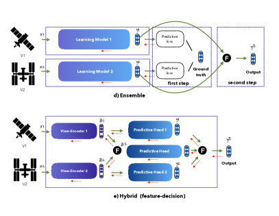
(a)

(b)

Figure 1: MVL fusion strategies compared in this manuscript. The first three (a, b, c) are the main fusion strategy distinctions made in the literature. The “learning model” includes an encoder followed by a prediction head. Green arrows represent the forward pass of the models (left to right), while red arrows represent the backward pass.

We use common-choices of fusion strategies for MVL models [Ofori-Ampofo et al., 2021, Hong et al., 2021, Sainte Fare Garnot et al., 2022, Mena et al., 2024a]: input-level fusion (Input in short), feature-level fusion (Feature in short), decision-level fusion (Decision in short), ensemble-based aggregation (Ensemble in short), and hybrid fusion (Hybrid in short). An illustration of these methods for a two-view learning is presented in Fig. 1.

Input fusion

This strategy concatenates the input views and feeds them to a single model for prediction (with an encoder and a prediction head). As the input views might have different resolutions, an alignment step is usually required to match all the view dimensions, e.g. spatio-temporal alignment using re-sampling or interpolation operations. Considering the multi-view data and the function composition operator $\circ$, this strategy is expressed for the $i$-th sample by

$$\mbox{{X\/}}_{F}^{(i)} ={\mbox{{merge}}}\left({\mbox{{alignment}}}(\left\{\mbox{{X\/}}_{v}^{(i)}\right\}_{v\in\mathcal{V}})\right),$$ (1)

$$\hat{y}^{(i)} ={\mbox{{P}}}_{F}\circ{\mbox{{E}}}_{F}(\mbox{{X\/}}_{F}^{(i)}).$$ (2)

Feature fusion

This strategy uses view-encoders that map each view to a new high-level feature space. Then, a merge function combines this information, obtaining a single high-level joint representation. At last, a prediction head is included to generate the final prediction. Considering the multi-view scenario, this is expressed for the $i$-th sample by

$$\mbox{{z}}_{v}^{(i)} ={\mbox{{E}}}_{v}(\mbox{{X\/}}_{v}^{(i)})\ \ \forall v\in\mathcal{V},$$ (3)

$$\mbox{{z}}_{F}^{(i)} ={\mbox{{merge}}}\left(\left\{\mbox{{z}}_{v}^{(i)}\right\}_{v\in\mathcal{V}}\right),$$ (4)

$$\hat{y}^{(i)} ={\mbox{{P}}}_{F}(\mbox{{z}}_{F}^{(i)}).$$ (5)

Decision fusion

This strategy utilizes parallel models for each view (with a view-encoder and a view-prediction head). These view-dedicated models generate individual decisions (the crop probability) that are merged to yield the aggregated prediction, similar to a mixture of experts technique [Masoudnia and Ebrahimpour, 2014]. Considering the multi-view data, this is expressed by

$$y_{v}^{(i)} ={\mbox{{P}}}_{v}\circ{\mbox{{E}}}_{v}(\mbox{{X\/}}_{v}^{(i)}),\ \ \forall v\in\mathcal{V},$$ (6)

$$\hat{y}^{(i)} ={\mbox{{merge}}}\left(\left\{y_{v}^{(i)}\right\}_{v\in\mathcal{V}}\right).$$ (7)

Ensemble aggregation

Similarly to Decision fusion, this strategy merges the information from the last layer of parallel models, but on a two-step basis. The first step (learning) corresponds to training a model for each view without fusion, while the second step (inference) aggregates the predicted probabilities from the trained view-dedicated models. While the Decision strategy learns the view-dedicated models through the same optimization framework, $\min_{\left\{{\mbox{{P}}}_{v},{\mbox{{E}}}_{v}\right\}_{v\in\mathcal{V}}}{\mbox{{L}}}(y^{(i)},\hat{y}^{(i)})$, the Ensemble learns the models individually, $\min_{{\mbox{{P}}}_{v},{\mbox{{E}}}_{v}}{\mbox{{L}}}(y^{(i)},y_{v}^{(i)})$. The Ensemble strategy does not optimize or learn over the fusion.

Hybrid fusion

This strategy combines some previous fusion strategies in the same MVL model. For instance, we consider the Hybrid fusion with a feature and decision-level mix. This could be seen as two MVL models with shared view-encoders and one final aggregation of their predictions, expressed for the $i$-th sample by

$$\mbox{{z}}_{v}^{(i)} ={\mbox{{E}}}_{v}(\mbox{{X\/}}_{v}^{(i)})\ \ \forall v\in\mathcal{V},$$ (8)

$$y^{(i,\text{feature})} ={\mbox{{P}}}^{\text{feature}}_{F}\circ{\mbox{{merge}}}\left(\left\{\mbox{{z}}_{v}^{(i)}\right\}_{v\in\mathcal{V}}\right),$$ (9)

$${y}^{(i,\text{decision})} ={\mbox{{merge}}}\left(\left\{{\mbox{{P}}}_{v}^{\text{decision}}(\mbox{{z}}_{v}^{(i)})\right\}_{v\in\mathcal{V}}\right),$$ (10)

$$\hat{y}^{(i)} ={\mbox{{merge}}}\left(y^{(i,\text{feature})},{y}^{(i,\text{decision})}\right).$$ (11)

Beyond the conceptual advantages of each fusion strategy, as further detailed in Mena et al. [Mena et al., 2024a], there is an important difference in the number of parameters of the models. For simplicity, let $n_{E}$ be the number of learnable parameters in the encoder E (assuming all view-encoders have the same) and $n_{P}$ the number of parameters in the prediction head P (assuming all view-prediction heads have the same). Then, using a pooling merge function, i.e. a merge function that keeps the same dimensionality of individual representations (e.g. average), the total number of parameters for each MVL model with different fusion strategies are: $n_{E}+n_{P}$ for Input, $|\mathcal{V}|\cdot n_{E}+n_{P}$ for Feature, $|\mathcal{V}|\cdot(n_{E}+n_{P})$ for Decision and Ensemble, and $|\mathcal{V}|\cdot(n_{E}+n_{P})+n_{P}$ for Hybrid strategies.

3.4 Additional Components

Different components can be incorporated into the previous MVL models. In this work, we consider two options that can only be included with the Feature, Decision and Hybrid strategies. The first one is gated fusion (or G-Fusion in short, [Mena et al., 2024b]), a method that adaptively merges learned representations ($\mbox{{z}}_{v}^{(i)}$ or $y_{v}^{(i)}$) through a weighted sum, ${\mbox{{merge}}}(\{\mbox{{z}}_{v}^{(i)}\}_{v\in\mathcal{V}})=\sum_{v\in\mathcal{V}}\bm{\alpha}_{v}^{(i)}\odot\mbox{{z}}_{v}^{(i)}$. The weights $\bm{\alpha}_{v}^{(i)}$ have the same dimension as the learned representation (feature-specific weight) and are computed for each sample based on a gated unit, ${\alpha}^{(i)}={\mbox{{GU}}}(\{\mbox{{X\/}}_{v}^{(i)}\}_{v\in\mathcal{V}})$. We use the learned representations of the view-dedicated models as input for the gated unit [Mena et al., 2024b]. The second is multiple losses (or Multi-Loss in short, [Benedetti et al., 2018]); this method includes one loss function for each view-specific prediction $\hat{y}_{v}^{(i)}$, to force the model to predict the target based on the individual information. These loss functions are added with a weight $\gamma$ to the function to be optimized: ${\mbox{{L}}}(y^{(i)},\hat{y}^{(i)})+\gamma\sum_{v\in\mathcal{V}}{\mbox{{L}}}(y^{(i)},\hat{y}_{v}^{(i)})$. We use the value from the original proposal [Benedetti et al., 2018], $\gamma=0.3$. For the Feature fusion, auxiliary view-prediction heads need to be included to generate the view-specific predictions: $\hat{y}_{v}^{(i)}={\mbox{{P}}}_{v}^{\text{auxiliary}}(\mbox{{z}}_{v}^{(i)})$.

4 Data

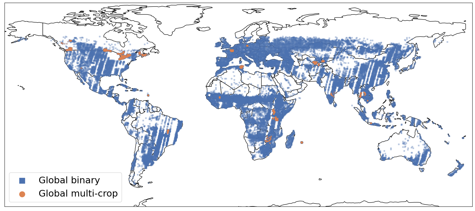
Figure 2: Spatial coverage of the CropHarvest dataset. The blue square markers are the samples with binary labels (all global data), while the orange circular markers are the subset that has multiple crop-type labels (multi-crop subset).

Table 1: Number of samples per year and continent in the CropHarvest data. NA/SA are abbreviations for North/South America.

Year	2016	2017	2018	2019	2020	2021
Samples	27245	6418	5775	11388	6224	8195
Continent	Africa	Asia	Europe	NA	Oceania	SA
Samples	16633	11039	19446	10656	756	6715

Data description

The case study corresponds to crop identification, i.e., predicting a specific crop’s presence or absence in a particular coordinate. For this objective, multiple RS data sources are available as input data to detect if the target crop is cultivated in a geographic region. We use the CropHarvest dataset for a pixel-wise crop classification [Tseng et al., 2021]. This dataset consists of globally (and sparsely) distributed data points across the Earth between 2016 and 2021, see Fig. 2 for the spatial coverage. These data points correspond to 65245 samples that are harmonized between points and polygons into a 100 $m^{2}$ region each (10 meters per pixel of spatial resolution), please refer to [Tseng et al., 2021] for a description of this process. We filtered out samples that did not have associated RS data for prediction. The number of samples per year and continent are shown in Table 1. The data per country is illustrated in Fig. 3a, where it can be seen a long-tail distribution, with almost half of the countries with less than 50 samples. The five countries with the higher number of samples in descending order are France, Canada, Brazil, Uzbekistan, and Germany, while the countries with fewer data are from Asia. We selected this dataset for its global-scale and large variability that reflect different points of view in the analysis.

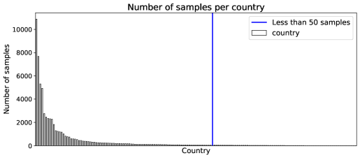
(a) Data points per country in the Global Binary scenario.

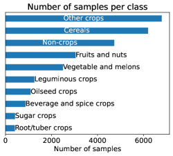
(b) Data points per crop-type in the Global Multi-crop scenario.

Figure 3: Number of samples in the CropHarvest data according to each country and classes (crop-type).

Table 2: Number of samples in each evaluation scenario. The percentage of positive labeled data for the binary classification is shown in parentheses. In Kenya this corresponds to the percentage of maize crops, in Brazil the coffee crops, while in Togo and Global Binary is any crop.

Data	Training samples	Testing samples
Kenya	1319 ($20.0\%$)	898 ($64.0\%$)
Brazil	1583 ($1.00\%$)	537454 ($32.4\%$)
Togo	1290 ($55.0\%$)	306 ($34.6\%$)
Global Binary	45725 ($66.4\%$)	19520 ($66.0\%$)
Global Multi-crop	19066       (—)	8142       (—)

Evaluation scenarios and target task

The dataset provides three geographical regions, with the corresponding training and testing data, as benchmark for binary (cropland) classification. The tasks are to identify maize from other crops (maize vs the rest) in Kenya, coffee crops in Brazil, and distinguish between crop vs non-crop in Togo. Additionally, we create two scenarios considering data from all the countries. The first scenario, Global Binary, uses all the data for crop vs. non-crop classification, i.e. cropland classification, while the second scenario, Global Multi-crop, uses only the subset of samples that have labels with greater granularity (9 groups of crop-types and one non-crop) for a multi-class (crop-type) classification. The classes and data distribution for the latter scenario are depicted in Fig. 3b. The multi-crop is a subset of the binary set because not all samples have this finer label granularity. Table 2 displays the distribution of training and testing samples for each evaluation scenario. For the global scenarios, we randomly selected 30% of the data for testing.

Multi-view input data

Each labeled sample has five views available as input data from four RS sources: S2, S1, ECMWF Reanalysis v5 (ERA5), and Shuttle Radar Topography Mission (SRTM). The optical view is a multi-spectral optical SITS with 11 bands from the S2 mission at 10-60 m/px spatial resolution and approximately five days of revisiting time. The optical view provides the main information on the crop’s composition, growth stage, canopy structure, and leaf water content [Tseng et al., 2021]. The radar view is a 2-band (VV and VH polarization) radar SITS from the S1 mission at 10 m/px and a variable revisit time. The radar view could penetrate cloud cover and provide information about the geometry and water content of the crop. The weather view is a 2-band (precipitation and temperature) time series from the ERA5 at 31 km/px and hourly temporal resolution. The weather view provides information about the expected crop development based on the climate conditions. The NDVI view, which provides information about healthy and dense vegetation, is calculated from the optical view. These temporal views were monthly re-sampled over one year, i.e. 12 steps time series. The static information of elevation and slope is also included as a topographic view, coming from the SRTM’s digital elevation model at 30 m/px. The topographic view can provide information about the suitability of certain crops. The input views in the benchmark were spatially interpolated to a 10 m/px for a pixel-wise mapping, see [Tseng et al., 2021] for further details.

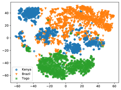
Figure 4: Manifold visualization of the three evaluation countries in the CropHarvest dataset. The t-SNE method is used to generate a 2D projection from the concatenation of the available multi-view input data.

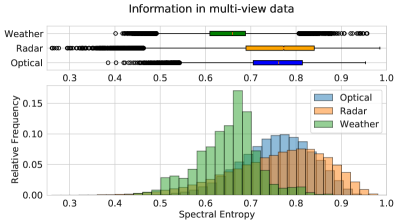
(a) Global data.

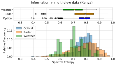
(b) Kenya data.

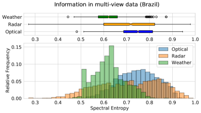
(c) Brazil data.

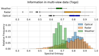
(d) Togo data.

Figure 5: Boxplot and histogram of the spectral entropy (proxy to non-periodic patterns) of the temporal views across the different scenarios.

Descriptive analysis

A visualization of the training data from the three evaluation countries is presented in Fig. 4. Here, the t-distributed Stochastic Neighbor Embedding (t-SNE, [Van der Maaten and Hinton, 2008]) method is used to obtain a projection based on the flattened version of the multi-view data. Even though the separation between points from different regions is not perfect, most of the samples from the same region are clustered together, suggesting a region-dependent behavior in the input data. Additionally, we visualize the time series information of the optical, radar, and weather views in Fig. 5. For this, the spectral entropy across the signal [Inouye et al., 1991] is calculated as a proxy to information level, i.e. a higher value means a signal with more information or non-periodic patterns while a lower value means a constant-like or periodic-behavior signal. We calculated the mean of the spectral entropy across the features in each view. This shows that a-priori, the weather view is the one with less information, and that the radar view is the one with more non-periodic patterns. In addition, the views on the Brazil data show a bit lower entropy values.

5 Experiments

5.1 Evaluation Settings

Table 3: Number of learnable parameters of NN architectures (view-encoders and prediction head) for different views.

	LSTM	GRU	TAE	l-TAE	CNN	MLP
Optical	57152	43904	56598	19350	258880	-
Radar	54592	42176	56004	18756	256000	-
Weather	54592	42176	56004	18756	256000	-
NDVI	50688	41984	55938	18690	255680	-
Topogr.	-					4352
Prediction head						20802

We assess the different MVL models (involving the encoder architectures and fusion strategies), repeating each experiment 20 times and reporting the metrics average with the standard deviation in the testing data. We use three metrics to assess the predictive quality in the classification task: average accuracy (AA), Kappa score ($\kappa$), and F1 macro score ($F_{1}^{\text{macro}}$):

AA $$=\frac{1}{K}\sum_{k\in[K]}\frac{TP_{k}+TN_{k}}{TP_{k}+FN_{k}+TN_{k}+FP+k},$$ (12)

$$\kappa =\frac{2\cdot(TP\cdot TN-FN\cdot FP)}{(TP+FP)\cdot(FP+TN)+(TP+FN)\cdot(FN+TN)},$$ (13)

$$F_{1}^{\text{macro}} =\frac{1}{K}\sum_{k\in[K]}2\frac{P_{k}\cdot R_{k}}{P_{k}+R_{k}},$$ (14)

with $TP_{k}$ the false positive rate, $FN_{k}$ the false negative rate, $TN_{k}$ the true positive rate, $FP_{k}$ the false positive, $P_{k}$ the precision, and $R_{k}$ the recall, all regarding class $k\in[K]$. The MVL models are optimized over the cross entropy loss with the ADAM optimizer and a 256 batch size. We use an early stopping criterion with 5 tolerance steps on a 10% validation data extracted from the training data. We incorporate class weights, inversely proportional to class frequencies, into the objective function [King and Zeng, 2001]. This approach addresses the class unbalance (Fig. 3b) by ensuring a balanced impact of the samples from each class within the loss function.

We experiment with all the encoder architectures described in Sec. 3.2 for the temporal views (optical, radar, weather, and NDVI), while for the elevation view (static features) we only used an MLP as the view-encoder. We use the NDVI as a separate view as has been shown optimal results in the literature [Audebert et al., 2018, M Rustowicz et al., 2019, Sheng et al., 2020]. For the hyperparameter tuning and selection in each encoder architecture, we did a random exploration of 10 to 50 trials in the Kenya data. The hyperparameters tried for each architecture were the number of layers, the hidden state/features, the use of batch-normalization, in addition to more specific like bidirectional recurrence in GRU and LSTM, number of heads in TAE and L-TAE, and kernel size in TempCNN. We use the configurations suggested in the original papers as the initial guesses of the parameter values (in most of the cases they were the best). The reason to do the selection in Kenya data is because it was the focus of the Agriculture-vision competition and it is the more challenging evaluation scenario. It is important to note that we selected the same encoder architecture for all the temporal views across the different model configurations, i.e. we did not test combinations such as LSTM for optical and GRU for radar. Among the common selected hyperparameters in the view-encoders are: 64 dimensions in the hidden state/features with two layers, and 64 dimensions in the embedding vector. The prediction head is the same for all fusion strategies, an MLP with a single hidden layer of 64 units and batch-normalization layer. For further regularization, we use 20% of dropout. In Table 3 we compare the number of parameters of the different encoder architectures depending on the input view.

Throughout our experiments, we incorporated an SVL baseline composed of a NN (encoder and prediction head) trained using a single-view as input data. We report the results of the SVL model with the optical or radar view, selecting the one that yields the most favorable predictions in each case, while the results for both can be found in the appendix A.

5.2 Class Prediction Results

Table 4: Crop classification results on the country-specific evaluation. Here, we only report the view-encoders architecture which yielded the best results in each fusion strategy. The mean $\pm$ standard deviation between 20 training repetitions is shown. The metrics are scaled between 0 and 100. We highlight the first and second highest metrics in each country.

Country	Fusion Strategy	View-Encoder	Component	AA	Kappa ($\kappa$)	$F_{1}^{\text{macro}}$
Kenya	single-view	TempCNN	Radar view	${{\color[rgb]{0,0,1}\mathbf{{67.61\pm 1.19}}}}$	${{\color[rgb]{0,0,1}\mathbf{{39.68\pm 3.40}}}}$	${{\color[rgb]{0,0,1}\mathbf{{68.44\pm 1.56}}}}$
	Input	TAE	-	${\mathbf{{67.25\pm 5.48}}}$	${\mathbf{{37.04\pm 11.41}}}$	${\mathbf{{67.15\pm 7.80}}}$
	Feature	LSTM	-	${64.38\pm 7.24}$	$28.92\pm 14.94$	$62.47\pm 11.03$
	Decision	GRU	G-Fusion	$63.73\pm 6.21$	${29.81\pm 13.67}$	${63.59\pm 7.27}$
	Hybrid	LSTM	-	$61.32\pm 7.04$	$24.51\pm 14.98$	$59.00\pm 11.39$
	Ensemble	LSTM	-	$55.86\pm 5.88$	$13.68\pm 13.49$	$50.62\pm 10.08$
Brazil	single-view	TAE	Optical view	$97.03\pm 1.98$	$93.44\pm 4.94$	$96.71\pm 2.50$
	Input	GRU	-	$95.59\pm 3.67$	$92.52\pm 6.18$	$96.25\pm 3.12$
	Feature	LSTM	-	${{\color[rgb]{0,0,1}\mathbf{{97.50\pm 1.43}}}}$	${{\color[rgb]{0,0,1}\mathbf{{95.77\pm 2.53}}}}$	${{\color[rgb]{0,0,1}\mathbf{{97.88\pm 1.27}}}}$
	Decision	LSTM	Multi-Loss	$94.91\pm 7.17$	$91.67\pm 12.58$	$95.73\pm 6.68$
	Hybrid	LSTM	-	${\mathbf{{97.38\pm 2.35}}}$	${\mathbf{{95.64\pm 3.79}}}$	${\mathbf{{97.81\pm 1.90}}}$
	Ensemble	TempCNN	-	$80.28\pm 14.17$	$59.70\pm 30.41$	$76.01\pm 22.27$
Togo	single-view	GRU	Optical view	$80.33\pm 1.78$	$55.94\pm 4.44$	$77.55\pm 2.49$
	Input	GRU	-	$80.48\pm 1.42$	$56.18\pm 3.72$	$77.66\pm 2.09$
	Feature	GRU	-	$79.09\pm 1.35$	$53.50\pm 3.17$	$76.30\pm 1.79$
	Decision	GRU	Multi-Loss	${\mathbf{{82.52\pm 1.58}}}$	${\mathbf{{59.82\pm 3.89}}}$	${\mathbf{{79.52\pm 2.14}}}$
	Hybrid	GRU	-	$80.00\pm 6.50$	$55.66\pm 12.48$	$76.56\pm 10.49$
	Ensemble	GRU	-	${{\color[rgb]{0,0,1}\mathbf{{84.15\pm 1.59}}}}$	${{\color[rgb]{0,0,1}\mathbf{{64.43\pm 4.35}}}}$	${{\color[rgb]{0,0,1}\mathbf{{82.03\pm 2.32}}}}$

Table 5: Crop classification results on the global evaluation. The best combination of view-encoders architecture is selected for each fusion strategy. The mean $\pm$ standard deviation between 20 training repetitions is shown. The metrics are scaled between 0 and 100. We highlight the first and second highest metrics in each country.

Data	Fusion Strategy	View-Encoder	Component	AA	Kappa ($\kappa$)	$F_{1}^{\text{macro}}$
Global Binary	single-view	TempCNN	Optical view	$79.98\pm 0.69$	$55.05\pm 1.30$	$77.15\pm 0.69$
	Input	TempCNN	-	$82.19\pm 0.73$	$59.97\pm 1.61$	$79.76\pm 0.86$
	Feature	TempCNN	G-Fusion	${{\color[rgb]{0,0,1}\mathbf{{83.74\pm 0.53}}}}$	${{\color[rgb]{0,0,1}\mathbf{{63.64\pm 0.93}}}}$	${{\color[rgb]{0,0,1}\mathbf{{81.68\pm 0.47}}}}$
	Decision	TempCNN	-	$82.70\pm 0.61$	$62.20\pm 1.03$	$80.99\pm 0.52$
	Hybrid	TempCNN	G-Fusion	${\mathbf{{83.55\pm 0.81}}}$	${\mathbf{{63.43\pm 1.55}}}$	${\mathbf{{81.58\pm 0.79}}}$
	Ensemble	TempCNN	-	$80.85\pm 0.58$	$56.63\pm 1.08$	$77.95\pm 0.57$
Global Multi-Crop	single-view	TempCNN	Optical view	$67.95\pm 0.70$	$60.80\pm 0.77$	$59.30\pm 0.80$
	Input	TempCNN	-	$69.75\pm 0.96$	$62.57\pm 1.10$	$61.18\pm 1.31$
	Feature	TempCNN	G-Fusion	${{\color[rgb]{0,0,1}\mathbf{{71.11\pm 0.88}}}}$	${\mathbf{{64.85\pm 1.25}}}$	${\mathbf{{63.47\pm 1.38}}}$
	Decision	TempCNN	-	$70.35\pm 0.74$	$64.15\pm 1.35$	$62.69\pm 1.44$
	Hybrid	TempCNN	G-Fusion	${\mathbf{{70.70\pm 0.48}}}$	${{\color[rgb]{0,0,1}\mathbf{{64.99\pm 0.99}}}}$	${{\color[rgb]{0,0,1}\mathbf{{63.56\pm 1.16}}}}$
	Ensemble	TempCNN	-	$67.54\pm 0.54$	$58.35\pm 0.92$	$56.47\pm 0.93$

The first research question we explore is how does the decision of the encoder architecture and fusion strategy affect the correctness of the MVL model predictions? To address this, we tested the five encoder architectures described in Sec. 3.2 in the five fusion strategies described in Sec. 3.3, including the two components described in Sec. 3.4 for the Feature, Decision and Hybrid strategies. This resulted in 31 experiments ($5\cdot 5+2\cdot 3$) that we repeated 20 times. The results for the country-specific evaluation are shown in Table 4, and for the global in Table 5.

Overall, we observe that the SVL classification results were outperformed by the MVL models in different amounts depending on the metric and evaluation scenario. For instance, compared to the SVL results, the AA increased around $0.5$ points in Brazil, from $97.03$ to $97.50$, and $4$ points in the global evaluation, while the $\kappa$ score increased around $2$ points in Brazil and $8$ points in the Global Binary, from $55.05$ to $63.64$. As a common result in the literature, this suggests that additional RS sources help improve the classification task’s predictive quality. However, there is an exception in Kenya, where the LSTM view-encoder with the radar view obtains the best predictions, we discuss this a bit further in Sec. 6. Regarding the country-specific evaluation (in Table 4), we notice that the Decision fusion is the only strategy that improves its predictions by using additional components (the results with all the components could be found in the Table A1 in the appendix). Additionally, some model combinations produce very unstable results with a high prediction variance. For instance, LSTM view-encoders with Feature and Hybrid in Kenya, TempCNN view-encoders with Ensemble in Brazil, and GRU view-encoders with Hybrid in Togo. This behavior is expected due to the limited amount of data available for training (see Table 2). Because the best predictive quality is achieved with a different model configuration in each country, and due to the high variance behavior with some configurations, it is evident that in local scenarios with a few labeled samples, model selection is crucial.

In the results of the global evaluation (Table 5) we observe a clear difference between the multi-class and binary classification. This reflects the challenge of a fine-grained classification involving multiple crops with respect to a binary cropland classification. In these experiments, the gated fusion component manages to improve its predictions in some fusion strategies, as opposite to the country-specific evaluation where only in Decision and Kenya data was useful. Besides, the variance in the model results is much lower than in the country-specific, as we expected due to the greater number of labeled training samples. With each fusion strategy, the best classification results in the global evaluation are obtained with the TempCNN. We suspect that is because the global datasets have more training samples to properly learn the more complex TempCNN model (Table 3). Moreover, the best classification results are obtained with the Feature and Hybrid strategies. However, for these kinds of scenarios, we recommend using the Feature fusion strategy because it obtains less complex models (in terms of learnable parameters), and has consistently better results in the country-specific evaluation.

Table 6: Crop classification results when selecting the architecture of the encoders based on the Input fusion strategy. The Togo, and Global evaluation are excluded, since those results can already be found in Table 4 and 5. The mean $\pm$ standard deviation between 20 training repetitions is shown. The metrics are scaled between 0 and 100. We highlight the first and second highest metrics in each country.

Country	Fusion Strategy	View-Encoder	Component	AA	Kappa ($\kappa$)	$F_{1}^{\text{macro}}$
Kenya	Input	TAE	-	${{\color[rgb]{0,0,1}\mathbf{{67.25\pm 5.48}}}}$	${{\color[rgb]{0,0,1}\mathbf{{37.04\pm 11.41}}}}$	${{\color[rgb]{0,0,1}\mathbf{{67.15\pm 7.80}}}}$
	Feature		Multi-Loss	$53.80\pm 5.39$	$8.85\pm 11.49$	$47.00\pm 8.40$
	Decision		-	$53.47\pm 3.85$	$8.13\pm 8.45$	$47.20\pm 7.18$
	Hybrid		G-Fusion	${\mathbf{{57.02\pm 5.69}}}$	${\mathbf{{14.77\pm 11.44}}}$	${\mathbf{{53.34\pm 8.62}}}$
	Ensemble		-	$50.45\pm 0.53$	$1.15\pm 1.30$	$40.26\pm 1.46$
Brazil	Input	GRU	-	$95.59\pm 3.67$	$92.52\pm 6.18$	$96.25\pm 3.12$
	Feature		Multi-Loss	${\mathbf{{96.57\pm 2.22}}}$	${{\color[rgb]{0,0,1}\mathbf{{94.69\pm 3.35}}}}$	${{\color[rgb]{0,0,1}\mathbf{{97.34\pm 1.68}}}}$
	Decision		-	$96.46\pm 4.09$	${\mathbf{{94.27\pm 6.52}}}$	${\mathbf{{97.13\pm 3.30}}}$
	Hybrid		-	${{\color[rgb]{0,0,1}\mathbf{{96.58\pm 2.96}}}}$	$94.22\pm 4.44$	$97.10\pm 2.23$
	Ensemble		-	$70.49\pm 13.15$	$34.61\pm 27.64$	$59.55\pm 19.41$

Moreover, we explore the question of when an encoder architecture is selected in a single fusion strategy, how do the MVL model predictions change when using a different fusion strategy? To address this, we first tried the five encoder architectures only with the Input fusion and selected the one with the best predictive quality. Then, the five fusion strategies are tested with the selected encoder architecture (including the gated fusion and multiple loss variations). This research approach reduces the number of experiments compared to the previous one, concretely to 16 experiments ($5+5+2\cdot 3$). The results are shown in Table 6. Notice that we do not include the Togo and Global results since those could be observed in Table 4 and 5, as all the fusion strategies already have the same encoder architecture. Overall, we identify that the other fusion strategies could indeed improve the predictive quality of the MVL model with Input fusion, except for the Kenya data. In the country-specific evaluation, the $\kappa$ score increases from around 2 points in Brazil by the Feature fusion to around 8 points in Togo by the Ensemble strategy. The global evaluation shows slight increases in the AA and $F_{1}^{\text{macro}}$ of 1 to 2 points by the Feature fusion. Anyhow, based on the reduction of the number of experiments from product ($5\cdot 5$) to sum ($5+5$) and the moderate improvement in the classification results, we consider this approach to be worthwhile for future research.

Lastly, we remark that our results does not outperform the current state-of-the-art in the benchmark countries obtained by Tseng et al. [Tseng et al., 2022, Tseng et al., 2023] with Input fusion and pre-training techniques. Yet, our goal is to provide a comprehensive evaluation of the MVL modeling options for researchers in the field without relying on pre-training approaches.

5.3 Predicted Probabilities Analysis

Table 7: Predicted probability analysis in the country-specific evaluation. The best combination, based on the predictive quality (in Table 4), is shown for each fusion strategy. The single-view in Kenya is radar, while for Brazil and Togo is optical. The mean $\pm$ standard deviation between 20 training repetitions is shown. The metrics are scaled between 0 and 100.

Country	Strategy	View-Encoder	Prediction Entropy	Max. Probability
Kenya	single-view	TempCNN	$42.4\pm 5.9$	$88.8\pm 1.8$
	Input	TAE	$67.1\pm 7.4$	$77.7\pm 3.9$
	Feature	LSTM	$78.5\pm 8.6$	$72.2\pm 5.6$
	Decision	GRU	$74.8\pm 4.0$	$75.2\pm 2.2$
	Hybrid	LSTM	$91.5\pm 4.7$	$63.5\pm 5.4$
	Ensemble	LSTM	$85.3\pm 3.9$	$69.3\pm 2.8$
Brazil	single-view	TAE	$66.2\pm 13.1$	$78.6\pm 6.8$
	Input	GRU	$43.7\pm 19.1$	$87.9\pm 7.8$
	Feature	LSTM	$38.5\pm 16.2$	$90.3\pm 5.8$
	Decision	LSTM	$63.8\pm 11.8$	$79.3\pm 7.7$
	Hybrid	LSTM	$86.3\pm 4.6$	$68.2\pm 3.7$
	Ensemble	TempCNN	$91.9\pm 4.9$	$63.0\pm 5.8$
Togo	single-view	GRU	$63.3\pm 3.0$	$79.3\pm 1.3$
	Input	GRU	$56.9\pm 6.0$	$81.8\pm 2.4$
	Feature	GRU	$55.6\pm 4.7$	$82.2\pm 1.8$
	Decision	GRU	$71.4\pm 3.2$	$76.0\pm 1.4$
	Hybrid	GRU	$90.1\pm 2.3$	$65.8\pm 3.0$
	Ensemble	GRU	$93.7\pm 0.6$	$62.4\pm 0.7$

As a complementary analysis, we explore the question of how does MVL affect the confidence and uncertainty of model predictions? To answer this, we compute two measures commonly used to quantify uncertainty [Malinin and Gales, 2018]. These are independent of the target labels and only use the probability predictions of a MVL model, $\hat{y}^{(i)}_{k}=\hat{p}(y=k|\mathcal{X}^{(i)})$. The max. probability measuring the model’s confidence on the predicted class, $\frac{1}{N}\sum_{i=1}^{N}\max_{k}\hat{y}^{(i)}_{k}$, and the prediction entropy measuring the classification uncertainty of the model prediction, $-\frac{1}{N}\sum_{i=1}^{N}\sum_{k=1}^{K}\hat{y}^{(i)}\log{\hat{y}_{k}^{(i)}}$. Table 7 displays the results in the country-specific evaluation using the best model configuration in the classification results. We do not report the results on the global datasets since they exhibit similar patterns. We notice that a model with high max. probability and low prediction entropy obtains the best classification results, such as Feature fusion in Brazil, but not in all cases. Surprisingly, sometimes the less confident and more uncertain predictions are generated by the model with the best classification results, such as the Ensemble strategy in Togo. This high uncertainty prediction pattern is associated with the most complex models (Hybrid) or the ones that do not learn to fuse (Ensemble). Additionally, since we employ the early stopping criteria, the training can be stopped when a good classification is reached (although the classification is not so confident in terms of the predicted probability). Similar to what we observed in Mena et al. [Mena et al., 2023] and regardless of the encoder decision, the prediction uncertainty tends to increase slightly as the fusion moves from the input to the output layers of the MVL model.

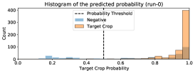
(a) Radar with TempCNN.

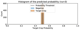
(b) Hybrid with LSTM.

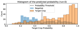
(c) Input with TAE.

Figure 6: Distribution of the probability predicted by different models in Kenya. The values are taken from a single run with a) SVL model, b) MVL model with high prediction uncertainty, and c) MVL model with low prediction uncertainty.

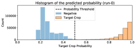
(a) Optical with TAE.

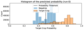
(b) Ensemble with TempCNN.

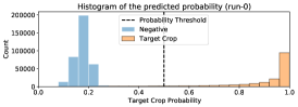
(c) Feature with LSTM.

Figure 7: Distribution of the probability predicted by different models in the testing data of Brazil. The values are taken from a single run with a) SVL model, b) MVL model with high uncertainty, and c) MVL model with uncertainty.

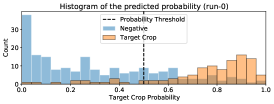
(a) Optical with GRU encoder.

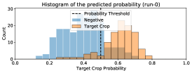
(b) Ensemble with GRU view-encoders.

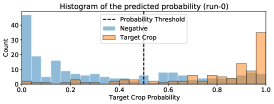
(c) Feature with GRU view-encoders.

Figure 8: Distribution of the probability predicted by different models in the testing data of Togo. The values are taken from a single run with a) SVL model, b) MVL model with high uncertainty, and c) MVL model with uncertainty.

Finally, as a qualitative analysis, we include some charts with the probability distribution associated to the positive label in the country-specific evaluation (of a single run). In Figure 6, 7, and 8 we display this for each country. We select the SVL model, the MVL model with most uncertain predictions, and the MVL model with most confident predictions. These plots help to interpret the previous quantities from Table 7. Here, a probability prediction closer to the decision boundary of 0.5 (indicating more uncertain predictions) carries a high prediction entropy, while a probability prediction in the extremes (0 or 1, and indicating more certain predictions) carries a low prediction entropy. Since the best MVL model assigns more distinguished values (more separated) to the classes compared to the SVL model, it reflects the advantages of using a MVL approach in the modeling.

5.4 Global Dataset Analysis

At last, we explore the question of what data patterns can we observe in the MVL model predictions? To address this, we provide a detailed analysis of the predictive quality of the best MVL model over different data perspectives, such as crop-types, years and continents. To extract significant insights, we selected the MVL model with the best classification results in the global evaluation, which is the Feature fusion with TempCNN view-encoders and G-Fusion component.

Table 8: Crop-wise classification results on the Global Multi-crop evaluation. The mean $\pm$ standard deviation between 20 training repetitions is shown scaled between 0 and 100.

Crop-type ($k$)	$F_{1,k}$	Precision ($P_{k}$)	Recall ($R_{k}$)
Cereals	$83.26\pm 1.31$	$77.08\pm 2.62$	$90.60\pm 1.19$
Others	$75.09\pm 1.14$	$66.00\pm 2.21$	$87.17\pm 1.26$
Non-crop	$72.57\pm 1.13$	$71.55\pm 2.55$	$73.73\pm 1.87$
Leguminous	$70.32\pm 2.78$	$78.86\pm 4.01$	$63.63\pm 3.81$
Oil seeds	$66.07\pm 3.18$	$70.62\pm 3.04$	$62.28\pm 4.90$
Fruits and nuts	$64.81\pm 2.14$	$67.22\pm 4.51$	$62.81\pm 2.60$
Vegetable-melons	$60.40\pm 1.81$	$58.78\pm 3.61$	$62.31\pm 2.20$
Sugar	$58.85\pm 5.01$	$84.82\pm 2.81$	$45.47\pm 6.36$
Root/tuber	$46.48\pm 3.82$	$74.84\pm 3.40$	$33.97\pm 4.40$
Beverage and spice	$36.86\pm 3.28$	$61.35\pm 2.57$	$26.53\pm 1.20$

Table 8 displays the $F_{1}$, precision and recall scores for assessing the individual predictive quality for the 10 crop-types in the data. It can be seen that the class predictions with the lowest $F_{1}$ score (and harder to predict by the model) are “beverage and spices” and “root/tuber” crop-types, mainly due to a low Recall, i.e. the model fails to identify correctly the samples labeled with those crop-types. This could be explained by the fact that these crop-types are among the classes with the least number of samples (see Fig. 3b). On the other hand, the class predictions with higher $F_{1}$ score (and easier to predict by the model) are “cereals” and “others” crop-types, affected mainly by high Recall rather than high Precision, i.e. the model identify correctly most of the samples labeled with those crop-type. Similarly to the crop-types with the lowest $F_{1}$ scores, this could be related to the high number of samples in the “cereals” and “others” crop-types. This pattern could be an effect of model learning in the data, since we did not include any balancing techniques or class weights during training.

Table 9: Year-wise classification results on the Global Binary evaluation. The mean $\pm$ standard deviation between 20 training repetitions is shown scaled between 0 and 100.

Year	AA	Kappa ($\kappa$)	$F_{1}^{\text{macro}}$
2016	$76.97\pm 0.60$	$51.01\pm 1.09$	$75.06\pm 0.56$
2017	$85.82\pm 2.33$	$72.65\pm 2.37$	$86.63\pm 1.20$
2018	$93.78\pm 0.51$	$78.25\pm 0.75$	$89.08\pm 0.38$
2019	$76.61\pm 1.72$	$49.17\pm 2.00$	$74.50\pm 1.02$
2020	$89.76\pm 1.53$	$81.60\pm 2.18$	$90.79\pm 1.10$
2021	$87.51\pm 0.50$	$67.21\pm 1.61$	$83.33\pm 0.89$

Table 10: Continent-wise classification results on the Global Binary evaluation. The mean $\pm$ standard deviation between 20 training repetitions is shown scaled between 0 and 100.

Continent	AA	Kappa ($\kappa$)	$F_{1}^{\text{macro}}$
Africa	$75.09\pm 1.20$	$53.44\pm 2.22$	$76.07\pm 1.24$
Asia	$86.68\pm 0.47$	$64.97\pm 1.01$	$82.33\pm 0.54$
Europe	$79.49\pm 0.70$	$54.18\pm 0.90$	$76.95\pm 0.46$
NA	$83.26\pm 1.46$	$61.98\pm 1.61$	$80.92\pm 0.80$
Oceania	$77.67\pm 2.48$	$52.42\pm 5.35$	$75.69\pm 3.03$
SA	$86.87\pm 1.46$	$69.34\pm 1.83$	$84.61\pm 0.91$

In addition, we present the classification results in each continent and year for the Global Binary evaluation. Table 10 presents the AA, $\kappa$ and $F_{1}^{\text{macro}}$ score for assessing the predictive quality in each year, while Table 10 shows the same results aggregated per continent. The best results of AA are obtained from the 2018 data, which also yields the second-best $\kappa$ and $F_{1}^{\text{macro}}$. One reason could be that machine learning models are good interpolators and there is enough information in the training data to learn about the past (pre-2018) and future (post-2018). Nevertheless, there could be a relation with the number of samples (Table 2), since the best results of $\kappa$ and $F_{1}^{\text{macro}}$ are found in the year 2020, the second year with the least amount of data after 2018. In contrast, the years 2016 and 2019, the years with the largest number of samples, are exhibiting the worst scores. There is a similar behavior in the continent-perspective, where the worst AA results are found in Africa, despite being the continent with the second-largest number of samples. Surprisingly, in the continent with the largest number of samples, Europe, the classification results are quite similar to the bad ones obtained in Africa. On the other side, the best classification results are in South America and Asia continents. The top results in South America are interesting because it is the second continent with fewer number of samples.

Figure 9: Predicted data points in the Global Binary evaluation. Red crosses are points with the predicted class equals to the target class, while green circles are samples with the predicted class different from the target.

Furthermore, we display the prediction errors of the training and testing data on a map to illustrate the mistakes of the model predictions geographically. To obtain a single prediction of each data point, the best model is selected between the 20 repetitions. This is presented in Fig. 9, where to highlight errors, we put them in the foreground. We created the same plots for the other methods and presented them in the appendix B, as well as a heatmap error per country. As depicted in Table 10, most of the prediction errors come from the Africa continent, especially in the north of the equator, such as in West Africa. In contrast, there are fewer prediction errors in South America and Asia. Nevertheless, it can be seen that there are no unique error patterns in localized regions, rather the model makes errors in different zones of the world.

6 Discussion

In this section, we address some key points that are relevant to our empirical evidence.

Challenging evaluation scenario in Kenya

As we present in our study, there are some negative exceptions in the results when looking at Kenya data. Therefore, we ask why is there such a different behavior in the Kenya data? In Kenya, the weather view has entropy values dispersed over a broader range of values compared to the narrow values in the other countries (Fig. 5). Besides, the radar view in Kenya has slightly more entropy than the other views, relative to the other countries. This could explain why the best SVL model is obtained with the radar view instead of the optical (see Table A1 in the appendix). Additionally, Kenya is the country with the highest number of low outliers in the spectral entropy, among the three countries (Fig. 5), meaning it contains “irregular” samples with non-informative patterns. These can suggest why this evaluation is more difficult than the others and that the best classification model relies on the highest entropy view (radar data), or on a simple fusion strategy with an advanced encoder (Input fusion with TAE encoder). However, when the SVL model with the radar view uses the same encoder architecture as the Input Fusion, the TAE encoder, the classification results are improved by MVL models (see Table A3 in the appendix). This suggests that the better prediction behavior of the SVL model compared to the MVL models may only be circumstantial for the model configuration and the data. Nevertheless, there is evidence in other RS-based applications where fewer data sources are somehow better for the predictive task, such as in crop yield prediction [Kang et al., 2020, Pathak et al., 2023].

Fusion strategy selection based on number of samples

When training with a high number of labeled samples, such as our global scale evaluation (with more than $19$ thousand samples, see Table 2), the predictive quality of the compared MVL models tends to become similar. The difference in the classification results between the best fusion methods is negligible, making the selection of the best fusion strategy less critical. However, with a limited number of training samples, the choice of the most suitable model has a significant impact on the overall predictive quality, emphasizing the need for a careful model selection. When training with few labeled samples like our local scale (country-specific) evaluation (with less than $1.6$ thousand samples), it is more beneficial to use specialized models that are tailored to the specific data. The behavior that the optimal fusion strategy depends on the dataset and region has been observed in both, the RS domain [Masolele et al., 2021, Sainte Fare Garnot et al., 2022, Mena et al., 2023] and the computer vision domain [Ma et al., 2022].

Disadvantages of selecting the encoder with the Input fusion

When the encoder architecture is selected based on the Input fusion, we wonder how much worse the prediction of the MVL models are by limiting the encoder in this selection? In Togo, Global Binary, and Global Multi-crop, the prediction does not get worse since the best classification results of the MVL models with alternative fusion strategies are obtained with the same view-encoders architecture as the Input fusion (GRU, TempCNN, and TempCNN encoder respectively). In Brazil data, the quality of the predictions worsens slightly. When using the encoder architecture selected from the Input fusion, the GRU encoder, the metrics from all the fusion strategies are reduced in around 1 pp. compared to using the best view-encoders in each fusion strategy. In Kenya data, the predictive quality worsens significantly. For instance, focused on the AA results, the second-best fusion strategy, the Feature fusion, reduced the values in around 11 pp. from LSTM (the best view-encoders architecture for Feature) to TAE (the best encoder architecture for Input). Furthermore, the second-best fusion strategy for the $\kappa$ score, the Decision strategy, reduces the values in around 22 pp. from GRU to TAE view-encoders. Nevertheless, in most cases the predictions do not vary much and the number of experiments in this approach is significantly reduced. Therefore, instead of searching for the best view-encoders architecture for each fusion strategy individually, start by finding the best encoder architecture for the Input fusion, and then focus on selecting the optimal fusion strategy.

Fusion strategy recommendation for crop classification

We recommend a fusion strategy in the pixel-wise crop classification task based on all the experiments presented in this manuscript. MVL with the Feature fusion is the strategy with more points in favor. The models generated with this strategy obtain either the best or in the middle classification results across metrics and evaluation scenarios, without being so complex nor so simple in terms of learnable parameters. Besides, these models generate the most confident predictions. Moreover, different MVL components could be incorporated based on the flexibility of NN models [Mena et al., 2024a], such as different fusion mechanisms (gated fusion or probabilistic fusion), regularization constrains (multiple losses or parameter sharing), or modular design (pre-train view-encoders or transfer pre-trained layers). The MVL with Input (and also Ensemble) strategy is a good starting point based on the implementation simplicity and competitive results. However, these strategies are limited to use components for individual models, usually related to the architecture design (e.g. number of layers, types of layers, dropout, batch-normalization), and the evidence reflects that the results can be improved. Our findings and recommendations are further aligned with other results from the literature in crop-related tasks [Cué La Rosa et al., 2018, Ofori-Ampofo et al., 2021, Sainte Fare Garnot et al., 2022], where the Feature fusion strategy obtains either the best or second-best strategy classification results.

7 Conclusion

In this manuscript, we present an exhaustive comparison of MVL models in a pixel-wise crop classification (cropland and crop-type) by varying the view-encoders architecture of temporal views and the fusion strategies between five options each. We assess the predictive quality with different classification metrics in the CropHarvest dataset with various evaluation scenarios. Our main finding is to corroborate the prediction benefits that come from using a model based on multiple RS sources regarding a model based on only one. Besides, we find that for specific regions with limited amount of labeled data, it is better to search for specialized (ideally data dependent) approaches, one model does not fill all. In the search for the best view-encoders architecture and fusion strategy, the search space can be reduced by first searching for the best encoder architecture for only one fusion strategy (we tested with Input fusion), and then searching for the optimal fusion strategy. Within which, we suggest prioritizing the exploration of the Feature fusion strategy due to the different advantages we observed in our experiments. Furthermore, which view or which part of the MVL model contributes more to obtain a better prediction is something that requires further analysis, such as implementing and adapting explainability techniques to MVL. We hope that this work will prove valuable in addressing the challenges posed by MVL and advancing the field of RS-based crop classification.

Limitations

Although the Cropharvest dataset is a harmonization of 20 public crop classification datasets (including DENETHOR - AI4EO Food Security and LEM+ datasets), the results obtained are conditioned to the configuration presented in this dataset. For instance, the re-sampling and interpolation done to obtain the temporal and spatial resolutions, the labeling harmonization process (between polygons and point data), and crop-type classes. We only experimented with different encoder architectures for the temporal views, while the static view was fixed with an MLP encoder. Moreover, additional refinements or changes could be expected if a bigger search space is used when looking for architectures. We are aware that the comparison selection comes with a human bias, and that exist current techniques to search for arbitrary NN architectures using a large amount of computational resources, such as multi-modal neural architecture search. However, our study’s goal is to provide a guided and transparent recommendation for researchers with lower access to computational resources.

Data Availability

Data from the CropHarvest benchmark [Tseng et al., 2021] is used in this paper. The full dataset and documentation can be accessed from https://github.com/nasaharvest/cropharvest.

Abbreviations

The following abbreviations are used in this manuscript:
CNN Convolutional Neural Network ERA5 ECMWF ReAnalysis v5 GRU Gated Recurrent Unit LSTM Long-Short Term Memory L-TAE Lightweight TAE MLP Multi-Layer Perceptron MVL Multi-View Learning NDVI Normalized Difference Vegetation Index NN Neural Network RS Remote Sensing RNN Recurrent Neural Network SAR Synthetic Aperture Radar SRTM Shuttle Radar Topography Mission SITS Satellite Image Time Series SVL Single-View Learning TAE Temporal Attention Encoder TempCNN Temporal CNN

Appendix A Additional Tables

We include an extension of the country-specific results in Table 4 by including all the component and fusion strategy combinations, shown in Table A1. Additionally, we include an extension of the global results from Table 5 in the same way, show in Table A2. Here, we include the AUC ROC metric, which we did not include in the main content since the differences in this metric are insignificant to properly compare. Finally, the same extension is presented from the results in Table 6, shown in Table A3.

Table A1: Crop classification results on the country-specific evaluation, extended from Table 4. Here, we only report the view-encoders architecture which yielded the best results in each fusion strategy. The metrics are scaled between 0 and 100. We highlight the first and second highest metrics in each country.

Country	Fusion Strategy	View-Encoder	Component	AA	Kappa	F1 macro
Kenya	single-view	TempCNN	Optical view	$59.74\pm 2.51$	$20.35\pm 5.39$	$59.47\pm 3.20$
		LSTM	Radar view	$67.61\pm 1.19$	$39.68\pm 3.40$	$68.44\pm 1.56$
	Input	TAE	-	${{\color[rgb]{0,0,1}\mathbf{{67.25\pm 5.48}}}}$	${{\color[rgb]{0,0,1}\mathbf{{37.04\pm 11.41}}}}$	${{\color[rgb]{0,0,1}\mathbf{{67.15\pm 7.80}}}}$
	Feature	LSTM	-	${\mathbf{{64.38\pm 7.24}}}$	$28.92\pm 14.94$	$62.47\pm 11.03$
			Multi-Loss	$62.52\pm 8.91$	$25.43\pm 18.49$	$57.93\pm 16.24$
			G-Fusion	$58.84\pm 7.34$	$18.24\pm 15.04$	$55.31\pm 11.96$
	Decision	GRU	-	$58.66\pm 6.94$	$18.55\pm 15.22$	$58.33\pm 7.63$
			Multi-Loss	$62.28\pm 5.88$	$27.06\pm 12.57$	$61.64\pm 7.57$
			G-Fusion	$63.73\pm 6.21$	${\mathbf{{29.81\pm 13.67}}}$	${\mathbf{{63.59\pm 7.27}}}$
	Hybrid (Feature-Decision)	LSTM	-	$61.32\pm 7.04$	$24.51\pm 14.98$	$59.00\pm 11.39$
			Multi-Loss	$59.55\pm 6.53$	$20.35\pm 13.72$	$56.74\pm 11.16$
			G-Fusion	$59.87\pm 9.57$	$18.22\pm 17.63$	$53.10\pm 14.56$
	Ensemble	LSTM	-	$55.86\pm 5.88$	$13.68\pm 13.49$	$50.62\pm 10.08$
Brazil	single-view	TAE	Optical view	$97.03\pm 1.98$	$93.44\pm 4.94$	$96.71\pm 2.50$
		GRU	Radar view	$64.57\pm 6.77$	$26.64\pm 15.52$	$58.27\pm 11.74$
	Input	GRU	-	$95.59\pm 3.67$	$92.52\pm 6.18$	$96.25\pm 3.12$
	Feature	LSTM	-	${{\color[rgb]{0,0,1}\mathbf{{97.50\pm 1.43}}}}$	${{\color[rgb]{0,0,1}\mathbf{{95.77\pm 2.53}}}}$	${{\color[rgb]{0,0,1}\mathbf{{97.88\pm 1.27}}}}$
			Multi-Loss	$94.56\pm 10.88$	$90.29\pm 21.71$	$93.86\pm 16.49$
			G-Fusion	$88.27\pm 16.77$	$77.89\pm 33.94$	$85.90\pm 24.51$
	Decision	LSTM	-	$94.15\pm 5.20$	$90.73\pm 8.30$	$95.33\pm 4.21$
			Multi-Loss	$94.91\pm 7.17$	$91.67\pm 12.58$	$95.73\pm 6.68$
			G-Fusion	$91.59\pm 3.93$	$86.44\pm 6.33$	$93.18\pm 3.21$
	Hybrid (Feature-Decision)	LSTM	-	${\mathbf{{97.38\pm 2.35}}}$	${\mathbf{{95.64\pm 3.79}}}$	${\mathbf{{97.81\pm 1.90}}}$
			Multi-Loss	$86.16\pm 18.72$	$74.09\pm 38.20$	$83.52\pm 26.55$
			G-Fusion	$70.73\pm 18.35$	$44.81\pm 37.58$	$67.11\pm 25.05$
	Ensemble	TempCNN	-	$80.28\pm 14.17$	$59.70\pm 30.41$	$76.01\pm 22.27$
Togo	single-view	GRU	Optical view	$80.33\pm 1.78$	$55.94\pm 4.44$	$77.55\pm 2.49$
		GRU	Radar view	$79.97\pm 1.94$	$56.96\pm 5.33$	$78.17\pm 3.13$
	Input	GRU	-	$80.48\pm 1.42$	$56.18\pm 3.72$	$77.66\pm 2.09$
	Feature	GRU	-	$79.09\pm 1.35$	$53.50\pm 3.17$	$76.30\pm 1.79$
			Multi-Loss	$77.04\pm 5.53$	$49.58\pm 10.72$	$73.73\pm 7.14$
			G-Fusion	$77.19\pm 3.27$	$49.27\pm 6.96$	$73.79\pm 4.60$
	Decision	GRU	-	$82.24\pm 1.33$	$59.74\pm 3.66$	${\mathbf{{79.53\pm 2.05}}}$
			Multi-Loss	${\mathbf{{82.52\pm 1.58}}}$	${\mathbf{{59.82\pm 3.89}}}$	$79.52\pm 2.14$
			G-Fusion	$80.43\pm 2.74$	$56.52\pm 6.63$	$77.82\pm 3.80$
	Hybrid (Feature-Decision)	GRU	-	$80.00\pm 6.50$	$55.66\pm 12.48$	$76.56\pm 10.49$
			Multi-Loss	$79.64\pm 6.62$	$54.66\pm 12.57$	$75.94\pm 10.82$
			G-Fusion	$76.53\pm 9.45$	$48.81\pm 17.48$	$71.74\pm 15.41$
	Ensemble	GRU	-	${{\color[rgb]{0,0,1}\mathbf{{84.15\pm 1.59}}}}$	${{\color[rgb]{0,0,1}\mathbf{{64.43\pm 4.35}}}}$	${{\color[rgb]{0,0,1}\mathbf{{82.03\pm 2.32}}}}$

Table A2: Crop classification results on the global evaluation, extended from Table 5. The best combination of view-encoders architecture is selected for each fusion strategy. The metrics are scaled between 0 and 100. We highlight the first and second highest metrics in each country.

Data	Fusion Strategy	View-Encoder	Component	AA	Kappa	F1 macro
Global Binary	single-view	TempCNN	Optical view	$79.98\pm 0.69$	$55.05\pm 1.30$	$77.15\pm 0.69$
		TempCNN	Radar view	$74.35\pm 0.93$	$44.01\pm 1.89$	$71.34\pm 1.11$
	Input	TempCNN	-	$82.19\pm 0.73$	$59.97\pm 1.61$	$79.76\pm 0.86$
	Feature	TempCNN	-	$83.13\pm 1.03$	$62.55\pm 1.72$	$81.14\pm 0.85$
			Multi-Loss	${\mathbf{{83.71\pm 0.44}}}$	${{\color[rgb]{0,0,1}\mathbf{{63.65\pm 1.03}}}}$	${{\color[rgb]{0,0,1}\mathbf{{81.69\pm 0.54}}}}$
			G-Fusion	${{\color[rgb]{0,0,1}\mathbf{{83.74\pm 0.53}}}}$	${\mathbf{{63.64\pm 0.93}}}$	${\mathbf{{81.68\pm 0.47}}}$
	Decision	TempCNN	-	$82.70\pm 0.61$	$62.20\pm 1.03$	$80.99\pm 0.52$
			Multi-Loss	$82.20\pm 0.71$	$60.18\pm 1.51$	$79.88\pm 0.80$
			G-Fusion	$82.64\pm 0.79$	$61.59\pm 1.55$	$80.65\pm 0.79$
	Hybrid (Feature-Decision)	TempCNN	-	${\mathbf{{83.71\pm 0.53}}}$	$63.27\pm 1.11$	$81.47\pm 0.58$
			Multi-Loss	$83.18\pm 0.89$	$62.30\pm 1.66$	$80.98\pm 0.85$
			G-Fusion	$83.55\pm 0.81$	$63.43\pm 1.55$	$81.58\pm 0.79$
	Ensemble	TempCNN	-	$80.85\pm 0.58$	$56.63\pm 1.08$	$77.95\pm 0.57$
Global Multi-Crop	single-view	TempCNN	Optical view	$67.95\pm 0.70$	$60.80\pm 0.77$	$59.30\pm 0.80$
		TempCNN	Radar view	$59.39\pm 0.61$	$50.33\pm 1.20$	$50.27\pm 1.22$
	Input	TempCNN	-	$69.75\pm 0.96$	$62.57\pm 1.10$	$61.18\pm 1.31$
	Feature	TempCNN	-	$70.58\pm 0.71$	$64.27\pm 1.31$	$62.85\pm 1.36$
			Multi-Loss	${\mathbf{{70.89\pm 0.59}}}$	$64.34\pm 0.87$	$62.93\pm 0.97$
			G-Fusion	${{\color[rgb]{0,0,1}\mathbf{{71.11\pm 0.88}}}}$	${\mathbf{{64.85\pm 1.25}}}$	${\mathbf{{63.47\pm 1.38}}}$
	Decision	TempCNN	-	$70.35\pm 0.74$	$64.15\pm 1.35$	$62.69\pm 1.44$
			Multi-Loss	$70.47\pm 0.81$	$63.84\pm 1.51$	$62.33\pm 1.63$
			G-Fusion	$68.66\pm 1.18$	$61.61\pm 1.92$	$60.70\pm 1.97$
	Hybrid (Feature-Decision)	TempCNN	-	$70.92\pm 0.62$	$64.41\pm 1.20$	$62.76\pm 1.49$
			Multi-Loss	$70.44\pm 0.69$	$63.89\pm 1.01$	$62.02\pm 1.13$
			G-Fusion	$70.70\pm 0.48$	${{\color[rgb]{0,0,1}\mathbf{{64.99\pm 0.99}}}}$	${{\color[rgb]{0,0,1}\mathbf{{63.56\pm 1.16}}}}$
	Ensemble	TempCNN	-	$67.54\pm 0.54$	$58.35\pm 0.92$	$56.47\pm 0.93$

Table A3: Crop classification results when selecting the architecture of the view-encoders based on the Input fusion, extended from Table 6. The metrics are scaled between 0 and 100. We highlight the first and second highest metrics in each country

Country	Fusion Strategy	View-Encoder	Component	AA	Kappa	F1 macro
Kenya	single-view		Optical view	$53.51\pm 3.15$	$8.23\pm 6.76$	$47.3\pm 6.21$
			Radar view	$59.59\pm 7.15$	$18.48\pm 13.94$	$58.10\pm 8.05$
	Input	TAE	-	${{\color[rgb]{0,0,1}\mathbf{{67.25\pm 5.48}}}}$	${{\color[rgb]{0,0,1}\mathbf{{37.04\pm 11.41}}}}$	${{\color[rgb]{0,0,1}\mathbf{{67.15\pm 7.80}}}}$
	Feature		-	$52.15\pm 1.93$	$5.08\pm 4.41$	$45.31\pm 5.47$
			Multi-Loss	$53.80\pm 5.39$	$8.85\pm 11.49$	$47.00\pm 8.40$
			G-Fusion	$52.61\pm 2.23$	$6.26\pm 5.24$	$46.12\pm 5.22$
	Decision		-	$53.47\pm 3.85$	$8.13\pm 8.45$	$47.20\pm 7.18$
			Multi-Loss	$51.45\pm 1.13$	$3.58\pm 2.70$	$43.56\pm 3.21$
			G-Fusion	$53.38\pm 4.41$	$7.77\pm 9.18$	$46.70\pm 7.46$
	Hybrid (Feature-Decision)		-	$53.91\pm 2.83$	$9.19\pm 6.18$	$48.17\pm 6.08$
			Multi-Loss	$52.74\pm 2.68$	$6.48\pm 5.91$	$46.22\pm 5.66$
			G-Fusion	${\mathbf{{57.02\pm 5.69}}}$	${\mathbf{{14.77\pm 11.44}}}$	${\mathbf{{53.34\pm 8.62}}}$
	Ensemble		-	$50.45\pm 0.53$	$1.15\pm 1.30$	$40.26\pm 1.46$
Brazil	single-view		Optical view	$93.8\pm 5.17$	$89.4\pm 9.35$	$94.7\pm 4.79$
			Radar view	$64.61\pm 6.8$	$26.72\pm 15.5$	$58.27\pm 11.74$
	Input	GRU	-	$95.59\pm 3.67$	$92.52\pm 6.18$	$96.25\pm 3.12$
	Feature		-	$94.03\pm 2.27$	$90.53\pm 3.60$	$95.24\pm 1.80$
			Multi-Loss	$96.57\pm 2.22$	${{\color[rgb]{0,0,1}\mathbf{{94.69\pm 3.35}}}}$	${{\color[rgb]{0,0,1}\mathbf{{97.34\pm 1.68}}}}$
			G-Fusion	$92.43\pm 14.68$	$87.27\pm 29.22$	$93.60\pm 19.97$
	Decision		-	$96.46\pm 4.09$	${\mathbf{{94.27\pm 6.52}}}$	${\mathbf{{97.13\pm 3.30}}}$
			Multi-Loss	${\mathbf{{96.12\pm 2.29}}}$	$94.00\pm 3.48$	$97.00\pm 1.75$
			G-Fusion	$89.59\pm 4.58$	$81.09\pm 7.22$	$88.74\pm 3.68$
	Hybrid (Feature-Decision)		-	${{\color[rgb]{0,0,1}\mathbf{{96.58\pm 2.96}}}}$	$94.22\pm 4.44$	$97.10\pm 2.23$
			Multi-Loss	$96.26\pm 2.77$	$94.14\pm 4.20$	$97.06\pm 2.11$
			G-Fusion	$69.12\pm 17.99$	$42.42\pm 37.06$	$66.53\pm 24.17$
	Ensemble		-	$70.49\pm 13.15$	$34.61\pm 27.64$	$59.55\pm 19.41$

Appendix B Additional Figures

We include additional figures to show the classification results in the global binary evaluation. The predictions for the different fusion strategies using the TempCNN as encoder are shown in Fig. A1. Additionally, an error heatmap per country is presented in Fig. A2 with all the fusion strategies.

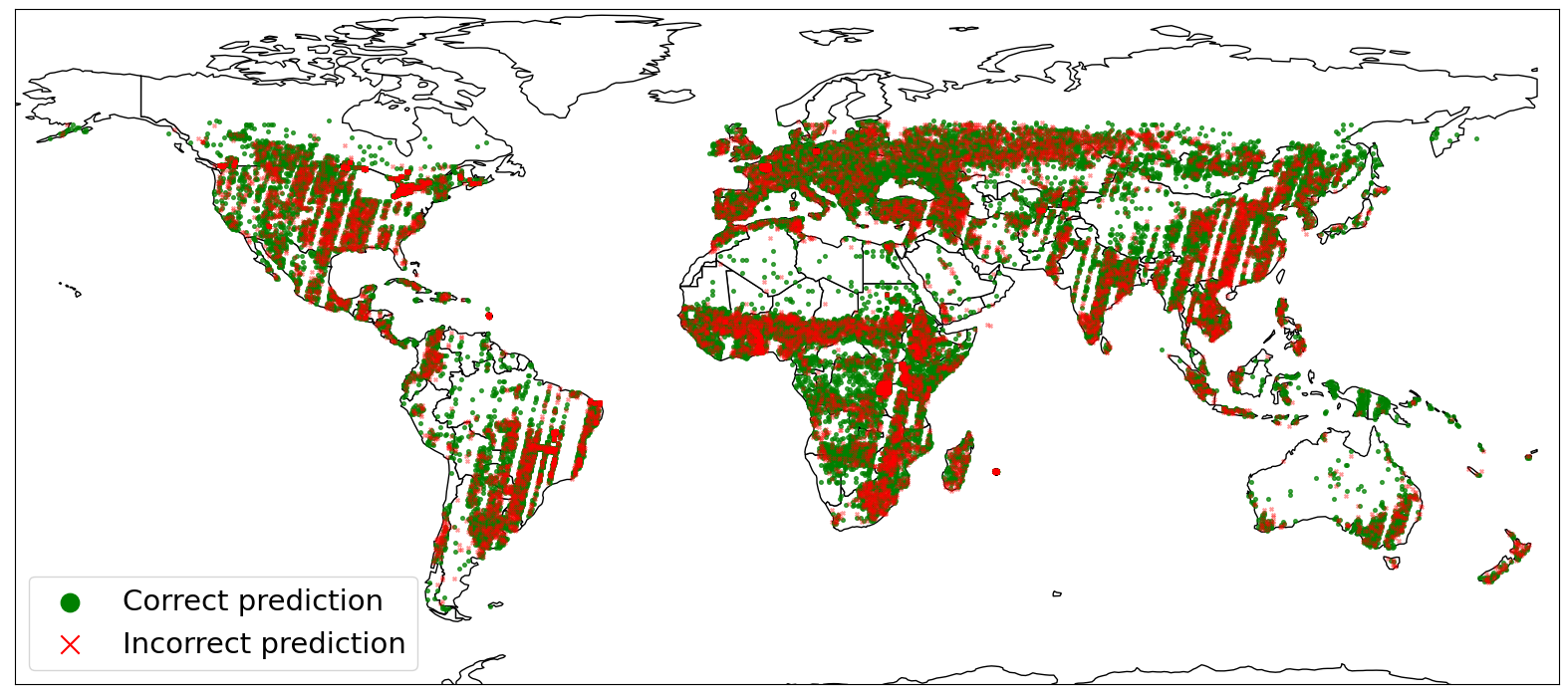
(a) Single-view model fed with the optical view.

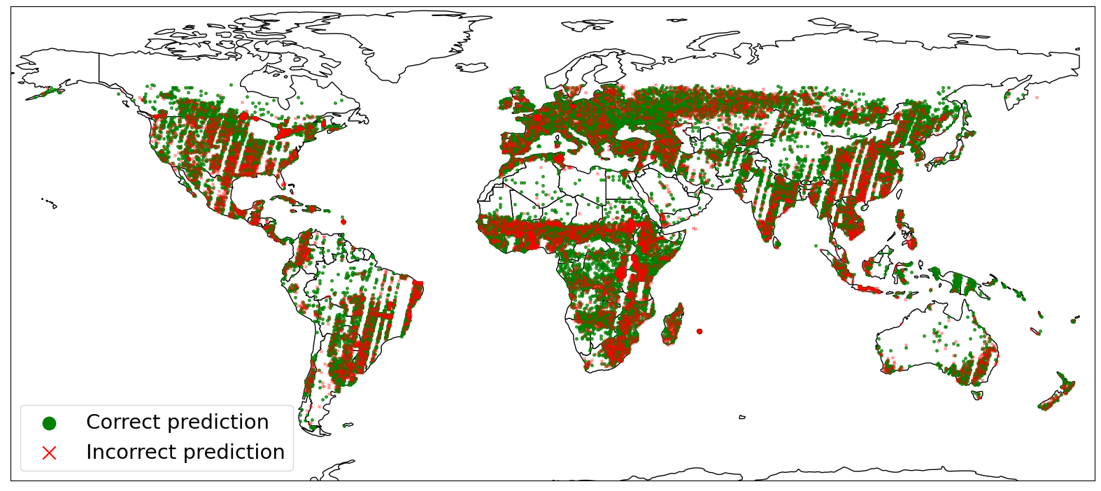
(b) MVL model with Input strategy.

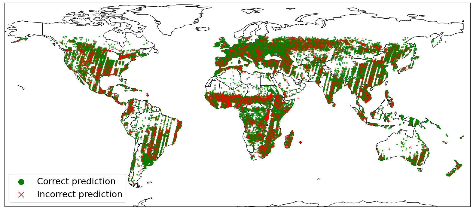
(c) MVL model with Decision strategy.

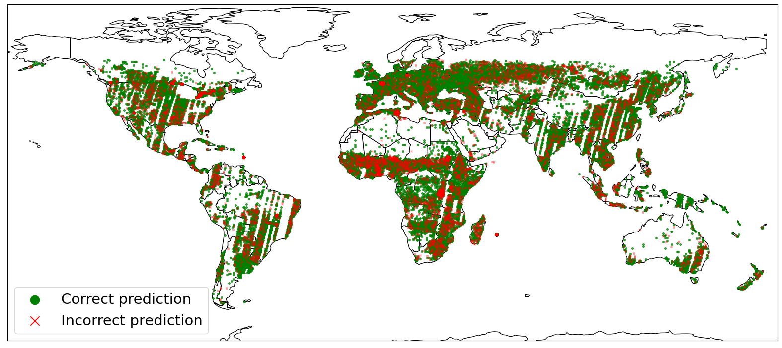
(d) MVL model with Hybrid gated strategy.

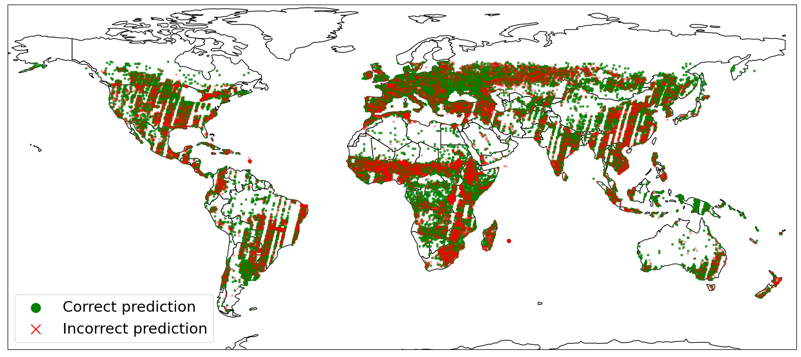
(e) MVL model with Ensemble strategy.

Figure A1: Predicted data points in the Global Binary evaluation for different fusion strategies using TempCNN as encoder. Red crosses are points with the predicted class equals to the target class, while green circles are samples with the predicted class different from the target.

(a) Single-view model fed with the optical view.

(b) MVL model with Input strategy.

(c) MVL model with Decision strategy.

(d) MVL model with Hybrid gated strategy.

(e) MVL model with Ensemble strategy.

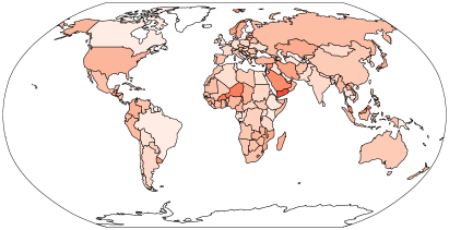
(f) MVL model with Feature gated strategy.

Figure A2: Error heatmap in the Global Binary evaluation for different fusion strategies using TempCNN as encoder. A stronger red color means more errors in specific countries.

References

- [Audebert et al., 2018] Audebert, N., Le Saux, B., and Lefèvre, S. (2018). Beyond RGB: Very high resolution urban remote sensing with multimodal deep networks. ISPRS Journal of Photogrammetry and Remote Sensing, 140:20–32.
- [Benedetti et al., 2018] Benedetti, P., Ienco, D., Gaetano, R., Ose, K., Pensa, R., and Dupuy, S. (2018). M3Fusion: A deep learning architecture for multiscale multimodal multitemporal satellite data fusion. IEEE J. Sel. Top. Appl. Earth Obs. Remote Sens., 11(12):4939–4949.
- [Camps-Valls et al., 2021] Camps-Valls, G., Tuia, D., Zhu, X. X., and Reichstein, M. (2021). Deep learning for the Earth Sciences: A comprehensive approach to remote sensing, climate science and geosciences. John Wiley & Sons.
- [Cho et al., 2014] Cho, K., van Merriënboer, B., Bahdanau, D., and Bengio, Y. (2014). On the properties of neural machine translation: Encoder–decoder approaches. In 8th Workshop on Syntax, Semantics and Structure in Statistical Translation, SSST 2014, pages 103–111. Association for Computational Linguistics (ACL).
- [Cué La Rosa et al., 2018] Cué La Rosa, L. E., Happ, P. N., and Feitosa, R. Q. (2018). Dense fully convolutional networks for crop recognition from multitemporal SAR image sequences. In IEEE International Geoscience and Remote Sensing Symposium (IGARSS), pages 7460–7463.
- [Dobrinić et al., 2021] Dobrinić, D., Gašparović, M., and Medak, D. (2021). Sentinel-1 and 2 time-series for vegetation mapping using random forest classification: A case study of Northern Croatia. Remote Sensing, 13(12):2321.
- [Ferrari et al., 2023] Ferrari, F., Ferreira, M. P., Almeida, C. A., and Feitosa, R. Q. (2023). Fusing Sentinel-1 and Sentinel-2 images for deforestation detection in the Brazilian Amazon under diverse cloud conditions. IEEE Geoscience and Remote Sensing Letters, 20:1–5.
- [Gadiraju et al., 2020] Gadiraju, K. K., Ramachandra, B., Chen, Z., and Vatsavai, R. R. (2020). Multimodal deep learning based crop classification using multispectral and multitemporal satellite imagery. In Proceedings of the International Conference on Knowledge Discovery & Data Mining (SIGKDD), pages 3234–3242. ACM.
- [Garnot and Landrieu, 2020] Garnot, V. S. F. and Landrieu, L. (2020). Lightweight temporal self-attention for classifying satellite images time series. In Advanced Analytics and Learning on Temporal Data: 5th ECML PKDD Workshop, pages 171–181. Springer.
- [Garnot et al., 2019] Garnot, V. S. F., Landrieu, L., Giordano, S., and Chehata, N. (2019). Time-space tradeoff in deep learning models for crop classification on satellite multi-spectral image time series. In IEEE International Geoscience and Remote Sensing Symposium (IGARSS), pages 6247–6250. IEEE.
- [Garnot et al., 2020] Garnot, V. S. F., Landrieu, L., Giordano, S., and Chehata, N. (2020). Satellite image time series classification with pixel-set encoders and temporal self-attention. In Proceedings of the IEEE/CVF Conference on Computer Vision and Pattern Recognition, pages 12325–12334.
- [Hochreiter and Schmidhuber, 1997] Hochreiter, S. and Schmidhuber, J. (1997). Long short-term memory. Neural computation, 9(8):1735–1780.
- [Hong et al., 2021] Hong, D., Gao, L., Yokoya, N., Yao, J., Chanussot, J., Du, Q., and Zhang, B. (2021). More diverse means better: Multimodal deep learning meets remote-sensing imagery classification. IEEE Transactions on Geoscience and Remote Sensing, 59(5):4340–4354.
- [Inglada et al., 2016] Inglada, J., Vincent, A., Arias, M., and Marais-Sicre, C. (2016). Improved early crop type identification by joint use of high temporal resolution SAR and optical image time series. Remote Sensing, 8(5):362.
- [Inouye et al., 1991] Inouye, T., Shinosaki, K., Sakamoto, H., Toi, S., Ukai, S., Iyama, A., Katsuda, Y., and Hirano, M. (1991). Quantification of EEG irregularity by use of the entropy of the power spectrum. Electroencephalography and clinical neurophysiology, 79(3):204–210.
- [Kang et al., 2020] Kang, Y., Ozdogan, M., Zhu, X., Ye, Z., Hain, C., and Anderson, M. (2020). Comparative assessment of environmental variables and machine learning algorithms for maize yield prediction in the US Midwest. Environmental Research Letters, 15(6):064005.
- [King and Zeng, 2001] King, G. and Zeng, L. (2001). Logistic regression in rare events data. Political analysis, 9(2):137–163.
- [Liu and Abd-Elrahman, 2018] Liu, T. and Abd-Elrahman, A. (2018). Deep convolutional neural network training enrichment using multi-view object-based analysis of Unmanned Aerial systems imagery for wetlands classification. ISPRS Journal of Photogrammetry and Remote Sensing, 139:154–170.
- [M Rustowicz et al., 2019] M Rustowicz, R., Cheong, R., Wang, L., Ermon, S., Burke, M., and Lobell, D. (2019). Semantic segmentation of crop type in Africa: A novel dataset and analysis of deep learning methods. In Proceedings of the IEEE/CVF Conference on Computer Vision and Pattern Recognition Workshops, pages 75–82.
- [Ma et al., 2022] Ma, M., Ren, J., Zhao, L., Testuggine, D., and Peng, X. (2022). Are multimodal transformers robust to missing modality? In Proceedings of the IEEE/CVF Conference on Computer Vision and Pattern Recognition, pages 18177–18186.
- [Malinin and Gales, 2018] Malinin, A. and Gales, M. (2018). Predictive uncertainty estimation via prior networks. Advances in neural information processing systems, 31.
- [Masolele et al., 2021] Masolele, R. N., De Sy, V., Herold, M., Marcos, D., Verbesselt, J., Gieseke, F., Mullissa, A. G., and Martius, C. (2021). Spatial and temporal deep learning methods for deriving land-use following deforestation: A pan-tropical case study using Landsat time series. Remote Sensing of Environment, 264:112600.
- [Masoudnia and Ebrahimpour, 2014] Masoudnia, S. and Ebrahimpour, R. (2014). Mixture of experts: A literature survey. Artificial Intelligence Review, 42:275–293.
- [Mena et al., 2023] Mena, F., Arenas, D., Nuske, M., and Dengel, A. (2023). A comparative assessment of multi-view fusion learning for crop classification. In IGARSS 2023 - IEEE International Geoscience and Remote Sensing Symposium, pages 5631–5634.
- [Mena et al., 2024a] Mena, F., Arenas, D., Nuske, M., and Dengel, A. (2024a). Common practices and taxonomy in deep multi-view fusion for remote sensing applications. IEEE Journal of Selected Topics in Applied Earth Observations and Remote Sensing.
- [Mena et al., 2024b] Mena, F., Pathak, D., Najjar, H., Sanchez, C., Helber, P., Bischke, B., Habelitz, P., Miranda, M., Siddamsetty, J., Nuske, M., et al. (2024b). Adaptive fusion of multi-view remote sensing data for optimal sub-field crop yield prediction. arXiv preprint arXiv:2401.11844.
- [Ofori-Ampofo et al., 2021] Ofori-Ampofo, S., Pelletier, C., and Lang, S. (2021). Crop type mapping from optical and radar time series using attention-based deep learning. Remote Sensing, 13(22).
- [Pathak et al., 2023] Pathak, D., Miranda, M., Mena, F., Sanchez, C., Helber, P., Bischke, B., Habelitz, P., Najjar, H., Siddamsetty, J., Arenas, D., et al. (2023). Predicting crop yield with machine learning: An extensive analysis of input modalities and models on a field and sub-field level. In IGARSS 2023-2023 IEEE International Geoscience and Remote Sensing Symposium, pages 2767–2770. IEEE.
- [Pelletier et al., 2019] Pelletier, C., Webb, G. I., and Petitjean, F. (2019). Temporal convolutional neural network for the classification of satellite image time series. Remote Sensing, 11(5):523.
- [Rußwurm and Korner, 2017] Rußwurm, M. and Korner, M. (2017). Temporal vegetation modelling using long short-term memory networks for crop identification from medium-resolution multi-spectral satellite images. In Proceedings of the IEEE/CVF Conference on Computer Vision and Pattern Recognition Workshops, pages 11–19.
- [Rußwurm and Körner, 2020] Rußwurm, M. and Körner, M. (2020). Self-attention for raw optical satellite time series classification. ISPRS journal of photogrammetry and remote sensing, 169:421–435.
- [Sainte Fare Garnot et al., 2022] Sainte Fare Garnot, V., Landrieu, L., and Chehata, N. (2022). Multi-modal temporal attention models for crop mapping from satellite time series. ISPRS Journal of Photogrammetry and Remote Sensing, 187:294–305.
- [Schneider et al., 2023] Schneider, M., Schelte, T., Schmitz, F., and Körner, M. (2023). EuroCrops: The largest harmonized open crop dataset across the European Union. Scientific Data, 10(1):612.
- [Sheng et al., 2020] Sheng, H., Chen, X., Su, J., Rajagopal, R., and Ng, A. (2020). Effective data fusion with generalized vegetation index: Evidence from land cover segmentation in agriculture. In Proceedings of the IEEE/CVF conference on computer vision and pattern recognition workshops, pages 60–61.
- [Torbick et al., 2018] Torbick, N., Huang, X., Ziniti, B., Johnson, D., Masek, J., and Reba, M. (2018). Fusion of moderate resolution earth observations for operational crop type mapping. Remote Sensing, 10(7):1058.
- [Tseng et al., 2022] Tseng, G., Kerner, H., and Rolnick, D. (2022). TIML: Task-informed meta-learning for agriculture. arXiv preprint arXiv:2202.02124.
- [Tseng et al., 2021] Tseng, G., Zvonkov, I., Nakalembe, C. L., and Kerner, H. (2021). CropHarvest: A global dataset for crop-type classification. Proceedings of NIPS Datasets and Benchmarks Track.
- [Tseng et al., 2023] Tseng, G., Zvonkov, I., Purohit, M., Rolnick, D., and Kerner, H. (2023). Lightweight, pre-trained transformers for remote sensing timeseries. arXiv preprint arXiv:2304.14065.
- [Van der Maaten and Hinton, 2008] Van der Maaten, L. and Hinton, G. (2008). Visualizing data using t-SNE. Journal of machine learning research, 9(11).
- [Vaswani et al., 2017] Vaswani, A., Shazeer, N., Parmar, N., Uszkoreit, J., Jones, L., Gomez, A. N., Kaiser, Ł., and Polosukhin, I. (2017). Attention is all you need. Advances in neural information processing systems, 30.
- [Weilandt et al., 2023] Weilandt, F., Behling, R., Goncalves, R., Madadi, A., Richter, L., Sanona, T., Spengler, D., and Welsch, J. (2023). Early crop classification via multi-modal satellite data fusion and temporal attention. Remote Sensing, 15(3).
- [Yan et al., 2021] Yan, X., Hu, S., Mao, Y., Ye, Y., and Yu, H. (2021). Deep multi-view learning methods: A review. Neurocomputing, 448:106–129.
- [Yuan et al., 2022] Yuan, Y., Lin, L., Liu, Q., Hang, R., and Zhou, Z.-G. (2022). SITS-Former: A pre-trained spatio-spectral-temporal representation model for Sentinel-2 time series classification. International Journal of Applied Earth Observation and Geoinformation, 106:102651.
- [Zhang et al., 2020] Zhang, P., Du, P., Lin, C., Wang, X., Li, E., Xue, Z., and Bai, X. (2020). A hybrid attention-aware fusion network (HAFNet) for building extraction from high-resolution imagery and LiDAR data. Remote Sensing, 12(22).
- [Zhao et al., 2021] Zhao, H., Duan, S., Liu, J., Sun, L., and Reymondin, L. (2021). Evaluation of five deep learning models for crop type mapping using Sentinel-2 time series images with missing information. Remote Sensing, 13(14):2790.
- [Zhong et al., 2019] Zhong, L., Hu, L., and Zhou, H. (2019). Deep learning based multi-temporal crop classification. Remote sensing of environment, 221:430–443.