Decoupling parameter variation from noise:
Biquadratic Lyapunov forms in data-driven LPV control

Abstract

A promising step from linear towards nonlinear data-driven control is via the design of controllers for linear parameter-varying (LPV) systems, which are linear systems whose parameters are varying along a measurable scheduling signal. However, the interplay between uncertainty arising from corrupted data and the parameter-varying nature of these systems impacts the stability analysis, and limits the generalization of well-understood data-driven methods for linear time-invariant systems. In this work, we decouple this interplay using a recently developed variant of the Fundamental Lemma for LPV systems and the viewpoint of data-informativity, in combination with biquadratic Lyapunov forms. Together, these allow us to develop novel linear matrix inequality conditions for the existence of scheduling-dependent Lyapunov functions, incorporating the intrinsic nonlinearity. Appealingly, these results are stated purely in terms of the collected data and bounds on the noise, and they are computationally favorable to check.

I Introduction

Linear and model-based controller design, i.e., controller design based on a known linear model of the system, is widespread in both theoretical and practical applications. However, engineering systems are becoming more complex with demanding requirements in terms of performance, interconnectivity and energy efficiency. Hence, handling unknown and nonlinear behaviors is utterly important. For such systems having access to ‘a known model of the system’ can be costly and requires expertise. The wish for (automated) model-free design with hard theoretical guarantees sparked interest in the field of direct data-driven control, where the controller is designed directly based on measured data. Lately, a paradigm in which the measurements themselves are viewed as a representation of the system behavior has been gaining a lot of attention (see, e.g., [1]). This avoids the need for an identification step and thus a model (see [2] for a discussion on when to use models). Important concepts within this paradigm are, e.g., Willems’ Fundamental Lemma [3], data informativity [4, 5] and identifiability [6]. However, these have been mainly focusing on linear time-invariant (LTI) systems, apart for some extensions for specific classes of nonlinear systems [7, 8, 9, 10, 11, 12]. In this paper, we will show that these ideas can also be applied to linear parameter-varying (LPV) systems, which are often used as surrogates of nonlinear systems. See, e.g., [13, 14] for alternative data-driven LPV control methods.

The LPV framework considers systems where a linear input-(state)-output relationship is varying along a so-called scheduling signal. This signal is used to capture time-varying and/or nonlinear aspects of the system behavior. Assuming that the scheduling signal is measurable and varying within a bounded set, the LPV framework has proven capable of systematically handling a range of complex nonlinear control problems whilst retaining many of the desirable properties of LTI control, see [15, 16] and references therein. The fact that this approach can be used in nonlinear data-driven control has been (experimentally) shown in [17, 18] using the LPV extension of Willems’ Fundamental Lemma [19]. These works, however, do not consider noise corrupted data. We aim to overcome this by employing ideas from the data-informativity framework. In simple terms, this means that we characterize the set of all LPV systems that could have generated the observed data-set with bounded disturbances. This set is then used to find a Lyapunov function and a controller that guarantee (robust) stability against any uncertainty introduced by both the noise and the scheduling variation. The combination of data-informativity and the LPV framework has been considered before [20]. However, the results of [20] guarantee stability with a single, robust (i.e., scheduling-independent) Lyapunov function. This means that this single Lyapunov function is required to decrease, i.e., prove stability of the closed-loop LPV system, for all possible variations of the scheduling and assumed noise realizations. This can introduce significant conservatism in the stability analysis, and hence in the data-driven controller design. In this work, we decouple the interplay between the uncertainty introduced due to noise in the data and parameter variation along the scheduling signal within the LPV data-informativity framework. We do so by considering Lyapunov functions that are biquadratic forms, that is, quadratic in both the state and scheduling signals.

This work contains the following contributions:

1. We derive conditions for stability analysis using biquadratic Lyapunov functions for discrete-time LPV systems. In particular, these generalize previously known results.

2. We use the conditions of C1 to formulate LPV control design methods within the informativity framework for LPV systems. This yields linear matrix inequality (LMI) based conditions that can be efficiently solved in a semi-definite program (SDP).

3. We demonstrate the increased stability and robustness range resulting from our methods using a nonlinear simulation example.

The remainder of the paper is structured as follows: Section II provides the system class and the formal problem statement. Section III and IV discuss QMIs and LPV stability analysis with biquadratic Lyapunov functions, respectively, which we use in the formulation of our data-driven synthesis results in Section V. We demonstrate the advantages of our method in Section VI and give the conclusions in Section VII.

Notation

The identity matrix is denoted by $I_{n}\in\mathbb{R}^{n\times n}$, while $1_{n}$ denotes the vector $\begin{bmatrix}1&\cdots&1\end{bmatrix}^{\top}\in\mathbb{R}^{n}$. The set of real symmetric matrices of size $n\times n$ is denoted by $\mathbb{S}^{n}$. $X\succ 0$ and $X\prec 0$ ($X\succeq 0$ and $X\preceq 0$) stands for positive/negative (semi) definiteness of a symmetric matrix $X\in\mathbb{S}^{n}$, respectively. The Kronecker product of $A\in\mathbb{R}^{n\times m}$ and $B\in\mathbb{R}^{p\times q}$ is denoted by $A\otimes B\in\mathbb{R}^{pm\times qn}$. Block diagonal concatenation of matrices is given by $\mathrm{blkdiag}$. For $X=\begin{bmatrix}A&B\\ B^{\top}&C\end{bmatrix}$, $X\mid A$ is a shorthand taking the Schur complement of $X$ w.r.t. $A$, i.e., $X\mid A=C-B^{\top}A^{-1}B$.

II Preliminaries

II-A System definition

Consider a discrete-time data-generating LPV system with full state-observation that can be represented by

$$x_{k+1}=A(p_{k})x_{k}+Bu_{k}+w_{k},$$ (1)

where $k\in\mathbb{Z}$ is the discrete time, $x_{k}\in\mathbb{R}^{n_{\mathrm{x}}}$, $u_{k}\in\mathbb{R}^{n_{\mathrm{u}}}$ and $p_{k}\in\mathbb{P}\subset\mathbb{R}^{n_{\mathrm{p}}}$ are the measurable state, input and scheduling signals, respectively, and $\mathbb{P}$ is a compact, convex set that defines the range of the scheduling signal. By the nature of the LPV framework, the signal $p_{k}$ is considered to be accessible to us, and can be either exogenous or endogenous, i.e., independent from $x,u,w$, or composed as, e.g., $p_{k}:=\psi(x_{k})$ for some function $\psi$. The LPV system is disturbed by a $w_{k}\in\mathbb{R}^{n_{\mathrm{x}}}$, which can act as a process disturbance or a (colored) noise process. Note that $B$ here is taken constant due to technical convenience and can easily be overcome by state-augmentation or propagating $u$ through an LTI filter. The matrix function $A:\mathbb{P}\rightarrow\mathbb{R}^{n_{\mathrm{x}}\times n_{\mathrm{x}}}$ is considered to have affine dependency on $p_{k}$, which is a common assumption in practice, cf. [15, 21],

$$A(p_{k})=A_{0}+{\textstyle\sum_{i=1}^{n_{\mathrm{p}}}}p_{i,k}A_{i},$$ (2)

where $A_{i}\in\mathbb{R}^{n_{\mathrm{x}}\times n_{\mathrm{x}}}$. The affine scheduling dependence of $A(p_{k})$ allows us to write the data-generating system (1) as

$$x_{k+1}=\mathcal{A}L_{p_{k}}x_{k}+Bu_{k}+w_{k},$$ (3)

where we define the shorthand

$$\mathcal{A}:=\begin{bmatrix}A_{0}&A_{1}&\cdots&A_{n_{\mathrm{p}}}\end{bmatrix},\quad L_{p_{k}}:=\begin{bmatrix}1\\ p_{k}\end{bmatrix}\otimes I_{n_{\mathrm{x}}}.$$ (4)

Apart from the structure (2), we assume that (1) is unknown. Instead, we have access to measurements of $x,u$ and $p$, where $x$ is a sample path realization with respect to $u,p,$ and the disturbance $w$. Note that this means that for endogenous $p$, the map $\psi$ is known. The measurements are collected in

$$\Phi :=\begin{bmatrix}L_{p_{0}}x_{0}&\cdots&L_{p_{{N_{\mathrm{d}}}-1}}x_{{N_{\mathrm{d}}}-1}\\ u_{0}&\cdots&u_{{N_{\mathrm{d}}}-1}\end{bmatrix},$$ (5a)

$$X_{+} :=\begin{bmatrix}x_{1}&\cdots&x_{N_{\mathrm{d}}}\end{bmatrix},$$ (5b)

where $L_{p_{k}}x_{k}=\begin{bmatrix}x_{k}^{\top}\!&\!(p_{k}\otimes x_{k})^{\top}\end{bmatrix}_{{}^{{}^{\text{\normalsize,}}}}^{\top}$ and corresponding

$$W_{-}:=\begin{bmatrix}w_{0}&\cdots&w_{{N_{\mathrm{d}}}-1}\end{bmatrix}.$$ (6)

The amount of information regarding the system dynamics that is encoded in the data can be quantified by the rank of $\Phi$. In particular, if $\Phi$ has full row-rank, i.e., $\mathrm{rank}(\Phi)=n_{\mathrm{u}}+n_{\mathrm{x}}(1+n_{\mathrm{p}})$, it is said that the data is persistently exciting (PE) [22].

II-B Problem statement

Given the above, we are interested in data-based LPV controller synthesis for systems of the form (3) using only measurements of $x,p$ and $u$. More specifically, we aim at designing a stabilizing LPV state-feedback controller for (3) using only the measured data-set (5), a boundedness assumption on the noise signal (6), and the range for $p$, i.e., $\mathbb{P}\subset\mathbb{R}^{n_{\mathrm{p}}}$. In particular, we will take the viewpoint of the informativity framework, meaning that we observe that a controller is guaranteed to stabilize the true system only if it stabilizes all systems compatible with (5).

In order to develop computationally tractable tests, we will make the following technical assumptions:

1. The data-generating system (1) admits a realization of the form (3).

2. The measured data is PE, i.e., $\Phi$ in (5) is full row-rank.

3. The noise matrix $W_{-}$ is bounded in terms of a quadratic matrix inequality (QMI).

We will discuss the technicalities of these assumptions the sections that follow.

III Quadratic matrix inequalities in control

III-A Disturbance model

We assume that the disturbances are compatible with a QMI in terms of a finite-time trajectory, compatible with (5). This means that, for some $\Pi\in\mathbb{S}^{n_{\mathrm{x}}+{N_{\mathrm{d}}}}$,

$$\begin{bmatrix}I_{n_{\mathrm{x}}}\\ W_{-}^{\top}\end{bmatrix}^{\top}\Pi\begin{bmatrix}I_{n_{\mathrm{x}}}\\ W_{-}^{\top}\end{bmatrix}\succcurlyeq 0.$$ (7)

The feasible sets of such QMIs will play a major role in this work. Hence, we define for some $\Psi\in\mathbb{S}^{q+r}$ sets of the form

$$\mathcal{Z}_{\mathrm{r}}(\Psi):=\left\{\vphantom{\begin{bmatrix}I_{q}\\ Z\end{bmatrix}^{\top}\Psi\begin{bmatrix}I_{q}\\ Z\end{bmatrix}\succcurlyeq 0}Z\in\mathbb{R}^{r\times q}\right.\left|\,\vphantom{Z\in\mathbb{R}^{r\times q}}\begin{bmatrix}I_{q}\\ Z\end{bmatrix}^{\top}\Psi\begin{bmatrix}I_{q}\\ Z\end{bmatrix}\succcurlyeq 0\right\}.$$ (8a)

Similarly, the interior of (8a) is defined by the strict variant:

$$\mathcal{Z}^{+}_{\mathrm{r}}(\Psi):=\left\{\vphantom{\begin{bmatrix}I_{q}\\ Z\end{bmatrix}^{\top}\Psi\begin{bmatrix}I_{q}\\ Z\end{bmatrix}\succ 0}Z\in\mathbb{R}^{r\times q}\right.\left|\,\vphantom{Z\in\mathbb{R}^{r\times q}}\begin{bmatrix}I_{q}\\ Z\end{bmatrix}^{\top}\Psi\begin{bmatrix}I_{q}\\ Z\end{bmatrix}\succ 0\right\}.$$ (8b)

On the basis of these definitions in (7), (8), we have that

$$W_{-}^{\top}\in\mathcal{Z}_{n_{\mathrm{x}}}(\Pi).$$ (9)

Remark 1 (On the noise model).

For the existence of disturbances $w$, i.e., $\mathcal{Z}_{n_{\mathrm{x}}}(\Pi)\neq\varnothing$, we require $\Pi\mid\Pi_{22}\succcurlyeq 0$. Furthermore, to guarantee bounded disturbances, we require $\Pi_{22}\prec 0$. A simple example satisfying both is $\Pi=\mathrm{blkdiag}(\Omega,-I_{{N_{\mathrm{d}}}})$ with $\Omega\succcurlyeq 0$. This means that

$$W_{-}W_{-}^{\top}={\textstyle\sum_{k=0}^{{N_{\mathrm{d}}}-1}}w_{k}w_{k}^{\top}\preccurlyeq\Omega,$$ (10)

that is, we have an energy bound on $W_{-}$ defined by $\Omega$. In [23, Sec. 2] other properties of such noise models are discussed. In particular, confidence regions of (colored) Gaussian noise fall into this category [23, Sec. 5.4].

III-B Set of LPV systems compatible with  (5)

Note that $\mathcal{A},B$ parametrize an LPV system of the form (3) and that $n_{\mathrm{x}},n_{\mathrm{u}}$ and $n_{\mathrm{p}}$ follow directly from (5). Hence, in line with the informativity framework, we can then define the set of LPV systems that are compatible with the measurements (5) under the disturbance model (7):

$$X_{+}=\begin{bmatrix}\mathcal{A}&B\end{bmatrix}\Phi+W_{-},\quad W_{-}^{\top}\in\mathcal{Z}_{n_{\mathrm{x}}}(\Pi).$$

Hence, all possible $\mathcal{A},B$ that could have generated the data-set in (5) are characterized by the QMI

$$\begin{bmatrix}I\\ \mathcal{A}^{\top}\\ B^{\top}\end{bmatrix}^{\top}\underbrace{\begin{bmatrix}I&X_{+}\\ 0&-\Phi\end{bmatrix}\Pi\begin{bmatrix}I&X_{+}\\ 0&-\Phi\end{bmatrix}^{\top}}_{=:N}\begin{bmatrix}I\\ \mathcal{A}^{\top}\\ B^{\top}\end{bmatrix}\succcurlyeq 0,$$ (11)

where $N\in\mathbb{S}^{n_{\mathrm{u}}+n_{\mathrm{x}}(2+n_{\mathrm{p}})}$. In shorthand, we can write $\begin{bmatrix}\mathcal{A}&B\end{bmatrix}^{\top}\in\mathcal{Z}_{n_{\mathrm{u}}+n_{\mathrm{x}}(1+n_{\mathrm{p}})}(N)$. In this paper, we will assume that the true realization of the noise signal satisfies the noise bound. This means that this set is nonempty by default. Clearly, a having a conservative noise bound will lead to larger sets of systems, impeding controller design.

IV Stability analysis of LPV systems

IV-A Controller structure

To stabilize the system (1), we will design an LPV state-feedback controller. The state and scheduling signals are measurable and thus available for control, and hence, we design a controller

$$u_{k}=K(x_{k},p_{k}),$$ (12a)

where we choose $$K:\mathbb{R}^{n_{\mathrm{x}}}\times\mathbb{R}^{n_{\mathrm{p}}}\to\mathbb{R}^{n_{\mathrm{u}}} p_{k} x_{k}$$ to have affine dependence on and linear dependence on :

$$K(x_{k},p_{k})=\left(K_{0}+\sum_{i=1}^{n_{\mathrm{p}}}p_{i,k}K_{i}\right)x_{k}=\mathcal{K}L_{p_{k}}x_{k},$$ (12b)

with $$\mathcal{K}:=\begin{bmatrix}K_{0}&K_{1}&\cdots&K_{n_{\mathrm{p}}}\end{bmatrix}$$.

This allows us to write the closed-loop system as

$$x_{k+1}=(\mathcal{A}+B\mathcal{K})\begin{bmatrix}x_{k}\\ p_{k}\otimes x_{k}\end{bmatrix}+w_{k}\\ =(\mathcal{A}+B\mathcal{K})L_{p_{k}}x_{k}+w_{k}.$$ (13)

Hence, the closed-loop is of the same system class as (1). There are a plethora of model-based synthesis methods available for this class of LPV systems. However, in terms of fully data-driven LPV controller synthesis approaches, only [22] (considering only noise-free data) and [20] (using common Lyapunov functions) are available. We aim to use biquadratic Lyapunov functions, making the analysis (and later synthesis) problem both tractable and less conservative.

IV-B Biquadratic Lyapunov functions

Let for the remainder of this section $w_{k}\equiv 0$. In order to guarantee asymptotic stability of LPV systems of the form (13) under arbitrary variation of $p_{k}\in\mathbb{P}$, we aim at finding a scheduling-dependent Lyapunov function that ensures that the LPV system is stable. Hence, we are looking for a $V:\mathbb{R}^{n_{\mathrm{x}}}\times\mathbb{P}\mapsto\mathbb{R}_{\geq 0}$ that satisfies

$$\alpha(\|x\|)\leq V(x,p)\leq\beta(\|x\|),$$ (14)

where $\alpha,\beta$ are class-$K$ functions, and

$$V(x_{k+1},p_{k+1})<V(x_{k},p_{k}),$$ (15)

for all scheduling sequences $p_{k},p_{k+1}\in\mathbb{P}$ and states $x_{k},x_{k+1}\in\mathbb{R}^{n_{\mathrm{x}}}\setminus\{0\}$ satisfying (13). We want to highlight that if (1) is an embedding of a nonlinear system, i.e., $p_{k}:=\psi(x_{k})$, then asymptotic stability of (1) implies asymptotic stability of the origin of the corresponding nonlinear system [24].

As the above class of Lyapunov functions is rather general, the tractability of such Lyapunov stability analysis is limited. The usual method of enabling computationally efficient conditions is to assume that the Lyapunov function does not depend on $p$ and is just a quadratic form in $x$, as for LTI systems. Instead, here we consider a class of biquadratic Lyapunov functions. Thus, we choose $V(x,p)$ to have quadratic dependence on both $x$ and $p$. Without loss of generality,

$$V(x_{k},p_{k})=x_{k}^{\top}L_{p_{k}}^{\top}PL_{p_{k}}x_{k}.$$ (16)

where $P\in\mathbb{S}^{n_{\mathrm{x}}(n_{\mathrm{p}}+1)}$, and $L_{p_{k}}$ is as defined in (4). In order to guarantee (14), we take $P\succ 0$.

Remark 2 (On positive definiteness and SOS).

Note that (14) does not only hold if $P\succ 0$. As such, this assumption introduces some conservativeness. One could employ sum-of-squares techniques to test whether for a given $P$ the function $V(x,p)$ is positive definite instead. This reduces this gap at the cost of an increase in computational complexity. However, sum-of-squares is only nonconservative for the case where either $n_{\mathrm{x}}=2$ or $n_{\mathrm{p}}=1$ (see e.g. [25]).

Remark 3 (On biquadratic Lyapunov functions).

The specific quadratic scheduling-dependence introduced for the Lyapunov functions, i.e., (16), has been introduced for continuous-time LPV systems in [26], where they are used to find controllers with better performance. To the best of our knowledge, the extension towards discrete-time LPV systems has so far not been made.

Since we will prove asymptotic stability using the existence of such a biquadratic Lyapunov function, we can derive the following sufficient condition for stability.

Lemma 1.

Given an LPV system (13), and $V(x_{k},p_{k})=x_{k}^{\top}L_{p_{k}}^{\top}PL_{p_{k}}x_{k}$, where $P\succ 0$. Then

$$V(x_{k+1},p_{k+1})<V(x_{k},p_{k}),$$

for all $x_{k},x_{k+1}\in\mathbb{R}^{n_{\mathrm{x}}}\setminus\{0\}$ and $p_{k},p_{k+1}\in\mathbb{P}$ satisfying the dynamics (13), if for all $p_{k+1}\in\mathbb{P}$

$$P^{-1}-L_{p_{k+1}}(\mathcal{A}+B\mathcal{K})P^{-1}(\mathcal{A}+B\mathcal{K})^{\top}L_{p_{k+1}}^{\top}\succ 0.$$ (17)

Proof.

Since $P\succ 0$, we can employ the Schur complement to show that (17) is equivalent to

$$\begin{bmatrix}P^{-1}&L_{p_{k+1}}(\mathcal{A}+B\mathcal{K})\\ (\mathcal{A}+B\mathcal{K})^{\top}L_{p_{k+1}}^{\top}&P\end{bmatrix}\succ 0.$$

Repeating the argument with respect to the other block, we have equivalently:

$$P-(\mathcal{A}+B\mathcal{K})^{\top}L_{p_{k+1}}^{\top}PL_{p_{k+1}}(\mathcal{A}+B\mathcal{K})\succ 0.$$ (18)

Let $x_{k}\neq 0$ and $p_{k}\in\mathbb{P}$, then we have that $x_{k}^{\top}L_{p_{k}}^{\top}\neq 0$. Therefore, by premultiplying the last inequality with $x_{k}^{\top}L_{p_{k}}^{\top}$ and postmultiplying with its transpose we obtain:

$$\underbrace{x_{k}^{\top}L_{p_{k}}^{\top}PL_{p_{k}}x_{k}}_{V(x_{k},p_{k})}-\underbrace{x_{k+1}^{\top}L_{p_{k+1}}^{\top}PL_{p_{k+1}}x_{k+1}}_{V(x_{k+1},p_{k+1})}>0.$$ (19)

We can now conclude the lemma. ∎

Note that condition (17) is only sufficient for asymptotic stability. What inhibits this result from being necessary is the last step of the proof, where we derive (19) from (18). Analogous to the discussion in Remark 2, the former can hold under weaker conditions than positive definiteness of (18).

We now provided tools to analyze asymptotic stability of an LPV system with biquadratic Lyapunov functions under $w_{k}\equiv 0$. In the next section, we will integrate these tools in the data-informativity framework to formulate LPV controller synthesis conditions that are only dependent on the noisy data-set (5).

V Data-driven LPV controller synthesis

Apart from the assumptions presented in Section II-B, we require the technical condition in Remark 1 to hold:

Assumption 1.

$\Pi$ satisfies $\Pi\mid\Pi_{22}\succcurlyeq 0$ and $\Pi_{22}\prec 0$.

Note that these assumptions are simply conditions to be satisfied when designing the experiment. We are now ready to present our main results.

V-A Synthesis approach with scheduling-dependent S-Lemma

To recap our objective, we aim at finding $\mathcal{K}$ and $P\succ 0$ such that (17) holds for all scheduling variables $p_{k+1}\in\mathbb{P}$ and all systems $\mathcal{A},B$ for which $\begin{bmatrix}\mathcal{A}&B\end{bmatrix}^{\top}\in\mathcal{Z}_{n_{\mathrm{x}}(1+n_{\mathrm{p}})+n_{\mathrm{u}}}(N)$, i.e., satisfying (11).

In other words, we want that for every $Z$ and $p_{k+1}\in\mathbb{P}$:

$$\begin{bmatrix}I_{n_{\mathrm{x}}}\\ Z\end{bmatrix}^{\!\top}\!N\begin{bmatrix}I_{n_{\mathrm{x}}}\\ Z\end{bmatrix}\succcurlyeq 0\Rightarrow\begin{bmatrix}I_{n_{\mathrm{x}}(1+n_{\mathrm{p}})}\\ ZL_{p_{k+1}}^{\!\top}\end{bmatrix}^{\top}\!M\begin{bmatrix}I_{n_{\mathrm{x}}(1+n_{\mathrm{p}})}\\ ZL_{p_{k+1}}^{\top}\end{bmatrix}\succ 0,$$

where

$$M=\begin{bmatrix}P^{-1}&0\\ 0&-\begin{bmatrix}I_{n_{\mathrm{x}}(1+n_{\mathrm{p}})}\\ \mathcal{K}\end{bmatrix}P^{-1}\begin{bmatrix}I_{n_{\mathrm{x}}(1+n_{\mathrm{p}})}\\ \mathcal{K}\end{bmatrix}^{\top}\end{bmatrix}.$$

Even more concisely, we need:

$$(\mathcal{Z}_{n_{\mathrm{u}}+n_{\mathrm{x}}(1+n_{\mathrm{p}})}(N))L_{p_{k+1}}^{\top}\subseteq\mathcal{Z}_{n_{\mathrm{u}}+n_{\mathrm{x}}(1+n_{\mathrm{p}})}^{+}(M).$$ (20)

In simple terms, we require a linear transformation ($L_{p_{k+1}}^{\top}$) of the feasible region of a nonstrict QMI to be contained in the feasible region of a strict QMI. To reduce this to a simple QMI inclusion problem, we will employ [23, Thm 3.4]. For this, note that from Assumption 1, it follows that $N_{22}\prec 0$. This verifies the assumptions of the QMI result [23, Thm 3.4] and allows us to conclude:

Proposition 1.

Let Assumption 1 hold. Then, for any $p_{k}\in\mathbb{P}$

$$(\mathcal{Z}_{n_{\mathrm{u}}+n_{\mathrm{x}}(1+n_{\mathrm{p}})}(N))L_{p_{k}}^{\top}=\mathcal{Z}_{n_{\mathrm{u}}+n_{\mathrm{x}}(1+n_{\mathrm{p}})}(N_{p_{k}}),$$

where $N_{p_{k}}\in\mathbb{S}^{n_{\mathrm{u}}+2n_{\mathrm{x}}(1+n_{\mathrm{p}})}$ is defined as

$$N_{p_{k}}:= \begin{bmatrix}L_{p_{k}}&0\\ 0&I\end{bmatrix}N\begin{bmatrix}L_{p_{k}}^{\top}&0\\ 0&I\end{bmatrix}$$

$$= \begin{bmatrix}L_{p_{k}}&L_{p_{k}}X_{+}\\ 0&-\Phi\end{bmatrix}\Pi\begin{bmatrix}L_{p_{k}}&L_{p_{k}}X_{+}\\ 0&-\Phi\end{bmatrix}^{\top}.$$

Using this, (20) is equivalent to an inclusion between two feasible regions of QMI’s. We can now use the Matrix S-Lemma [23, Cor. 4.13] to resolve this to an LMI and conclude the following synthesis result.

Theorem 1.

Let Assumption 1 hold and fix a scheduling variable $p_{k+1}\in\mathbb{P}$. There exist scalars $\alpha\geq 0$ and $\beta>0$, a matrix $F\in\mathbb{S}^{n_{\mathrm{x}}(1+n_{\mathrm{p}})}$ such that $F\succ 0$, and a matrix $G\in\mathbb{R}^{n_{\mathrm{u}}\times n_{\mathrm{x}}(1+n_{\mathrm{p}})}$ such that

$$\begin{bmatrix}F-\beta I\!&0&0&0\\ 0&0&0&F\\ 0&0&0&G\\ 0&\!F&G^{\top}&F\end{bmatrix}-\alpha\begin{bmatrix}N_{p_{k+1}}\!\!&0\\ 0&0\end{bmatrix}\!\succcurlyeq 0,$$ (21)

if and only if inequality (17) holds with $\mathcal{K}=GF^{-1}$ and $P=F^{-1}$ for all systems $\begin{bmatrix}\mathcal{A}&B\end{bmatrix}^{\top}\in\mathcal{Z}_{n_{\mathrm{u}}+n_{\mathrm{x}}(1+n_{\mathrm{p}})}(N)$, that is, all systems consistent with the data.

Proof.

Starting from (20) we can apply Proposition 1 followed by the Matrix S-Lemma [23, Cor. 4.13]. The assumptions of the latter follow straightforwardly from Assumption 1. This yields that for a given $p_{k+1}\in\mathbb{P}$, we have (20) if and only if there exists $\alpha\geq 0$ and $\beta>0$ such that

$$M-\alpha N_{p_{k+1}}\succcurlyeq\begin{bmatrix}\beta I&0\\ 0&0\end{bmatrix}.$$

By a Schur complement argument, this, in turn, is equivalent to

$$\begin{bmatrix}P^{-1}-\beta I\!&0&0&0\\ 0&0&0&P^{-1}\\ 0&0&0&\mathcal{K}P^{-1}\\ 0&\!P^{-1}&P^{-1}\mathcal{K}^{\top}&P^{-1}\end{bmatrix}-\alpha\begin{bmatrix}N_{p_{k+1}}\!\!&0\\ 0&0\end{bmatrix}\!\succcurlyeq 0.$$

We can now perform the substitutions $\mathcal{K}=GF^{-1}$ and $P=F^{-1}$ to conclude the theorem. ∎

Theorem 1 provides a tractable condition, consisting of checking the feasibility of an LMI of size $3n_{\mathrm{x}}(1+n_{\mathrm{p}})+n_{\mathrm{u}}$, for whether a given biquadratic Lyapunov function decreases for all systems compatible with the data and a given scheduling variable. What rests in order to fully resolve the data-driven LPV controller synthesis problem of this paper, is to find $P\succ 0$ and $\mathcal{K}$ such that for all scheduling variables there exist (potentially parameter-dependent) $\alpha\geq 0$ and $\beta>0$ for which (21) holds.

V-B Computational approaches

In this section, we provide a computational approach to solve the synthesis problem for all $\mathbb{P}$ as a semi-definite program (SDP) subject to a finite number of constraints. We require the following assumption to hold.

Assumption 2.

The set $\mathbb{P}$ is a convex polytope, generated by $n_{\mathrm{v}}$ vertices, i.e., $\mathbb{P}=\mathrm{co}(\{\mathtt{p}^{i}\}_{i=1}^{n_{\mathrm{v}}})$, where $\mathrm{co}$ denotes the convex hull and $\mathtt{p}^{i}\in\mathbb{R}^{n_{\mathrm{p}}}$ denotes a vertex of $\mathbb{P}$.

Note that the matrix inequality of Theorem 1 is linear in the decision variables. However, the resulting LMI is still quadratically dependent on $p_{k+1}$, the scheduling signal. In order to resolve the problem in a computationally efficient manner, we assume that $\alpha$ and $\beta$ are not parameter varying. Note that for a compact set $\mathbb{P}$, taking $\beta$ independent from $p_{k+1}$ does not introduce conservatism, since we can simply choose the smallest among parameter dependent scalars $\beta>0$. We then employ the full-block S-procedure [27] to decouple the scheduling dependence from the decision variables and thus make (21) linear and thus convex in both the decision variables and $p$.

Theorem 2.

Suppose that Assumptions 1 and 2 hold. Then there exists a matrix $F\in\mathbb{S}^{n_{\mathrm{x}}(1+n_{\mathrm{p}})}$ such that $F\succ 0$, a matrix $G\in\mathbb{R}^{n_{\mathrm{u}}\times n_{\mathrm{x}}(1+n_{\mathrm{p}})}$, and scalars $\alpha\geq 0$ and $\beta>0$ such that (21) holds for all $p\in\mathbb{P}$ if and only if there exists $\Xi\in\mathbb{S}^{2n_{\mathrm{x}}n_{\mathrm{p}}}$, and $\epsilon>0$, for which

$$\Xi_{22}\succ 0,\quad\left[\begin{array}[]{c}I\\ \hline\cr\Delta_{\mathtt{p}^{i}}\end{array}\right]^{\top}\Xi\left[\begin{array}[]{c}I\\ \hline\cr\Delta_{\mathtt{p}^{i}}\end{array}\right]\succcurlyeq 0,$$ (22e)

$$\left[\begin{array}[]{c c}L_{11}&L_{12}\\ I&0\\ \hline\cr L_{21}&L_{22}\end{array}\right]^{\top}\left[\begin{array}[]{c|c}\Xi&0\\ \hline\cr 0&\Theta\end{array}\right]\left[\begin{array}[]{c c}L_{11}&L_{12}\\ I&0\\ \hline\cr L_{21}&L_{22}\end{array}\right]\prec 0,$$ (22n)

hold for all $\mathtt{p}^{i}$, $i=1,...,n_{\mathrm{v}}$, where in (22):

$$\Theta =\mathrm{blkdiag}(\alpha N,-(H+\epsilon I)),$$ (23a)

$$H =\begin{bmatrix}F-\beta I&0&0&0\\ 0&0&0&F\\ 0&0&0&G\\ 0&F&G^{\top}&F\end{bmatrix},$$ (23b)

$$L_{11} =0_{n_{\mathrm{x}}n_{\mathrm{p}}},$$ (23c)

$$L_{12} =\begin{bmatrix}0_{n_{\mathrm{x}}n_{\mathrm{p}}\times n_{\mathrm{x}}}&I_{n_{\mathrm{x}}n_{\mathrm{p}}}&0_{n_{\mathrm{x}}n_{\mathrm{p}}\times n_{\mathrm{u}}+2n_{\mathrm{x}}(1+n_{\mathrm{p}})}\end{bmatrix},$$ (23d)

$$L_{12} =\begin{bmatrix}1_{n_{\mathrm{p}}}^{\top}\otimes I_{n_{\mathrm{x}}}\\ 0_{2n_{\mathrm{u}}+4n_{\mathrm{x}}(1+n_{\mathrm{p}})\times n_{\mathrm{x}}n_{\mathrm{p}}}\end{bmatrix},$$ (23e)

$$L_{22} =\left[\begin{array}[]{c}\begin{matrix}\Gamma&0_{n_{\mathrm{u}}+n_{\mathrm{x}}(2+n_{\mathrm{p}})\times n_{\mathrm{x}}(1+n_{\mathrm{p}})}\end{matrix}\\ \hline\cr I_{n_{\mathrm{u}}+3n_{\mathrm{x}}(1+n_{\mathrm{p}})}\end{array}\right],$$ (23h)

$$\Gamma =\mathrm{blkdiag}\left(\begin{bmatrix}I_{n_{\mathrm{x}}}&0_{n_{\mathrm{x}}\times n_{\mathrm{x}}n_{\mathrm{p}}}\end{bmatrix},I_{n_{\mathrm{u}}+n_{\mathrm{x}}(1+n_{\mathrm{p}})}\right),$$ (23i)

$$\Delta_{\mathtt{p}^{i}} =\mathrm{blkdiag}\left(\mathtt{p}^{i}_{1}I_{n_{\mathrm{x}}},\dots,\mathtt{p}^{i}_{n_{\mathrm{p}}}I_{n_{\mathrm{x}}}\right).$$ (23j)

Proof.

We first write (21) for some $\mathtt{p}\in\mathbb{P}$ in the following quadratic form

$$\mathcal{L}^{\top}(\mathtt{p})\mathrm{blkdiag}(\alpha N,-H)\mathcal{L}(\mathtt{p})\preccurlyeq 0,\overset{\exists\epsilon}{\iff}\mathcal{L}^{\top}(\mathtt{p})\Theta\mathcal{L}(\mathtt{p})\prec 0,$$

with $\Theta$ as in (23a) and

$$\mathcal{L}(\mathtt{p})=\left[\begin{array}[]{c}\begin{smallmatrix}L_{\mathtt{p}}^{\top}&0&0\\ 0&I&0\end{smallmatrix}\vspace{.6mm}\\ \hline\cr\begin{smallmatrix}I\end{smallmatrix}\end{array}\right].$$

We can decompose $\mathcal{L}(\mathtt{p})$ as a linear fractional representation [28], and thus write it as

$$\mathcal{L}(\mathtt{p})=L_{22}+L_{21}\Delta_{\mathtt{p}^{i}}(I-L_{11}\Delta_{\mathtt{p}})^{-1}L_{12},$$

with $L_{11},\dots,L_{22},\Delta_{\mathtt{p}^{i}}$ as in (23c)–(23j). With the quadratic form and the decomposition of $\mathcal{L}(\mathtt{p})$, we can apply the full-block S-procedure of [27], in particular the variant presented in [29], which yields (22). By inspection, this condition is linear in the decision variables and $\mathtt{p}$. With Assumption 2, we have a convex condition (22) over the convex set $\mathbb{P}$. Hence, solving with (23) for all $\mathtt{p}\in\mathbb{P}$ is equivalent to solving (22) with (23) on the vertices $\mathtt{p}^{i}$, which concludes the proof. ∎

Remark 4 (General remarks on Theorem 2).

We want to highlight the following general remarks on this result:

1. In contrast to Theorem 1, we have no need to solve the LMI for all $p\in\mathbb{P}$, but, Theorem 2 requires us to only check the vertices of $\mathbb{P}$. This can be resolved using any off-the-shelf SDP solver. Once we have obtained a solution of (22) for each vertex. This implies that each system compatible with the data is stabilized with the controller $u_{k}=GF^{-1}L_{p_{k}}x_{k}$ and biquadratic Lyapunov function $V(x_{k},p_{k})=x_{k}^{\top}L_{p_{k}}^{\top}F^{-1}L_{p_{k}}x_{k}$.

2. If $\mathbb{P}$ does not satisfy Assumption 2, but it is convex and bounded, it can be closely approximated by a polytope. For non-convex sets, one can choose to solve (21) on a dense grid over $\mathbb{P}$. This will, however, only guarantee stability in a neighborhood around the grid points.

3. The LTI result in [23] is recovered when $n_{\mathrm{p}}=0$.

4. For $n_{\mathrm{u}}=0$, we can similarly formulate a data-informativity-based analysis problem with biquadratic Lyapunov functions, which follows the exact same lines as the formulation of the synthesis problems.

5. Comparing the computational complexity of our methods to the methods in [20], we see that our LMI constraints (22) are significantly larger ($P\in\mathbb{S}^{n_{\mathrm{x}}(1+n_{\mathrm{p}})}$ compared to $P\in\mathbb{S}^{n_{\mathrm{x}}}$ in [20]). Hence, the flexibility introduced by the biquadratic Lyapunov form is traded for an increase incomputational complexity.

VI Example

As an example, we compare our method with a biquadratic Lyapunov function to the proposed method in [20] that considers a constant Lyapunov function. We perform the comparison using a nonlinear system $x_{k+1}=f(x)+Bu$ that is embedded as an LPV system of the form (1). The embedding has the parameters $n_{\mathrm{x}}=n_{\mathrm{u}}=n_{\mathrm{p}}=2$ and

$$A_{0} =\begin{bmatrix}\hphantom{-}0.027&-0.138\\ \hphantom{-}0.380&\hphantom{-}0.014\end{bmatrix}, A_{1} =\begin{bmatrix}\hphantom{-}0.449&-0.164\\ \hphantom{-}0.129&-0.257\end{bmatrix},$$

$$A_{2} =\begin{bmatrix}-0.265&-0.332\\ -0.090&-0.050\end{bmatrix}, B =\begin{bmatrix}\hphantom{-}0.309&\hphantom{-}0.539\\ -0.570&\hphantom{-}0.467\end{bmatrix},$$

and the scheduling variable is defined as

$$p_{k}:=\psi(x_{k})=\begin{bmatrix}\delta\sin(x_{1,k})&\delta\cos(x_{2,k})\end{bmatrix}^{\top},\quad\delta>0.$$

Hence, we directly see that $\mathbb{P}:=[-\delta,\delta]\times[-\delta,\delta]$. The system is disturbed by the noise signal $w_{k}\sim\mathcal{U}(-w_{\max},w_{\max})$. For this particular example, we take $\delta=5$ and $w_{\max}=0.05$. If we try to compute the $\ell_{2}$-gain for the LPV system with LPV-SS representation $(A(p),[B\ w_{\max}I_{n_{\mathrm{x}}}],I_{n_{\mathrm{x}}},0)$ with scheduling ranges $\delta=\{1,5\}$, we obtain NaN, i.e., LPVcore concludes that the open-loop LPV system is unstable.

To obtain our data-set, we simulate the nonlinear system in open-loop with an $x_{0}\sim\mathcal{N}(0,I_{n_{\mathrm{x}}})$ for ${N_{\mathrm{d}}}=8$ time-steps, where $u_{i,k}\sim\mathcal{N}(0,0.5)$, $i=1,2$. The resulting data-set with which we construct (5) is shown in Fig. 1. A posteriori computation gives that the resulting $\Phi$ is full row-rank, i.e., the data-set is PE.

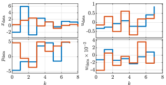
Figure 1: Data-set used for synthesis. The blue lines represent the first elements of $x,u,p$ and $w$, while the red lines represent the second elements.

In order to obtain a representation of the disturbance, we choose $\Pi=\mathrm{blkdiag}(Q,-I_{{N_{\mathrm{d}}}})$ with $Q=10^{-3}\begin{bmatrix}1.78&1.24\\ 1.24&4.68\end{bmatrix}$, which has been obtained by solving $\min_{Q}\mathrm{trace}(Q)$ subject to (10). Let us abbreviate the synthesis problem of Theorem 2 by BLF (indicating a Biquadratic Lyapunov Function), and the synthesis problem in [20, Eq. (32)] by SLF (indicating a Shared Lyapunov Function). Using only the data-set, the vertices of $\mathbb{P}$ and $\Pi$, we solve the BLF and SLF synthesis problems for $\delta=\{1,5\}$ using YALMIP with the MOSEK SDP solver in Matlab. Note that SLF returns a polytopic $K(p)$, which can be easily transformed back to the affine form of (12b) with [20, Eq. (4)]. For $\delta=1$, both problems are successfully solved and indeed yield a stable closed-loop response for both BLF and SLF-based controllers, as shown in the left column of Fig. 2.

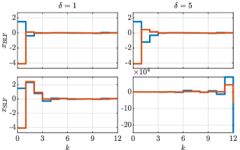
Figure 2: Closed-loop simulation with the synthesized BLF (first row) and SLF (second row) based controllers for $\delta=1$ (left column) and $\delta=5$ (right column). The blue lines represent the first element of $x$, while the red lines represent the second element of $x$. The simulation is under noisy $w_{k}\sim\mathcal{U}(-w_{\max},w_{\max})$.

For $\delta=5$, the BLF synthesis problem is successfully solved. However, the SLF could not find a stabilizing controller for this larger $\mathbb{P}$, and thus results in an unstable closed-loop, as depicted in the plots in the right column of Fig. 2. This shows that the decoupling of the parameter variation from the noise gives more flexibility, at the cost of computational complexity, cf. Remark 4.v.

Moreover, note that our analysis proves that the closed-loop corresponding to any system compatible with the data in Fig. 1 is stable, not just the true system. To illustrate the difficulty, and the different behaviors shown by the systems we stabilize, Fig. 3 shows a number of trajectories,

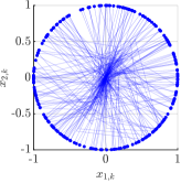
Figure 3: 232 closed-loop responses of an arbitrary system compatible with the data and an initial condition on the unit circle. Here $w_{k}\equiv 0$ for the closed-loop simulations.

each corresponding to a random initial condition on the unit circle and a random system compatible with the data in closed-loop with the controller synthesized for $\delta=5$. This further emphasizes the robustness of the approach.

To show the robustness against $w$ resulting from the aforementioned decoupling is demonstrated by computing the closed-loop $\ell_{2}$-gain for different values of $w_{\max}$, where the controller is synthesized for $\delta=1$. The results are shown in Table I.

Table I: Closed-loop $\ell_{2}$-gain for different values of $w_{\max}$.

$w_{\max}$	0.01	0.21	0.41	0.60	0.80	1.00
$\ell_{2}$-gain $\times 10$ (BLF)	0.11	2.36	4.61	6.86	9.11	11.4
$\ell_{2}$-gain $\times 10$ (SLF)	0.49	10.2	12.0	29.7	39.5	49.2

Although the controllers have not been designed to minimize the closed-loop $\ell_{2}$-gain, the rate at which the closed-loop $\ell_{2}$-gain increases over increasing $w_{\max}$ gives a good indication of the robustness against $w$. The results of Table I show that the rate at which the closed-loop with the SLF-based controller increases much faster than with the BLF-based controller. This indicates that the data-driven controllers synthesized with the methods in this paper achieve much better attenuation of the disturbance.

VII Conclusions

In this paper, we developed LPV controller synthesis methods that guarantee Lyapunov stability of the closed-loop system using biquadratic Lyapunov functions, which are less conservative than common Lyapunov functions. The LPV controllers are synthesized using only a single sequence of noisy data, where we assume that the noise admits a QMI. Formulation of these results is made possible by the adaptation of the LPV framework in the informativity framework, merged with the use of biquadratic Lyapunov functions in LPV controller synthesis. The simulation example demonstrates the increased robustness of the synthesized controllers compared to the controllers synthesized with common Lyapunov functions. As a future work, we aim to extend the data-driven state-feedback methods to include performance objectives, such as $\ell_{2},\mathcal{H}_{2}$, passivity, etc. Furthermore, similar data-driven approaches with output feedback LPV controllers are of interest.

References

- [1] “Data-driven control: Part I & Part II,” IEEE Control Systems Magazine, vol. 43, no. 5,6, 2023.
- [2] F. Dörfler, “Data-driven control: Part two of two: Hot take: Why not go with models?” IEEE Control Systems Magazine, vol. 43, no. 6, pp. 27–31, 2023.
- [3] J. C. Willems, P. Rapisarda, I. Markovsky, and B. L. M. De Moor, “A note on persistency of excitation,” Systems & Control Letters, vol. 54, no. 4, pp. 325–329, 2005.
- [4] H. J. van Waarde, J. Eising, H. L. Trentelman, and M. K. Camlibel, “Data informativity: a new perspective on data-driven analysis and control,” IEEE Trans. on Automatic Control, vol. 65, no. 11, pp. 4753–4768, 2020.
- [5] J. Eising and H. L. Trentelman, “Informativity of noisy data for structural properties of linear systems,” Systems & Control Letters, vol. 158, p. 105058, 2021.
- [6] I. Markovsky and F. Dörfler, “Identifiability in the behavioral setting,” IEEE Trans. on Automatic Control, vol. 68, pp. 1667–1677, 2022.
- [7] C. De Persis, D. Gadginmath, F. Pasqualetti, and P. Tesi, “Data-driven feedback linearization with complete dictionaries,” in Proc. of the 62nd IEEE Conf. on Decision and Control, 2023, pp. 3037–3042.
- [8] M. Alsalti, J. Berberich, V. G. Lopez, F. Allgöwer, and M. A. Müller, “Data-based system analysis and control of flat nonlinear systems,” in Proc. of the 60th IEEE Conf. on Decision and Control, 2021, pp. 1484–1489.
- [9] M. Guo, C. De Persis, and P. Tesi, “Data-driven stabilization of nonlinear polynomial systems with noisy data,” IEEE Trans. on Automatic Control, vol. 67, no. 8, pp. 4210–4217, 2021.
- [10] I. Markovsky, “Data-driven simulation of generalized bilinear systems via linear time-invariant embedding,” IEEE Trans. on Automatic Control, vol. 68, no. 2, pp. 1101–1106, 2022.
- [11] J. Eising and J. Cortes, “Cautious optimization via data informativity,” arXiv preprint arXiv:2307.10232, 2023.
- [12] M. Lazar, “Basis functions nonlinear data-enabled predictive control: Consistent and computationally efficient formulations,” arXiv preprint arXiv:2311.05360, 2023.
- [13] S. Formentin, D. Piga, R. Tóth, and S. M. Savaresi, “Direct data-driven control of linear parameter-varying systems,” in Proc. of the 52nd IEEE Conf. on Decision and Control, 2013, pp. 4110–4115.
- [14] Y. Bao and J. M. Velni, “An overview of data-driven modeling and learning-based control design methods for nonlinear systems in LPV framework,” in Proc. of the 5th IFAC Workshop Linear Parameter Varying Systems, 2022, pp. 1–10.
- [15] C. Hoffmann and H. Werner, “A survey of linear parameter-varying control applications validated by experiments or high-fidelity simulations,” IEEE Trans. on Control Systems Technology, vol. 23, no. 2, pp. 416–433, 2014.
- [16] R. Tóth, Modeling and Identification of Linear Parameter-Varying Systems, ser. Lecture Notes in Control and Information Sciences. Heidelberg: Springer, 2010, vol. 403.
- [17] C. Verhoek, H. S. Abbas, and R. Tóth, “Direct data-driven LPV control of nonlinear systems: An experimental result,” in Proc. of the 22nd IFAC World Congress 2023, 2023, pp. 2263–2268.
- [18] C. Verhoek, P. J. W. Koelewijn, S. Haesaert, and R. Tóth, “Direct data-driven state-feedback control of general nonlinear systems,” in Proc. of the 62nd IEEE Conf. on Decision and Control, 2023, pp. 3688–3693.
- [19] C. Verhoek, R. Tóth, S. Haesaert, and A. Koch, “Fundamental lemma for data-driven analysis of linear parameter-varying systems,” in Proc. of the 60th IEEE Conf. on Decision and Control, 2021, pp. 5040–5046.
- [20] J. Miller and M. Sznaier, “Data-driven gain scheduling control of linear parameter-varying systems using quadratic matrix inequalities,” IEEE Control Systems Letters, vol. 7, pp. 835–840, 2022.
- [21] R. Tóth, H. S. Abbas, and H. Werner, “On the state-space realization of LPV input-output models: Practical approaches,” IEEE Trans. on Control Systems Technology, vol. 20, no. 1, pp. 139–153, 2011.
- [22] C. Verhoek, R. Tóth, and H. S. Abbas, “Direct data-driven state-feedback control of linear parameter-varying systems,” arXiv preprint arXiv:2211.17182, 2022.
- [23] H. J. van Waarde, M. K. Camlibel, J. Eising, and H. L. Trentelman, “Quadratic matrix inequalities with applications to data-based control,” SIAM Journal on Control and Optimization, vol. 61, no. 4, pp. 2251–2281, 2023.
- [24] P. Koelewijn, G. S. Mazzoccante, R. Tóth, and S. Weiland, “Pitfalls of guaranteeing asymptotic stability in LPV control of nonlinear systems,” in Proc. of the 2020 European Control Conf., 2020, pp. 1573–1578.
- [25] M.-D. Choi, “Positive semidefinite biquadratic forms,” Linear Algebra and its Applications, vol. 12, no. 2, pp. 95–100, 1975.
- [26] C. E. de Souza and A. Trofino, “Gain-scheduled controller synthesis for linear parameter varying systems via parameter-dependent Lyapunov functions,” International Journal of Robust and Nonlinear Control, vol. 16, no. 5, pp. 243–257, 2006.
- [27] C. Scherer, “LPV control and full block multipliers,” Automatica, vol. 27, no. 3, pp. 325–485, 2001.
- [28] C. Scherer and S. Weiland, “Linear matrix inequalities in control,” Lecture Notes, Dutch Institute for Systems and Control, Delft, The Netherlands, 2021.
- [29] F. Wu and K. Dong, “Gain-scheduling control of LFT systems using parameter-dependent Lyapunov functions,” Automatica, vol. 42, no. 1, pp. 39–50, 2006.
- [30] P. den Boef, P. B. Cox, and R. Tóth, “LPVcore: Matlab toolbox for LPV modelling, identification and control of non-linear systems,” in Proc. of the 19th Symp. on System Identification, 2021, pp. 385–390.