FedFixer: Mitigating Heterogeneous Label Noise in Federated Learning

Abstract

Federated Learning (FL) heavily depends on label quality for its performance. However, the label distribution among individual clients is always both noisy and heterogeneous. The high loss incurred by client-specific samples in heterogeneous label noise poses challenges for distinguishing between client-specific and noisy label samples, impacting the effectiveness of existing label noise learning approaches. To tackle this issue, we propose FedFixer, where the personalized model is introduced to cooperate with the global model to effectively select clean client-specific samples. In the dual models, updating the personalized model solely at a local level can lead to overfitting on noisy data due to limited samples, consequently affecting both the local and global models’ performance. To mitigate overfitting, we address this concern from two perspectives. Firstly, we employ a confidence regularizer to alleviate the impact of unconfident predictions caused by label noise. Secondly, a distance regularizer is implemented to constrain the disparity between the personalized and global models. We validate the effectiveness of FedFixer through extensive experiments on benchmark datasets. The results demonstrate that FedFixer can perform well in filtering noisy label samples on different clients, especially in highly heterogeneous label noise scenarios.

Introduction

Federated Learning (FL) aims to learn a common model from different clients while maintaining client data privacy, and it has gradually been applied to real-world applications (Li et al. 2020; He et al. 2020, 2019; Pu et al. 2023a). However, the presence of heterogeneous label noise (Li et al. 2019, 2021b; Zhu et al. 2021) in each local client severely degrades the generalization performance of FL models (Wang et al. 2022).

Unlike Centralized Learning (CL) with noisy labels (Zhu et al. 2023; Zhu, Wang, and Liu 2022; Zhu, Dong, and Liu 2022), FL confronts a unique situation where each client’s label noise distributionmay be heterogeneous due to variations in the true class distribution and personalized human labeling errors (Wei et al. 2022; Han et al. 2018; Yi et al. 2022). Fig. 1(a) visually demonstrates significant differences in the label noise distribution between client $p$ and client $q$. Consequently, the existence of heterogeneous label noise severely degrades the generalization performance of FL model (Wang et al. 2022), leading to an even more pronounced impact on FL compared to CL with noisy labels, as shown in Fig. 1(b). Therefore, there is a critical need for a robust label noise learning method tailored to FL to address this challenge effectively.

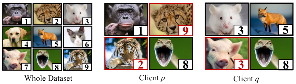
(a) Label noise distribution on client $p$ and $q$. Black are correct labels and Red are noisy labels.

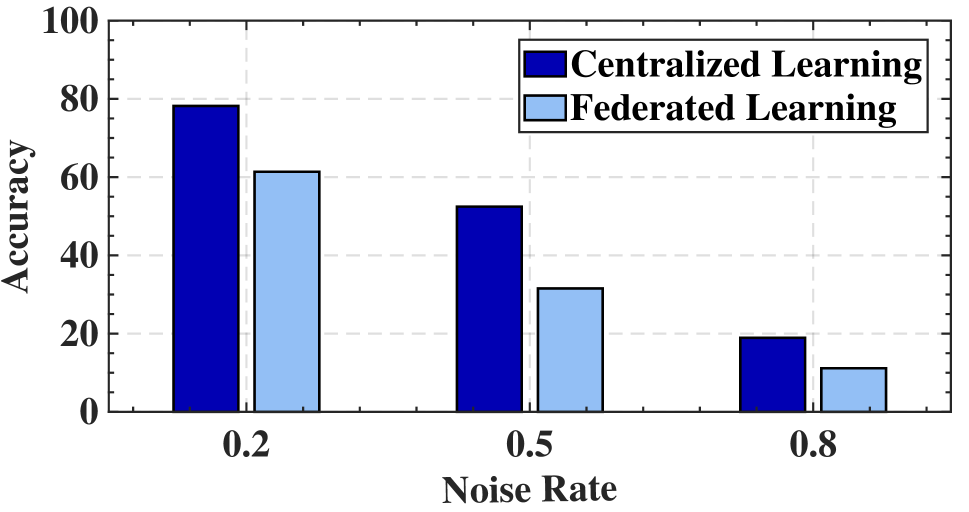
(b) CL with noisy labels & FL with heterogeneous noisy labels.

Figure 1: (a): The heterogeneous label noise distributions encompass diverse true class samples or varying label noise transitions. (b): The performance comparison between CL and FL on CIFAR-10 with the rate of label noise 0.2, 0.5, and 0.8.

Numerous research efforts have been devoted to addressing noisy labels in CL (Cheng et al. 2021; Li, Socher, and Hoi 2019; Liu and Guo 2020; Natarajan et al. 2013; Wei et al. 2020). However, when directly applied to FL, these CL-based methods encounter significant challenges. For instance, learning a model using local noisy label data on the client side is susceptible to overfitting due to the limited sample size. Furthermore, training a global model through FedAvg (McMahan et al. 2017) struggles to effectively learn client-specific samples, potentially leading to difficulties in correctly identifying whether high-loss samples are noisy label samples or client-specific samples. Moreover, existing methods designed for the issue of label noise in FL can be broadly categorized into coarse-grained (Chen et al. 2020; Li et al. 2021a; Yang et al. 2021) and fine-grained (Tuor et al. 2021; Xu et al. 2022) methods. However, these methods usually ignore the heterogeneity of noisy label samples in FL. They encounter difficulty in the personalized identification of noisy label samples across diverse clients. This difficulty impairs their potential to achieve substantial performance improvements. It is challenging to effectively recognize wrongly labeled samples from different clients in FL.

In this paper, we propose FedFixer, an FL algorithm with the dual model structure to mitigate the impact of heterogeneous noisy label samples in FL. FedFixer consists of two models: the global model ($w$) and the auxiliary personalized model ($\theta$). During the local training process at each client, the global model $w$ and personalized model $\theta$ are alternately updated using the samples selected by each other. With alternative updates of dual models, FedFixer can effectively decrease the risk of error accumulation from a single model over time. Unfortunately, unlike the global model which benefits from updates through aggregation, the local updates of the personalized model are prone to overfitting on noisy label data due to being confined to a limited sample size. This susceptibility to overfitting has negative implications on the overall performance of the dual model structure. To alleviate the overfitting in the dual models, it can be addressed from two different perspectives. First, we employ a confidence regularizer to alleviate the unconfident predictions induced by label noise. Second, we implement a distance regularizer between the parameters of the personalized model and the global model to counter the risk of the personalized denoising model overfitting local data.

Our contributions can be summarized as follows:

1. Dual Model Structure: Our tailored dual model structure for FL with heterogeneous label noise effectively adapts to heterogeneous label noise distributions, addressing challenges from varying true class distributions and personalized human labeling errors.

2. Regularization Terms: To combat the overfitting of dual models, we first employ the confidence regularizer to restrict unconfident predictions caused by label noise. Secondly, we implement a distance regularizer into the dual model structure to constrain model distance with the global model.

3. Extensive Experimental Validation: Validated on the benchmark datasets with multiple clients and varying degrees of label noise, FedFixer demonstrates comparable performance to state-of-the-art (SOTA) methods in general scenarios with heterogeneous noisy labels. However, in highly heterogeneous label noise scenarios, our method outperforms existing SOTA methods by up to 10%, showcasing its effectiveness in addressing heterogeneous label noise in FL.

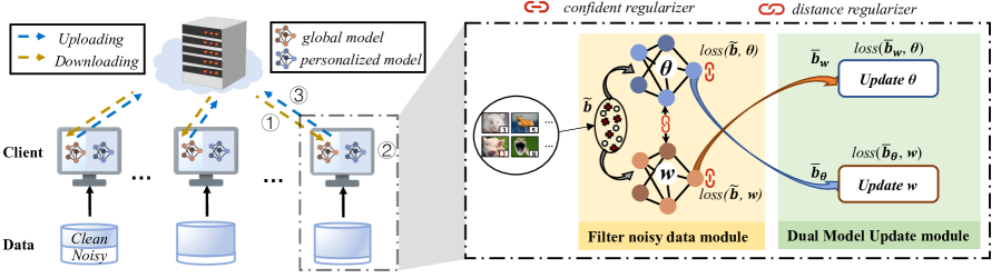
Figure 2: Overall architecture. The training process of the proposed FedFixer has three stages: ① deployment of the global model, ② the local model updates, and ③ the global model aggregation. In the second stage, dual models are alternately updated (in the Dual Model Update module) based on the selected samples (in the Filter Noisy Data module) by each other.

Related Work

In this section, we review the related works. We first discuss existing robust FL methods that address label noise. Additionally, we introduce the related work of learning with noisy labels in a centralized setting.

Robust FL

Robust FL has been extensively studied, and it can be categorized into client-level and sample-level methods. For client-level approaches, Yang et al. (Yang et al. 2021) proposed an online client selection framework that efficiently selects a client set with low noise ratios using Copeland score and multi-arm bandits. Similarly, Fang et al. (Fang and Ye 2022) provided the RHFL to address FL problem with noisy and heterogeneous clients. On the other hand, sample-level methods focus on reducing noisy label samples from local data. Tuor et al. (Tuor et al. 2021) proposed a method for the distributed method to select relevant samples, where the high-relevance data samples at each client are identified using a benchmark model trained on a small benchmark dataset, improving model’s generalization ability (Pu et al. 2021, 2022, 2023b). Xu et al. (Xu et al. 2022) proposed FedCorr, a general multi-stage framework. The initial step involves the detection of clean client sets using GMM(Gaussian Mixture Models) (Pu et al. 2020). Subsequently, model fine-tuning is performed on these clean client sets, and the corrected label samples are relabeled. Finally, the federated model is trained using the conventional FL stage. However, these existing methods can’t effectively address the challenge of heterogeneous label noise in FL. In contrast, our work proposes a dual model structure approach to effectively adapt to heterogeneous label noise distributions to address this challenge.

Learning with Noisy Labels

Learning with noisy labels is a well-studied area, primarily focused on centralized learning (Zhu, Liu, and Liu 2021; Zhu, Song, and Liu 2021; Cheng et al. 2023; Wei et al. 2023). Existing approaches can be categorized into several categories, including Robust Architecture (Goldberger and Ben-Reuven 2017; Lee et al. 2019), Robust Regularization (Xia et al. 2020; Gudovskiy et al. 2021), Robust Loss Design (Ghosh, Kumar, and Sastry 2017; Pu, Zhong, and Sebe 2023; Jiang et al. 2021), and Sample Selection (Jiang et al. 2018; Han et al. 2018; Cheng et al. 2021). In this paper, we specifically review Sample Selection methods, which have gained attention due to the theoretical and empirical exploration of DNNs’ memorization properties to identify clean examples from noisy training data (Xia et al. 2020; Liu et al. 2020). For instance, Han et al. proposed the “Co-teaching” deep learning paradigm to combat noisy labels, while Cheng et al. proposed CORES², which progressively sieves out corrupted examples. Additionally, Xia et al. (Xia et al. 2020) proposed robust early-learning to reduce the side effects of noisy labels before early stopping and enhance the memorization of clean labels. While existing research has achieved promising results in noisy label learning within the centralized learning framework, direct application of these approaches to FL is challenging. This is due to the limited sample size and the heterogeneous label noise distribution, which can result in uncertain performance for each client. Therefore, our proposed method specifically addresses these challenges to effectively handle heterogeneous label noise in FL.

Problem Definition

In this section, we formulate the problem of FL with heterogeneous label noise. Consider a large collection of data $D$ with a sample size of $N$ and $L$ class labels, which is distributed over $K$ clients that $D=\cup_{k=1}^{K}D^{k}:=\cup_{k=1}^{K}\left\{(x^{k}_{n},y^{k}_{n})\right\}_{n\in[n_{k}]}$, where $[n_{k}]=\left\{1,2,...,n_{k}\right\}$ is the set of example indices on client $k$. Each local instance $(x^{k}_{n},y^{k}_{n})\in D^{k}$ follows the data distribution $(X^{k},Y^{k})\sim\mathcal{D}^{k}$. If the distributions $\mathcal{D}^{k}=\mathcal{D},\forall k\in[K]$, we call the samples from all clients are Independent and Identically Distributed (IID); otherwise, they are non-IID. We consider non-IID distribution like (McMahan et al. 2017), where the label space on client $k$ is a subset of the total label space [$L$]. In real-world scenarios, label information from human annotators can be imperfect (Wei et al. 2022), leading to noisy labels $\tilde{y}_{n}$ that may or may not be identical to the true labels $y_{n}$. If $\tilde{y}_{n}\neq{y}_{n}$, we say $\tilde{y}_{n}$ is corrupted, otherwise it is clean. Assume the label noise is class-dependent (Natarajan et al. 2013; Liu and Tao 2015; Liu and Guo 2020). Then for each client $k$, we can use the noise transition matrix $T^{k}$ to capture the transition probability from clean label $Y=y$ to noisy label $\widetilde{Y}=\tilde{y}$. Specifically, we have the following definition:

Definition (Client-Dependent Label Noise).

The label noise on clients $\{1,\cdots,K\}$ is client-dependent if the label noise on each client $k$ can be characterized by noise transition matrix $T^{k}$, where each element satisfies:

$$\forall k\in[K],i,j\in[L],T^{k}_{ij}:=\mathbb{P}_{(X,Y)\sim\mathcal{D}^{k}}(\widetilde{Y}=j|Y=i).$$

When $\mathcal{D}^{k}=\mathcal{D}$ and $T_{k}=T,\forall k\in[K]$, we refer to the label noise distribution among clients as homogeneous, otherwise, they are considered heterogeneous. This means that the heterogeneity of label noise distribution among clients primarily depends on the distribution of true labels and the associated label noise transition based on the true labels. For instance, if the noise transition matrix $T^{k},k=1,..,K$ are heterogeneous, label noise distributions among clients are heterogeneous even if the distributions of true labels among clients are the same (as in the case of IID distribution).

FedFixer: Dual Model Structure Approach

In this section, we introduce FedFixer, the proposed dual structure approach to effectively train the FL model by identifying and filtering noisy label samples on clients.

Dual Model Structure

We present a novel dual model structure, illustrated in Fig. 2, inspired by the well-known noisy label learning method Co-teaching (Han et al. 2018). The objective of FedFixer is:

$$\min_{w}\left\{F(w)\triangleq\sum_{k=1}^{K}\frac{\bar{n}_{k}}{\bar{n}}F_{k}(w)\right\}$$ (1)

where $w$ is the parameters of the global model, $\frac{\bar{n}_{k}}{\bar{n}}$ is the weight of the $k$-th device, $\frac{\bar{n}_{k}}{\bar{n}}\geq 0$, and $\sum_{k}\bar{n}_{k}=\bar{n}$. Here, $\bar{n}_{k}$ is the number of selected samples on $k$-th client and $\bar{n}$ is the sum of selected samples on all clients. For client $k$, $F_{k}(\cdot)$ represents the local optimization objective, which measures the loss of predictions on local data. It is defined as follows:

$$F_{k}(w)=\frac{1}{\bar{n}_{k}}\sum_{n\in[n_{k}]}v_{n}\cdot\ell(x_{n},\tilde{y}_{n};\theta_{k})+\frac{\lambda}{2}\left\|\theta_{k}-w\right\|^{2}$$ (2)

where $v_{n}\in\left\{0,1\right\}$ indicates whether example $n$ is clean ($v_{n}=1$) or not ($v_{n}=0$), and $\ell(\cdot)$ is the loss function. Towards the optimization objective, the training process of FedFixer comprises three stages:

• Step-1: The selected clients download the global model $w$ from the server. The number of selected clients is determined by $C$, which is the fraction of a fixed set of $K$ clients in each round.

• Step-2: At each client, the training process involves updating the dual models locally with the selected clean samples for $E$ epochs.

• Step-3: The locally-computed parameter updates $\nabla w_{t}$ of the global model $w$ will be uploaded to the server for aggregation.

There are dual models on each client for local updates of Step-2. On client $k$, the dual models are denoted the global model $w_{k}$ and personalized model $\theta_{k}$. The loss function on the dual models on the batch data $\tilde{b}$ is denoted as $\ell(\tilde{b})$, where the loss of the global model is $\ell(\tilde{b};w_{k})$, and the loss of personalized model is $\ell(\tilde{b};\theta_{k})$. When a batch $\tilde{b}$ arrives, the personalized model $\theta_{k}$ and global model $w_{k}$ in the ‘Filter Noisy Data’ module respectively select a small proportion of low loss samples out of the mini-batch $\tilde{b}$ by sample selector defined in Eq. (3), denoted as $\bar{b}_{\theta_{k}}$ and $\bar{b}_{w_{k}}$.

$$v_{n}=\mathds{1}\!\left(\!\ell_{CE}\left(f\left(x_{n}\right),\tilde{y}_{n}\right)-\frac{1}{L}\sum_{\tilde{y}\in[L]}\!\ell_{CE}\left(f\left(x_{n}\right),\tilde{y}\right)\!<\!0\!\right)$$ (3)

where $f(\cdot)$ denotes the logistical output of a classifier, and $\ell_{CE}(\cdot)$ is the Cross Entropy (CE) loss. By employing the indicator function $\mathds{1}(\cdot)$, the sample selector determine $v_{n}=1$ when $\ell_{CE}\left(f\left(x_{n}\right),\tilde{y}_{n}\right)-\frac{1}{L}\sum_{\tilde{y}\in[L]}\!\ell_{CE}\left(f\left(x_{n}\right),\tilde{y}\right)<0$, otherwise $v_{n}=0$. The sample selector is used to judge whether the CE loss of the sample deviates from the mean of the sample’s prediction distribution. The quality of selecting clean examples is guaranteed in Theorem 1.

Theorem 1.

The sample selector defined in (3) ensures that clean examples ($x_{n}$, $\tilde{y}_{n}=y_{n}$) will not be identified as noisy label samples if the model $f(\cdot)$’s prediction on $x_{n}$ is better than a random guess.

Finally, the selected instances are fed into its peer model to generate the loss in the ‘Dual Model Update’ module, denoted as $\ell(\bar{b}_{\theta_{k}};w_{k})$ and $\ell(\bar{b}_{w_{k}};\theta_{k})$ for alternate parameter updates.

In the dual model structure, the global model $w$ and the personalized model $\theta$ inherently incorporate distinct different prior knowledge. Through updates based on mutual insights, both models can identify and filter out mislabeled instances. The global model $w$ can be updated through local updates and global aggregation. On the contrary, if the personalized model $\theta$ is only updated solely based on the local client’s data, it is prone to overfitting due to the limited amount of data available. This overfitting can hurt the overall performance of the dual models. Therefore, we introduce the regularizers to prevent the overfitting of dual models, as discussed in the following subsections.

Regularizers

Confidence Regularizer

Effectively selecting clean label samples is crucial. The commonly used Cross Entropy (CE) loss is inadequate for learning models with noisy label samples (Ghosh, Kumar, and Sastry 2017). This could magnify the overfitting inclination of inherently susceptible personalized model in the dual models. To address this, we introduce the Confidence Regularizer (CR) (Cheng et al. 2021), defined in Eq. (4), as a modification to the vanilla CE loss. This incorporation aims to guide the model towards better fitting clean datasets.

$$\ell_{\mathrm{CR}}\left(f\left(x_{n}\right)\right):=-\beta\cdot\mathbb{E}_{\mathcal{D}_{\widetilde{Y}\mid\text{$\widetilde{D}$}}}\left[\ell_{CE}\left(f\left(x_{n}\right),\widetilde{Y}\right)\right]$$ (4)

Here, $\beta\geq 0$ represents a hyperparameter, and the prior probability $\mathbb{P}(\widetilde{Y}\!\!\mid\!\!\widetilde{D})$ is determined based on the noisy dataset, i.e., $\mathbb{P}(\tilde{Y}=i)=\#\text{Label}\_i/N$ ($\#\text{Label}\_i$ is the number of samples for $i$-th class label, and N is the total number of samples). The incorporation of the CR leads to the following objective:

$$\min\limits_{\begin{subarray}{c}f\in\mathcal{F},\\ v\in\{0,1\}^{n_{k}}\end{subarray}} \,\frac{1}{\bar{n}_{k}}\sum\limits_{n\in[n_{k}]}v_{n}\left[\ell_{CE}\left(f\left(x_{n}\!\right),\tilde{y}_{n}\right)+\ell_{CR}\left(f\left(x_{n}\right)\right)\right]$$ (5)

$$s.t. \ell_{CR}\left(f\left(x_{n}\right)\right):=-\beta\cdot\mathbb{E}_{\mathcal{D}_{\tilde{Y}\mid\widetilde{D}}}\ell\left(f\left(x_{n}\right),\widetilde{Y}\right)$$

The training of dual models is performed using the function $\ell(\cdot)=\ell_{CE}(\cdot)+\ell_{CR}(\cdot)$, and the sample selector defined in Eq. (3) is used to differentiate between noisy and clean samples. Throughout the paper, we use $\ell(\cdot)$ to refer to $\ell_{CE}(\cdot)+\ell_{CR}(\cdot)$ by default. Consequently, the model can be updated on $(x_{n},\bar{y}_{n})$ according to Eq. (6), where $(x_{n},\bar{y}_{n})$ is the sample selected by sample selector.

$$f=\underset{f\in\mathcal{F}}{\arg\min}\frac{1}{\bar{n}_{k}}\underset{n\in[\bar{n}_{k}]}{\sum}\ell_{CE}\left(f\left(x_{n}\right),\bar{y}_{n}\right)+\ell_{\mathrm{CR}}\left(f\left(x_{n}\right)\right)$$ (6)

With the CR, the dual models’ personalized model $\theta$ and global model $w$ can effectively, to a certain extent, avoid overfitting to noisy label samples. Subsequently, they update their parameters according to Eq. (6) using the selected samples, as determined by the sample selector constructed by their peer model. However, it doesn’t fundamentally address the issue of overfitting to local noisy data within the personalized model of the dual models. Consequently, the personalized model’s updates drift farther away from the global model, causing the dual model structure to deteriorate. Therefore, we introduce a distance regularizer to effectively control this deviation.

Distance Regularizer

Instead of directly optimizing the objective (5), we can optimize the objective (2) by incorporating a Distance Regularizer (DR) into the loss function for each client. The DR can be defined as follows:

$$\frac{\lambda}{2}\left\|\theta_{k}-w\right\|^{2}$$ (7)

where $\theta_{k}$ denotes the personalized model of client $k$, and $\lambda\in(0,+\infty)$ is a regularization parameter that governs the influence of the global model $w$ on the personalized model. A larger value of $\lambda$ enhances the benefits of the personalized model from the global model, while a smaller value encourages the personalized model to pay more attention to local information. For solving objective (2), each client $k$ obtains its personalized model $\theta_{k}(w_{k})$ through the update equation:

$$\theta_{k}(w_{k})\leftarrow\theta_{k}-\zeta(\bigtriangledown\ell_{k}\left(\theta_{k}\right)+\lambda(\theta_{k}-w_{k}))$$ (8)

where $w_{k}$ is constant and refers to the local model of the client $k$, and $\zeta$, represents the personalized learning rate. Additionally, the global model of client $k$ is updated using:

$$w_{k}\leftarrow w_{k}-\eta\lambda(w_{k}-\theta(w_{k}))$$ (9)

where $\eta$ denotes the global learning rate.

Please note that the previous updates of the global model in Eq. (9) on clients are solely for solving the problem (7). However, it is crucial to emphasize that the global model should also be carried out for alternate updates, as illustrated in Algorithm 1 (line 25).

Input: $T$, $T_{s}$, $E$, $\lambda$, $\eta$, $\zeta$, $\gamma$, $B$, $K$, $w$.

Output: $w$, $\theta_{i},i=1,...,K$.

1

2Server executes:

3 initialize $w_{0}$

4 for each round $t$ from 0 to $T-1$ do

5       $m\leftarrow\max(C\cdot K,1)$

6       $\mathcal{S}_{t}$ $\leftarrow$ (random set of $m$ clients)

7       for each client $k\in\mathcal{S}_{t}$ in parallel do

8             $\bar{n}_{k}$, $w_{t+1}^{k}\leftarrow$ ClientUpdate$(t,k,w_{t})$

9       end for

10      $w_{t+1}\leftarrow(1-\gamma)w_{t}+\gamma\sum_{k\in|\mathcal{S}_{t}|}\frac{\bar{n}_{k}}{\bar{n}}w_{t+1}^{k}$

11 end for

12

13Client executes: /* Run on client $k$ */

14 ClientUpdate($t$, $k$, $w$):

15 $\mathcal{\tilde{B}}\leftarrow$ (split $\tilde{D}_{k}$ into batches of size $B$)

16 $\theta\leftarrow\textit{deepcopy}(w)$

17 for each local epoch $i$ from 1 to $E$ do

18       for batch $\tilde{b}^{j}\in\mathcal{\tilde{B}}$ do

19             if $t\leq T_{s}$ then

20                   $\bar{b}_{w}^{j}=\bar{b}_{\theta}^{j}=\tilde{b}^{j}$

21                  

22            else

23                   $\bar{b}_{w}^{j}=Selector\,\ell_{CE}(\tilde{b};w)$

24                  

25                  $\bar{b}_{\theta}^{j}=Selector\,\ell_{CE}(\tilde{b};\theta)$

26                  

27             end if

28            

29            $\theta(w)\leftarrow\theta-\zeta(\bigtriangledown\ell(\bar{b}_{w}^{j};\theta)+\lambda(\theta-w))$

30             $w\leftarrow w-\eta\lambda(w-\theta(w))$

31            

32            $w\leftarrow w-\eta\bigtriangledown\ell(\bar{b}_{\theta}^{j};w)$

33       end for

34      

35      $\bar{n}_{k}^{i}=\sum_{j=1}^{B}|\bar{b}_{\theta}^{j}|$

36 end for

37

38$\bar{n}_{k}=\frac{1}{E}\sum_{i=1}^{E}\bar{n}_{k}^{i}$

return $\bar{n}_{k}$, $w$

Algorithm 1 FedFixer.

Dataset	Clothing1M	CIFAR-10	MNIST
Training instances	1,000,000	50,000	60,000
Number of classes	14	10	10
Total clients	300	100	100
Fraction $C$	0.03	0.1	0.1
Learning rate $\eta$	0.001	0.01	0.1
Rounds	50	450	300
Model Architecture	ResNet-50	ResNet-18	LetNet-5

Table 1: Summary of the datasets.

Datasets	Methods	IID			non-IID
		$\rho$ = 0.0	$\rho$ = 0.5	$\rho$ = 1	$\rho$ = 0.0	$\rho$ = 0.5	$\rho$ = 1
		$\tau$ = 0.0	$\tau$ = 0.3	$\tau$ = 0.5	$\tau$ = 0.0	$\tau$ = 0.3	$\tau$ = 0.5
MNIST	Local + CORES2	96.79 $\pm$ 0.05	62.38 $\pm$ 3.88	37.30 $\pm$ 1.62	97.52 $\pm$ 0.17	90.31 $\pm$ 3.29	55.80 $\pm$ 6.45
	Global + CORES2	98.05 $\pm$ 0.05	97.39 $\pm$ 0.13	80.98 $\pm$ 4.78	97.46 $\pm$ 0.53	97.38 $\pm$ 0.12	87.45 $\pm$ 0.48
	FedAvg	98.39 $\pm$ 0.04	97.66 $\pm$ 0.09	93.90 $\pm$ 0.31	97.46 $\pm$ 0.57	97.73 $\pm$ 0.05	95.57 $\pm$ 0.28
	FedProx	98.22 $\pm$ 0.08	96.49 $\pm$ 0.08	93.90 $\pm$ 0.64	93.69 $\pm$ 4.98	97.25 $\pm$ 0.16	95.22 $\pm$ 0.37
	RFL⋆	90.70 $\pm$ 0.54	96.54 $\pm$ 0.12	96.64 $\pm$ 0.08	90.51 $\pm$ 0.36	95.61 $\pm$ 0.34	91.56 $\pm$ 8.37
	MR	97.41 $\pm$ 0.21	95.98 $\pm$ 0.36	88.47 $\pm$ 1.48	97.09 $\pm$ 0.54	95.35 $\pm$ 0.54	90.53 $\pm$ 2.26
	FedCorr⋆	98.68 $\pm$ 0.16	98.09 $\pm$ 0.22	95.67 $\pm$ 0.22	97.49 $\pm$ 0.82	97.75 $\pm$ 0.17	95.75 $\pm$ 0.46
	FedFixer	98.07 $\pm$ 0.02	97.80 $\pm$ 0.18	96.79 $\pm$ 0.92	98.05 $\pm$ 0.06	98.01 $\pm$ 0.18	96.00 $\pm$ 0.24
CIFAR-10	Local + CORES2	84.23 $\pm$ 0.26	67.96 $\pm$ 0.60	22.51 $\pm$ 1.79	86.16 $\pm$ 0.71	68.46 $\pm$ 2.38	26.96 $\pm$ 1.21
	Global + CORES2	91.31 $\pm$ 0.09	85.81 $\pm$ 0.26	54.22 $\pm$ 3.18	90.27 $\pm$ 0.17	86.23 $\pm$ 0.20	35.31 $\pm$ 3.51
	FedAvg	90.33 $\pm$ 0.11	77.93 $\pm$ 0.29	33.87 $\pm$ 0.19	89.82 $\pm$ 0.34	78.30 $\pm$ 0.24	28.77 $\pm$ 0.59
	FedProx	91.12 $\pm$ 0.20	79.33 $\pm$ 0.21	35.38 $\pm$ 0.31	90.50 $\pm$ 0.27	80.13 $\pm$ 0.40	29.63 $\pm$ 1.17
	RFL⋆	85.54 $\pm$ 0.26	84.06 $\pm$ 0.24	54.83 $\pm$ 1.06	83.83 $\pm$ 0.41	83.68 $\pm$ 0.32	49.49 $\pm$ 1.77
	MR	70.65 $\pm$ 1.61	50.02 $\pm$ 2.13	23.67 $\pm$ 1.37	68.80 $\pm$ 0.52	51.46 $\pm$ 1.29	22.23 $\pm$ 1.72
	FedCorr⋆	91.82 $\pm$ 0.22	88.05 $\pm$ 0.69	52.30 $\pm$ 0.91	81.07 $\pm$ 1.06	87.63 $\pm$ 0.64	45.43 $\pm$ 3.36
	FedFixer	90.72 $\pm$ 0.47	87.06 $\pm$ 0.30	62.87 $\pm$ 0.17	89.76 $\pm$ 0.32	87.82 $\pm$ 0.22	59.01 $\pm$ 0.55

Table 2: Average (5 trials) accuracies (%) of various methods on MNIST and CIFAR-10 datasets with IID and non-IID settings at different noise levels ($\rho$: ratio of noisy clients, $\tau$: lower bound of client noise level). The best results are highlighted in bold. Methods trained with label correction are marked by $\star$.

Algorithm	Local + CORES2	Global + CORES2	FedAvg	FedProx	FedCorr⋆	RFL⋆	MR	FedFixer
Acc	53.32	65.18	66.75	66.76	67.50	65.41	50.01	70.52

Table 3: Accuracies (%) of various methods on Clothing1M with non-IID setting.

Dataset	Method	Sampling probability for each class.
		$p$ = 0.3	$p$ = 0.5	$p$ = 0.7	$p$ = 0.9
MNIST	FedAvg	92.20	95.45	95.53	95.14
	FedProx	91.91	93.51	94.89	90.39
	RFL⋆	33.80	94.12	95.57	95.26
	MR	80.72	87.21	92.75	90.60
	FedCorr⋆	93.84	95.15	95.77	95.73
	FedFixer	95.21	95.76	96.32	95.78
CIFAR-10	FedAvg	32.48	35.89	43.88	39.27
	FedProx	34.50	37.00	45.28	40.39
	RFL⋆	45.04	58.03	66.93	66.91
	MR	26.00	29.00	30.74	29.98
	FedCorr⋆	48.69	54.53	61.13	64.60
	FedFixer	51.19	62.86	71.54	72.46

Table 4: Average (5 trials) accuracies (%) of various methods on MNIST and CIFAR-10 datasets with different non-IID settings. The noise level is set to $\rho\!=\!1,\tau\!=\!0.5$ on the MNIST dataset and $\rho\!=\!1,\tau\!=\!0.3$ for the CIFAR-10 dataset.

Experiments

In this section, we begin by conducting experiments on benchmark datasets with different settings of heterogeneous label noise to comprehensively compare the performance of various methods. Next, we design experiments to evaluate the performance of different methods under increasing levels of label noise heterogeneity. Furthermore, we observe and compare the denoising performance of different methods across all clients to assess their denoising stability on each client. Lastly, we conduct an ablation study to evaluate the effectiveness of the individual components within the FedFixer.

Experimental Setup

Baselines

To compare FedFixer with centralized noisy label learning methods applied to local clients (only trained on local data to filter noisy samples) and the server (trained by FedAvg to filter noisy samples), we consider a SOTA method: CORES² (Cheng et al. 2021). We refer to the centralized noisy label learning method applied to local clients as “Local + CORES²”. Similarly, we refer to the centralized method applied to the server as “Global + CORES²”. For reference, we also compare FedFixer with two vanilla methods of FL: FedAvg (McMahan et al. 2017) and FedProx (Li et al. 2020). Furthermore, we also comprehensively compare SOTA federated noisy label learning methods, such as FedCorr (Xu et al. 2022), RFL (Yang et al. 2022), and MR (Tuor et al. 2021).

Implementation Details

We evaluate different methods on MNIST (LeCun et al. 1998), CIFAR-10 (Krizhevsky, Hinton et al. 2009), and Clothing1M (Xiao et al. 2015) datasets with specific rounds, model architectures, total clients, and the fraction of selected clients for each dataset, as summarized in Tab. 1. The performance of various methods is tested based on the data division and noise model used in FedCorr (Xu et al. 2022), where $p\in(0,L]$ denotes the class sampling probability of clients, $\rho\in[0,1]$ denotes the ratio of noisy clients, and $\tau\in[0,1]$ denotes the lower bound for the noise level of a noisy client, which means that the noise level can be determined by sampling from the uniform distribution $U(\tau,1)$. To ensure fairness in the comparison, we set common parameters for all the methods: local epoch $E$ = 5, batch size $B$ = 32, and the local solver SGD. For our FedFixer method, we set $\beta=2$ for CIFAR-10/MNIST, $\beta=1$ for Clothing1M. The learning rate $\zeta$ is set to $\frac{1}{2}\eta$ for MNIST dataset and $\zeta$ = $\eta$ for remaining datasets. Additionally, we set the beginning round of noisy sample filtering $T_{s}=10$, hyperparameters $\gamma=1$, and $\lambda=15$ for all datasets. For other methods, we use the default parameters.

We use test accuracy to evaluate the performance of the FL task and $F$-score to evaluate the performance of label error detection. $F$-score is calculated by $F=\frac{2\times\texttt{Precision}\times\texttt{Recall}}{\texttt{Precision}+\texttt{Recall}}$. The precision and recall can be calculated as $\texttt{Precision}=\frac{\sum_{n\in[N]}\mathds{1}\left(v_{n}=0,\tilde{y}_{n}=y_{n}\right)}{\sum_{n\in[N]}\mathds{1}\left(v_{n}=0\right)}$, $\texttt{Recall}=\frac{\sum_{n\in[N]}\mathds{1}\left(v_{n}=0,\tilde{y}_{n}=y_{n}\right)}{\sum_{n\in[N]}\mathds{1}\left(\tilde{y}_{n}=y_{n}\right)}$, where $v_{n}=1$ indicates that $\tilde{y}_{n}$ is detected as a corrupted label, and $v_{n}=0$ if $\tilde{y}_{n}$ is detected to be clean (Cheng et al. 2021).

(a) IID $\rho$ = 0.5, $\tau$ = 0.3

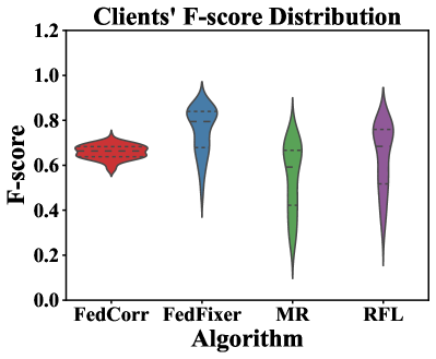
(b) IID $\rho$ = 1, $\tau$ = 0.5

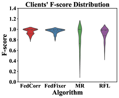
(c) non-IID $\rho$ = 0.5, $\tau$ = 0.3

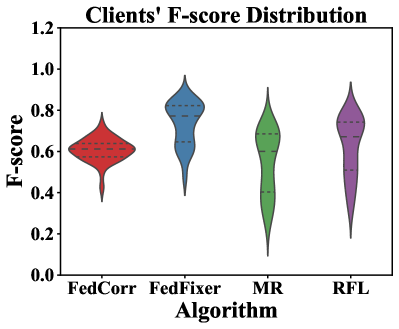
(d) non-IID $\rho$ = 1, $\tau$ = 0.5

Figure 3: Clients’ F-score distribution of different methods on CIFAR-10 with different noise levels on IID and non-IID distribution.

Comparison with State-of-the-Art Methods

Comprehensive Comparison

We compare the prediction performance of FedFixer with all the baseline methods as mentioned above in heterogeneous label noise settings with both IID and non-IID distributions. The results are presented in Tab. 2 for the MNIST, and CIFAR10 datasets. Firstly, we observe that FedFixer consistently achieves excellent accuracy for heterogeneous label noise with IID or non-IID distribution at different noise levels. Secondly, in highly noisy settings, such as IID and non-IID with $\rho$ = 1 and $\tau$ = 0.5, FedFixer significantly outperforms all other methods (especially on CIFAR-10). Furthermore, we notice that the method “Local + CORES²” is almost ineffective and even collapses when directly applied to local clients to filter noisy label samples. Additionally, to assess compatibility, we also test the performance of FedFixer on datasets without noisy label samples. The experimental results show that FedFixer achieves a prediction accuracy similar to FedAvg and FedProx when the noisy label rate is 0.0. Tab. 3 shows the results on Clothing1M, a real dataset with noisy labels. For Clothing1M, FedFixer achieves the highest accuracy.

Robustness with Heterogeneous Label Noise

Tab. 4 presents the performances of various methods as the heterogeneity of label noise increases. The degree of heterogeneity is determined by the sampling probability of each class, denoted as $p$, where $0<p<1$. This probability represents the likelihood of each class being present on each client. As the value of $p$ decreases, the level of label noise heterogeneity increases, creating a more challenging experimental scenario. In Tab. 4, the performances of all methods experience a decline with the increasing heterogeneity of label noise. Our method consistently achieves the highest prediction accuracies across all settings and notably outperforms others on the CIFAR-10 dataset. Different from the observations in Tab. 2, our experiments are always conducted under a high noise setting with $\rho=1$, where the assumption is that all clients possess noisy labels. Under this scenario, the previously effective FedCorr method proves to be ineffective since it relies on the assumption of having a ratio of clean sample clients.

Denoising Stability

Fig. 3 presents the F-score distribution of clients across different algorithms, evaluating the denoising stability on each client. In the violin plots, the distribution of FedFixer and the FedCorr method appears to be highly concentrated, exhibiting consistently high mean values across all the other methods. When compared with FedCorr, our approach exhibits even denser distributions or higher mean values. Although in the IID scenario with $\rho$ = 1 and $\tau$ = 0.5, our approach exhibits a relatively scattered distribution, it still showcases a mean value nearly 0.2 higher than that of FedCorr. Consequently, it demonstrates approximately 10% better predictive performance than FedCorr, as evident from the average test accuracy values in Tab. 2 (IID, $\rho$ = 1, $\tau$ = 0.5). Similarly, in the IID scenario with $\rho$ = 0.5 and $\rho$ = 0.3, our method also exhibits a denser distribution of higher mean values. However, due to our initial approach not incorporating label correction, it shows a predictive accuracy lower by 1% compared to FedCorr. This information can be further referenced in Tab. 2 under the IID scenario with $\rho$ = 0.5 and $\tau$ = 0.3.

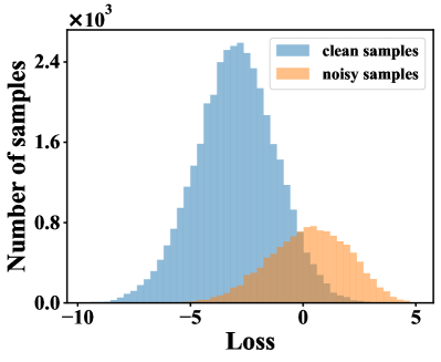
(a) Training without CR.

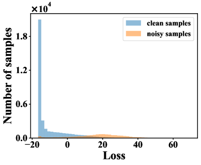
(b) Training with CR.

Figure 4: Loss distribution of clean and noisy samples training without CR and with CR on CIFAR-10 with noise model $\rho=0.5,\tau=0.3$ and IID data partition (Round = 20).

Method	IID		non-IID
	$\rho$ = 0.5	$\rho$ = 1.0	$\rho$ = 0.5	$\rho$ = 1.0
	$\tau$ = 0.3	$\tau$ = 0.5	$\tau$ = 0.3	$\tau$ = 0.5
Ours	87.06	62.87	87.82	59.01
Ours w/o DR	84.45	39.62	83.94	35.74
Ours w/o CR	75.73	35.50	76.29	30.56
Ours w/o AU	86.10	62.62	87.30	54.84
Ours w/o PM	85.47	50.10	85.92	34.44

Table 5: Ablation study results on CIFAR-10.

Ablation Study

Tab. 5 presents an analysis of the effects of different components within FedFixer. This analysis involves evaluating the performance under various scenarios, including ours w/o CR (Confidence Regularizer), ours w/o DR (Distance Regularizer), ours w/o AU (Alternate Updates), and ours w/o PM (Personalized Model). As shown in Tab 5, all these components contribute to performance improvement. The personalized model, in particular, plays a crucial role in scenarios with high levels of heterogeneous label noise. Moreover, Alternate Updates exhibit advantages in high levels of heterogeneous label noise characterized by non-IID distribution. In our dual models, CR has the largest effect. It improves the confidence predictions to effectively distinguish between clean and noisy samples, as depicted in Fig. 4. The DR is also a critical component, preventing the dual models from confusing noisy label samples with client-specific samples.

Conclusions

We introduce FedFixer, a novel and effective dual model structure approach designed to address the issue of heterogeneous label noise in FL. In FedFixer, a personalized model is introduced to learn client-specific samples to decrease the risk of misidentifying client-specific samples as noisy label samples. Moreover, the design of alternative updates of the global model and personalized model can effectively prevent error accumulation from a single model over time. The extensive experiments showcase the superior performance of FedFixer across both IID and non-IID data distribution with label noise, particularly excelling in scenarios with high levels of heterogeneous label noise.

References

- Chen et al. (2020) Chen, Y.; Yang, X.; Qin, X.; Yu, H.; Chan, P.; and Shen, Z. 2020. Dealing with Label Quality Disparity in Federated Learning. In Federated Learning: Privacy and Incentive.
- Cheng et al. (2021) Cheng, H.; Zhu, Z.; Li, X.; Gong, Y.; Sun, X.; and Liu, Y. 2021. Learning with Instance-Dependent Label Noise: A Sample Sieve Approach. In International Conference on Learning Representations.
- Cheng et al. (2023) Cheng, H.; Zhu, Z.; Sun, X.; and Liu, Y. 2023. Mitigating Memorization of Noisy Labels via Regularization between Representations. In International Conference on Learning Representations (ICLR).
- Fang and Ye (2022) Fang, X.; and Ye, M. 2022. Robust Federated Learning With Noisy and Heterogeneous Clients. In Proceedings of the IEEE/CVF Conference on Computer Vision and Pattern Recognition.
- Ghosh, Kumar, and Sastry (2017) Ghosh, A.; Kumar, H.; and Sastry, P. S. 2017. Robust loss functions under label noise for deep neural networks. In Proceedings of the AAAI Conference on Artificial Intelligence.
- Goldberger and Ben-Reuven (2017) Goldberger, J.; and Ben-Reuven, E. 2017. Training deep neural-networks using a noise adaptation layer. In International Conference on Learning Representations.
- Gudovskiy et al. (2021) Gudovskiy, D.; Rigazio, L.; Ishizaka, S.; Kozuka, K.; and Tsukizawa, S. 2021. Autodo: Robust autoaugment for biased data with label noise via scalable probabilistic implicit differentiation. In Proceedings of the IEEE/CVF Conference on Computer Vision and Pattern Recognition.
- Han et al. (2018) Han, B.; Yao, Q.; Yu, X.; Niu, G.; Xu, M.; Hu, W.; Tsang, I.; and Sugiyama, M. 2018. Co-teaching: Robust training of deep neural networks with extremely noisy labels. In International Conference on Neural Information Processing.
- He et al. (2020) He, C.; Li, S.; So, J.; Zeng, X.; Zhang, M.; Wang, H.; Wang, X.; Vepakomma, P.; Singh, A.; Qiu, H.; et al. 2020. Fedml: A research library and benchmark for federated machine learning. preprint arXiv:2007.13518.
- He et al. (2019) He, C.; Tan, C.; Tang, H.; Qiu, S.; and Liu, J. 2019. Central server free federated learning over single-sided trust social networks. preprint arXiv:1910.04956.
- Jiang et al. (2018) Jiang, L.; Zhou, Z.; Leung, T.; Li, L.-J.; and Fei-Fei, L. 2018. Mentornet: Learning data-driven curriculum for very deep neural networks on corrupted labels. In International conference on machine learning.
- Jiang et al. (2021) Jiang, Z.; Zhou, K.; Liu, Z.; Li, L.; Chen, R.; Choi, S.-H.; and Hu, X. 2021. An Information Fusion Approach to Learning with Instance-Dependent Label Noise. In International Conference on Learning Representations.
- Krizhevsky, Hinton et al. (2009) Krizhevsky, A.; Hinton, G.; et al. 2009. Learning multiple layers of features from tiny images. Technical report, Citeseer.
- LeCun et al. (1998) LeCun, Y.; Bottou, L.; Bengio, Y.; and Haffner, P. 1998. Gradient-based learning applied to document recognition. Proceedings of the IEEE, 86(11): 2278–2324.
- Lee et al. (2019) Lee, K.; Yun, S.; Lee, K.; Lee, H.; Li, B.; and Shin, J. 2019. Robust inference via generative classifiers for handling noisy labels. In International conference on machine learning.
- Li, Socher, and Hoi (2019) Li, J.; Socher, R.; and Hoi, S. C. 2019. DivideMix: Learning with Noisy Labels as Semi-supervised Learning. In International Conference on Learning Representations.
- Li et al. (2021a) Li, L.; Fu, H.; Han, B.; Xu, C.-Z.; and Shao, L. 2021a. Federated noisy client learning. preprint arXiv:2106.13239.
- Li et al. (2020) Li, T.; Sahu, A. K.; Zaheer, M.; Sanjabi, M.; Talwalkar, A.; and Smith, V. 2020. Federated optimization in heterogeneous networks. In Proceedings of Machine learning and systems.
- Li et al. (2019) Li, X.; Huang, K.; Yang, W.; Wang, S.; and Zhang, Z. 2019. On the Convergence of FedAvg on Non-IID Data. In International Conference on Learning Representations.
- Li et al. (2021b) Li, X.; Jiang, M.; Zhang, X.; Kamp, M.; and Dou, Q. 2021b. FedBN: Federated Learning on Non-IID Features via Local Batch Normalization. In International Conference on Learning Representations.
- Liu et al. (2020) Liu, S.; Niles-Weed, J.; Razavian, N.; and Fernandez-Granda, C. 2020. Early-learning regularization prevents memorization of noisy labels. In International Conference on Neural Information Processing.
- Liu and Tao (2015) Liu, T.; and Tao, D. 2015. Classification with noisy labels by importance reweighting. IEEE Transactions on pattern analysis and machine intelligence, 38(3): 447–461.
- Liu and Guo (2020) Liu, Y.; and Guo, H. 2020. Peer loss functions: Learning from noisy labels without knowing noise rates. In International conference on machine learning.
- McMahan et al. (2017) McMahan, B.; Moore, E.; Ramage, D.; Hampson, S.; and y Arcas, B. A. 2017. Communication-efficient learning of deep networks from decentralized data. In Artificial intelligence and statistics.
- Natarajan et al. (2013) Natarajan, N.; Dhillon, I. S.; Ravikumar, P. K.; and Tewari, A. 2013. Learning with noisy labels. In International Conference on Neural Information Processing.
- Pu et al. (2020) Pu, N.; Chen, W.; Liu, Y.; Bakker, E. M.; and Lew, M. S. 2020. Dual gaussian-based variational subspace disentanglement for visible-infrared person re-identification. In Proceedings of the 28th ACM International Conference on Multimedia, 2149–2158.
- Pu et al. (2021) Pu, N.; Chen, W.; Liu, Y.; Bakker, E. M.; and Lew, M. S. 2021. Lifelong person re-identification via adaptive knowledge accumulation. In Proceedings of the IEEE/CVF conference on computer vision and pattern recognition, 7901–7910.
- Pu et al. (2022) Pu, N.; Liu, Y.; Chen, W.; Bakker, E. M.; and Lew, M. S. 2022. Meta reconciliation normalization for lifelong person re-identification. In Proceedings of the 30th ACM International Conference on Multimedia, 541–549.
- Pu et al. (2023a) Pu, N.; Zhong, Z.; Ji, X.; and Sebe, N. 2023a. Federated Generalized Category Discovery. arXiv preprint arXiv:2305.14107.
- Pu, Zhong, and Sebe (2023) Pu, N.; Zhong, Z.; and Sebe, N. 2023. Dynamic Conceptional Contrastive Learning for Generalized Category Discovery. In Proceedings of the IEEE/CVF Conference on Computer Vision and Pattern Recognition, 7579–7588.
- Pu et al. (2023b) Pu, N.; Zhong, Z.; Sebe, N.; and Lew, M. S. 2023b. A memorizing and generalizing framework for lifelong person re-identification. IEEE Transactions on Pattern Analysis and Machine Intelligence.
- Tuor et al. (2021) Tuor, T.; Wang, S.; Ko, B. J.; Liu, C.; and Leung, K. K. 2021. Overcoming noisy and irrelevant data in federated learning. In International Conference on Pattern Recognition.
- Wang et al. (2022) Wang, Z.; Zhou, T.; Long, G.; Han, B.; and Jiang, J. 2022. FedNoiL: A Simple Two-Level Sampling Method for Federated Learning with Noisy Labels. preprint arXiv:2205.10110.
- Wei et al. (2020) Wei, H.; Feng, L.; Chen, X.; and An, B. 2020. Combating noisy labels by agreement: A joint training method with co-regularization. In Proceedings of the IEEE/CVF Conference on Computer Vision and Pattern Recognition.
- Wei et al. (2022) Wei, J.; Zhu, Z.; Cheng, H.; Liu, T.; Niu, G.; and Liu, Y. 2022. Learning with Noisy Labels Revisited: A Study Using Real-World Human Annotations. In International Conference on Learning Representations.
- Wei et al. (2023) Wei, J.; Zhu, Z.; Luo, T.; Amid, E.; Kumar, A.; and Liu, Y. 2023. To aggregate or not? learning with separate noisy labels. In ACM SIGKDD Conference on Knowledge Discovery and Data Mining.
- Xia et al. (2020) Xia, X.; Liu, T.; Han, B.; Gong, C.; Wang, N.; Ge, Z.; and Chang, Y. 2020. Robust early-learning: Hindering the memorization of noisy labels. In International Conference on Learning Representations.
- Xiao et al. (2015) Xiao, T.; Xia, T.; Yang, Y.; Huang, C.; and Wang, X. 2015. Learning from massive noisy labeled data for image classification. In Proceedings of the IEEE/CVF Conference on Computer Vision and Pattern Recognition.
- Xu et al. (2022) Xu, J.; Chen, Z.; Quek, T. Q.; and Chong, K. F. E. 2022. FedCorr: Multi-Stage Federated Learning for Label Noise Correction. In Proceedings of the IEEE/CVF Conference on Computer Vision and Pattern Recognition.
- Yang et al. (2021) Yang, M.; Qian, H.; Wang, X.; Zhou, Y.; and Zhu, H. 2021. Client Selection for Federated Learning With Label Noise. IEEE Transactions on Vehicular Technology, 71(2): 2193–2197.
- Yang et al. (2022) Yang, S.; Park, H.; Byun, J.; and Kim, C. 2022. Robust federated learning with noisy labels. IEEE Intelligent Systems, 37(2): 35–43.
- Yi et al. (2022) Yi, L.; Liu, S.; She, Q.; McLeod, A. I.; and Wang, B. 2022. On Learning Contrastive Representations for Learning with Noisy Labels. In Proceedings of the IEEE/CVF Conference on Computer Vision and Pattern Recognition.
- Zhu, Dong, and Liu (2022) Zhu, Z.; Dong, Z.; and Liu, Y. 2022. Detecting Corrupted Labels Without Training a Model to Predict. arXiv:2110.06283.
- Zhu, Liu, and Liu (2021) Zhu, Z.; Liu, T.; and Liu, Y. 2021. A second-order approach to learning with instance-dependent label noise. In Proceedings of the IEEE/CVF Conference on Computer Vision and Pattern Recognition, 10113–10123.
- Zhu, Song, and Liu (2021) Zhu, Z.; Song, Y.; and Liu, Y. 2021. Clusterability as an alternative to anchor points when learning with noisy labels. In International Conference on Machine Learning, 12912–12923. PMLR.
- Zhu et al. (2023) Zhu, Z.; Wang, J.; Cheng, H.; and Liu, Y. 2023. Unmasking and Improving Data Credibility: A Study with Datasets for Training Harmless Language Models. arXiv preprint arXiv:2311.11202.
- Zhu, Wang, and Liu (2022) Zhu, Z.; Wang, J.; and Liu, Y. 2022. Beyond Images: Label Noise Transition Matrix Estimation for Tasks with Lower-Quality Features. In International Conference on Machine Learning (ICML). PMLR.
- Zhu et al. (2021) Zhu, Z.; Zhu, J.; Liu, J.; and Liu, Y. 2021. Federated bandit: A gossiping approach. In Proceedings of the ACM on Measurement and Analysis of Computing Systems.