Differentially Private Online Federated Learning with Correlated Noise

Abstract

We propose a novel differentially private algorithm for online federated learning that employs temporally correlated noise to improve the utility while ensuring the privacy of the continuously released models. To address challenges stemming from DP noise and local updates with streaming non-iid data, we develop a perturbed iterate analysis to control the impact of the DP noise on the utility. Moreover, we demonstrate how the drift errors from local updates can be effectively managed under a quasi-strong convexity condition. Subject to an $(\epsilon,\delta)$-DP budget, we establish a dynamic regret bound over the entire time horizon that quantifies the impact of key parameters and the intensity of changes in dynamic environments. Numerical experiments validate the efficacy of the proposed algorithm.

I INTRODUCTION

In this paper, we focus on online federated learning (OFL) [1, 2, 3], which merges the principles of federated learning (FL) and online optimization to address the challenges posed by real-time data processing across distributed data resources. In this framework, a server coordinates multiple learners, each of which interacts with streaming clients that arrive step by step. The data from these clients is used for collaborative learning across all learners [4, 5]. OFL is particularly relevant for applications requiring immediate decision-making. One such example could be a hospital network, where the individual hospitals are learners and their patients are the clients; see Fig. 1. By enabling real-time model updates using new patient data, hospitals can offer instant health treatments or advice. Similar scenarios appear also in other application domains, such as recommendation systems, predictive maintenance, and anomaly detection.

Unlike offline FL, where the data sets that different actors have access to are fixed before learning begins [6], streaming data that arrives at different time steps is typically not independent and identically distributed, even on the same learner. Considering the possibly substantial differences among clients associated with different learners, the data across learners also manifests non-iid traits, even at the same time step [1]. Our goal is to train a model using streaming non-iid data and release it in real-time to offer clients access to a continuously improved service.

However, a significant concern of collaborative learning is the risk of privacy leakage. Clients that participate in the online learning process would like to be sure that sensitive private data is not disclosed to others [7, 8]. Differential privacy (DP), which usually adds noise to the sensitive information to guarantee the indistinguishability of outputs [9, 10, 11], is broadly acknowledged as a standard technique for preserving and quantifying privacy.

The majority of research on differentially private FL studies an offline setting and adds a privacy preserving noise that is independent across iterations. This allows calculating the privacy loss per iteration and then using composition theory to compute the total privacy loss after multiple rounds of release. However, the injection of iid noise into the learning process also reduces the utility [12, 13]. In addition, the online setting requires different privacy considerations. Since the model on the server is continuously released and gradients are computed at points that depend on all the previous outputs, our privacy mechanism needs to accommodate adaptive continuous release [14, 8]. This means that we have to account for a more powerful adversary, capable of selecting the data based on all previous outputs. Some works explore differentially private OFL algorithms with independent noise [3, 15, 16], but none of them consider adaptive continuous release.

Recently, some authors have proposed to use temporally correlated noise in single-machine differentially private online learning [7, 8, 17, 18]. These methods can be represented as a binary tree [14] where the privacy analysis on the release of the entire tree satisfies the adaptive setting [19]. Temporally correlated noise processes can also beconstructed by matrix factorization (MF), a technique initially developed for the offline setting [20] that has recently been extended to the adaptive continuous release [8, 21]. The matrix factorization approach introduces some new degrees of freedom that can be exploited to improve the trade-off between utility and privacy [22, 17].

While correlated noise has demonstrated its efficacy in single-machine online learning, its applicability to OFL scenarios has not yet been investigated. A distinct feature of OFL compared to single-machine online learning is the use of local updates to improve communication efficiency [23]. Local updates with streaming non-iid data complicate the utility analysis when combined with privacy protection with correlated noise. Besides, even in a single-machine setting without privacy protection, establishing dynamic regret bounds without convexity requires new analytical techniques due to the non-uniqueness of the optimal solutions.

Contribution. We extend temporally correlated DP noise mechanisms, previously investigated for single-machine settings, to OFL. Using a perturbed iterate technique, we are able to analyze the combined effect of correlated DP noise, local updates, and streaming non-iid data. Specifically, we construct a virtual variable by subtracting the DP noise from the actual variable generated by our algorithm, and use it as a tool to establish a dynamic regret bound over the released global model. Moreover, we show how the drift error caused by local updates can be managed under a quasi-strong convexity (QSC) condition. Subject to an $(\epsilon,\delta)$-DP budget, we establish a dynamic regret bound of $\mathcal{O}\left(\tau R^{\frac{2}{3}}\frac{(\log(1/\delta)+\epsilon)}{\epsilon^{2}}+\tau C_{R}\right)$ over the entire time horizon, where $R$ is the number of communication rounds, $\tau$ is the number of local updates, and $C_{R}$ is a parameter that reflects the intensity of changes in the dynamic environment. Under strong convexity (SC), we are able to remove the dependence on $C_{R}$ and establish a static regret bound of $\mathcal{O}\left(\tau R^{\frac{3}{4}}\frac{(\log(1/\delta)+\epsilon)}{\epsilon^{2}}\right)$. Numerical experiments validate the efficacy of the proposed algorithm.

Notation. Unless otherwise specified, all variables are considered as $d$-dimensional row vectors. Accordingly, the loss functions are mappings from $d$-dimensional row vectors to real numbers. The Frobenius norm of a matrix is represented by $\|\cdot\|_{F}$, and the $\ell_{2}$-norm of a row vector is given by $\|\cdot\|$. The notation $[n]$ refers to the set $\{1,\ldots,n\}$ and $\operatorname{P}_{\mathcal{X}^{\star}}^{x}$ is the projection of $x$ onto the set $\mathcal{X}^{\star}$. We use $\operatorname{Pr}$ to denote the probability of a random event and $\mathbb{E}$ to denote the expectation. The notation $\boldsymbol{\xi}\sim\mathcal{N}(0,V^{2})^{R\times d}$ indicates that all entries of $\boldsymbol{\xi}$ are independent and conform to the Gaussian distribution $\mathcal{N}(0,V^{2})$. We use bold symbols to represent aggregated variables: $\mathbf{x}=[x^{1};\ldots;x^{R}]\in\mathbb{R}^{R\times d}$ aggregates vectors $x^{r}$ in $\mathbb{R}^{1\times d}$, $\mathbf{G}=[g^{0};\ldots;g^{R-1}]\in\mathbb{R}^{R\times d}$ aggregates vectors $g^{r-1}$ in $\mathbb{R}^{1\times d}$, and $\mathbf{x}^{0}=[x^{0};\ldots;x^{0}]\in\mathbb{R}^{R\times d}$ repeats vector $x^{0}\in\mathbb{R}^{1\times d}$. We denote matrices $\mathbf{A},\mathbf{B}$, and $\mathbf{C}\in\mathbb{R}^{R\times R}$ with the $r$-th row as $a^{r},b^{r}$, and $c^{r}$, respectively.

II PROBLEM FORMULATION

Online federated learning:

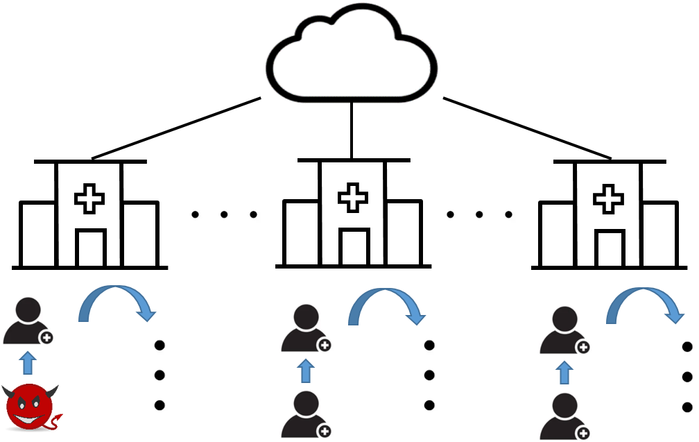
Figure 1: Our OFL architecture

Our OFL architecture is illustrated in Fig. 1. We have one server and $n$ learners, where each learner $i\in[n]$ interacts with streaming clients that arrive sequentially. We refer to the model parameters on the server and learners as the global model and local models, respectively. The learning task is for the server to coordinate all learners in training the global model online. The updated global model is then continuously released to the clients to provide instant service. To improve communication efficiency, learner $i$ utilizes the data of $\tau$ local clients to perform $\tau$ steps of local updates before sending the updated local model to the server. To formulate this intermittent communication, we define the entire time horizon as $\{0,1,\ldots,\tau-1,\ldots,(R-1)\tau,\ldots,R\tau-1\}$, with communication occurring at time step $\{r\tau:r\in[R]-1\}$, indicating a total of $R$ communication rounds spaced by $\tau$ intervals. At the $t$-th local update of the $r$-th communication round, the client, identified by $i^{r,t}\in[R\tau]$, queries the current global model $x^{r}$ and feeds back its data $D_{i}^{r,t}$ to learner $i$. The utility of the series of global models $\{x^{r}\}$ is quantified by a dynamic regret across the entire time horizon

$$\operatorname{Regret}_{d}:=\sum_{r=0}^{R-1}\sum_{t=0}^{\tau-1}\frac{1}{n}\sum_{i=1}^{n}(f_{i}^{r,t}(x^{r})-(f^{r})^{\star}).$$

Here, $f_{i}^{r,t}(x^{r})$ is the loss incurred by the global model $x^{r}$ on data $D_{i}^{r,t}$ and $(f^{r})^{\star}$ is a dynamic optimal loss defined by

$$(f^{r})^{\star}:=\min_{x}f^{r}(x):=\frac{1}{n\tau}\sum_{i=1}^{n}\sum_{t=0}^{\tau-1}f_{i}^{r,t}(x).$$

The word dynamic means the regret metric being a difference between the loss incurred by our online algorithm and a sequence of time-varying optimal losses. In contrast, another commonly used metric is called static regret defined by

$$\operatorname{Regret}_{s}:=\sum_{r=0}^{R-1}\sum_{t=0}^{\tau-1}\frac{1}{n}\sum_{i=1}^{n}(f_{i}^{r,t}(x^{r})-f^{r}(x^{\star})),$$

where $x^{\star}$ represents an optimal model, belonging to the optimal solution set $\mathcal{X}^{\star}$ that minimizes the cumulative loss over entire data, such that

$$x^{\star}\in\mathcal{X}^{\star}:=\underset{x}{\operatorname{argmin}}\sum_{r=0}^{R-1}\sum_{t=0}^{\tau-1}\frac{1}{n}\sum_{i=1}^{n}f_{i}^{r,t}(x).$$

Unlike $\operatorname{Regret}_{d}$, $\operatorname{Regret}_{s}$ compares against a static optimal loss, which is made by seeing all the data in advance. Note that the dynamic regret is more stringent and useful than the static one in practical OFL scenarios [24, 25].

In our paper, we aim to learn a series of $\{x^{r}\}$ that minimizes $\operatorname{Regret}_{d}$ while satisfying privacy constraints.

Privacy threat model: Considering the unique challenges of streaming data, we specifically allow a powerful adversary that can select data (cf. $D_{i}^{r,t}$) based on all previous outputs (cf. $\{x^{0},\ldots,x^{r}\}$), highlighting the adaptive nature of our threat model. Except this, our threat model is consistent with the central DP as known in the literatures [3, 26, 27], which relies on the server to add privacy preserving noise to the aggregated updates from learners. Both the server and all learners are trustworthy, while clients are semi-honest, meaning they execute the algorithm honestly but may attempt to infer the privacy of other clients through the released global model. Additionally, we assume that the communication channels between the server and the learners are secure, preventing clients from eavesdropping. We aim to guarantee clients’ privacy under the adaptive continuous release of global models $\{x_{1},\ldots,x_{R}\}$.

To quantify privacy leakage, we employ the concept of differential privacy. We define the aggregated dataset as $D=\{D_{i}^{r,t}:i\in[n],r\in[R]-1,t\in[\tau]-1\}$. DP is used over neighboring datasets $D$ and $D^{\prime}$ that differ by a single entry (for instance, replacing $D_{i}^{r,t}$ by ${D_{i}^{r,t}}^{\prime}$). The formal definition of DP is provided as follows [28].

Definition II.1

A randomized mechanism $\mathcal{M}$ satisfies $(\epsilon,\delta)$-DP if for any pair of neighboring datasets $D$ and $D^{\prime}$, and for any set of outcomes $O$ within the output domain,

$$\operatorname{Pr}[\mathcal{M}(D)\in{O}]\leq e^{\epsilon}\operatorname{Pr}\left[\mathcal{M}\left(D^{\prime}\right)\in{O}\right]+\delta.$$

Here, $\mathcal{M}(D)$ represents the whole sequence of outputs generated by the mechanism $\mathcal{M}$ throughout its execution, specifically $\{x_{1},\ldots,x_{R}\}$ in our OFL setting. The privacy protection level is quantified by two parameters, $\epsilon$ and $\delta$, where smaller values indicate stronger privacy protection.

III ALGORITHM

III-A Proposed algorithm

Algorithm 1 Proposed algorithm

1:Input: $R$, $\tau$, $\eta$, $\eta_{g}$, $\tilde{\eta}=\eta\eta_{g}\tau$, $x^{0}$, ${\bf B}$, $b^{0}=0$, and $(\epsilon,\delta)$-DP budget

2:Generate noise $\boldsymbol{\xi}\sim\mathcal{N}(0,V^{2})^{R\times d}$ where $V^{2}$ is determined to satisfy $(\epsilon,\delta)$-DP budget

3:for $r=0,1,\ldots,R-1$  do

4:     Learner $i$

5:     Set $z_{i}^{r,0}=x^{r}$

6:     for $t=0,1,\ldots,\tau-1$  do

7:         Respond with $x^{r}$ to the client $i^{r,t}$

8:         Obtain $D_{i}^{r,t}$ from client $i^{r,t}$

9:         Update $z_{i}^{r,t+1}=z_{i}^{r,t}-\eta\nabla f_{i}^{r,t}(z_{i}^{r,t})$

10:     end for

11:     Send $z_{i}^{r,\tau}$ to the server

12:     Server

13:     Update

$$x^{r+1}=x^{r}-\tilde{\eta}\left(\frac{1}{\eta\tau}\left(x^{r}-\frac{1}{n}\sum_{i=1}^{n}z_{i}^{r,\tau}\right)+(b^{r+1}-b^{r})\boldsymbol{\xi}\right)$$

14:end for

15:Output: $\{x^{1},\ldots,x^{R}\}$

We propose a DP algorithm for OFL, as outlined in Algorithm 1. The characteristic of our algorithm is the use of temporally correlated noise to protect privacy, alongside leveraging local updates to reduce the communication frequency between the server and learners.

Our algorithm consists of two loops: the outer loop is indexed by $r$ for communication rounds, and the inner loop is indexed by $t$ for local updates. At the $t$-th local update of the $r$-th communication round, learner $i$ responds with the current global model $x^{r}$ to the client $i^{r,t}$ and obtains the client data $D_{i}^{r,t}$. Learner $i$ then computes the gradient of the loss $f_{i}^{r,t}$ at $x^{r}$ using data $D_{i}^{r,t}$ and performs one step of local update with step size $\eta$. After $\tau$ local updates, the local model $z_{i}^{r,\tau}$ is sent to the server. The server averages these $z_{i}^{r,\tau},\forall i\in[n]$, updates the global model $x^{r}$ with step size $\tilde{\eta}$ and adds temporally correlated noise, specifically $(b^{r+1}-b^{r})\boldsymbol{\xi}$, to maintain the differential privacy of $x^{r+1}$.

To implement our algorithm, we need to construct the matrix ${\bf B}$ and determine the variance $V^{2}$ of DP noise. We will accomplish it via matrix factorization.

III-B Matrix factorization

Matrix factorization, originally developed for linear counting queries [22], has been adapted to enhance the privacy and utility for gradient-based algorithms [7]. This approach involves expressing the iterate of the gradient-based algorithm as $x^{r}=x^{0}-\tilde{\eta}\sum_{\tilde{r}=0}^{r-1}g_{\tilde{r}}$, where $g_{\tilde{r}}$ is the gradient-based direction at $\tilde{r}$-th iteration, thereby determining each $x^{r}$ by a cumulative sum that is a specific case of linear query release [7, Theorem B.1]. Therefore, the key DP primitive is accurately estimating cumulative sums over individual gradients. This principle pertains to the server-side update in our OFL. Indeed, we can equivalently reformulate Line 13 of Algorithm 1 as

$$x^{r+1}=x^{r}-\tilde{\eta}\left(g^{r}+(b^{r+1}-b^{r})\boldsymbol{\xi}\right),~{}\forall r\in[R]-1,$$ (1)

where $g^{r}=\frac{1}{n\tau}\sum_{t=0}^{\tau-1}\sum_{i=1}^{n}\nabla f_{i}^{r,t}(z_{i}^{r,t})$. Setting $b^{0}=0$ and repeated application of (1) result in

$${\bf x}={\bf x}^{0}-\tilde{\eta}({\bf A}{\bf G}+{\bf B}\boldsymbol{\xi}),$$ (2)

where $\mathbf{A}$ is a lower triangular matrix with 1s on and below the diagonal. Note that we do not require ${\bf B}$ to be lower-triangular because this requirement has been relaxed by utilizing the rotational invariance of the Gaussian distribution in [8, Proposition 2.2].

Although each entry of $\boldsymbol{\xi}$ is independent, the multiplication by matrix ${\bf B}$ introduces correlations among the rows of ${\bf B}\boldsymbol{\xi}$, complicating the privacy analysis. A strategic approach involves decomposing matrix ${\bf A}$ as ${\bf A}={\bf BC}$, thereby selecting such ${\bf B}$ to construct temporally correlated noise and then extracting ${\bf B}$ as a common factor. Substituting ${\bf{\bf A}}={\bf BC}$ into (2), we have

$${\bf x}={\bf x}^{0}-\tilde{\eta}{\bf B}({\bf C}{\bf G}+\boldsymbol{\xi}).$$ (3)

Here, the noise $\boldsymbol{\xi}$ with iid entries are added to ${\bf CG}$ and the privacy loss of (3) can be interpreted as the result of post-processing [29] following a single application of the Gaussian mechanism [8].

The determination of the suitable matrix factorization ${\bf B}{\bf C}$ and the variance $V^{2}$ of DP noise relies on the analysis of utility; hence, we will address this in the next section.

IV ANALYSIS

Throughout this paper, we impose the following assumptions on the loss functions.

Assumption IV.1

The loss function $f_{i}^{r,t}$ is $L$-smooth, i.e., for any $x,y$, there exists a constant $L$ such that

$$f_{i}^{r,t}(y)\leq f_{i}^{r,t}(x)+\langle\nabla f_{i}^{r,t}(x),y-x\rangle+\frac{L}{2}\|y-x\|^{2}.$$

Assumption IV.2

Consider the aggregated loss function $f^{r}$ and its optimal solution set $\mathcal{X}_{r}^{\star}:=\operatorname{argmin}_{x}f^{r}(x)$. The function $f^{r}$ is $\mu$-quasi strongly convex, i.e., for any $x$, there exists a constant $\mu$ such that

$$(f^{r})^{\star}\geq f^{r}(x)+\langle\nabla f^{r}(x),\operatorname{P}_{\mathcal{X}_{r}^{\star}}^{x}-x\rangle+\frac{\mu}{2}\|\operatorname{P}_{\mathcal{X}_{r}^{\star}}^{x}-x\|^{2}.$$

Assumption IV.3

Each loss function $f_{i}^{r,t}$ has bounded gradient, i.e., for any $x$, there exists a constant $B_{g}$ such that

$$\|\nabla f_{i}^{r,t}(x)\|\leq B_{g}.$$

Assumption IV.4

For any $x^{r}$, $x^{r}_{\xi}$, there exists a constant $\sigma$ such that $\|\operatorname{P}_{\mathcal{X}^{\star}}^{x^{r}}-\operatorname{P}_{\mathcal{X}^{\star}}^{x_{\xi}^{r}}\|\leq\sqrt{\sigma}\|x^{r}-x^{r}_{\xi}\|$.

Assumption IV.1 is standard in optimization literature. Assumptuon IV.2 is weaker than strong convexity and a function that is QSC may be non-convex, with specific examples seen in [30, 31]. Assumption IV.3 is frequently invoked in DP research to ensure bounded sensitivity [32, 33], and it aligns with the Lipschitz continuous condition of $f_{i}^{r,t}$ that is common in online learning literature [8, 1]. Assumption IV.4 is a regularity condition that is necessary for our analysis since $\mathcal{X}^{\star}$ for a QSC problem may not be convex.

With these assumptions, we are ready to establish the analysis of our algorithm on utility and privacy.

IV-A Utility

Inspired by the works [18, 34] in the single-machine setting, we employ the perturbed iterate analysis technique to control the impact of DP noise on utility. Observing the structure of temporally correlated noise $(b^{r+1}-b^{r})\boldsymbol{\xi}$, which is the difference of noises at successive communication rounds, we define a virtual variable $x^{r}_{\xi}$ as

$$x^{r}_{\xi}:=x^{r}+\tilde{\eta}b^{r}\boldsymbol{\xi},$$

and rewrite the update on the server (cf. Line 13 of Algorithm 1) as

$$x^{r+1}_{\xi}=x^{r}_{\xi}-\tilde{\eta}\cdot\frac{1}{\tau}\sum_{t=0}^{\tau-1}\frac{1}{n}\sum_{i=1}^{n}\nabla f_{i}^{r,t}(z_{i}^{r,t}),$$ (4)

where we substitute the fact that $\frac{1}{n}\sum_{i=1}^{n}z_{i}^{r,\tau}=x^{r}-\eta\sum_{t=0}^{\tau-1}\frac{1}{n}\sum_{i=1}^{n}\nabla f_{i}^{r,t}(z_{i}^{r,t})$ into Line 13 of Algorithm 1. Intuitively, the virtual variable $x^{r}_{\xi}$ is designed to subtract the DP noise in $x^{r}$, utilizing gradient information that remains untainted by DP noise for its update, as detailed (4). By analyzing the distance between $x^{r}_{\xi}$ and the optimal solution set $\mathcal{X}^{\star}$, we establish the following lemma regarding dynamic regret.

Lemma IV.5

Under Assumptions IV.1-IV.4, if $\tilde{\eta}\leq\frac{1}{8L}$, for Algorithm 1, we have

$$\frac{\operatorname{Regret}_{d}}{R\tau}\leq\frac{\mathbb{E}\|x_{\xi}^{0}-\operatorname{P}_{\mathcal{X}^{\star}}^{x_{\xi}^{0}}\|^{2}}{R\tilde{\eta}}+S^{r},$$

where

$$S^{r}:=\left(\tilde{\eta}+\frac{1}{12L}+\frac{1}{\mu}\right)2L^{2}\frac{\tilde{\eta}^{2}}{\eta_{g}^{2}}B_{g}^{2}$$

$$+\frac{24L(1+\sigma)\tilde{\eta}^{2}}{R}\|{\bf B}\|_{F}^{2}dV^{2}+\frac{\left(12L+{\mu}\right)C_{R}}{R}$$

and $C_{R}:=\sum_{r=0}^{R-1}\mathbb{E}\|\operatorname{P}_{\mathcal{X}_{r}^{\star}}^{x^{r}}-\operatorname{P}_{\mathcal{X}^{\star}}^{x^{r}}\|^{2}$.

As shown in Lemma IV.5, the term $S^{r}$ encapsulates several distinct sources of error including the term $B_{g}$ caused by the drift error from local updates, the term $V^{2}$ caused by DP noise, and the term $C_{R}$ caused by the dynamic environment.

IV-B Privacy

Recall that ${\bf A}={\bf BC}$ and the equivalence of Algorithm 1 to ${\bf x}={\bf x}^{0}-\tilde{\eta}{\bf B}({\bf C}{\bf G}+\boldsymbol{\xi})$. Lemma IV.5 illuminates the impact of ${\bf B}$ and $V^{2}$ on utility. It is equally crucial to know the influence of ${\bf B}$, ${\bf C}$, and $V^{2}$ on privacy loss to determine their values. Based on our privacy threat model and the definition of neighboring data sets in Section II, we can adopt the methodology from the single-machine setting [8] to analyze the privacy loss incurred by the adaptive continuous release of $\{x^{1},\ldots,x^{R}\}$.

Theorem IV.6 (Theorems 2.1 and 3.1 in [8])

Consider a lower-triangular matrix $\mathbf{A}$ of full rank and its factorization $\mathbf{A}=\mathbf{BC}$. For any neighboring sets $\mathbf{G},\mathbf{G}^{\prime}\in\mathbb{R}^{R\times d}$, it holds that $\|\mathbf{C}(\mathbf{G}-\mathbf{G}^{\prime})\|_{F}\leq 2\gamma B_{g}$ where $\gamma=\max_{r\in[R]}\|\mathbf{C}_{[:,r]}\|$ is the largest column norm of $\mathbf{C}$. Given the Gaussian noise $\boldsymbol{\xi}\sim\mathcal{N}\left(0,\frac{4\gamma^{2}B_{g}^{2}(2\log(1/\delta)+\epsilon)}{\epsilon^{2}}\right)^{R\times d}$, if the mechanism $\mathcal{M}(\mathbf{G})=\mathbf{B}(\mathbf{CG}+\boldsymbol{\xi})$ satisfies $(\varepsilon,\delta)$-DP in the nonadaptive continuous release, then $\mathcal{M}$ satisfies the same DP guarantee with the same parameters even when the rows of ${\bf G}$ are chosen adaptively.

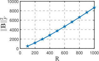
Figure 2: Test to show the validity of $\|{\bf B}\|_{F}^{2}=\mathcal{O}(R^{2})$

To achieve higher accuracy, Theorem IV.6 suggests a small $\gamma=\max_{r\in[R]}\|\mathbf{C}_{[:,r]}\|$ and Lemma IV.5 suggests a small $\|{\bf B}\|^{2}_{F}$. Let us define $\mathbf{C}^{\dagger}$ as the Moore-Penrose pseudo-inverse of ${\bf C}$. Under the fact that $\mathbf{A}\mathbf{C}^{\dagger}$ yields the minimal $\ell_{2}$-norm solution for solving the linear equation ${\bf A}={\bf BC}$, the work [8] proposes to construct the matrix factors ${\bf B}$ and ${\bf C}$ through the optimization problem

$$\min_{\mathbf{C}\in\mathbf{V},\gamma^{2}(\mathbf{C})=1}\|\mathbf{A}\mathbf{C}^{\dagger}\|_{F}^{2},$$ (5)

where $\mathbf{V}$ is a linear space of matrices. The closed-form solution of (5) can be found in [8, Theorem 3.2].

By using (5), we can guarantee that $\gamma=1$. For $\|{\bf B}\|_{F}^{2}$, we assume that $\|{\bf B}\|_{F}^{2}=\mathcal{O}(R^{2})$ by observing that there are $R^{2}$ entries in ${\bf B}$, each of which are bounded. To show that $\|{\bf B}\|_{F}^{2}=\mathcal{O}(R^{2})$ is reasonable (even overly conservative), we run the algorithm for solving (5) in [8, Theorem 3.2] and plot $\|{\bf B}\|_{F}^{2}$ versus $R$ in Fig. 2, which shows that $\|{\bf B}\|_{F}^{2}$ is much smaller than $R^{2}$. Note that the factorization only requires prior knowledge of $R$, and it is calculated offline only once before the algorithm starts running.

IV-C Utility-privacy

Combining Lemma IV.5, Theorem IV.6, and $\|{\bf B}\|_{F}^{2}=\mathcal{O}(R^{2})$, we get the utility-privacy trade-off.

Theorem IV.7

Under Assumptions IV.1-IV.4, if $\tilde{\eta}\leq\frac{1}{8L}$ and $\tilde{\eta}=\mathcal{O}(1/R^{\frac{2}{3}})$, Algorithm 1 subject to $(\epsilon,\delta)$-DP satisfies

$$\frac{\operatorname{Regret}_{d}}{R\tau}\leq \mathcal{O}\left(\frac{\mathbb{E}\|x_{\xi}^{0}-\operatorname{P}_{\mathcal{X}^{\star}}^{x_{\xi}^{0}}\|^{2}}{R^{\frac{1}{3}}}+\frac{B_{g}^{2}}{\eta_{g}^{2}R^{\frac{4}{3}}}\right.$$

$$\left.+\frac{d}{R^{\frac{1}{3}}}\frac{B_{g}^{2}(\log(1/\delta)+\epsilon)}{\epsilon^{2}}+\frac{C_{R}}{R}\right).$$

In Theorem IV.7, the errors are due to the initial error, the local updates, the DP noise, and the dynamic environment, respectively. We have the following observations.

• Given that $\tilde{\eta}=\eta\eta_{g}\tau$ and $\tilde{\eta}<\frac{1}{8L}$, the number of local updates $\tau$ cannot be excessively large. Such a choice would necessitate a smaller $\eta_{g}$, leading to a larger $\frac{B_{g}^{2}}{\eta_{g}^{2}R^{\frac{4}{3}}}$.

• Our perturbed iterate analysis well-controls the impact of DP noise on utility. This is reflected in the error term caused by DP noise being $\mathcal{O}(1/R^{\frac{1}{3}})$, which decreases as $R$ increases.

• The term $C_{R}:=\sum_{r=0}^{R-1}\mathbb{E}\|\operatorname{P}_{\mathcal{X}_{r}^{\star}}^{x^{r}}-\operatorname{P}_{\mathcal{X}^{\star}}^{x^{r}}\|^{2}$ captures that the solution set $\mathcal{X}_{r}^{\star}$ changes over time relative to a fixed solution set $\mathcal{X}^{\star}$, which is unavoidable for dynamic regret [35, Theorem 5]. Intuitively, when the environment changes very rapidly, online learning algorithms struggle to achieve high utility. On the other hand, establishing a sub-linear regret bound for non-convex problems, even for static regret, presents significant challenges [24, Proposition 1]. Thus, to remove the dependence on $C_{R}$, we establish a sub-linear static regret bound under SC, where SC simplifies the analysis by allowing us to follow steps similar to those in QSC.

Corollary IV.8 (Static regret under SC)

Assume the loss function $f^{r}$ to be strongly convex, i.e., there exists a constant $\mu$ such that

$$f^{r}(x)-f^{r}(x^{\star})+\frac{\mu}{2}\|x-x^{\star}\|^{2}\leq\left\langle\nabla f^{r}(x),x-x^{\star}\right\rangle,~{}\forall x,$$

where $x^{\star}:=\operatorname{argmin}_{x}\sum_{r=0}^{R-1}f^{r}(x)$. Then under Assumpitions IV.1, IV.3 and IV.4, if $\tilde{\eta}\leq\frac{1}{10LR^{\frac{1}{2}}}$ and $\tilde{\eta}=\mathcal{O}(1/R^{\frac{3}{4}})$, Algorithm 1 subject to $(\epsilon,\delta)$-DP satisfies

$$\frac{\operatorname{Regret}_{s}}{R\tau}\leq \mathcal{O}\left(\frac{\mathbb{E}\|x_{\xi}^{0}-x^{\star}\|^{2}}{R^{\frac{1}{4}}}+\frac{B_{g}^{2}}{\eta_{g}^{2}R^{\frac{3}{2}}}\right.$$

$$\left.+\frac{d}{R^{\frac{1}{4}}}\frac{B_{g}^{2}(\log(1/\delta)+\epsilon)}{\epsilon^{2}}+\frac{C_{R}}{R^{\frac{5}{4}}}\right),$$

where $C_{R}:=\sum_{r=0}^{R-1}\|x^{\star}-x_{r}^{\star}\|^{2}$ and $x_{r}^{\star}:=\operatorname{argmin}_{x}f^{r}(x)$.

In Corrolary IV.8, the error term caused by $C_{R}$ converges at the rate of $\mathcal{O}(1/R^{\frac{5}{4}})$ for a static regret under SC.

Remark IV.9

We compare our results with two closely related state-of-the-art approaches [1] and [8].

The work [1] uses local updates with non-iid streaming data for OFL but for convex problems without DP protection. The regret in [1] is static and defined on the local models, i.e., $\operatorname{Regret}_{s}^{\operatorname{local}}:=\sum_{r=0}^{R-1}\sum_{t=0}^{\tau-1}\frac{1}{n}\sum_{i=1}^{n}(f_{i}^{r,t}(z_{i}^{r,t})-f^{r}(x^{\star}))$, while ours is dynamic or static and is defined on the released global model $x^{r}$. The regret in [1] is upper bounded by $\mathcal{O}(\tau\log(\tau R))$ for SC case and $\mathcal{O}(\tau R^{\frac{1}{2}})$ for convex case, while our $\operatorname{Regret}_{s}$ is bounded by $\mathcal{O}(\tau R^{\frac{3}{4}})$ for SC case and our $\operatorname{Regret}_{d}$ is bounded by $\mathcal{O}(\tau R^{\frac{2}{3}}+\tau C_{R})$ for QSC case.

The work [8] uses MF to guarantee DP for online learning under the adaptive continuous release but for convex problems in the single-machine setting. The regret in [8, Proposition 4.1] is static and satisfies

$$\frac{\operatorname{Regret}_{s}^{\operatorname{single}}}{R}\leq\mathcal{O}\left(\frac{E^{0}}{R\eta}+\frac{\eta\|\mathbf{B}\|_{F}}{\sqrt{R}}B_{g}V+\eta B_{g}^{2}\right)$$ (6)

$$\leq\mathcal{O}\left(\frac{E^{0}}{R\eta}+{\eta\sqrt{R}}B_{g}^{2}\sqrt{\frac{(\log(1/\delta)+\epsilon)}{\epsilon^{2}}}+\eta B_{g}^{2}\right),$$

where $E^{0}$ is a constant about initial error and we substitute $\|{\bf B}\|_{F}=\mathcal{O}(R)$, $\gamma=1$, and $V=\sqrt{\frac{4B_{g}^{2}(2\log(1/\delta)+\epsilon)}{\epsilon^{2}}}$ in the second inequality. To draw a comparison with our findings, we select the step size $\eta$ in (6). By setting $\mathcal{O}\left(\frac{1}{R\eta}\right)=\mathcal{O}(\eta\sqrt{R})$, $\operatorname{Regret}_{s}^{\operatorname{single}}$ in [8] becomes

$$\frac{\operatorname{Regret}_{s}^{\operatorname{single}}}{R}\leq\mathcal{O}\left(\frac{E^{0}}{R^{\frac{1}{4}}}+\frac{B_{g}^{2}}{R^{\frac{1}{4}}}\sqrt{\frac{(\log(1/\delta)+\epsilon)}{\epsilon^{2}}}+\frac{B_{g}^{2}}{R^{\frac{3}{4}}}\right),$$

which implies that $\operatorname{Regret}_{s}^{\operatorname{single}}$ in [8] is bounded by $\mathcal{O}\left(R^{\frac{3}{4}}\sqrt{\frac{(\log(1/\delta)+\epsilon)}{\epsilon^{2}}}\right)$. Adapting our algorithm for $n=1$, $\tau=1$, and $\eta_{g}=1$, it reduces to a single-machine algorithm. Our $\operatorname{Regret}_{s}$ is bounded by $\mathcal{O}\left(R^{\frac{3}{4}}\frac{(\log(1/\delta)+\epsilon)}{\epsilon^{2}}\right)$ for SC case and our $\operatorname{Regret}_{d}$ is bounded by $\mathcal{O}\left(R^{\frac{2}{3}}\frac{(\log(1/\delta)+\epsilon)}{\epsilon^{2}}+C_{R}\right)$ for QSC case. Additionally, our proof uses QSC or SC while algorithm in [8] uses general convexity, which accounts for the different dependency on $\epsilon$; ours is $(\log(1/\delta)+\epsilon)/\epsilon^{2}$ while that in [8] is $\sqrt{(\log(1/\delta)+\epsilon)/\epsilon^{2}}$.

V EXPERIMENTS

Consider a logistic regression problem

$$\underset{{x}}{\operatorname{min}}\;\frac{1}{R\tau n}\sum_{r=0}^{R-1}\sum_{t=0}^{\tau-1}\sum_{i=1}^{n}f_{i}^{r,t}(x),$$

where $f_{i}^{r,t}(x)=\log\left(1+\exp\left(-\left({x}\mathbf{a}_{i}^{r,t}\right)b_{i}^{r,t}\right)\right)$ is the loss function on learner $i$ and $(\mathbf{a}_{i}^{r,t},b_{i}^{r,t})\in\mathbb{R}^{d}\times\{-1,+1\}$ is the feature-label pair. To generate data, we use the method in [36] which allows us to control the degree of heterogeneity by two parameters $(\alpha,\beta)$. The experiments are carried out 20 times, with the results being averaged and displayed along with error bars to indicate the standard deviation.

V-1 Impact of $\tau$

In the first set of experiments, we show the impact of $\tau$ on our algorithm. We set $n=10$ learners, with each learner receiving $800$ streaming clients. We set the parameters on data heterogeneity to $(\alpha,\beta)=(0.1,0.1)$ and the privacy budget to $(5,1e^{-3})$-DP. We set $\tau\in\{1,2,4\}$, with corresponding $R\in\{800,400,200\}$, so that the total data used in each test is the same. The step-sizes are the same in all tests. The results are shown in Fig. 3. The $y$-axis represents $\operatorname{loss~{}error}$ of the current $x^{r}$ over the entire dataset,

$$\operatorname{loss~{}error}=\frac{1}{R\tau n}\sum_{\tilde{r}=0}^{R-1}\sum_{t=0}^{\tau-1}\sum_{i=1}^{n}(f_{i}^{\tilde{r},t}(x^{r})-f_{i}^{\tilde{r},t}(x^{\star}))$$

and the $x$-axis represents the communication round. Our algorithm achieves almost the same utility with fewer communications as $\tau$ increases while satisfying $(5,1e^{-3})$-DP.

V-2 Comparison under different DP budgets

We are unaware of any algorithm that considers the same setting as we do. The closest work appears to be the differentially private OFL algorithm in [3]. However, in contrast to us, their algorithm uses independent DP noise and does not consider the adaptive continuous release. Its server-side update is

$$x^{r+1}=x^{r}-\eta\left(\frac{1}{n}\sum_{i=1}^{n}\sum_{t=0}^{\tau-1}\nabla f_{i}^{r,t}(x^{r})+\zeta\right),$$ (7)

where $\zeta\sim{\mathcal{N}}(0,V^{2})^{1\times d}$. The work in [3] is compelling since $V^{2}$ required to satisfy the privacy budget can be chosen independently of $R$ and $\tau$. Specifically, according to [3], using the neighboring definition of streaming data, the variance in (7) is set as $V^{2}={2B_{g}^{2}}/{\rho}$ with $\rho=\left(\sqrt{\epsilon+\log{1}/{\delta}}-\sqrt{\log{1}/{\delta}}\right)^{2}\approx\frac{\epsilon^{2}}{4\log\frac{1}{\delta}}$ to ensure (7) is $\rho$-zCDP [37] and equivalently is $(\epsilon,\delta)$-DP after releasing $\{x^{1},\ldots,x^{R}\}$.

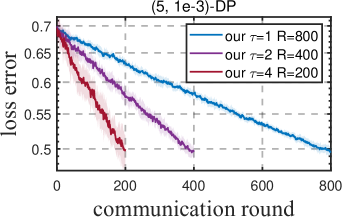
Figure 3: Impact of $\tau$

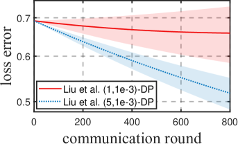
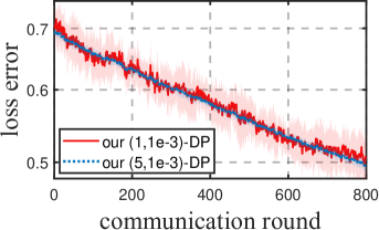
Figure 4: Comparison under different DP budgets

In the second set of experiments, we set $n=10$ learners, with each learner managing 8000 clients step by step, where $\tau=10$ and $R=800$, respectively. We set $(\alpha,\beta)=(0.1,0.1)$. We compare our algorithm with [3] under two privacy budgets $(\epsilon,\delta)\in\{(5,1e^{-3}),(1,1e^{-3})\}$.

The results are shown in Fig. 4. For our algorithm, we use the same step sizes under both privacy budgets, allowing our algorithm to maintain almost the same convergence rate, although the variance of the results increases when the privacy budget is stricter (i.e., $(1,1e^{-3})$-DP). For the compared algorithm, the variance also increases as the privacy requirements become more stringent, but in addition, the algorithm has to use a smaller step-size and the convergence slows down by a lot. Our algorithm performs better than [3], thanks to the use of correlated noise which allows to reduce the amount of perturbation on the utility.

VI CONCLUSIONS

We have proposed a DP algorithm for OFL which uses temporally correlated noise to protect client privacy under adaptive continuous release. To overcome the challenges caused by DP noise and local updates with streaming non-iid data, we use a perturbed iterate analysis to control the impact of the DP noise on the utility. Moreover, we show how the drift error from local updates can be managed under a QSC condition. Subject to a fixed DP budget, we establish a dynamic regret bound that explicitly shows the trade-off between utility and privacy. Numerical results demonstrate the efficiency of our algorithm. Future research directions include extending the temporally correlated noise to scenarios where the server is not trusted, designing optimal matrix factorization strategies tailored to improve utility, and exploring the application of the proposed algorithms to real-world scenarios in online control and signal processing.

Appendix A Fixed step size $\tilde{\eta}$

The local and global updates of the proposed Algorithm 1 can be expressed as

$$z_{i}^{r,t+1} =z_{i}^{r,t}-\eta{\nabla f_{i}^{r,t}}(z_{i}^{r,t}),~{}\forall t\in[\tau]-1,r\in[R]-1,$$ (8)

$$x^{r+1} =x^{r}-\tilde{\eta}\left(\frac{1}{n\tau}\sum_{t=0}^{\tau-1}\sum_{i=1}^{n}\nabla f_{i}^{r,t}(z_{i}^{r,t})+(b^{r+1}-b^{r})\boldsymbol{\xi}\right),$$

where $z_{i}^{r,0}=x^{r}$, $\tilde{\eta}=\eta_{g}\eta\tau$, $\boldsymbol{\xi}\sim\mathcal{N}(0,V^{2})^{R\times d}$.

We aim to achieve tighter convergence by utilizing the structure of temporally correlated noise. To this end, we define

$$x^{r}_{\xi}:=x^{r}+\tilde{\eta}b^{r}\boldsymbol{\xi}$$

and then the global updates in (8) yields

$$x^{r+1}_{\xi}=x^{r}_{\xi}-\tilde{\eta}\underbrace{\frac{1}{\tau}\sum_{t=0}^{\tau-1}\frac{1}{n}\sum_{i=1}^{n}\nabla f_{i}^{r,t}(z_{i}^{r,t})}_{:=g^{r}}.$$ (9)

In the following analysis, we focus on the sequence $\{x^{r}_{\xi}\}_{r}$ instead of $\{x^{r}\}_{r}$.

A-A QSC case: proof of Lemma IV.5

With (9), we have

$$\mathbb{E}\|x_{\xi}^{r+1}-\operatorname{P}_{\mathcal{X}^{\star}}^{x_{\xi}^{r+1}}\|^{2}$$ (10)

$$\leq \mathbb{E}\|x_{\xi}^{r}-\operatorname{P}_{\mathcal{X}^{\star}}^{x_{\xi}^{r}}-\tilde{\eta}g^{r}\|^{2}$$

$$= \mathbb{E}\|x_{\xi}^{r}-\operatorname{P}_{\mathcal{X}^{\star}}^{x_{\xi}^{r}}\|^{2}+{\tilde{\eta}^{2}\mathbb{E}\|g^{r}\|^{2}}$$

$${-2\tilde{\eta}\mathbb{E}\left\langle g^{r},x_{\xi}^{r}-x^{r}+x^{r}-\operatorname{P}_{\mathcal{X}^{\star}}^{x^{r}}+\operatorname{P}_{\mathcal{X}^{\star}}^{x^{r}}-\operatorname{P}_{\mathcal{X}^{\star}}^{x_{\xi}^{r}}\right\rangle}$$

$$\leq \mathbb{E}\|x_{\xi}^{r}-\operatorname{P}_{\mathcal{X}^{\star}}^{x_{\xi}^{r}}\|^{2}\underbrace{-2\tilde{\eta}\mathbb{E}\left\langle g^{r},x^{r}-\operatorname{P}_{\mathcal{X}^{\star}}^{x^{r}}\right\rangle}_{\rm(IV)}+\tilde{\eta}^{2}\left(1+\frac{\theta}{\tilde{\eta}}\right)\underbrace{\mathbb{E}\|g^{r}\|^{2}}_{\rm(V)}$$

$$+\frac{2\tilde{\eta}}{\theta}\left(\mathbb{E}\|x_{\xi}^{r}-x^{r}\|^{2}+\mathbb{E}\|\operatorname{P}_{\mathcal{X}^{\star}}^{x^{r}}-\operatorname{P}_{\mathcal{X}^{\star}}^{x_{\xi}^{r}}\|^{2}\right),$$

where the first inequality is from the optimality of $\operatorname{P}_{\mathcal{X}^{\star}}^{x_{\xi}^{r+1}}$ and the second inequality is from $2a^{T}b\leq\theta\|a\|^{2}+\frac{1}{\theta}\|b\|^{2}$ for any $\theta>0$. To bound the term (IV), adding and subtracting $\nabla f_{i}^{r,t}(x^{r})$ yields

$${\rm(IV)}=-2\tilde{\eta}\mathbb{E}\left\langle\frac{1}{n\tau}\sum_{t=0}^{\tau-1}\sum_{i=1}^{n}\nabla f_{i}^{r,t}(x^{r}),x^{r}-\operatorname{P}_{\mathcal{X}^{\star}}^{x^{r}}\right\rangle$$

$$-2\tilde{\eta}\mathbb{E}\left\langle\frac{1}{n\tau}\sum_{t=0}^{\tau-1}\sum_{i=1}^{n}(\nabla f_{i}^{r,t}(z_{i}^{r,t})-\nabla f_{i}^{r,t}(x^{r})),x^{r}-\operatorname{P}_{\mathcal{X}^{\star}}^{x^{r}}\right\rangle.$$

We define the two terms on the right hand of the above equality as (IV.I) and (IV.II), respectively. For (IV.I), we use the QSC to get that the cross term yields descent with the quantity

$${\rm(IV.I)}$$

$$= -2\tilde{\eta}\mathbb{E}\left\langle\frac{1}{n\tau}\sum_{t=0}^{\tau-1}\sum_{i=1}^{n}\nabla f_{i}^{r,t}(x^{r}),x^{r}-\operatorname{P}_{\mathcal{X}_{r}^{\star}}^{x^{r}}+\operatorname{P}_{\mathcal{X}_{r}^{\star}}^{x^{r}}-\operatorname{P}_{\mathcal{X}^{\star}}^{x^{r}}\right\rangle$$

$$\leq -\frac{2\tilde{\eta}}{n\tau}\sum_{i=1}^{n}\sum_{t=0}^{\tau-1}\mathbb{E}(f_{i}^{r,t}(x^{r})-(f^{r})^{\star})-{\tilde{\eta}\mu}\mathbb{E}\|x^{r}-\operatorname{P}_{\mathcal{X}_{r}^{\star}}^{x^{r}}\|^{2}$$

$$+\tilde{\eta}\left(\theta\mathbb{E}\left\|\frac{1}{n\tau}\sum_{i=1}^{n}\sum_{t=0}^{\tau-1}\nabla f_{i}^{r,t}(x^{r})\right\|^{2}+\frac{1}{\theta}\mathbb{E}\|\operatorname{P}_{\mathcal{X}_{r}^{\star}}^{x^{r}}-\operatorname{P}_{\mathcal{X}^{\star}}^{x^{r}}\|^{2}\right),$$

where for the inequality we also use $2a^{T}b\leq\theta\|a\|^{2}+\frac{1}{\theta}\|b\|^{2}$ for any $\theta>0$ and Assumption IV.2 such that

$$\frac{1}{n\tau}\sum_{i=1}^{n}\sum_{t=0}^{\tau-1}(f_{i}^{r,t}(x)-(f^{r})^{\star})+\frac{\mu}{2}\|x-\operatorname{P}_{\mathcal{X}_{r}^{\star}}^{x}\|^{2}$$

$$\leq \left\langle\frac{1}{n\tau}\sum_{i=1}^{n}\sum_{t=0}^{\tau-1}\nabla f_{i}^{r,t}(x),x-\operatorname{P}_{\mathcal{X}_{r}^{\star}}^{x}\right\rangle,~{}\forall x.$$

For the term (IV.II), observing that after using triangle inequality we have

$${\rm(IV.II)}$$

$$= -2\tilde{\eta}\mathbb{E}\left\langle\frac{1}{n\tau}\sum_{t=0}^{\tau-1}\sum_{i=1}^{n}(\nabla f_{i}^{r,t}(z_{i}^{r,t})-\nabla f_{i}^{r,t}(x^{r})),x^{r}-\operatorname{P}_{\mathcal{X}^{\star}}^{x^{r}}\right\rangle$$

$$\leq \frac{2\tilde{\eta}}{\mu}\mathbb{E}\left\|\frac{1}{n\tau}\sum_{t=0}^{\tau-1}\sum_{i=1}^{n}(\nabla f_{i}^{r,t}(z_{i}^{r,t})-\nabla f_{i}^{r,t}(x^{r}))\right\|^{2}$$

$$+\tilde{\eta}\mu\left(\mathbb{E}\|x^{r}-\operatorname{P}_{\mathcal{X}_{r}^{\star}}^{x^{r}}\|^{2}+\|\operatorname{P}_{\mathcal{X}_{r}^{\star}}^{x^{r}}-\operatorname{P}_{\mathcal{X}^{\star}}^{x^{r}}\|^{2}\right).$$

Substituting (IV.I) and (IV.II) into (IV), it follows that

$${\rm(IV)}\leq -\frac{2\tilde{\eta}}{n\tau}\sum_{i=1}^{n}\sum_{t=0}^{\tau-1}\mathbb{E}(f_{i}^{r,t}(x^{r})-(f^{r})^{\star})$$

$$+\tilde{\eta}\theta\mathbb{E}\left\|\frac{1}{n\tau}\sum_{i=1}^{n}\sum_{t=0}^{\tau-1}\nabla f_{i}^{r,t}(x^{r})\right\|^{2}$$

$$+\tilde{\eta}\left(\frac{1}{\theta}+\mu\right)\mathbb{E}\|\operatorname{P}_{\mathcal{X}_{r}^{\star}}^{x^{r}}-\operatorname{P}_{\mathcal{X}^{\star}}^{x^{r}}\|^{2}$$

$$+\frac{2\tilde{\eta}}{\mu}\mathbb{E}\left\|\frac{1}{n\tau}\sum_{t=0}^{\tau-1}\sum_{i=1}^{n}(\nabla f_{i}^{r,t}(z_{i}^{r,t})-\nabla f_{i}^{r,t}(x^{r}))\right\|^{2}.$$

Next, for the term (V) in (10), adding and subtracting $\nabla f_{i}^{r,t}(x^{r})$, we have

$${\rm(V)}$$

$$= \mathbb{E}\left\|\frac{1}{n\tau}\sum_{i=1}^{n}\sum_{t=0}^{\tau-1}(\nabla f_{i}^{r,t}(z_{i}^{r,t})-\nabla f_{i}^{r,t}(x^{r})+\nabla f_{i}^{r,t}(x^{r}))\right\|^{2}$$

$$\leq 2\mathbb{E}\left\|\frac{1}{n\tau}\sum_{i=1}^{n}\sum_{t=0}^{\tau-1}(\nabla f_{i}^{r,t}(z_{i}^{r,t})-\nabla f_{i}^{r,t}(x^{r}))\right\|^{2}$$

$$+2\mathbb{E}\left\|\frac{1}{n\tau}\sum_{i=1}^{n}\sum_{t=0}^{\tau-1}\nabla f_{i}^{r,t}(x^{r})\right\|^{2}.$$

Substituting (IV) and (V) into (10), we have

$$\mathbb{E}\|x_{\xi}^{r+1}-\operatorname{P}_{\mathcal{X}^{\star}}^{x_{\xi}^{r+1}}\|^{2}-\mathbb{E}\|x_{\xi}^{r}-\operatorname{P}_{\mathcal{X}^{\star}}^{x_{\xi}^{r}}\|^{2}$$ (11)

$$\leq-\frac{2\tilde{\eta}}{n\tau}\sum_{i=1}^{n}\sum_{t=0}^{\tau-1}\mathbb{E}(f_{i}^{r,t}(x^{r})-(f^{r})^{\star})$$

$$+2c_{{\rm VI}}\cdot\underbrace{\mathbb{E}\Big{\|}\frac{1}{n\tau}\sum_{i=1}^{n}\sum_{t=0}^{\tau-1}(\nabla f_{i}^{r,t}(z_{i}^{r,t})-\nabla f_{i}^{r,t}(x^{r}))\Big{\|}^{2}}_{\rm(VI)}$$

$$+2c_{{\rm VII}}\cdot\underbrace{\mathbb{E}\left\|\frac{1}{n\tau}\sum_{i=1}^{n}\sum_{t=0}^{\tau-1}\nabla f_{i}^{r,t}(x^{r})\right\|^{2}}_{\rm(VII)}$$

$$+\frac{2\tilde{\eta}}{\theta}\left(\mathbb{E}\|x_{\xi}^{r}-x^{r}\|^{2}+\mathbb{E}\|\operatorname{P}_{\mathcal{X}^{\star}}^{x^{r}}-\operatorname{P}_{\mathcal{X}^{\star}}^{x_{\xi}^{r}}\|^{2}\right)$$

$$+\tilde{\eta}\left(\frac{1}{\theta}+\mu\right)\mathbb{E}\|\operatorname{P}_{\mathcal{X}_{r}^{\star}}^{x^{r}}-\operatorname{P}_{\mathcal{X}^{\star}}^{x^{r}}\|^{2},$$

where $c_{{\rm VI}}:=\tilde{\eta}^{2}\left(1+\frac{\theta}{\tilde{\eta}}\right)+\frac{\tilde{\eta}}{\mu}$ and $c_{{\rm VII}}:=\tilde{\eta}^{2}\left(1+\frac{3\theta}{2\tilde{\eta}}\right)$.

For the term (VI), we can transfer it to the drift error that

$${\rm(VI)}\leq L^{2}\frac{1}{n\tau}\sum_{i=1}^{n}\sum_{t=0}^{\tau-1}\mathbb{E}\|z_{i}^{r,t}-x^{r}\|^{2}$$

by repeatedly applying the local updates $z_{i}^{r,\tau-1}=z_{i}^{r,1}-\eta\sum_{t=1}^{\tau-1}\nabla f_{i}^{r,t}(z_{i}^{r,t})$ and $z_{i}^{r,0}=x^{r}$. From $\|\nabla f_{i}^{r,t}(x)\|\leq B_{g}$ for any $x$, we have

$$\|z_{i}^{r,\tau-1}-x^{r}\|^{2}=\left\|\eta\sum_{t=0}^{\tau-1}\nabla f_{i}^{r,t}(z_{i}^{r,t})\right\|^{2}\leq\eta^{2}\tau^{2}B_{g}^{2}.$$ (12)

Substituting (12) into (VI), we have

$${\rm(VI)}\leq L^{2}\eta^{2}\tau^{2}B_{g}^{2}.$$

To handle the term (VII), we use the $L$-smoothness to transfer the gradient norm to the loss value. To this end, we use the following fact

$$f_{i}^{r,t}(y)\leq f_{i}^{r,t}(x)+\langle\nabla f_{i}^{r,t}(x),y-x\rangle+\frac{L}{2}\|y-x\|^{2}.$$

Optimizing both hands of above inequality w.r.t. $y$, we get

$$(f^{r})^{\star}\leq\min_{y}\frac{1}{n\tau}\sum_{i=1}^{n}\sum_{t=0}^{\tau-1}f_{i}^{r,t}(y)$$

$$\leq \frac{1}{n\tau}\sum_{i=1}^{n}\sum_{t=0}^{\tau-1}f_{i}^{r,t}(x)-\frac{1}{2L}\left\|\frac{1}{n\tau}\sum_{i=1}^{n}\sum_{t=0}^{\tau-1}\nabla f_{i}^{r,t}(x)\right\|^{2}$$

$$+\frac{L}{2}\min_{y}\left\{\left\|y-\left(x-\frac{1}{n\tau L}\sum_{i=1}^{n}\sum_{t=0}^{\tau-1}\nabla f_{i}^{r,t}(x)\right)\right\|^{2}\right\}$$

$$= \frac{1}{n\tau}\sum_{i=1}^{n}\sum_{t=0}^{\tau-1}f_{i}^{r,t}(x)-\frac{1}{2L}\left\|\frac{1}{n\tau}\sum_{i=1}^{n}\sum_{t=0}^{\tau-1}\nabla f_{i}^{r,t}(x)\right\|^{2},$$

which implies that

$$\left\|\frac{1}{n\tau}\sum_{i=1}^{n}\sum_{t=0}^{\tau-1}\nabla f_{i}^{r,t}(x)\right\|^{2}\leq 2L\left(\frac{1}{n\tau}\sum_{i=1}^{n}\sum_{t=0}^{\tau-1}f_{i}^{r,t}(x)-(f^{r})^{\star}\right).$$ (13)

Substituting (13) into (VII), we have

$${\rm(VII)} =\mathbb{E}\left\|\frac{1}{n\tau}\sum_{i=1}^{n}\sum_{t=0}^{\tau-1}\nabla f_{i}^{r,t}(x^{r})\right\|^{2}$$

$$\leq\frac{1}{n\tau}\sum_{i=1}^{n}\sum_{t=0}^{\tau-1}2L\mathbb{E}(f_{i}^{r,t}(x^{r})-(f^{r})^{\star}).$$

From the derived upper bounds for (VI) and (VII) with (11), it follows that

$$\mathbb{E}\|x_{\xi}^{r+1}-\operatorname{P}_{\mathcal{X}^{\star}}^{x_{\xi}^{r+1}}\|^{2}-\mathbb{E}\|x_{\xi}^{r}-\operatorname{P}_{\mathcal{X}^{\star}}^{x_{\xi}^{r}}\|^{2}$$

$$\leq\underbrace{-\left({2\tilde{\eta}}-\tilde{\eta}^{2}\left(1+\frac{3\theta}{2\tilde{\eta}}\right)4L\right)}_{\leq-\tilde{\eta}}\frac{1}{n\tau}\sum_{i=1}^{n}\sum_{t=0}^{\tau-1}\mathbb{E}(f_{i}^{r,t}(x^{r})-(f^{r})^{\star})$$

$$+\left(\tilde{\eta}^{2}\left(1+\frac{\theta}{\tilde{\eta}}\right)+\frac{\tilde{\eta}}{\mu}\right)2L^{2}\eta^{2}\tau^{2}B_{g}^{2}$$

$$+\frac{2\tilde{\eta}}{\theta}\left(\mathbb{E}\|x_{\xi}^{r}-x^{r}\|^{2}+\mathbb{E}\|\operatorname{P}_{\mathcal{X}^{\star}}^{x^{r}}-\operatorname{P}_{\mathcal{X}^{\star}}^{x_{\xi}^{r}}\|^{2}\right)$$

$$+\tilde{\eta}\left(\frac{1}{\theta}+\mu\right)\mathbb{E}\|\operatorname{P}_{\mathcal{X}_{r}^{\star}}^{x^{r}}-\operatorname{P}_{\mathcal{X}^{\star}}^{x^{r}}\|^{2}.$$

Choosing $\theta$ to make sure that $-\left({2\tilde{\eta}}-\tilde{\eta}^{2}\left(1+\frac{3\theta}{2\tilde{\eta}}\right)4L\right)\leq-\tilde{\eta}$, which can be satisfied if the following condition holds

$$\tilde{\eta}+\frac{3}{2}\theta\leq\frac{1}{4L}.$$ (14)

Dividing $\tilde{\eta}$ on both sides, we derive that

$$\frac{1}{\tilde{\eta}}\mathbb{E}\|x_{\xi}^{r+1}-\operatorname{P}_{\mathcal{X}^{\star}}^{x_{\xi}^{r+1}}\|^{2}-\frac{1}{\tilde{\eta}}\mathbb{E}\|x_{\xi}^{r}-\operatorname{P}_{\mathcal{X}^{\star}}^{x_{\xi}^{r}}\|^{2}$$ (15)

$$\leq -\frac{1}{n\tau}\sum_{i=1}^{n}\sum_{t=0}^{\tau-1}\mathbb{E}(f_{i}^{r,t}(x^{r})-(f^{r})^{\star})$$

$$+\left(\tilde{\eta}\left(1+\frac{\theta}{\tilde{\eta}}\right)+\frac{1}{\mu}\right)2L^{2}\eta^{2}\tau^{2}B_{g}^{2}$$

$$+\frac{2}{\theta}\left(\mathbb{E}\|x_{\xi}^{r}-x^{r}\|^{2}+\mathbb{E}\|\operatorname{P}_{\mathcal{X}^{\star}}^{x^{r}}-\operatorname{P}_{\mathcal{X}^{\star}}^{x_{\xi}^{r}}\|^{2}\right)$$

$$+\left(\frac{1}{\theta}+\mu\right)\mathbb{E}\|\operatorname{P}_{\mathcal{X}_{r}^{\star}}^{x^{r}}-\operatorname{P}_{\mathcal{X}^{\star}}^{x^{r}}\|^{2}.$$

By denoting the last three terms on the right hand of (15) as $S^{r}$ and reorganizing the result, we have

$$\frac{1}{n\tau}\sum_{i=1}^{n}\sum_{t=0}^{\tau-1}\mathbb{E}(f_{i}^{r,t}(x^{r})-(f^{r})^{\star})$$ (16)

$$\leq \frac{1}{\tilde{\eta}}\mathbb{E}\|x_{\xi}^{r}-\operatorname{P}_{\mathcal{X}^{\star}}^{x_{\xi}^{r}}\|^{2}-\frac{1}{\tilde{\eta}}\mathbb{E}\|x_{\xi}^{r+1}-\operatorname{P}_{\mathcal{X}^{\star}}^{x_{\xi}^{r+1}}\|^{2}+S^{r}.$$

Repeated applying (16) and substituting Assumption IV.4 gives

$$\frac{1}{R}\sum_{r=0}^{R-1}\frac{1}{n\tau}\sum_{i=1}^{n}\sum_{t=0}^{\tau-1}\mathbb{E}(f_{i}^{r,t}(x^{r})-(f^{r})^{\star})$$ (17)

$$\leq \frac{\mathbb{E}\|x_{\xi}^{0}-\operatorname{P}_{\mathcal{X}^{\star}}^{x_{\xi}^{0}}\|^{2}}{R\tilde{\eta}}+\frac{\sum_{r=0}^{R-1}S^{r}}{R},$$

where

$$\frac{1}{R}\sum_{r=0}^{R-1}S^{r}=\left(\tilde{\eta}\left(1+\frac{\theta}{\tilde{\eta}}\right)+\frac{1}{\mu}\right)2L^{2}\eta^{2}\tau^{2}B_{g}^{2}$$ (18)

$$+\frac{1}{\theta R}\sum_{r=0}^{R-1}\left(2(1+\sigma)\mathbb{E}\|\tilde{\eta}b^{r}\boldsymbol{\xi}\|^{2}+(1+\theta\mu)\mathbb{E}\|\operatorname{P}_{\mathcal{X}_{r}^{\star}}^{x^{r}}-\operatorname{P}_{\mathcal{X}^{\star}}^{x^{r}}\|^{2}\right).$$

Substituting (18) with the fact that

$$\mathbb{E}\|b^{r}\boldsymbol{\xi}\|^{2}=\mathbb{E}[\|b_{1}^{r}\xi^{1}\|^{2}+\cdots+\|b_{r}^{r}\xi^{r}\|^{2}]=\|b^{r}\|^{2}dV^{2},$$

where $b_{r}^{r}$ is the $r$-th entry of $b^{r}$, we know that (17) implies

$$\frac{1}{R}\sum_{r=0}^{R-1}\frac{1}{n\tau}\sum_{i=1}^{n}\sum_{t=0}^{\tau-1}\mathbb{E}(f_{i}^{r,t}(x^{r})-(f^{r})^{\star})$$

$$\leq \frac{\mathbb{E}\|x_{\xi}^{0}-\operatorname{P}_{\mathcal{X}^{\star}}^{x_{\xi}^{0}}\|^{2}}{R\tilde{\eta}}+\left(\tilde{\eta}\left(1+\frac{\theta}{\tilde{\eta}}\right)+\frac{1}{\mu}\right)2L^{2}\eta^{2}\tau^{2}B_{g}^{2}$$

$$+ \frac{2(1+\sigma)\tilde{\eta}^{2}}{\theta R}\|{\bf B}\|_{F}^{2}dV^{2}+\frac{1}{\theta R}\sum_{r=0}^{R-1}(1+\theta\mu)\mathbb{E}\|\operatorname{P}_{\mathcal{X}_{r}^{\star}}^{x^{r}}-\operatorname{P}_{\mathcal{X}^{\star}}^{x^{r}}\|^{2}.$$

Observing the above inequality and the condition (14), if we choose

$$\theta=\frac{1}{12L}\quad\text{and}\quad\tilde{\eta}\leq\frac{1}{8L},$$

then condition (14) hold. Substituting $\theta=\frac{1}{12L}$, then we have

$$\frac{1}{R\tau}\operatorname{Regret}_{d}$$ (19)

$$\leq \frac{\mathbb{E}\|x_{\xi}^{0}-\operatorname{P}_{\mathcal{X}^{\star}}^{x_{\xi}^{0}}\|^{2}}{R\tilde{\eta}}+\left(\tilde{\eta}+\frac{1}{12L}+\frac{1}{\mu}\right)2L^{2}\eta^{2}\tau^{2}B_{g}^{2}$$

$$+ \frac{24L(1+\sigma)\tilde{\eta}^{2}}{R}\|{\bf B}\|_{F}^{2}dV^{2}+\frac{\left(12L+{\mu}\right)C_{R}}{R},$$

where $C_{R}:=\sum_{r=0}^{R-1}\mathbb{E}\|\operatorname{P}_{\mathcal{X}_{r}^{\star}}^{x^{r}}-\operatorname{P}_{\mathcal{X}^{\star}}^{x^{r}}\|^{2}$. Substituting $\tilde{\eta}=\eta\eta_{g}\tau$, we complete the proof of Lemma IV.5.

A-B QSC case: proof of Theorem IV.7

In the following, we substitute the specific values given by DP analysis and choose the step sizes. Substituting the fact that $\|{\bf B}\|_{F}^{2}=\|b^{1}\|^{2}+\cdots+\|b^{R}\|^{2}\leq\mathcal{O}(1+2+\cdots+R)\leq\mathcal{O}(R^{2})$ into (19), we have

$$\frac{\operatorname{Regret}_{d}}{R\tau}=\mathcal{O}\left(\frac{\mathbb{E}\|x_{\xi}^{0}-\operatorname{P}_{\mathcal{X}^{\star}}^{x_{\xi}^{0}}\|^{2}}{R\tilde{\eta}}+\frac{\tilde{\eta}^{2}}{\eta_{g}^{2}}B_{g}^{2}+\tilde{\eta}^{2}RdV^{2}+\frac{C_{R}}{R}\right).$$

Next, we choose the step size $\tilde{\eta}=\mathcal{O}(R^{-\frac{2}{3}})$ and derive

$$\frac{\operatorname{Regret}_{d}}{R\tau}\leq \mathcal{O}\left(\frac{\mathbb{E}\|x_{\xi}^{0}-\operatorname{P}_{\mathcal{X}^{\star}}^{x_{\xi}^{0}}\|^{2}}{R^{\frac{1}{3}}}+\frac{B_{g}^{2}}{\eta_{g}^{2}R^{\frac{4}{3}}}\right.$$

$$\left.+\frac{d}{R^{\frac{1}{3}}}\frac{B_{g}^{2}(\log(1/\delta)+\epsilon)}{\epsilon^{2}}+\frac{C_{R}}{R}\right),$$

where we substitute $V^{2}=\frac{4\gamma^{2}B_{g}^{2}(2\log(1/\delta)+\epsilon)}{\epsilon^{2}}$ and $\gamma=1$. This completes the proof of Theorem IV.7.

A-C Strongly convex case: dynamic regret

For the SC case, we know from (10) with the fact $x^{\star}=\operatorname{P}_{\mathcal{X}^{\star}}^{x^{r}}=\operatorname{P}_{\mathcal{X}^{\star}}^{x_{\xi}^{r}}$ that

$$\mathbb{E}\|x_{\xi}^{r+1}-x^{\star}\|^{2}$$

$$\leq \mathbb{E}\|x_{\xi}^{r}-x^{\star}\|^{2}\underbrace{-2\tilde{\eta}\mathbb{E}\left\langle g^{r},x^{r}-x^{\star}\right\rangle}_{\rm(IV)}+\tilde{\eta}^{2}\left(1+\frac{\theta}{\tilde{\eta}}\right)\underbrace{\mathbb{E}\|g^{r}\|^{2}}_{\rm(V)}$$

$$+\frac{\tilde{\eta}}{\theta}\mathbb{E}\|x_{\xi}^{r}-x^{r}\|^{2}.$$

The bound for (IV.I) can be simplified as follows

$${\rm(IV.I)}\leq-\frac{2\tilde{\eta}}{n\tau}\sum_{i=1}^{n}\sum_{t=0}^{\tau-1}\mathbb{E}(f_{i}^{r,t}(x^{r})-f_{i}^{r,t}(x^{\star})-{\tilde{\eta}\mu}\mathbb{E}\|x^{r}-x^{\star}\|^{2},$$

where we utilize the SC which satisfies

$$\frac{1}{n\tau}\sum_{i=1}^{n}\sum_{t=0}^{\tau-1}(f_{i}^{r,t}(x)-f_{i}^{r,t}(x^{\star}))+\frac{\mu}{2}\|x-x^{\star}\|^{2}$$

$$\leq \left\langle\frac{1}{n\tau}\sum_{i=1}^{n}\sum_{t=0}^{\tau-1}\nabla f_{i}^{r,t}(x),x-x^{\star}\right\rangle,~{}\forall x.$$

With corresponding simplified (IV.II), we derive

$${\rm(IV)}\leq -\frac{2\tilde{\eta}}{n\tau}\sum_{i=1}^{n}\sum_{t=0}^{\tau-1}\mathbb{E}(f_{i}^{r,t}(x^{r})-f_{i}^{r,t}(x^{\star}))$$

$$+\frac{\tilde{\eta}}{\mu}\mathbb{E}\left\|\frac{1}{n\tau}\sum_{t=0}^{\tau-1}\sum_{i=1}^{n}(\nabla f_{i}^{r,t}(z_{i}^{r,t})-\nabla f_{i}^{r,t}(x^{r}))\right\|^{2}.$$

Following the similar analysis for the QSC case, (11) becomes

$$\mathbb{E}\|x_{\xi}^{r+1}-x^{\star}\|^{2}-\mathbb{E}\|x_{\xi}^{r}-x^{\star}\|^{2}$$ (20)

$$\leq-\frac{2\tilde{\eta}}{n\tau}\sum_{i=1}^{n}\sum_{t=0}^{\tau-1}\mathbb{E}(f_{i}^{r,t}(x^{r})-f_{i}^{r,t}(x^{\star})-(f^{r})^{\star}+(f^{r})^{\star})$$

$$+2c_{{\rm VI}}\cdot\underbrace{\mathbb{E}\Big{\|}\frac{1}{n\tau}\sum_{i=1}^{n}\sum_{t=0}^{\tau-1}(\nabla f_{i}^{r,t}(z_{i}^{r,t})-\nabla f_{i}^{r,t}(x^{r}))\Big{\|}^{2}}_{{\rm(VI)}\leq L^{2}\eta^{2}\tau^{2}B_{g}^{2}}$$

$$+2c_{{\rm VII}}\cdot\underbrace{\mathbb{E}\left\|\frac{1}{n\tau}\sum_{i=1}^{n}\sum_{t=0}^{\tau-1}\nabla f_{i}^{r,t}(x^{r})\right\|^{2}}_{{\rm(VII)}\leq\frac{1}{n\tau}\sum_{i=1}^{n}\sum_{t=0}^{\tau-1}2L\mathbb{E}(f_{i}^{r,t}(x^{r})-(f^{r})^{\star})}$$

$$+\frac{\tilde{\eta}}{\theta}\mathbb{E}\|x_{\xi}^{r}-x^{r}\|^{2}.$$

If condition (14) hold, following the analysis for the above QSC case, we derive that

$$\frac{1}{\tilde{\eta}}\mathbb{E}\|x_{\xi}^{r+1}-x^{\star}\|^{2}-\frac{1}{\tilde{\eta}}\mathbb{E}\|x_{\xi}^{r}-x^{\star}\|^{2}$$ (21)

$$\leq -\frac{1}{n\tau}\sum_{i=1}^{n}\sum_{t=0}^{\tau-1}\mathbb{E}(f_{i}^{r,t}(x^{r})-(f^{r})^{\star})$$

$$+\left(\tilde{\eta}\left(1+\frac{\theta}{\tilde{\eta}}\right)+\frac{1}{2\mu}\right)2L^{2}\eta^{2}\tau^{2}B_{g}^{2}+\frac{1}{\theta}\mathbb{E}\|\tilde{\eta}b^{r}\boldsymbol{\xi}\|^{2}$$

$$+\underbrace{2(f^{r}(x^{\star})-(f^{r})^{\star})}_{\leq{L}\|x^{\star}-x_{r}^{\star}\|^{2}}.$$

Set $\theta=\frac{1}{12L}$ and $\tilde{\eta}\leq\frac{1}{8L}$ so that condition (14) hold. Then substituting $\tilde{\eta}=\mathcal{O}(R^{-\frac{2}{3}})$ and $C_{R}:=\sum_{r=0}^{R-1}\mathbb{E}\|x^{\star}-x_{r}^{\star}\|^{2}$, we have

$$\frac{1}{R\tau}\operatorname{Regret}_{d}\leq \mathcal{O}\left(\frac{\mathbb{E}\|x_{\xi}^{0}-x^{\star}\|^{2}}{R^{\frac{1}{3}}}+\frac{B_{g}^{2}}{\eta_{g}^{2}R^{\frac{4}{3}}}\right.$$

$$\left.+\frac{d}{R^{\frac{1}{3}}}\frac{B_{g}^{2}(\log(1/\delta)+\epsilon)}{\epsilon^{2}}+\frac{C_{R}}{R}\right).$$

A-D Static regret under strongly convex case: proof of Corollary IV.8

With static regret, if condition (14) hold, (20) becomes

$$\mathbb{E}\|x_{\xi}^{r+1}-x^{\star}\|^{2}-\mathbb{E}\|x_{\xi}^{r}-x^{\star}\|^{2}$$

$$\leq-\frac{2\tilde{\eta}}{n\tau}\sum_{i=1}^{n}\sum_{t=0}^{\tau-1}\mathbb{E}(f_{i}^{r,t}(x^{r})-f_{i}^{r,t}(x^{\star}))$$

$$+2c_{{\rm VI}}\cdot\underbrace{\mathbb{E}\Big{\|}\frac{1}{n\tau}\sum_{i=1}^{n}\sum_{t=0}^{\tau-1}(\nabla f_{i}^{r,t}(z_{i}^{r,t})-\nabla f_{i}^{r,t}(x^{r}))\Big{\|}^{2}}_{\leq L^{2}\eta^{2}\tau^{2}B_{g}^{2}}$$

$$+2c_{{\rm VII}}\cdot\underbrace{\mathbb{E}\left\|\frac{1}{n\tau}\sum_{i=1}^{n}\sum_{t=0}^{\tau-1}\nabla f_{i}^{r,t}(x^{r})\right\|^{2}}_{\leq\frac{1}{n\tau}\sum_{i=1}^{n}\sum_{t=0}^{\tau-1}2L\mathbb{E}(f_{i}^{r,t}(x^{r})-(f^{r})^{\star}+f^{r}(x^{\star})-f^{r}(x^{\star}))}$$

$$+\frac{\tilde{\eta}}{\theta}\mathbb{E}\|x_{\xi}^{r}-x^{r}\|^{2}.$$

Then (21) becomes

$$\frac{1}{\tilde{\eta}}\mathbb{E}\|x_{\xi}^{r+1}-x^{\star}\|^{2}-\frac{1}{\tilde{\eta}}\mathbb{E}\|x_{\xi}^{r}-x^{\star}\|^{2}$$

$$\leq -\frac{1}{n\tau}\sum_{i=1}^{n}\sum_{t=0}^{\tau-1}\mathbb{E}(f_{i}^{r,t}(x^{r})-f^{r}(x^{\star}))$$

$$+\left(\tilde{\eta}\left(1+\frac{\theta}{\tilde{\eta}}\right)+\frac{1}{2\mu}\right)2L^{2}\eta^{2}\tau^{2}B_{g}^{2}+\frac{1}{\theta}\mathbb{E}\|\tilde{\eta}b^{r}\boldsymbol{\xi}\|^{2}$$

$$+\frac{2c_{{\rm VII}}}{\tilde{\eta}}\cdot\frac{1}{n\tau}\sum_{i=1}^{n}\sum_{t=0}^{\tau-1}2L\underbrace{\mathbb{E}(f_{i}^{r,t}(x^{\star})-(f^{r})^{\star})}_{\leq{L}\|x^{\star}-x_{r}^{\star}\|^{2}}$$

and consequently we obtain that

$$\frac{1}{n\tau}\sum_{i=1}^{n}\sum_{t=0}^{\tau-1}\mathbb{E}(f_{i}^{r,t}(x^{r})-f^{r}(x^{\star}))$$

$$\leq \frac{1}{\tilde{\eta}}\mathbb{E}\|x_{\xi}^{r+1}-x^{\star}\|^{2}-\frac{1}{\tilde{\eta}}\mathbb{E}\|x_{\xi}^{r}-x^{\star}\|^{2}$$

$$+\mathcal{O}\left(\frac{\tilde{\eta}^{2}}{\eta_{g}}B_{g}^{2}+\frac{\tilde{\eta}^{2}}{\theta}\underbrace{\|b^{r}\boldsymbol{\xi}\|^{2}}_{\leq RdV^{2}}+\theta\|x^{\star}-x_{r}^{\star}\|^{2}\right).$$

Observing the above inequality and condition (14), if we choose

$$\theta=\tilde{\eta}\sqrt{R}\quad\text{and}\quad\tilde{\eta}\leq\frac{1}{10LR^{\frac{1}{2}}},$$

then condition (14) hold. Substituting $\theta=\tilde{\eta}\sqrt{R}$, we have

$$\frac{1}{R}\sum_{r=0}^{R-1}\frac{1}{n\tau}\sum_{i=1}^{n}\sum_{t=0}^{\tau-1}\mathbb{E}(f_{i}^{r,t}(x^{r})-f^{r}(x^{\star}))$$

$$\leq \mathcal{O}\left(\frac{\mathbb{E}\|x_{\xi}^{0}-x^{\star}\|^{2}}{R\tilde{\eta}}+\frac{\tilde{\eta}^{2}}{\eta_{g}}B_{g}^{2}+\tilde{\eta}\sqrt{R}dV^{2}+\tilde{\eta}\sqrt{R}\|x^{\star}-x_{r}^{\star}\|^{2}\right).$$

Let $\tilde{\eta}=\mathcal{O}(R^{-3/4})$ and then it follows that

$$\frac{1}{R}\sum_{r=0}^{R-1}\frac{1}{n\tau}\sum_{i=1}^{n}\sum_{t=0}^{\tau-1}\mathbb{E}(f_{i}^{r,t}(x^{r})-f^{r}(x^{\star}))$$

$$\leq \mathcal{O}\left(\frac{\mathbb{E}\|x_{\xi}^{0}-x^{\star}\|^{2}}{R^{\frac{1}{4}}}+\frac{B_{g}^{2}}{\eta_{g}R^{\frac{3}{2}}}+\frac{dV^{2}}{R^{\frac{1}{4}}}+\frac{C_{R}}{R^{\frac{5}{4}}}\right).$$

Substituting $V^{2}=\frac{4\gamma^{2}B_{g}^{2}(2\log(1/\delta)+\epsilon)}{\epsilon^{2}}$ and $\gamma=1$, we complete the proof of Corollary IV.8.

References

• [1] A. Mitra, H. Hassani, and G. J. Pappas, “Online federated learning,” in 2021 60th IEEE Conference on Decision and Control (CDC), 2021, pp. 4083–4090.
• [2] X. Wang, C. Jin, H.-T. Wai, and Y. Gu, “Linear speedup of incremental aggregated gradient methods on streaming data,” in 2023 62nd IEEE Conference on Decision and Control (CDC), 2023, pp. 4314–4319.
• [3] J. Liu, L. Zhang, X. Yu, and X.-Y. Li, “Differentially private distributed online convex optimization towards low regret and communication cost,” in Proceedings of the Twenty-fourth International Symposium on Theory, Algorithmic Foundations, and Protocol Design for Mobile Networks and Mobile Computing, 2023, pp. 171–180.
• [4] P. Kairouz, H. B. McMahan, B. Avent, A. Bellet, M. Bennis, A. N. Bhagoji, K. Bonawitz, Z. Charles, G. Cormode, R. Cummings et al., “Advances and open problems in federated learning,” Foundations and Trends® in Machine Learning, vol. 14, no. 1–2, pp. 1–210, 2021.
• [5] T. Qin, S. R. Etesami, and C. A. Uribe, “Decentralized federated learning for over-parameterized models,” in 2022 IEEE 61st Conference on Decision and Control (CDC), 2022, pp. 5200–5205.
• [6] S. Bubeck, “Introduction to online optimization,” Lecture notes, vol. 2, pp. 1–86, 2011.
• [7] P. Kairouz, B. McMahan, S. Song, O. Thakkar, A. Thakurta, and Z. Xu, “Practical and private (deep) learning without sampling or shuffling,” in International Conference on Machine Learning, 2021, pp. 5213–5225.
• [8] S. Denisov, H. B. McMahan, J. Rush, A. Smith, and A. Guha Thakurta, “Improved differential privacy for sgd via optimal private linear operators on adaptive streams,” Advances in Neural Information Processing Systems, vol. 35, pp. 5910–5924, 2022.
• [9] C. Dwork, “Differential privacy: A survey of results,” in International Conference on Theory and Applications of Models of Computation, 2008, pp. 1–19.
• [10] J. Le Ny and G. J. Pappas, “Differentially private filtering,” IEEE Transactions on Automatic Control, vol. 59, no. 2, pp. 341–354, 2013.
• [11] X. Cao, J. Zhang, H. V. Poor, and Z. Tian, “Differentially private admm for regularized consensus optimization,” IEEE Transactions on Automatic Control, vol. 66, no. 8, pp. 3718–3725, 2020.
• [12] P. Kairouz, S. Oh, and P. Viswanath, “The composition theorem for differential privacy,” in International Conference on Machine Learning, 2015, pp. 1376–1385.
• [13] R. Bassily, A. Smith, and A. Thakurta, “Private empirical risk minimization: Efficient algorithms and tight error bounds,” in 2014 IEEE 55th Annual Symposium on Foundations of Computer Science, 2014, pp. 464–473.
• [14] C. Dwork, M. Naor, T. Pitassi, and G. N. Rothblum, “Differential privacy under continual observation,” in Proceedings of the Forty-second ACM Symposium on Theory of Computing, 2010, pp. 715–724.
• [15] D. Han, K. Liu, Y. Lin, and Y. Xia, “Differentially private distributed online learning over time-varying digraphs via dual averaging,” International Journal of Robust and Nonlinear Control, vol. 32, no. 5, pp. 2485–2499, 2022.
• [16] O. T. Odeyomi, “Differentially private online federated learning with personalization and fairness,” in 2023 IEEE International Symposium on Information Theory (ISIT), 2023, pp. 1955–1960.
• [17] A. Koloskova, R. McKenna, Z. Charles, K. Rush, and B. McMahan, “Convergence of gradient descent with linearly correlated noise and applications to differentially private learning,” arXiv preprint arXiv:2302.01463, 2023.
• [18] A. Koloskova, R. McKenna, Z. Charles, J. Rush, and H. B. McMahan, “Gradient descent with linearly correlated noise: Theory and applications to differential privacy,” Advances in Neural Information Processing Systems, vol. 36, 2024.
• [19] P. Jain, S. Raskhodnikova, S. Sivakumar, and A. Smith, “The price of differential privacy under continual observation,” in International Conference on Machine Learning, 2023, pp. 14 654–14 678.
• [20] A. Edmonds, A. Nikolov, and J. Ullman, “The power of factorization mechanisms in local and central differential privacy,” in Proceedings of the 52nd Annual ACM SIGACT Symposium on Theory of Computing, 2020, pp. 425–438.
• [21] C. A. Choquette-Choo, K. Dvijotham, K. Pillutla, A. Ganesh, T. Steinke, and A. Thakurta, “Correlated noise provably beats independent noise for differentially private learning,” arXiv preprint arXiv:2310.06771, 2023.
• [22] C. Li, G. Miklau, M. Hay, A. McGregor, and V. Rastogi, “The matrix mechanism: optimizing linear counting queries under differential privacy,” The VLDB journal, vol. 24, pp. 757–781, 2015.
• [23] X. Li, K. Huang, W. Yang, S. Wang, and Z. Zhang, “On the convergence of FedAvg on non-iid data,” in International Conference on Learning Representations, 2019.
• [24] Z. Jiang, A. Balu, X. Y. Lee, Y. M. Lee, C. Hegde, and S. Sarkar, “Distributed online non-convex optimization with composite regret,” in 2022 58th Annual Allerton Conference on Communication, Control, and Computing (Allerton), 2022, pp. 1–8.
• [25] N. Eshraghi and B. Liang, “Improving dynamic regret in distributed online mirror descent using primal and dual information,” in Learning for Dynamics and Control Conference, 2022, pp. 637–649.
• [26] H. B. McMahan, D. Ramage, K. Talwar, and L. Zhang, “Learning differentially private recurrent language models,” arXiv preprint arXiv:1710.06963, 2017.
• [27] R. C. Geyer, T. Klein, and M. Nabi, “Differentially private federated learning: A client level perspective,” arXiv preprint arXiv:1712.07557, 2017.
• [28] A. Guha Thakurta and A. Smith, “(Nearly) optimal algorithms for private online learning in full-information and bandit settings,” Advances in Neural Information Processing Systems, vol. 26, 2013.
• [29] C. Dwork, “Differential privacy,” in International colloquium on automata, languages, and programming.   Springer, 2006, pp. 1–12.
• [30] I. Necoara, Y. Nesterov, and F. Glineur, “Linear convergence of first order methods for non-strongly convex optimization,” Mathematical Programming, vol. 175, pp. 69–107, 2019.
• [31] H. Zhang and W. Yin, “Gradient methods for convex minimization: better rates under weaker conditions,” arXiv preprint arXiv:1303.4645, 2013.
• [32] K. Wei, J. Li, C. Ma, M. Ding, W. Chen, J. Wu, M. Tao, and H. V. Poor, “Personalized federated learning with differential privacy and convergence guarantee,” IEEE Transactions on Information Forensics and Security, 2023.
• [33] M. Seif, R. Tandon, and M. Li, “Wireless federated learning with local differential privacy,” in 2020 IEEE International Symposium on Information Theory (ISIT), 2020, pp. 2604–2609.
• [34] Y. Wen, K. Luk, M. Gazeau, G. Zhang, H. Chan, and J. Ba, “Interplay between optimization and generalization of stochastic gradient descent with covariance noise,” arXiv preprint arXiv:1902.08234, p. 312, 2019.
• [35] L. Zhang, T. Yang, J. Yi, R. Jin, and Z.-H. Zhou, “Improved dynamic regret for non-degenerate functions,” Advances in Neural Information Processing Systems, vol. 30, 2017.
• [36] T. Li, A. K. Sahu, M. Zaheer, M. Sanjabi, A. Talwalkar, and V. Smith, “Federated optimization in heterogeneous networks,” Proceedings of Machine Learning and Systems, vol. 2, pp. 429–450, 2020.
• [37] M. Bun and T. Steinke, “Concentrated differential privacy: Simplifications, extensions, and lower bounds,” in Theory of Cryptography Conference, 2016, pp. 635–658.