Exploit High-Dimensional RIS Information to Localization: What Is the Impact of Faulty Element?

Abstract

This paper proposes a novel localization algorithm using the reconfigurable intelligent surface (RIS) received signal, i.e., RIS information. Compared with BS received signal, i.e., BS information, RIS information offers higher dimension and richer feature set, thereby providing an enhanced capacity to distinguish positions of the mobile users (MUs). Additionally, we address a practical scenario where RIS contains some unknown (number and places) faulty elements that cannot receive signals. Initially, we employ transfer learning to design a two-phase transfer learning (TPTL) algorithm, designed for accurate detection of faulty elements. Then our objective is to regain the information lost from the faulty elements and reconstruct the complete high-dimensional RIS information for localization. To this end, we propose a transfer-enhanced dual-stage (TEDS) algorithm. In Stage I, we integrate the CNN and variational autoencoder (VAE) to obtain the RIS information, which in Stage II, is input to the transferred DenseNet 121 to estimate the location of the MU. To gain more insight, we propose an alternative algorithm named transfer-enhanced direct fingerprint (TEDF) algorithm which only requires the BS information. The comparison between TEDS and TEDF reveals the effectiveness of faulty element detection and the benefits of utilizing the high-dimensional RIS information for localization. Besides, our empirical results demonstrate that the performance of the localization algorithm is dominated by the high-dimensional RIS information and is robust to unoptimized phase shifts and signal-to-noise ratio (SNR).

I Introduction

The upcoming introduction of sixth generation (6G) Internet of Things (IoT) wireless networks marks a pivotal moment in our technological journey [1, 2, 3]. Enhanced localization accuracy becomes central in this new era [4]. The heightened demand for accuracy challenges us to not only innovate but to fundamentally rethink our approach to localization [5, 6, 7, 8]. Recently, reconfigurable intelligent surfaces (RIS) [9, 10, 11, 12, 13] have been introduced as a revolutionary technology to enhance the localization accuracy [14, 15, 16] with several advantages. First, RIS offers a cost-effective and energy-efficient alternative to traditional base stations (BS) for maintaining consistent connectivity, especially in challenging environments. Additionally, their slim and adaptable design easily deploys in the urban structures, making them ideal for 6G networks.

RIS-aided localization algorithms can be categorized into two main types: two-step method [17, 18] and fingerprint-based method [19]. The two-step method estimates parameters like angle of arrival (AoA) and time of arrival (ToA) to deduce the location by exploiting geometric relationships [20, 21, 22, 23]. The fingerprint-based method [24, 25], on the other hand, relies on a database of pre-recorded signal characteristics, such as received signal strength (RSS), and compares real-time signals to the database for pinpointing a location. Building upon these two methods, algorithm design for RIS-aided localization has been widely investigated, focusing on various applications and different perspective, such as multi-user [26], multi-RIS [27] near-field [28, 29, 30, 31, 32, 33, 34, 35], hardware impairment [36, 37, 38], and sidelink [18].

While the RIS-aided localization algorithm has been well-studied, however, the passive nature of the RIS has led to the design of these algorithms primarily based on the received signal at the BS, i.e., BS information [2]. However, due to the high cost and power consumption of radio-frequency chains may result in a limited number of antennas at the BS and therefore the dimension of received signal at the BS is low. This limitation could hinder the capacity to distinguish locations. Fortunately, an important but widely ignored fact is that the received signal at the RIS, i.e., RIS information, actually contains much richer feature information about the user location than the BS signal which can be exploited to realize higher localization accuracy. This is because the RIS is commonly comprised of a large number of reflecting elements and therefore the dimension of its received signal could be high enough, storing sufficient feature information, e.g., AoAs and ToAs [19], related to user locations. By exploiting this high-dimensional RIS information, we can open a new algorithm design degree-of-freedom (DoF) for RIS-aided localization.

While we recognize the significant potential, the localization design based on RIS information is indeed a highly challenging task [10]. This challenge arises from the complexity of reconstructing high-dimensional RIS information. On the one hand, the passive nature of RIS poses a challenge in actively acquiring the signals received at the RIS. On the other hand, when employing the low-dimensional BS information to obtain the high-dimensional RIS information, the result is not unique. This is because the same BS information corresponds to multiple distinct RIS information. The uncertainty in the signal reconstruction process requires innovative algorithms to accurately capture the RIS information.

Let us consider a more general scenario where some of the RIS elements may have been damaged (refer to as faulty elements in this paper) due to the environments conditions [36, 37, 38]. In such case, localization algorithms designed under the assumption of a perfect RIS without faulty elements will no longer be reliable and may result in low localization accuracy. Furthermore, the RIS faulty elements can reduce the dimension of the RIS received signal, leading to the localization information lost. This, in turn, significantly degrades the performance of the localization algorithm based on RIS information.

To mitigate the harmful impact of the faulty elements and regain the lost localization accuracy, it is crucial to first identify the faulty elements. Detecting faulty elements is equivalent to determining the status of each element of the RIS, classifying them as either faulty or non-faulty. This task, when applied to all elements of the RIS, becomes a multi-label binary classification problem. However, due to the passive nature of the RISs, conventional faulty detection algorithms designed for antenna are not capable of determining the number and the places of the faulty elements.

Given the presence of the faulty elements, the localization algorithm design based on the RIS information remains unexplored. To the best of the authors’ knowledge, only [39] has addressed the scenario in which the RIS contains faulty elements. However, the authors of [39] designed the corresponding localization algorithm based on the BS information. Besides, this work maximized the estimation accuracy by assuming the fault of each element follows a specific distribution model. However, in practice, the faults of the RIS elements may not follow a specific fault distribution. Furthermore, knowledge of a specific distribution is difficult to acquire by the network manager, and its estimation may require a significant number of pilot signals.

Besides, it is worth noting that this challenge is difficult to address using the traditional optimization methods. Deep learning (DL)-aided algorithms have emerged as a promising approach [40, 41, 42, 43, 44]. DL algorithms are widely applied in wireless communication positioning due to their ability to model complex signal propagation in challenging environments [25], and their capacity for strong nonlinear mapping, which translates observed signal characteristics into precise location coordinates [45]. However, the considered challenge remains non-trivial even when resorting to the powerful DL tools. First, since the RIS is commonly comprised of a large number of elements, the detection of faulty elements across the RIS is very challenging with existing DL algorithms, leading to the research gap of employing DL tools for faulty RIS elements detection. Second, a specific neural network (NN) has to be designed for reconstructing a complete high-dimensional signal. Third, the existing DL-aided localization algorithms require extensive training epochs and large datasets to ensure accurate estimation, making their deployment in dynamic environments unfeasible.

To address this challenge, we propose an effective localization algorithm based on the RIS information in the presence of faulty elements. To address the detrimental effects of faulty elements, we are the first to harness transfer learning in devising an algorithm specifically aimed at detecting faulty elements within the RIS. Then, to reconstruct the complete high-dimensional RIS information, we initially recover the signal received by the non-faulty elements and subsequently restore the lost information from these identified faulty elements. Finally, to effectively localize the mobile user (MU) with smaller dataset and less training steps compared to the traditional training-from-scratch DL algorithm, we employ transfer learning to design a localization algorithm. Our main contributions are summarized as follows:

• High-accuracy faulty element detection: Given an RIS possessing some unknown faulty elements, we harness transfer learning to design a two-phase transfer learning (TPTL) algorithm, addressing the faulty element detection problem. To cope with the limitations of multi-label classification, in Phase I, the well-trained DenseNet 121 is leveraged to pinpoint faulty sub-arrays (SAs). Building on this, in Phase II, we detect the faulty reflecting elements contained within the previously identified faulty SAs by transferring the NN of Phase I.

• Signal reconstruction on faulty RIS: We reconstruct the high-dimensional signal received at the RIS which contains rich information and can be utilized for high-accuracy localization. Specifically, based on the low-dimensional BS signal, we employ both a CNN and a VAE to recover the signal received at the non-faulty RIS elements and to restore the lost information at the faulty RIS elements.

• Effective localization with reconstructed signal: We propose a transfer enhanced dual-stage (TEDS) localization algorithm, where the signal reconstruction is performed in Stage I and the reconstructed signals are stored as fingerprints. In Stage II, we transfer DenseNet 121 to estimate the coordinates of the MU. By fully exploiting the RIS’s high-dimensional information, the proposed TFDS algorithm effectively improves the localization performance.

• Direct fingerprint-based algorithm: As a benchmark algorithm, we design a transfer-enhanced direct fingerprint (TEDF) localization algorithm, which only exploits the BS information (e.g., received signal at the BS). The comparison between this algorithm and the TEDS algorithm allows us to better understand the benefits of using RIS information for localization.

• Confirm the benefit of exploiting RIS information: Through accurate faulty element detection and the effective signal reconstruction, our simulation results demonstrate that the localization performance of the proposed algorithm can benefit from the high-dimensional RIS information even with faulty elements. Additionally, the proposed TEDS localization algorithm showcases remarkable robustness against unoptimized phase shifts and signal-to-noise ratio (SNR) variations, with a marginal gap of only 0.001 between ‘Opt. RIS, $N_{\textrm{fau}}=0$‘ and ‘RIS Inf., $N_{\textrm{fau}}=0$’, emphasizing the minimal impact of phase shift optimization on localization accuracy.

II System Model and Problem Formulation

Consider an RIS-aided uplink (UL) localization system, where an MU transmits pilot signals to the BS. The objective is to determine the MU’s location with the aid of an RIS with some faulty elements but it is unknown which elements are damaged. Furthermore, the BS is equipped with a uniform planar array (UPA) having $M_{1}\times M_{2}=M$ antennas, and the MU is equipped with a single antenna. Moreover, the RIS is equipped with a UPA having $N_{1}\times N_{2}=N$ reflecting elements.

II-A Geometry and Channel Model

The BS is located at coordinates $\bm{p}_{b}=[x_{b},y_{b},z_{b}]^{T}$, while the center of the RIS is situated at $\bm{p}_{r}=[x_{r},y_{r},z_{r}]^{T}$. The true position of the MU is denoted as $\bm{p}_{u}=[x_{u},y_{u},z_{u}]^{T}$. Typically, once RIS and BS are deployed, their positions $\bm{p}_{r}$ and $\bm{p}_{b}$, are known and remain fixed. To motivate the deployment of an RIS, we consider a classical scenario where the line-of-sight (LoS) path between the BS and the MU is blocked [11]. Such blockages can arise from numerous factors, including buildings, vehicles, or natural obstructions [46].

Next, we model the MU-RIS and RIS-BS links. For any antenna array, given an elevation angle $\theta\in(0,\pi]$ and an azimuth angle $\phi\in(0,\pi]$, the array response vector can be generally described as

$${\bm{a}}_{x}(\theta,\phi)={\bm{a}}_{x}^{(e)}(\theta)\otimes{\bm{a}}_{x}^{(a)}(\theta,\phi),$$ (1)

where $x$ represents the specific link and $\otimes$ denotes the Kronecker product, and

$${\bm{a}}_{x}^{(e)}(\theta) =\left[1,\ldots,e^{\frac{-j2\pi(N_{e}-1)d_{x}\cos\theta}{\lambda_{c}}}\right]^{T},$$ (2)

$${\bm{a}}_{x}^{(a)}(\theta,\phi) =\left[1,\ldots,e^{\frac{-j2\pi(N_{a}-1)d_{x}\sin\theta\cos\phi}{\lambda_{c}}}\right]^{T},$$ (3)

where $N_{e}$ and $N_{a}$ denote the number of elements in the elevation and azimuth planes, respectively, $d_{x}$ denotes the distance between adjacent array elements, and $\lambda_{c}$ is the carrier wavelength.

II-A1 MU-RIS link

Considering $P$ propagation paths between the MU and the RIS, and utilizing the general array response vector defined in (1), the channel response of the MU-RIS link, ${\bm{g}}_{ur}$, can be expressed as

$${\bm{g}}_{ur}=\sum^{P}_{p=1}\alpha_{p}{\bm{a}}_{R_{a}}(\theta_{p},\phi_{p}),$$ (4)

where ${\bm{a}}_{R_{a}}$ denotes the array response vector of the RIS and $\alpha_{p}$ represents the channel gain of the $p$-th path.

II-A2 RIS-BS link

Assuming $J$ propagation paths between the RIS and the BS, the channel matrix of the RIS-BS link, ${\bm{H}}_{rb}$, can be modeled as

$${\bm{H}}_{rb}=\sum_{j=1}^{J}\beta_{j}{\bm{a}}_{B}(\theta_{j},\phi_{j}){\bm{a}}^{H}_{R_{d}}(\psi_{j},\omega_{j}),$$ (5)

where $\beta_{j}$ represents the channel gain of the $j$-th path and ${\bm{a}}_{B}$ is the array response vectors of the BS.

II-B Faulty Element Model

The RIS panel is passive, lacking the self-diagnostic capabilities of active antennas. Given this absence of direct feedback, establishing an external detection mechanism becomes crucial. For this purpose, drawing from the faulty antenna model in [47], we introduce a corresponding model for the RIS elements as follows.

II-B1 RIS Faulty Element Model

Without faulty elements, the RIS phase shift vector is defined as ${\bm{\omega}}=[\omega_{1},\cdots,\omega_{N}]^{T}\in\mathbb{C}^{N\times 1}$. Actually, some of the reflecting elements may be damaged (refer to as faulty elements in this paper) due to some unknown environment conditions, leading to the situation that they cannot effectively receive/reflect any signals .

We assume that the received signal strength at the $n$-th element of the RIS is denoted as $y^{(r)}_{n}$. Besides, we employ a threshold parameter $\zeta_{r}\ll p_{r}$ to determinate the fault status of the $n$-th element, where $p_{r}$ represents the minimum transmit power to the reflecting elements, and $\zeta_{r}$ is assumed to be exceedingly small. Accordingly, the fault status is mathematically defined as

$$\mathcal{B}_{n}=\begin{cases}0,y^{(r)}_{n}\leqslant\zeta_{r}\\ 1,y^{(r)}_{n}>\zeta_{r},\quad n\in\{1,\cdots,N\}.\\ \end{cases}$$ (6)

As we can see from (6), there are two distinct cases: First, when $y^{(r)}_{n}\leqslant\zeta_{n}$, this indicates that the strength of the RIS received signal is below or equal to the threshold $\zeta_{n}$, suggesting that this element is damaged. Consequently, we assign $\mathcal{B}_{n}=0$ in such cases. Conversely, when the received signal at the RIS exceeds the threshold $\zeta_{n}$, i.e., $y^{(r)}_{n}>\zeta_{n}$, this signifies that the $n$-th element is operating correctly. Consequently, we assign $\mathcal{B}_{n}=1$ in these situations.

Let us integrate the statuses of all elements into a vector as follows

$$\bm{\mathcal{B}}=[\mathcal{B}_{1},\cdots,\mathcal{B}_{N}]^{T}.$$ (7)

Accordingly, the RIS phase shifts profile can be mathematically formulated as follows

$${\bm{\varpi}}={\bm{\omega}}\odot\bm{\mathcal{B}}=[\omega_{1}\mathcal{B}_{1},\cdots,\omega_{N}\mathcal{B}_{N}]^{T}=[\varpi_{1},\cdots,\varpi_{N}]^{T},$$ (8)

where $\odot$ denotes the Hadamard product.

II-C Signal Model

The UL signal received by the RIS can be expressed as

$${\bm{y}}_{r}={\bm{g}}_{ur}{s}.$$ (9)

Accordingly, The UL signal received by the BS can be expressed as

$${\bm{y}}={\bm{H}}_{rb}\textrm{diag}({\bm{\varpi}}){\bm{g}}_{ur}{s}+{\bm{n}},$$ (10)

where $\textrm{diag}({\bm{\varpi}})$, ${s}$, and ${\bm{n}}$ denote the phase shift matrix of the RIS, the pilot signal transmitted by the MU, and the zero-mean additive white Gaussian noise, respectively.

III Problem Formulation

Building upon the received signal ${\bm{y}}$, defined in (10), our objective is to design a localization algorithm for the scenario where the RIS contains deterministic faulty elements. To this end, it is essential to detect the faulty elements, which enables us to mitigate their harmful impact on the localization accuracy. Unlike active components that can self-diagnose or report inconsistencies, the potential faults or damages within the RIS are invisible without external intervention. Detecting and localizing these faulty elements requires a deeper understanding and innovative methodologies, presenting a non-trivial challenge in the field. In the following subsection, we will delve formulate a faulty elements detection problem.

III-A Faulty Element Detection Problem

First, let $\bm{\hat{\mathcal{B}}}$ denote an estimate of $\bm{\mathcal{B}}$, given by

$$\bm{\hat{\mathcal{B}}}=\mathcal{F}({\bm{y}})=[\hat{\mathcal{B}}_{1},\ldots,\hat{\mathcal{B}}_{N}]^{T},$$ (11)

where $\mathcal{F}(\cdot)$ denotes the non-linear function between ${\bm{y}}$ and $\bm{\hat{\mathcal{B}}}$, and $\hat{\mathcal{B}}_{n}$ represents the estimated status of the $n$-th RIS element, which is either $1$ (functioning) or $0$ (faulty). Consequently, the detection problem is given by

$$\textrm{({P}1)}:\underset{\bm{\hat{\mathcal{B}}}}{\min}\ \mathcal{L}_{\mathcal{B}}\left(\mathcal{F}\left(\bm{y}\right),\bm{\mathcal{B}}\right),$$ (12)

where $\mathcal{L}_{\mathcal{B}}$ is the loss function for predicting the element status. To further illustrate the proposed problem and the related challenge, we make the following remarks.

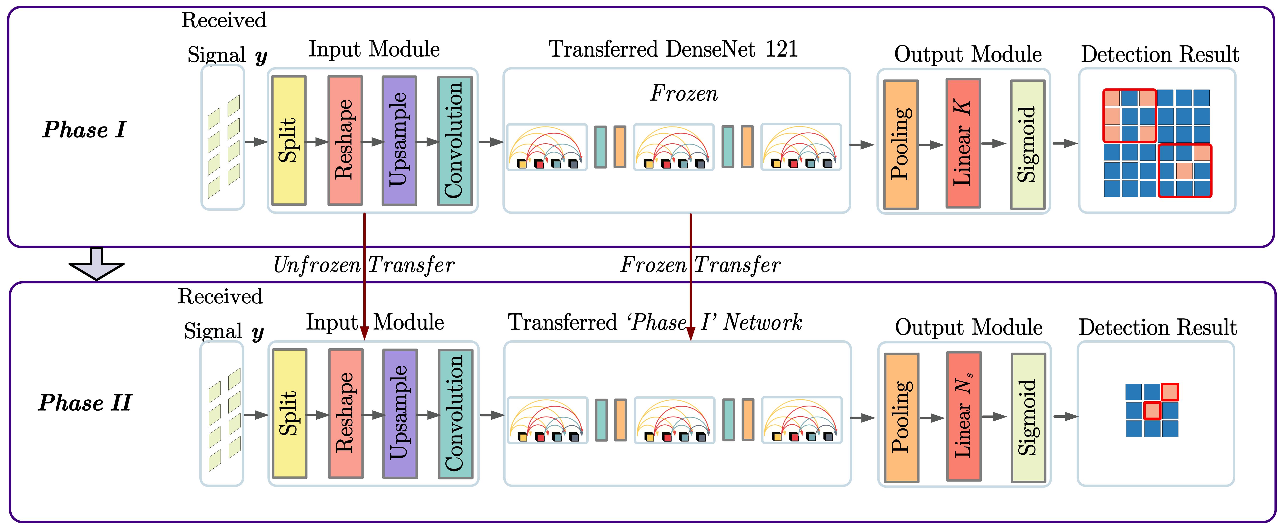
Figure 1: Network structure of TPTL algorithm.

Remark 1.

Given the nature of the received signal $\bm{y}$ at the BS, $\bm{y}$ can be regarded as an image, drawing parallels between problem (P1) and tasks in computer science (CS) [45]. Since the status of the individual elements, ${\mathcal{B}}_{n}$, is either $1$ or $0$, the estimation of the fault status corresponds to a binary classification problem. Furthermore, considering that the RIS comprises multiple elements, (P1) can be regarded as a multi-label classification problem.

Remark 2.

Contemporary research on multi-label classification has only advanced to handle datasets with up to $100$ labels [48]. For instance, datasets like “MS-COCO” encompass $122,218$ images spanning $80$ labels [49]. However, the number of the reflecting elements of an RIS can easily surpass $100$ (e.g., $N_{1}\times N_{2}>10\times 10$). In other words, the number of the labels that need to be classified will exceed $100$ and reach thousands, posing a significant challenge for detecting faulty elements using the existing DL algorithms.

To address the challenge in Remark 2, we propose to divide the RIS panel into multiple SAs, each containing a same number of reflecting elements. Then, Problem (P1) is decomposed into two sub-problems. The first sub-problem is to detect the SA containing the faulty elements (referred to as the “faulty SA”), represented by Problem (P1-a). The second sub-problem is to detect the faulty elements within the faulty SA, represented by Problem (P1-b). These two sub-problems will be sequentially introduced in the following.

III-A1 Detection of Faulty SA

To begin with, let us introduce the procedures for dividing and labeling the SAs. The RIS with $N$ elements is divided into $K$ SAs, with each SA containing $N_{s}=\lfloor N/K\rfloor$ reflecting elements . If the $k$-th SA contains one or more faulty reflecting elements, we classify it as a faulty SA. Conversely, if the $k$-th SA does not contain any faulty elements, we determine the $k$-th SA to be operating correctly. Then, by denoting the number of faulty elements of the $k$-th SA as $N_{k}^{(\textrm{faulty})}$, the status of the $k$-th SA can be mathematically defined as

$$\mathcal{C}_{k}=\begin{cases}0,N_{k}^{(\textrm{faulty})}\geq 1,\\ 1,N_{k}^{(\textrm{faulty})}=0,\quad k\in\{1,\cdots,K\}.\\ \end{cases}$$ (13)

By collecting the status of all SAs in vector form, we have $\bm{\mathcal{C}}=[\mathcal{C}_{1},\cdots,\mathcal{C}_{K}]^{T}$. The estimate of $\bm{\mathcal{C}}$ is thus defined as $\hat{\bm{\mathcal{C}}}=\mathcal{X}({\bm{y}})=[\hat{\mathcal{C}}_{1},\cdots,\hat{\mathcal{C}}_{K}]^{T}$, where $\mathcal{X}(\cdot)$ denotes a non-linear function and $\hat{\mathcal{C}}_{k}$ denotes an estimate of ${\mathcal{C}}_{k}$.

Building upon this, the problem of detecting the faulty SAs can be formulated as follows

$$\textrm{(P1-a)}\quad\underset{\hat{\bm{\mathcal{C}}}}{\min}\quad\mathcal{L}_{\mathcal{C}}\left(\mathcal{X}\left(\bm{y}\right),\bm{{\bm{\mathcal{C}}}}\right),$$ (14)

where $\mathcal{L}_{\mathcal{C}}$ denotes the specific loss function for estimating the status of all SAs.

III-A2 Detection of Faulty Elements of SA

After identifying the faulty SAs, the next step is to detect the faulty elements within a given faulty SA. Similar to (7), the statuses of the faulty elements within the $k$-th faulty SA can be organized in a vector, denoted as $\bm{\mathcal{B}}^{(k)}_{sub}=[\mathcal{B}_{1},\cdots,\mathcal{B}_{N_{s}}]^{T}$. Thus, the estimate of $\bm{\mathcal{B}}^{(k)}_{sub}$ can be written as $\hat{\bm{\mathcal{B}}}^{(k)}_{sub}=[\hat{\mathcal{B}}^{(k)}_{1},\cdots,\hat{\mathcal{B}}^{(k)}_{N_{s}}]^{T}$, where $\hat{\mathcal{B}}^{(k)}_{n_{s}}$, $n_{s}\in\{1,\cdots,N_{s}\}$, represents the estimated status of the $n_{s}$-th element within the $k$-th faulty SA. Besides, we have $\mathcal{H}(\cdot)$ to denote the complex non-linear function between the received signal ${\bm{y}}$ and the estimated statuses of faulty elements within the $k$-th faulty SA.

Consequently, detecting the faulty elements within the $k$-th faulty SA can be formulated as follows

$$\textrm{(P1-b)}\quad\underset{\hat{\bm{\mathcal{B}}}^{(k)}_{sub}}{\min}\quad\mathcal{L}_{\mathcal{B}_{sub}}\left(\mathcal{H}\left(\bm{y}\right),\bm{\mathcal{B}}^{(k)}_{sub}\right),$$ (15)

where $\mathcal{L}_{\mathcal{B}_{sub}}$ denotes the specific loss function for predicting the statuses of the faulty elements within the $k$-th faulty SA.

Similar to (P1), these two sub-problems can also be regarded as a kind of multi-label classification problem. In the field of CS, the multi-label classification problem can be solved by using a CNN [45]. Notably, the parameters of the CNN have to be trained with a large number of data sets before being used in the online phase [45]. However, training two CNN networks to solve the above problems is inefficient. To address this challenge and to save time and computation resources, we propose to leverage transfer learning algorithms [40] to fine-tune pre-trained CNN networks.

III-B Localization Problem Under Faulty Elements

The localization accuracy of existing localization algorithms designed under assumption of a perfect RIS is expected to deteriorate in the presence of faulty RIS elements. Therefore, building upon the obtained knowledge on the faulty elements, i.e., $\hat{\bm{\mathcal{B}}}$, it is crucial to develop a localization algorithm rather that can correct the harmful impact of faulty elements. By defining the estimate of the position of the MU as $\bm{\hat{p}}_{u}$, the relationship with the knowledge of faulty elements can be expressed as

$$\bm{\hat{p}}_{u}=\mathcal{Q}({\bm{y}},\bm{\hat{\mathcal{B}}})=[\hat{x}_{u},\hat{y}_{u},\hat{z}_{u}]^{T},$$ (16)

where $\mathcal{Q}(\cdot)$ represents the intricate non-linear mapping between received signal ${\bm{y}}$ and the estimated position of the MU, $\bm{\hat{p}}_{u}$. In the next step, we tackle the localization problem, labeled as (P2). This problem aims to accurately predict the 3D position of the MU by minimizing the loss function, $\mathcal{L}_{\bm{p}}$. Mathematically, it is formulated as

$$\textrm{({P}2)}\quad\underset{\bm{\hat{p}}_{u}}{\min}\ \mathcal{L}_{\bm{p}}\left(\mathcal{Q}({\bm{y}},\bm{\hat{\mathcal{B}}}),\bm{{p}}_{u}\right).$$ (17)

Traditional convex optimization and channel estimation methods, as highlighted in [19], are not capable of accurately estimating $\bm{{p}}_{u}$. Therefore, this paper introduces a fingerprint-based algorithm for this purpose. After the faulty elements have been identified, we reconstruct from the low-dimensional BS signal to complete high-dimensional RIS signal. This reconstructed RIS received signal then acts as a unique fingerprint for estimating $\bm{{p}}_{u}$. For comparison, we also utilize the BS received signal as another fingerprint to estimate $\bm{{p}}_{u}$.

IV Transfer Learning Empowered Faulty Element Detection Algorithm Design

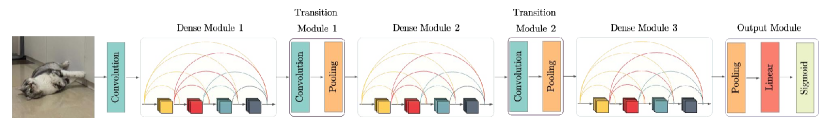
Figure 2: Network structure of DenseNet 121.

In this section, we aim to solve Problem (P1) to estimate the fault statuses of the RIS elements which serves as the foundation for the design of the proposed localization algorithms. To this end, we propose a TPTL algorithm, whose the network structure is depicted in Fig. 1. TPTL employs transfer learning in two distinct phases to sequentially tackle problems (P1-a) and (P1-b). Before introducing the proposed TPTL, we first explain why the transfer learning [40] is adopted in the following subsection.

IV-A Adoption of Transfer Learning

Transfer learning [40] is particularly advantageous for tasks like detecting faulty elements within the RIS. One of the primary reasons behind its suitability is the analogous nature of received signals to images. Received signal ${\bm{y}}$ can be viewed as an image, also with features to be extracted and recognized. This similarity allows us to harness the power of models pre-trained for image recognition tasks and adapt them for faulty elements detection. Transfer learning can efficiently use data from image domains to facilitate faulty elements detection.

Hence, we propose a TPTL algorithm to sequentially address problems (P1-a) and (P1-b). As shown in Fig. 1, during Phase I, we utilize the classical DenseNet 121 [43] as the base model for transfer learning, adapting the input and output modules for Problem (P1-a). Upon completing Phase I training, we save the trained NN to serve as the base model for transfer learning in Phase II. Furthermore, in Phase II, we make necessary adjustments to both the input and output modules of the well-trained model to better fit Problem (P1-b). To facilitate an intuitive understanding of the employed approach, the details of DenseNet 121 will be introduced in the following subsection.

IV-B The Architecture of DenseNet 121

DenseNet [43], inspired by the foundational principles of ResNet [44], reuses the features from earlier layers. However, different from the skip connections which might bypass a couple of layers, DenseNet establishes connections between every layer and every other layer, ensuring a more robust feature propagation. This approach, while reducing the parameter count, allows DenseNet to potentially surpass the performance of ResNet. The design of DenseNet 121 is illustrated in Fig. 2, and its architecture comprises three main components: Dense Modules, Transition Modules, and an Output Module, which will be introduced as follows.

IV-B1 Dense Module

As depicted in Fig. 2, the Dense Module comprises multiple Dense Blocks. The details of a Dense Block are shown in Fig. 3. Each Dense Block starts with a batch normalization (BN) layer, followed by a layer rectified linear unit (ReLU) activation function layer, and concludes with a $3\times 3$ convolutional (Con) layer. A notable characteristic of the Dense Module is its connectivity: Every block incorporates the feature maps of all preceding blocks within the module. This design ensures efficient feature reuse and a rich flow of information throughout the network [43].

IV-B2 Transition Module

From Fig. 2, we observe that the Transition Module, which acts as a connector between Dense Modules, starts with a $1\times 1$ Con layer, followed by a $2\times 2$ average pooling layer, effectively reducing the spatial dimensions of the feature maps and streamlining them for either the next Dense Module or the concluding output layer.

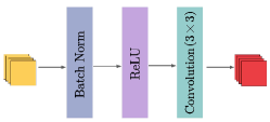
Figure 3: Network structure of a Dense Block.

IV-B3 Output Module

This module employs average pooling to aggregate the feature maps. Subsequently, these integrated features are channeled through a linear layer. A sigmoid activation function then finalizes the process, ensuring that the output values lie between $0$ and $1$.

Having detailed the architecture of DenseNet 121, we will now explain the proposed TPTL algorithm, which is structured in two distinct phases. These phases are elaborated in the following subsections.

IV-C Phase I: Transfer Learning of DenseNet 121

To extract the features from the received signal $\bm{y}$ and tackle sub-problem (P1-a), we employ transfer learning [40] with a pre-trained DenseNet 121 [43]. Though the internal layers of DenseNet 121 are effective at feature extraction due to their extensive pre-training on datasets such as ImageNet [50], adjustments are necessary to cater to the specific nuances of sub-problem (P1-a) and the nature of signal $\bm{y}$. As shown in Fig. 1, an Input Module is introduced to preprocess the received signal, while the Output Module is configured to classify the different statuses of the SAs on the RIS panel. Additionally, choosing an appropriate loss function for this binary classification problem is crucial. The details will be discussed in the subsequent paragraphs.

IV-C1 Input Module

The received signal at the BS, i.e., $\bm{y}$, is first processed by the Input Module so that it can be fed into the transferred DenseNet 121 for classifying the statuses of the SAs [40]. To this end, we first decompose signal $\bm{y}$ as follows

$$\bm{y}=\mathfrak{R}(\bm{y})+j\mathfrak{I}(\bm{y}),$$ (18)

where $\mathfrak{R}(\bm{y})$ and $\mathfrak{I}(\bm{y})$ are the real and imaginary parts, respectively. In this way, we can ensure that both the real and imaginary information contributes to enhancing signal differentiation and facilitating feature extraction.

Thereafter, we reshape both $\mathfrak{R}(\bm{y})$ and $\mathfrak{I}(\bm{y})$ into matrices, which are denoted as ${\bm{M}}_{Ry}\in\mathbb{R}^{M_{1}\times M_{2}}$ and ${\bm{M}}_{Iy}\in\mathbb{R}^{M_{1}\times M_{2}}$, respectively. The primary motivation for this particular reshaping strategy is to effectively extract meaningful features from the UPA of the BS, which spans both the horizontal and vertical dimensions. Then, we concatenate the reshaped matrices of the real and imaginary parts, resulting in a 3D tensor represented as

$$\bm{T}_{y}=\begin{bmatrix}{\bm{M}}_{Ry}\\ {\bm{M}}_{Iy}\end{bmatrix}\in\mathbb{R}^{2\times M_{1}\times M_{2}}.$$ (19)

However, the values of $M_{1}$ and $M_{2}$ may not be directly compatible with DenseNet 121. Hence, an upsampling technique is applied:

$$\bm{T}_{\text{up}}=\text{Upsample}(\bm{T}_{y})\in\mathbb{R}^{2\times 256\times 256}.$$ (20)

The upsampling technique is employed to adjust the dimensions of the tensor $\bm{T}_{y}$ to the desired dimensions of $2\times 256\times 256$. It typically involves pixel value interpolation to expand the image or tensor size, redistributing pixel values accordingly. To make $\bm{T}_{\text{up}}$ suitable for processing by DenseNet 121 [43], which expects an input tensor of the form $(3,256,256)$, a Con Layer is introduced to transform the bi-channel tensor to a tri-channel one:

$$\bm{T}_{\text{DenseNet}}=\text{ConLayer}(\bm{T}_{\text{up}}).$$ (21)

IV-C2 Transferred DenseNet 121

$\bm{T}_{\text{DenseNet}}$ is input to the well-trained DenseNet 121 without the first Con layer and Output Module. While the internal layers of DenseNet 121 are frozen during the early stages of training to maintain their feature extraction capabilities, they are gradually unfrozen later, enabling minor adjustments to adapt better to the specific task of detecting faulty SAs. This ensures that the network leverages the generic feature extraction capabilities of the pre-trained model while also fine-tuning specific layers to our dataset and problem definition for SA detection.

IV-C3 Output Module

In the typical use case, DenseNet 121 is employed for single-label image classification using a softmax layer to determine category probabilities [51]. However, our task in (P1-a) entails a multi-label binary classification problem concerning the statuses of the SAs. Specifically, we have $K$ SAs, and for each one, the goal is to determine if it is faulty or not. The status of a given SA is independent of the statuses of the other SAs. To accommodate this, we modify the linear layer of the Output Module to produce $K$ outputs, which is aligned with the number of SAs under consideration. Furthermore, we replace the softmax layer with the sigmoid layer [51], which allows for individual probability estimation for each label. Defining the output from the linear layer by $\bm{x}_{\textrm{p1}}$, the probability that the $k$-th SA is faulty (represented as $\hat{\mathcal{C}}_{k}=0$) can be expressed as

$$P(\hat{\mathcal{C}}_{k}=0|\bm{x}_{\textrm{p1}})={F}_{\textrm{sig}}(\bm{w}_{k}^{T}\cdot\bm{x}_{\textrm{p1}}+b_{k}),$$ (22)

where ${F}_{\textrm{sig}}$ denotes the employed sigmoid function, $\bm{w}_{k}$ is the weight vector associated with the $k$-th SA, and $b_{k}$ represents the corresponding bias.

IV-C4 Loss Function

For addressing the complexities of our multi-label classification task, it is imperative to employ a suitable loss function. The multi-label soft margin loss in [52] is employed as the specific loss function for addressing the multi-label classification problem in this paper. The application of the multi-label soft margin loss is motivated by its design, specifically tailored for multi-label scenarios [51]. Unlike conventional loss functions, the multi-label soft margin loss was constructed for problems where input samples might simultaneously belong to multiple labels, providing the means to individually estimate label probabilities. The mathematical formulation of the loss function is given by

$$L_{msml}=-\frac{1}{K}\sum_{k=1}^{K}[\mathcal{C}_{k}\log(\hat{\mathcal{C}}_{k})+(1-\mathcal{C}_{k})\log(1-\hat{\mathcal{C}}_{k})],$$ (23)

where $K$ represents the total number of SAs (or labels) in the RIS. For the $k$-th SA, $\mathcal{C}_{k}$ denotes the true label, while $\hat{\mathcal{C}}_{k}$ represents the predicted label.

IV-C5 Training for Faulty SA Detection

Once the Input Module, Output Module, and loss function adjustments are established for the SA classification, the next step is to fine-tune the pre-trained DenseNet 121 on our specific dataset for detecting faulty SAs. This means that we train the model on a new dataset specifically focused on detecting faulty SAs. The utilization of weights initialized from prior training on comprehensive datasets, such as ImageNet [50], offers a foundation that aids faster convergence and potentially better generalization [40].

The primary objective during the training step is to optimize the network weights by minimizing the loss $L_{\mathcal{C}}$, which is specifically designed for the faulty SA detection problem (P1-a). By training and converging the network, Problem (P1-a) of estimating the faulty SAs of the RIS can be solved. The training process involves iteratively adjusting the network weights based on the gradient of the loss with respect to the weights. Mathematically, the optimization problem for training in Phase I can be expressed as

$$\min_{\bm{\theta}_{\textrm{P1-a}}}L_{\mathcal{C}}(\bm{\theta}_{\textrm{P1-a}}),$$ (24)

where $\bm{\theta}_{\textrm{P1-a}}$ represents the parameters (or weights) of the designed network for the detection of faulty SAs in Phase I.

IV-C6 Output after Training

Upon training convergence, the network outputs undergo the sigmoid activation function as detailed previously. This produces probabilities for each status of the faulty SA. The classification based on a threshold of $0.5$ is given by

$$\hat{\mathcal{C}}_{k}=\begin{cases}0&\text{if }P(\hat{\mathcal{C}}_{k}=0|\bm{x}_{\textrm{p1}})\geq 0.5;\\ 1&\text{otherwise}.\end{cases}$$ (25)

Besides, the threshold can be tailored to meet precision-recall needs or practical requirements .

IV-D Phase II: Transfer Learning of ‘Phase I’ Network

Problem (P1-b) is similar to Problem (P1-a), since they have the same prior knowledge $\bm{y}$ and are both muti-label classification tasks. Hence, transfer learning is employed in this phase to reduce the training time and cost. Specifically, we adopt the well-trained NN from Phase I as the base model for transfer learning in Phase II.

If $\mathcal{F}_{1}$ denotes the feature space shaped in Phase I and $\mathcal{F}_{2}$ represents the desired feature space for Phase II, our intent is to discern a transformation function $\phi:\mathcal{F}_{1}\rightarrow\mathcal{F}_{2}$ that minimizes the divergence between these spaces, which is expressed as

$$\phi^{*}=\arg\min_{\phi}\lVert\mathcal{F}_{1}-\phi(\mathcal{F}_{2})\rVert^{2}.$$ (26)

Leveraging the NN pre-trained in Phase I as the base model, we introduce modifications tailored for Phase II, especially in the Output Module. By doing so, we can ensure that the foundational features and representations learned in Phase I remain intact while the network is trained to better align with the task of Phase II. The network structure of Phase II is shown in Fig. 1. Details of the modifications are presented in the following.

IV-D1 Input Module of Phase II

Although Phase II directly transfers the input module from Phase I, it is essential to unfreeze this module before training. This is due to the distinct tasks associated with each phase. This operation aids the network to adapt more effectively to the new problem.

IV-D2 Output Module

To tackle Problem (P1-b), it is imperative to make adjustments to the linear layer within the Output Module. Specifically, the output dimension of this linear layer needs to be adjusted to $N_{s}$. Hence, the Output Module can yield the probabilities associated with the fault statuses of the $N_{s}$ reflecting elements in the $k$-th SA. Denoting the output of this modified linear layer by $\bm{x}_{\textrm{p2}}$, the probability of the $n_{s}$-th reflecting element in the $k$-th SA being faulty (denoted as $\hat{\mathcal{B}}_{n_{s}}^{(k)}=0$) can be expressed as

$$P(\hat{\mathcal{B}}_{n_{s}}^{(k)}=0|\bm{x}_{\textrm{p2}})={F}_{\textrm{sig}}(\bm{w}_{n_{s}}^{T}\cdot\bm{x}_{\textrm{p2}}+b_{n_{s}}),$$ (27)

where $\bm{w}_{n_{s}}$ denotes the weight vector associated with the ${n_{s}}$-th reflecting element and $b_{n_{s}}$ represents the corresponding bias.

IV-D3 Training for Phase II

Once the adjustments have been made, the next step is fine-tuning the pre-trained NN of Phase I on another specific dataset for detecting faulty reflecting elements within each faulty SA. This means that we have to train the model on a new dataset for detecting faulty reflecting elements.

The primary objective during the training step is to optimize the network weights by minimizing the loss $\mathcal{L}_{\mathcal{B}_{sub}}$, which is specifically designed for the faulty reflecting elements detection Problem (P1-b). By training and converging the network using this optimization, Problem (P1-b) of estimating the faulty reflecting elements can be solved. Mathematically, the optimization problem for training in Phase II can be formulated as

$$\min_{\bm{\theta}_{\textrm{P1-b}}}\mathcal{L}_{\mathcal{B}_{sub}}(\bm{\theta}_{\textrm{P1-b}}),$$ (28)

where $\bm{\theta}_{\textrm{P1-b}}$ denotes the parameters (or weights) of the network for this specific sub-problem. Using the gradient of the loss with respect to these weights, the training process iteratively adjusts the network weights until convergence.

Crucially, for Phase II, the internal layers of the NN transferred from Phase I are initially frozen during the early stages of training to retain their feature extraction prowess. However, as training progresses, these layers are gradually unfrozen, allowing for better adaptation to the specific task of detecting faulty reflecting elements. This allows the network to use the pre-trained model’s general features and fine-tune specific layers for detecting faulty reflecting elements.

IV-D4 Output after Training

Upon training convergence, the network outputs are fed into a the sigmoid activation function. This produces probabilities for each status of the reflecting elements within the SA. A threshold, typically set at $0.5$, determines the binary classification:

$$\hat{\mathcal{B}}_{n_{s}}^{(k)}=\begin{cases}0&\text{if }P(\hat{\mathcal{B}}_{n_{s}}^{(k)}=0|\bm{x}_{\textrm{p2}})\geq 0.5,\\ 1&\text{otherwise}.\end{cases}$$ (29)

The threshold can be adjusted based on specific precision-recall requirements or based on the practical requirements.

IV-E Trained TPTL Algorithm Usage Guide

After training of the TPTL algorithm, we integrate the well-trained models into a ‘sealed black box’. Below are the instructions for using the TPTL algorithm to detect the position of faulty elements on the RIS.

IV-E1 Phase I (Diagnosis of Faulty SAs)

The MU acts as a diagnostic device, transmitting a pilot signal towards the BS via the RIS. The received signal at the BS is then input to the well-trained model of Phase I to output the statuses of the SAs within the RIS panel.

IV-E2 Phase II (Diagnosis of Faulty Elements within Detected SA)

After identifying a faulty SA, all other SAs are turned off, and the MU sends another pilot signal to the BS. The received signal at the BS is then input to the well-trained model of Phase II to estimate the faulty statuses of the elements within this faulty SA. This method effectively utilizes the comprehensive information provided by the BS received signal to distinguish between varying faulty scenarios across SAs, thereby demonstrating the versatility and robustness of our proposed diagnostic approach in Phase II.

By sequentially addressing Problem (P1-a) and Problem (P1-b) with the TPTL algorithm, the overall Problem (P1) is resolved.

V Transfer-Enhanced Dual-Stage Algorithm: RIS Signal Reconstruction and Localization

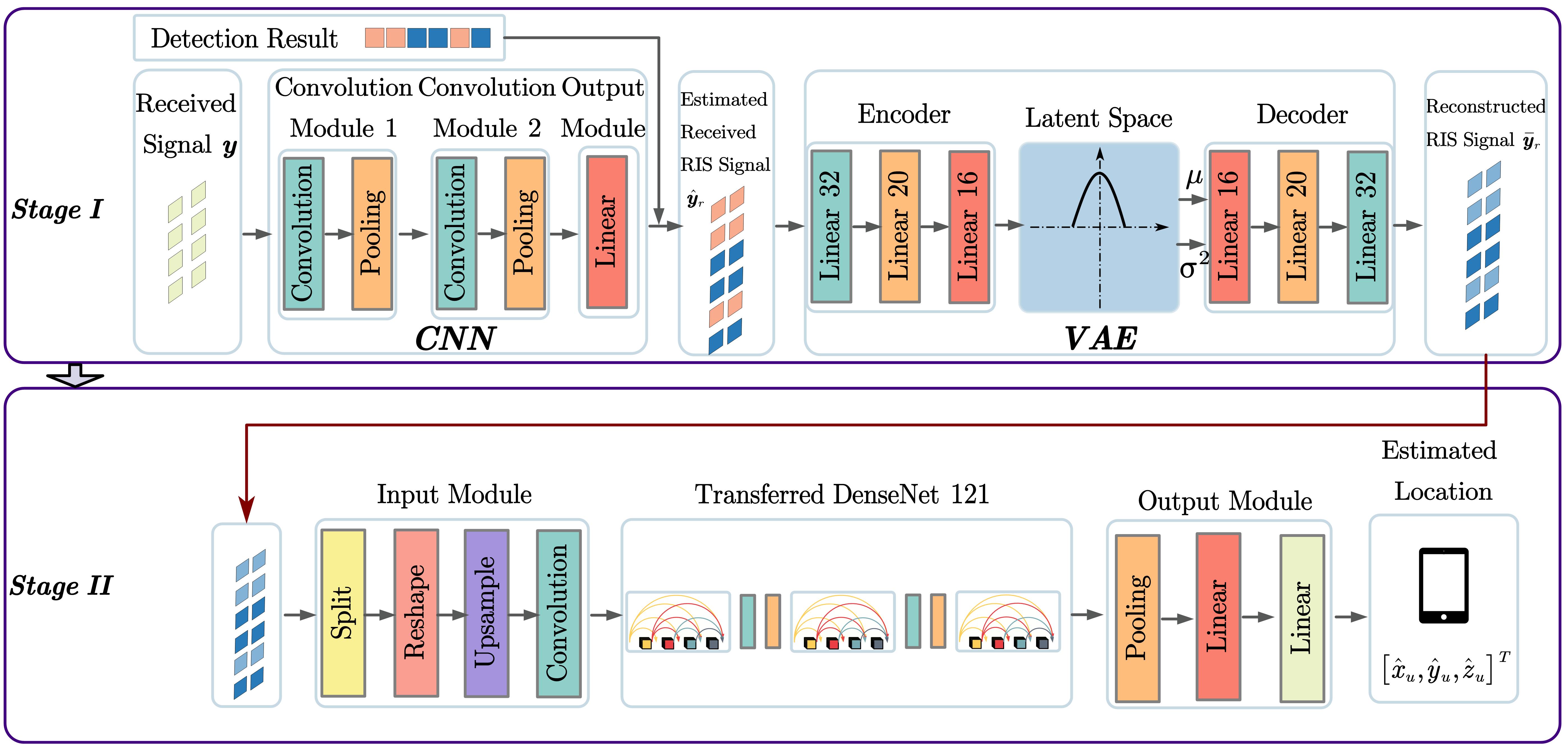
Figure 4: Network structure of TEDS algorithm.

After having identified the faulty elements, our primary aim is to mitigate their detrimental effects and fully realize the potential of high-dimensional RIS information for localization. Addressing this, we introduce the proposed TEDS algorithm, whose network structure is depicted in Fig. 4. Deriving a closed-form solution for the 3D coordinates of the MU using traditional optimization methods is generally impossible [19]. Fingerprint-based methods emerge as an enticing solution, utilizing the received signal as a unique fingerprint to determine the MU’s location [53]. The proposed TEDS algorithm employs the fingerprint-based method, exploiting the high-dimensional RIS information which includes rich information beneficial for localization. As shown in Fig. 4, in Stage I, the focus is on reconstructing the complete high-dimensional RIS received signal based on the lower-dimensonal BS received signal, while Stage II employs the reconstructed RIS information to accurately localize the MU.

V-A Stage I: RIS Signal Reconstruction

To enhance localization performance, it is imperative to restore the information lost due to the identified faulty elements. To this end, the primary objective of Stage I is the reconstruction of the complete high-dimensional signal received at the RIS. As shown in the top half of Fig. 4, Stage I is based on an integrated approach using a CNN followed by a VAE [54]. Specifically, as shown in Fig. 4, given ${\bm{y}}$, the CNN is employed to recover the signal from the non-faulty elements. Then, given the identified faulty elements and the signal from the non-faulty elements, we restore the signal lost by the faulty elements with the VAE. We will first explain the rationale behind choosing the integrated CNN-VAE network, and subsequently outline the corresponding operational details. Finally, the integrated CNN-VAE network is described.

V-A1 Rationale for adapting CNN-VAE Network

Rationale for using CNN

CNNs are good at capturing complex function mappings and predicting continuous outputs, especially with a regression component [45]. They effectively extract spatial features from signals using their Con layers [44].

Rationale for using VAE

VAE renowned for their adept data reconstruction from deficient inputs, emerge as a viable solution for image restoration [54]. Applying to the reconstruction of the high-dimensional RIS received signal, VAE can capitalize on spatial correlations and the information of non-faulty elements. This enable VAE to learn the latent distribution of the input incomplete RIS signals, subsequently generating the complete RIS received signal in alignment with this distribution [54].

Rationale for Integrating CNN and VAE

The integration of the CNN and VAE models provides significant benefits. Training them jointly allows shared feature extraction, improving model performance. This approach saves computational resources by avoiding multiple passes in separate networks and uses a single loss function for consistent training, leading to better signal reconstruction.

V-A2 Recovering Signal Recieved from Non-Faulty Elements

To reproduce the incomplete received signal at the RIS with faulty elements, as illustrated in Fig. 4, a combination of a CNN and a regression module is employed, where the CNN is specifically utilized to estimate the signal, denoted as ${\bm{y}}_{r}$. However, due to the architecture of the CNN, its output cannot contain zero values. This leads to a potential misalignment between the CNN’s output and the expected incomplete received signal. To overcome this challenge, we employ status vector $\bm{\mathcal{B}}$, where each element of the vector is either $0$ or $1$. By multiplying the CNN’s output with this status vector, the incomplete received signal at the RIS is successfully reproduced.

CNN Architecture

As depicted in Fig. 4, the proposed CNN has two Convolution Modules followed by an Output Module. Each Convolution Module encompasses a Con layer, a ReLU activation function, and a max-pooling operation. The final Output Module consists of a linear layer with dimension $N_{1}\times N_{2}$.

CNN Training

During training, the primary goal is to condition the CNN, using received signal ${\bm{y}}$ from the BS, to reproduce the received signal at the RIS, denoted as ${\bm{y}}_{r}$. Besides, let us define the output of the employed CNN as $\hat{\bm{y}}_{r}$, which is given by

$$\hat{\bm{y}}_{r}=F_{\text{CNN}}({\bm{y}};{\bm{\theta}}_{cnn})\odot\bm{\mathcal{B}},$$ (30)

where ${\bm{\theta}}_{cnn}$ denotes the set of the parameters (or weights) of the CNN, and $F_{\text{CNN}}$ represents a function mapping ${\bm{y}}$ to $\hat{\bm{y}}_{r}$. The objective of this training is to minimize the error caused by the reproduced signal as follows

$$\min_{{\bm{\theta}}_{cnn}}\ \lVert{\bm{y}}_{r}-\hat{\bm{y}}_{r}\rVert^{2}_{2}.$$ (31)

Upon optimizing this objective, the CNN is conditioned to best recover the incomplete received signals at the RIS panel.

V-A3 Restoring Lost Information from Faulty Elements

After recovering the incomplete RIS received signals through the CNN, $\hat{\bm{y}}_{r}$ undergoes further reconstruction using a VAE as shown in Fig. 4.

VAE Network Architecture

According to Fig. 4, the VAE begins with an encoder that learns the distribution of the input $\hat{\bm{y}}_{r}$ through a series of linear layers. This process results in the establishment of a latent space, which represents the essential features of the data by determining the latent mean $\mu$ and latent variance $\sigma^{2}$. From this latent space, the encoder samples a set of latent variables. The decoder, which consists of another sequence of linear layers, uses these sampled latent variables to reconstruct the output, denoted as $\bar{\bm{y}}_{r}$ , which is an approximation of the input $\hat{\mathbf{y}}_{r}$ intended to be as close to the original input as possible. To be specific, the decoder randomly generates new instances within the latent space that are used to reconstruct the input data.

Training of VAE

With the VAE structure in place, the reconstructed signal $\bar{\bm{y}}_{r}$ can be obtained by feeding $\hat{\bm{y}}_{r}$ through the encoder to get the latent variables, and subsequently passing these variables through the decoder. The specific operations are shown in Fig. 4. Mathematically, the reconstruction process can be represented as follows

$$\bar{\bm{y}}_{r}=F_{\text{VAE}}(\hat{\bm{y}}_{r};{\bm{\theta}}_{vae}),$$ (32)

where ${\bm{\theta}}_{vae}$ denotes the set of parameters (or weights) of the VAE, and $F_{\text{VAE}}$ represents a function mapping $\hat{\bm{y}}_{r}$ to $\bar{\bm{y}}_{r}$. Hence, the optimization problem for this training is formulated as

$$\min_{{\bm{\theta}}_{vae}}\ \lVert\hat{\bm{y}}_{r}-\bar{\bm{y}}_{r}\rVert^{2}_{2}+\text{KL}(L_{v}),$$ (33)

where KL and $L_{v}$ denote the Kullback-Leibler divergence and the latent variables [54]. The inclusion of the KL-term acts as a regularization mechanism, ensuring that the latent variables adhere to a certain distribution. Through this VAE-based reconstruction process, we aim to achieve a more precise and noise-resistant reconstruction of the RIS received signal.

V-A4 Integrated CNN-VAE Network

The proposed integrated network combines the capabilities of CNN and VAE. The CNN is responsible for recovering the incomplete RIS received signal. Following this, the VAE reconstructs the complete RIS received signal.

Training

During training, the model is conditioned using the low-dimensional BS signal, ${\bm{y}}$, to reconstruct complete high-dimensional RIS signal, $\bar{\bm{y}}_{r}$. Simultaneously, the network incorporates the statuses of the faulty elements, $\bm{\hat{\mathcal{B}}}$, to guide the learning process. The objective during training is defined as

$$\min_{{\bm{\theta}}_{cnn},{\bm{\theta}}_{vae}}\Bigg{[}\lVert{\bm{y}}_{r}-\hat{\bm{y}}_{r}\rVert^{2}_{2}+\lVert\hat{\bm{y}}_{r}-\bar{\bm{y}}_{r}\rVert^{2}_{2}+\text{KL}(L_{v})\Bigg{]}.$$ (34)

Output

Upon convergence of training, the network’s parameters ${\bm{\theta}}_{cnn},{\bm{\theta}}_{vae}$ are optimized to reconstruct the RIS received signal. The model can then process any low-dimensional input ${\bm{y}}$ to generate a higher-dimensional output $\bar{\bm{y}}_{r}$.

V-B Stage II: Enhanced Localization using Reconstructed Signal $\bar{\bm{y}}_{r}$

This stage builds upon the reconstructed RIS information, $\bar{\bm{y}}_{r}$, obtained in Stage I. As shown in the lower half of Fig. 4, the primary goal of this phase is to achieve enhanced localization using the reconstructed RIS information as well as the statuses of the elements. Similar to how we tackled the faulty element detection problem in the previous section, we propose to utilize the pre-trained DenseNet 121 for transfer learning to handle the localization problem described in (17). By doing so, we can harness the knowledge of the model acquired from previous tasks [45]. This approach, grounded in the success of transfer learning for image classification [40], is satisfied due to its smaller training times and often achieves better results comparing to the traditional training-from-scratch methods [45]. Hence, we employ a transfer learning approach to localize the MU at Stage II. As depicted in Fig. 4, we input the reconstructed signal $\bar{\bm{y}}_{r}$ as a type of fingerprint to the transferred DenseNet 121 to output the 3D location of the MU.

Before the training process, some modifications of the transferred DenseNet 121 are added to specifically address Problem (P2). The details are given as follows.

V-B1 Input Module

To extract features from $\bar{\bm{y}}_{r}$, we divide it into its real and imaginary parts, represented as $\mathfrak{R}(\bar{\bm{y}}_{r})$ and $\mathfrak{I}(\bar{\bm{y}}_{r})$. These parts are then merged and reshaped based on the UPA antenna setup at the RIS. Since $N_{1}$ and $N_{2}$ may not fit the NN architecture’s input size, we use interpolation techniques to make the signal dimensions compatible with DenseNet. Lastly, a Con layer adjusts the tensor size to meet the DenseNet 121 input requirements.

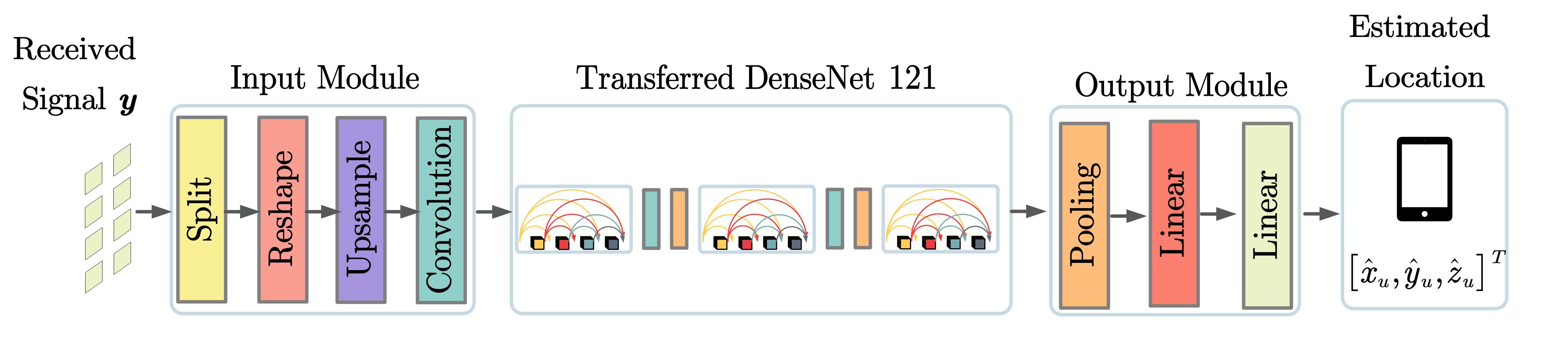
Figure 5: Network structure of TEDF algorithm.

V-B2 Transferred DenseNet 121

After preprocessing the received signal $\bar{\bm{y}}_{r}$, the Input Module outputs the preprocessed tensor to the transferred DenseNet 121. Notably, the internal layers of the transferred DenseNet 121 are initially frozen during the early training stage and gradually unfrozen as training progresses.

V-B3 Output Module

Conventionally, DenseNet 121 employs a softmax layer after the linear layer at the Output Module to yield category probabilities. To cater to the considered regression problem, we replace the softmax layer with a linear layer. This layer comprises three neurons, corresponding to the MU’s coordinates.

V-B4 Selection of the Loss Function

Predicting 3D coordinates is more effectively tackled using regression than classification, given that these coordinates exist in a continuous space rather than discrete categories [25]. Trying to classify each coordinate as a unique category would drastically increase the number of classes, increasing complexity and computational demands [53]. For regression tasks, the mean squared error (MSE) loss is often favored [40]. It measures the discrepancy between predicted and actual values and has continuous derivatives that facilitate optimization. Furthermore, larger errors are penalized more by MSE, which makes the model highly sensitive to significant deviations. Given the importance of precision in 3D coordinate prediction, regression with MSE emerges as a sound and efficient option.

V-B5 Transfer Learning for Localization

Leveraging the foundational weights and configurations from pre-trained models, the focus shifts to training the DenseNet 121 for the task of localization. At this stage, the primary goal is to solve Problem (P2) which is mathematically represented as

$$\min_{\bm{\theta}_{\textrm{loc}}}\mathcal{L}_{\bm{p}}\left(\bm{\theta}_{\textrm{loc}}\right),$$ (35)

where $\bm{\theta}_{\textrm{loc}}$ stands for the parameters (or weights) specific to the localization problem in the transferred DenseNet 121.

V-B6 Localization with well-trained DenseNet

Upon convergence of the training phase, the DenseNet 121 model stands ready to provide estimates for the 3D position of the MU. As we can see from Fig. 4, for every reconstructed RIS singal $\bar{\bm{y}}_{r}$, the network outputs a three-dimensional vector, $[\hat{x}_{u},\hat{y}_{u},\hat{z}_{u}]^{T}$, which is an estimate of the MU’s coordinates. Therefore, Problem (P2) has been effectively solved by the proposed TEDS algorithm.

VI Transfer-Enhanced Direct Fingerprint Algorithm

To be able to show more light on the gain achieved by using RIS information and the impact of faulty RIS elements on localization, in this section, we propose a benchmark algorithm, named TEDF algorithm, which only exploits the BS signal. As depicted in Fig. 5, we directly input the BS received signal ${\bm{y}}$ as a type of fingerprint to the transferred DenseNet 121 to predict the 3D location of the MU. In contrast to TEDS algorithm, this localization algorithm, without relying on RIS information, may suffer from some performance loss. Therefore, the comparison between these two kinds of algorithm can further highlight the necessity of faulty element detection and the benefits of exploiting the high-dimensional RIS signal for localization. The details of this algorithm are provided in the following.

VI-A Transfer Learning for Localization

The TEDF algorithm is also based on the DenseNet 121 model, leveraging its powerful transfer learning capabilities. However, in contrast to the method discussed in the previous section, the input data to this model is the received signal ${\bm{y}}$ at the BS. The fundamental rationale remains unchanged; the DenseNet is capable of deriving intricate spatial relationships from the signal, providing insights into the MU’s position.

VI-B Training Using BS Received Signal

During the training phase, the model learns to map the received signal ${\bm{y}}$ to the actual MU position without knowledge of the faulty elements. In a training process, the model is optimized to reduce discrepancies between the predicted position and the actual MU position, using the same loss functions and methodologies as discussed earlier.

VI-C Localization with Well-trained TEDF Algorithm

After convergence of the training phase, the proposed TEDF algorithm is capable of estimating the 3D position of the MU. For every received BS singal ${\bm{y}}$, the network outputs a three-dimensional vector, $[\hat{x}_{u},\hat{y}_{u},\hat{z}_{u}]^{T}$, which corresponds to the MU coordinates.

VII Simulation Results

In this simulation, we consider a setup in a three-dimensional space, involving a MU, an RIS, and a BS. The carrier frequency is $f=90$ GHz. The RIS is composed of $N_{1}\times N_{2}=81$ elements, with adjacent elements spaced at $d_{r}=\lambda/2=1.67\times 10^{-3}$ m. The center of the RIS is located at $\bm{p}_{r}=(15,0,2)$ m. The BS comprises $M_{1}\times M_{2}=16$ antennas, with an antenna spacing of $d_{b}=\lambda/2=1.67\times 10^{-3}$ m. The center of the BS is positioned at $\bm{p}_{b}=(0,10,1.5)$ m. The MU-RIS link includes $P=10$ propagation paths, and the RIS-BS link comprises $J=10$ propagation paths. The transmit power of the MU is $10$ dBm. The phase shifts of the elements at the RIS are set to a unity matrix.

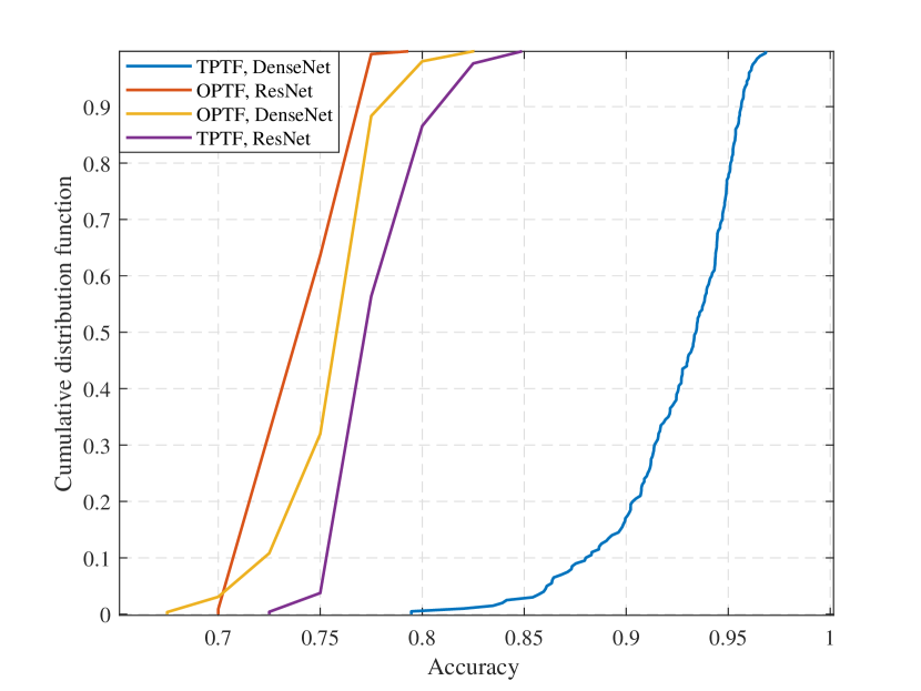
Figure 6: The CDF of detection accuracy with different kinds of algorithm.

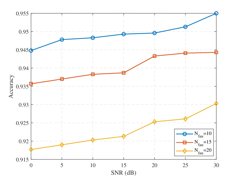
Figure 7: Detection accuracy versus SNR (dB) across different $N_{\textrm{fau}}$.

During the training stage of the proposed TPTL algorithm for detecting the faulty elements of the RIS, we assume the MU is located at $\bm{p}_{u}=(30,6,0.5)$ m, and the number of faulty elements within the RIS is assumed to be no more than $15$, i.e., $N_{\textrm{faul}}\leq 15$. Furthermore, we assume that there are $K=9$ SAs, each containing $N_{s}=9$ reflecting elements. The dataset consists of $20,000$ randomly generated fault scenarios, split into training and testing sets at a ratio of $0.8:0.2$. During the training stage of the proposed TEDF and TEDS algorithms for estimating the location of the MU, we assume that the MU is uniformly distributed within three grids measuring $10$ m in length, $10$ m in width, and heights of $0.5$ m, $1.5$ m, and $2$ m, respectively. The dataset consists of $60,000$ samples, each sample has the MU’s coordinates, the condition of faulty elements on the RIS panel, and the corresponding signals received by both the BS and RIS. The dataset is split into training and testing sets at a ratio of $0.8:0.2$.

Fig. 7 presents the cumulative distribution function (CDF) of faulty element detection accuracy for different algorithms. The blue curve, labeled ‘TPTF DenseNet’, signifies the TPTF algorithm transferring the DenseNet 121 architecture. Conversely, the purple curve, labeled ‘TPTF ResNet’, represents the TPTF algorithm using ResNet 18. Furthermore, the yellow and red curves, labeled ‘OPTF DenseNet’ and ‘OPTF ResNet’ respectively, represent the benchmarks of the one phase transfer learning (OPTF) algorithm transferring DenseNet 121 and ResNet 18. As depicted in Fig. 7, the proposed TPTF, by sequentially detecting the faulty SAs and internal faulty elements, optimally harnesses DenseNet 121 or ResNet 18 for targeted faulty element detection, thus amplifying accuracy. Contrarily, the OPTF algorithm does not first detect the subarrays and then the elements within the subarrays, resulting in the number of elements (or labels) to be classified surpassing the performance capacity of DenseNet (or ResNet). Consequently, the performance of the OPTF algorithm is inferior. Significantly, the proposed ‘TPTF DenseNet’ achieves commendable detection outcomes, with a $80\%$ probability of attaining a $91\%$ detection accuracy, surpassing ‘TPTF ResNet’, ‘OPTF DenseNet’, and ‘OPTF ResNet’, which have the accuracies of $76\%$, $74\%$, and $71\%$ at the identical confidence interval. In summary, Fig. 7 emphasizes the superior detection performance of the propose ‘TPTF DenseNet’ algorithm.

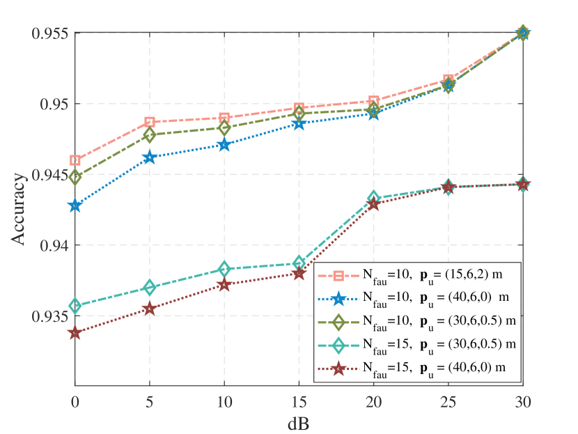
Figure 8: Detection accuracy versus SNR (dB) across different positions and $N_{\textrm{fau}}$.

Fig. 7 presents the detection accuracy of the proposed TPTF algorithm under different signal-to-noise ratios (SNRs), showcasing its performance in test scenarios with a specified number of faulty elements, $N_{\text{fau}}=10,15,20$. These numbers are exclusive to the testing phase. As delineated in Fig. 7, the TPTF algorithm maintains remarkable efficacy, achieving a $92\%$ detection accuracy at an SNR of $10$ dB even faced with $20$ faulty elements. Moreover, in challenging conditions with an SNR as low as $0$ dB, the detection accuracies remain robust at approximately $91.7\%$, $93.6\%$, and $94.5\%$ for $20$, $15$, and $10$ faulty elements, respectively. This underscores the robustness of the proposed TPTF detection algorithm in low SNR scenarios .

In Fig. 8, we delve into the TPTL algorithm’s effectiveness in identifying faulty elements under variable MU locations, particularly focusing on ${\bm{p}}_{u}=(15,6,2)$ m and ${\bm{p}}_{u}=(40,6,0)$ m with up to 10 faulty elements, extending to ${\bm{p}}_{u}=(40,6,0)$ m for scenarios encompassing up to 15 faulty elements. It is observed that there exists a marginal improvement as the distance between the MU and the RIS-BS system narrows, especially in environments characterized by lower SNR values. However, the detection accuracy remains the same when SNR is larger than $20$ dB. This reveals that changes in the MU’s position do have some effect, but it’s not significant. Moreover, as the SNR increases, this impact diminishes.

The essence of these observations lies in their testament to the TPTL algorithm’s versatile performance across diverse spatial arrangements and signal conditions. This demonstrates not just the algorithm’s capability to adjust its performance based on the proximity and configuration of the MU relative to the BS and RIS, but also its robustness and reliability in a variety of operational environments. This versatility is paramount for ensuring the algorithm’s applicability and efficacy in real-world deployments, where environmental and situational variability is the norm.

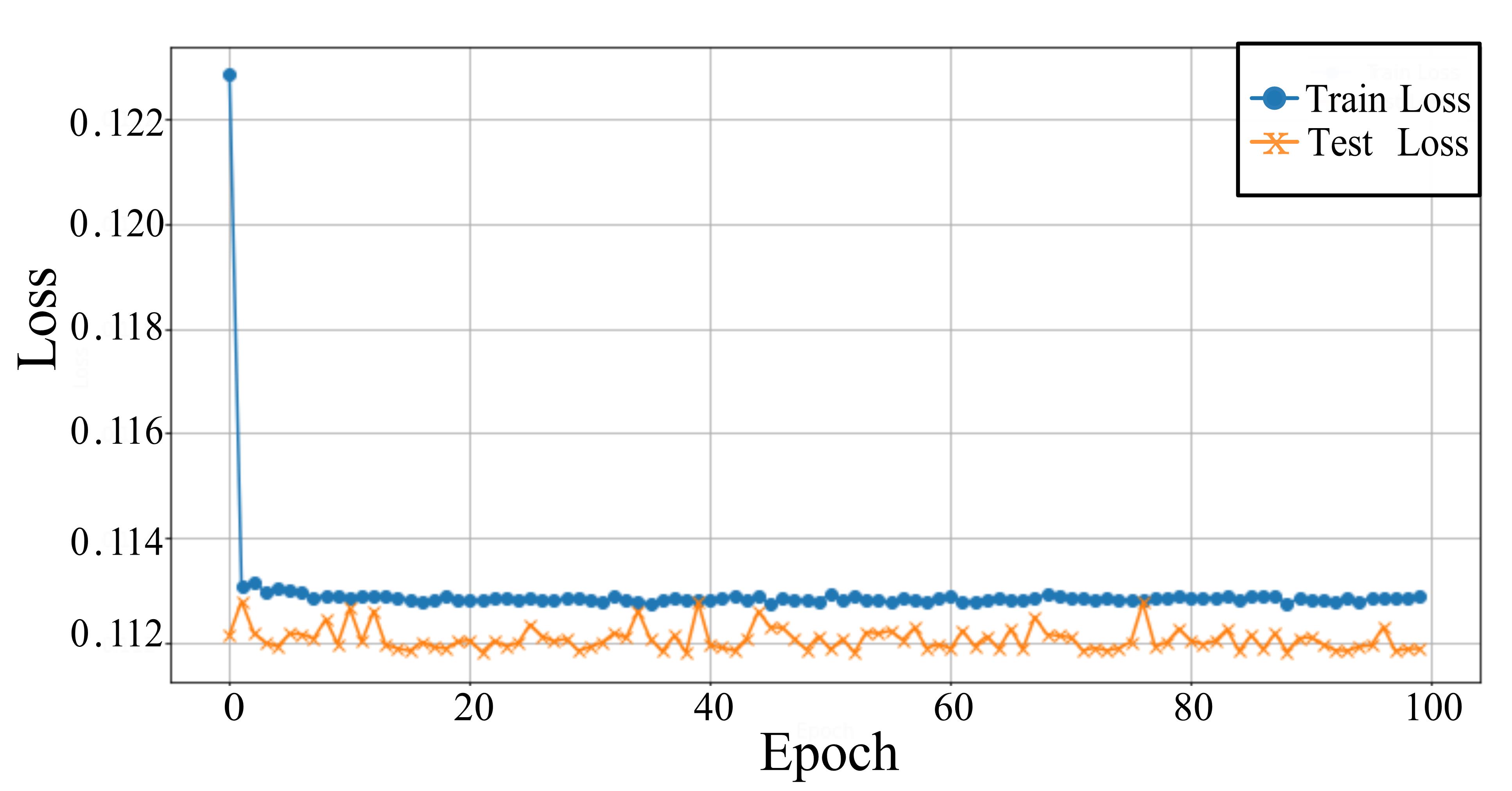
(a) Test loss and train loss of TEDF algorithm.

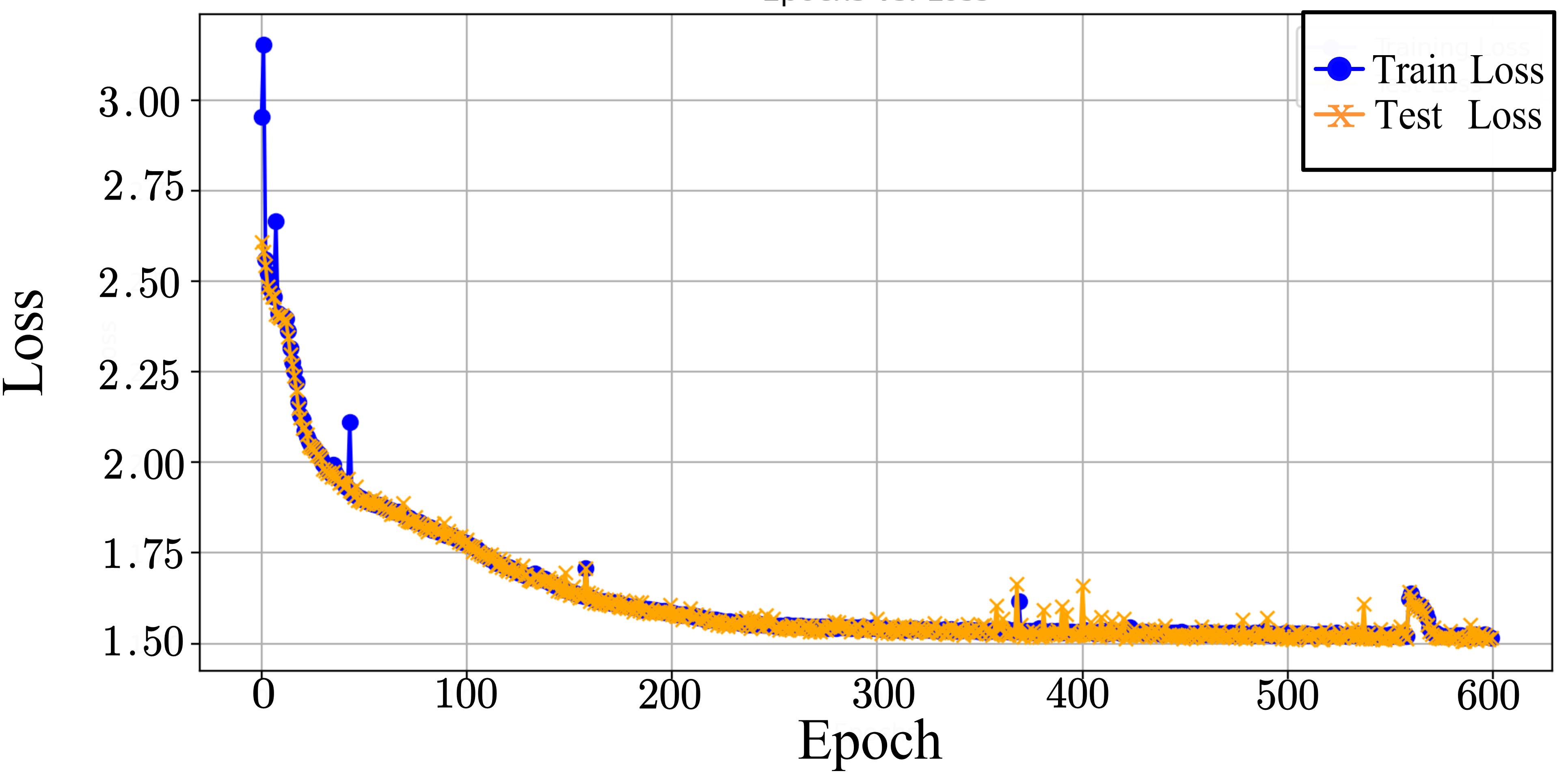
(b) Test loss and train loss of Stage I of TEDS algorithm.

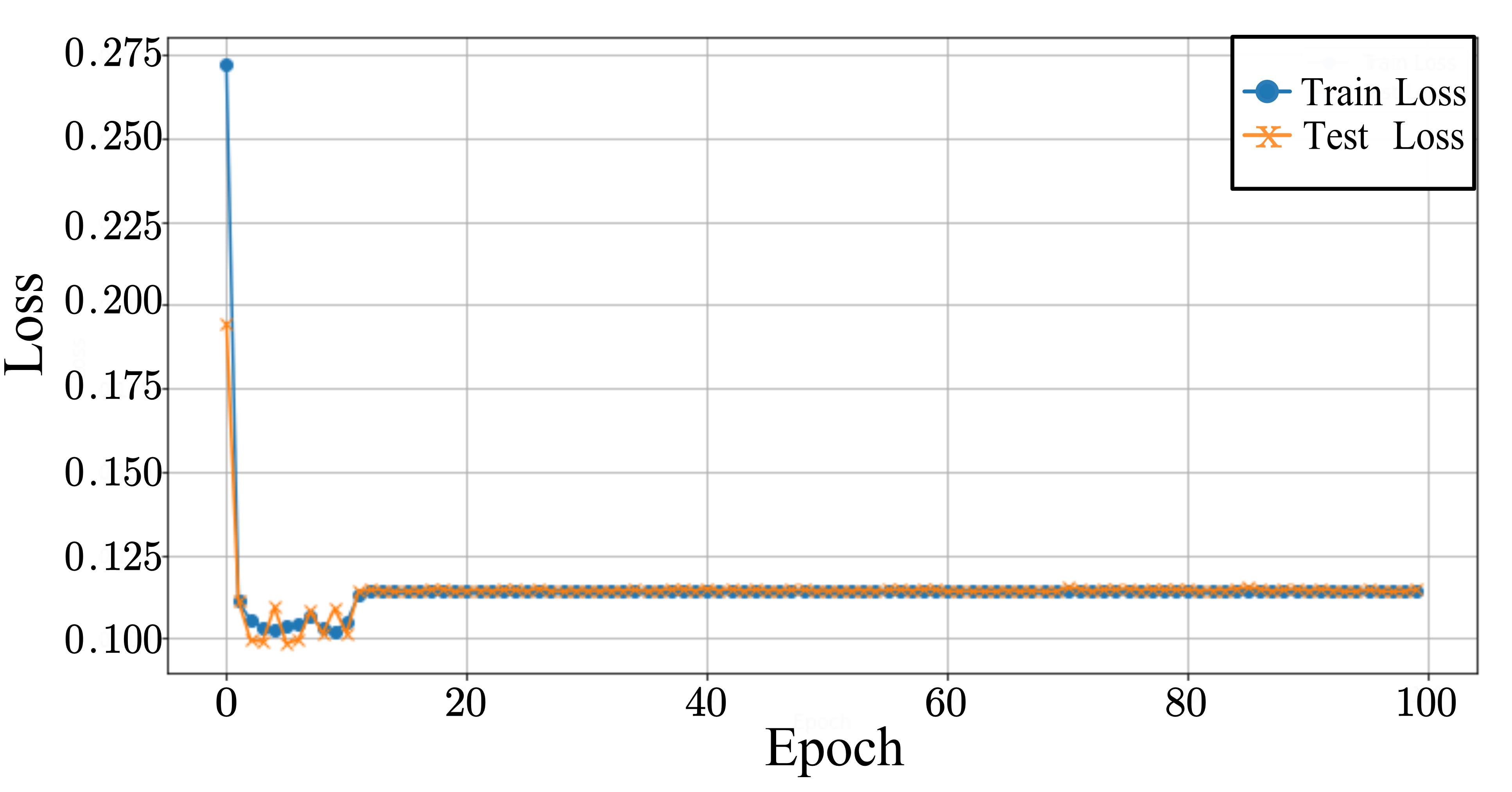
(c) Test loss and train loss of Stage II of TEDS algorithm.

Figure 9: Losses of TEDF algorithm and TEDS algorithm in Stage I and Stage II.

Fig. 9 showcases the train and test loss curves of two algorithms, i.e., TEDF and TEDS, employed for MU coordinate estimation. Specifically, Fig. 9(a) displays the iterative convergence behaviors of train and test losses for the TEDF algorithm. It is evident that by approximately $20$ epochs, both train and test losses for the TEDF algorithm have converged. Although there are minor fluctuations in the test loss afterwards, their magnitude is negligible. Additionally, in Stage I of the TEDS algorithm, we employs the CNN-VAE network, which uses low-dimensional signals, ${\bm{y}}$, to reconstruct complete high-dimensional RIS received signal at the RIS, $\bar{\bm{y}}_{r}$. Fig. 9(b) presents the train and test losses of the proposed CNN-VAE network. During training, there is a rapid decline in both train and test losses initially, followed by a more gradual reduction. This demonstrates the complexity of reconstructing higher-dimensional information from low-dimensional information as well as the challenge of restoring signals expected to be received by faulty elements. The losses appear to stabilize around the $500$-th iteration. Lastly, Fig. 9(c) represents the convergence behavior for train and test loss in Stage II of the TEDS algorithm, where losses converge around the $15$-th epoch with negligible fluctuations. Comparing Fig. 9(c) and Fig. 9(a) which employ transfer learning with Fig. 9(b), the advantages of transfer learning are evident. By leveraging transfer learning, the number of required train epoches is significantly reduced while maintaining accuracy, making it highly suitable for the complex and dynamic environments anticipated in 6G. This offers valuable insights for future RIS-aided localization systems.

Fig. 10 employs normalized mean square error (NMSE) to compare the localization accuracy of the TEDF and TEDS algorithms for $N_{\textrm{fau}}=10$ and $N_{\textrm{fau}}=15$. The curves labeled ‘TEDF, $N_{\textrm{fau}}=10$’ and ‘TEDF, $N_{\textrm{fau}}=15$’ correspond to scenarios using BS information as a fingerprint, while ‘TEDS, $N_{\textrm{fau}}=10$’ and ‘TEDS, $N_{\textrm{fau}}=15$’ represent the utilization of RIS information as a fingerprint for the same $N_{\textrm{fau}}$ values. The figure clearly shows that employing high-dimensional RIS information significantly improves localization performance compared to using lower-dimension BS information, even in the presence of faulty elements. This underscores the advantage of leveraging high-dimensional RIS information. Furthermore, the figure demonstrates that the localization performance remains relatively stable with minimal degradation when the number of faulty elements increases from $10$ to $15$, emphasizing the robustness of the proposed algorithms against faulty element variations.

Fig. 10 also presents the curves representing scenarios where RIS information is used as a fingerprint but without processing through the CNN-VAE network. These scenarios are for RIS with no faulty elements and RIS containing 15 faulty elements, labeled as‘RIS Inf., $N_{\textrm{fau}}=0$’, and ‘RIS Inf., $N_{\textrm{fau}}=15$’, respectively. As a comparison in the picture, the curves ‘TEDS, $N_{\textrm{fau}}=10$’ and ‘TEDS, $N_{\textrm{fau}}=15$’ show a minor gap with the ‘RIS Inf., $N_{\textrm{fau}}=0$’ curve but a significant gap with the ‘RIS Inf., $N_{\textrm{fau}}=15$’curve. This observation suggests the effectiveness of the proposed CNN-VAE network in reconstructing the complete high-dimensional RIS information and demonstrates that we can regain the localization accuracy with the proposed algorithms.

Furthermore, Fig. 10 also presents the scenarios that train the TEDS algorithm with the same loss but without the detection result, which is labeled as ‘w/o Detection, $N_{\text{fau}}=15$’. It is shown that even though without the detection result of the faulty elements, the proposed integrated CNN-VAE network can still reconstruct the essential localization-related information. Additionally, Fig. 10 includes a curve labeled ‘Opt. RIS, $N_{\textrm{fau}}=0$’, which represents scenarios where the information of a RIS without faulty elements is used as a fingerprint, with its phase shifts optimized to maximize the received SNR [46]. As a comparison, there exists marginal gap between ‘Opt. RIS, $N_{\textrm{fau}}=0$’ and ‘RIS Inf., $N_{\textrm{fau}}=0$’, highlighting the robustness of the RIS information based localization algorithm against the unoptimized phase shifts. We conjecture that the reason for this phenomenon lies in that the localization accuracy is dominated by the high-dimensional RIS information, and therefore the phase shift design does not play an important role.

Fig. 11 utilizes NMSE to compare the performance of the TEDF and TEDS algorithms under two distinct SNR conditions, i.e., $\textrm{SNR}=10$ dB and $\textrm{SNR}=30$ dB. The red, purple, green, and orange curves respectively represent ‘TEDF, $\textrm{SNR}=10$ dB’, ‘TEDF, $\textrm{SNR}=30$ dB’, ‘TEDS, $\textrm{SNR}=10$ dB’, and ‘TEDS, $\textrm{SNR}=30$ dB’. As depicted in Fig. 11, the localization performance of the TEDF algorithm exhibits sensitivity to SNR variations, leading to a measurable reduction. In contrast, the TEDS algorithm showcases remarkable robustness against SNR variations, as evidenced by the near overlap of the red and green curves. We conjecture that the reason for this phenomenon lies in that the employed CNN-VAE network can effectively against the variations of SNR. Such observations underscore the superiority of the proposed TEDS algorithm, suggesting that the localization algorithm remains highly effective even in diverse and intricate communication scenarios. This further supports the notion that localization performance can indeed benefit from the high-dimensional RIS information even with the faulty elements.

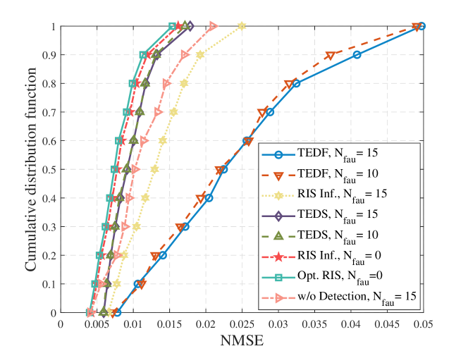
Figure 10: Comparison of TEDF and TEDS algorithms when $N_{\textrm{fau}}=10,15$.

Figure 11: Comparison of TEDF and TEDS algorithms when $\textrm{SNR}=10,30$ dB.

Fig. 12 compares the NMSE of the proposed TEDS algorithm and TEDF algorithm with the near field and far field effects. As shown in Fig. 12, it can be observed that when employing the TEDF algorithm, the localization performance under near-field conditions significantly surpasses that in the far-field. However, with the application of the TEDS algorithm, while localization accuracy in the near-field still outperforms the far-field, the advantage is not as pronounced. We infer that this phenomenon is attributable to the richer localization information available in the near-field. Nonetheless, the dominant role of the high-dimensional RIS information reconstructed by the TEDS algorithm mitigates the disparity in gains between the near and far fields. Moreover, Fig. 12 also corroborates the effectiveness of the proposed algorithm in both near-field and far-field conditions, underscoring its robustness and adaptability across different propagation environments.

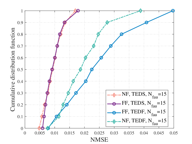
Figure 12: NMSE Comparison between the far field and near field effect when employing the TEDS algorithm and TEDF algorithm.

Fig. 13 compares the NMSE of the proposed TEDS algorithm with the integrated CNN-VAE network and with the CNN-Interpolation method. As shown in Fig. 13, the CNN-Interpolation method shows some improvement over the TEDF algorithm. However, there is still a significant gap when compared to the TEDS algorithm that utilizes the CNN-VAE network. This comparison validates the superiority of our proposed TEDS algorithm, especially in addressing the capability of restoring the lost RIS information .

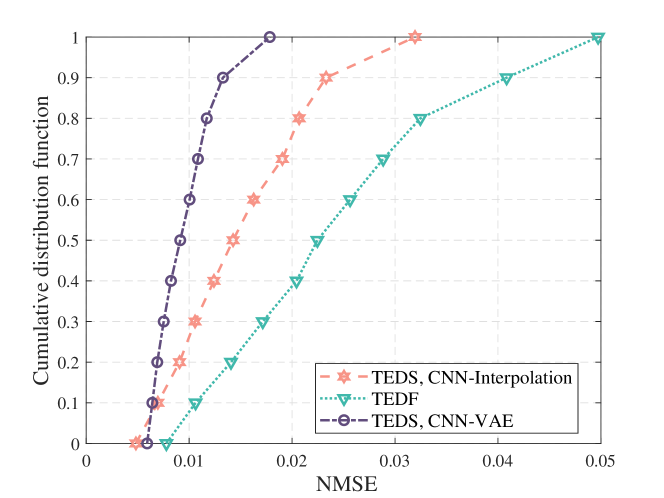
Figure 13: NMSE Comparison between the Integrated CNN-VAE method and the CNN-Interpolation method.

VIII Conclusion

This paper has investigated the localization algorithm design based on the high-dimensional RIS information in the presence of faulty RIS elements. We have designed a TPTL algorithm for faulty element detection. We have proposed a TEDS algorithm to clear their harmful impact, unleashing the gain of RIS on localization. At Stage I, we have reconstructed the complete high-dimensional RIS received signal from the low-dimensional BS received signal. At Stage II, this reconstructed RIS information has been input to the transferred DenseNet to estimate the location of the MU. We have also proposed a low-complexity TEDF algorithm which only utilizes the low-dimensional BS information. Simulation results have demonstrated that we can effectively benefit from the high-dimensional RIS information even with faulty elements.

References

- [1] C.-X. Wang et al., “On the Road to 6G: Visions, Requirements, Key Technologies, and Testbeds,” IEEE Comm. Surv. Tutor., vol. 25, no. 2, pp. 905–974, 2023.
- [2] H. Chen et al., “RISs and Sidelink Communications in Smart Cities: The Key to Seamless Localization and Sensing,” IEEE Commun. Mag., vol. 61, no. 8, pp. 140–146, 2023.
- [3] C.-X. Wang et al., “Pervasive Wireless Channel Modeling Theory and Applications to 6G GBSMs for All Frequency Bands and All Scenarios,” IEEE Trans. Veh. Technol., vol. 71, no. 9, pp. 9159–9173, 2022.
- [4] H. Chen et al., “A Tutorial on Terahertz-Band Localization for 6G Communication Systems,” IEEE Commun. Surv. Tutor., vol. 24, no. 3, pp. 1780–1815, 2022.
- [5] K. Meng et al., “Throughput Maximization for UAV-Enabled Integrated Periodic Sensing and Communication,” IEEE Trans. Wireless Commun., vol. 22, no. 1, pp. 671–687, 2023.
- [6] H. Wymeersch et al., “Radio Localization and Sensing Part II: State-of-the-Art and Challenges,” IEEE Commun. Lett., vol. 26, no. 12, pp. 2821–2825, 2022.
- [7] J. He et al., “Beyond 5G RIS mmWave Systems: Where Communication and Localization Meet,” IEEE Access, vol. 10, pp. 68 075–68 084, 2022.
- [8] C.-X. Wang et al., “6G Wireless Channel Measurements and Models: Trends and Challenges,” IEEE Veh. Technol. Mag., vol. 15, no. 4, pp. 22–32, 2020.
- [9] J. Huang et al., “Reconfigurable Intelligent Surfaces: Channel Characterization and Modeling,” Proc. IEEE, vol. 110, no. 9, pp. 1290–1311, 2022.
- [10] C. Pan et al., “An Overview of Signal Processing Techniques for RIS/IRS-Aided Wireless Systems,” IEEE J. Sel. Topics Signal Process., vol. 16, no. 5, pp. 883–917, 2022.
- [11] K. Zhi et al., “Uplink Achievable Rate of Intelligent Reflecting Surface-Aided Millimeter-Wave Communications With Low-Resolution ADC and Phase Noise,” IEEE Wireless Commun. Lett., vol. 10, no. 3, pp. 654–658, 2021.
- [12] G. Zhou et al., “A Framework of Robust Transmission Design for IRS-Aided MISO Communications With Imperfect Cascaded Channels,” IEEE Trans. Signal Process., vol. 68, pp. 5092–5106, 2020.
- [13] K. Zhi et al., “Two-Timescale Design for Reconfigurable Intelligent Surface-Aided Massive MIMO Systems With Imperfect CSI,” IEEE Trans. Inf. Theory, vol. 69, no. 5, pp. 3001–3033, 2023.
- [14] T. Wu et al., “Joint Angle Estimation Error Analysis and 3D Positioning Algorithm Design for mmWave Positioning System,” IEEE Internet Things J., pp. 1–1, 2023.
- [15] J. He et al., “3D Localization With a Single Partially-Connected Receiving RIS: Positioning Error Analysis and Algorithmic Design,” IEEE Trans. Veh. Technol., vol. 72, no. 10, pp. 13 190–13 202, 2023.
- [16] Y. Sun et al., “A 3D Non-Stationary Channel Model for 6G Wireless Systems Employing Intelligent Reflecting Surfaces With Practical Phase Shifts,” IEEE Trans. Cogn. Commun. Netw., vol. 7, no. 2, pp. 496–510, 2021.
- [17] Elzanaty, Ahmed and Guerra, Anna and Guidi, Francesco and Alouini, Mohamed-Slim, “Reconfigurable Intelligent Surfaces for Localization: Position and Orientation Error Bounds,” IEEE Trans. Signal Process., vol. 69, pp. 5386–5402, 2021.
- [18] H. Chen, P. Zheng, M. F. Keskin, T. Al-Naffouri, and H. Wymeersch, “Multi-RIS-Enabled 3D Sidelink Positioning,” 2023.
- [19] T. Wu et al., “Fingerprint-Based mmWave Positioning System Aided by Reconfigurable Intelligent Surface,” IEEE Wirel. Commun. Lett., vol. 12, no. 8, pp. 1379–1383, 2023.
- [20] H. Ye et al., “Power of DeepLearning for Channel Estimation and Signal Detection in OFDM Systems,” vol. 7, no. 1, pp. 114–117, 2018.
- [21] Q. Hu, F. Gao, H. Zhang, S. Jin, and G. Y. Li, “Deep Learning for Channel Estimation: Interpretation, Performance, and Comparison,” IEEE Trans. Wirel. Commun., vol. 20, no. 4, pp. 2398–2412, 2020.
- [22] H. Huang et al., “Deep Learning for Super-Resolution Channel Estimation and DOA Estimation Based Massive MIMO System,” IEEE Trans. Veh. Technol., vol. 67, no. 9, pp. 8549–8560, 2018.
- [23] Y. Yang, F. Gao, X. Ma, and S. Zhang, “Deep Learning-Based Channel Estimation for Doubly Selective Fading Channels,” IEEE Access, vol. 7, pp. 36 579–36 589, 2019.
- [24] U. Bhattacherjee, C. K. Anjinappa, L. Smith, E. Ozturk, and I. Guvenc, “Localization with Deep Neural Networks using mmWave Ray Tracing Simulations,” in 2020 SoutheastCon, 2020, pp. 1–8.
- [25] C. Wu, X. Yi, W. Wang, L. You, Q. Huang, X. Gao, and Q. Liu, “Learning to Localize: A 3D CNN Approach to User Positioning in Massive MIMO-OFDM Systems,” IEEE Trans. Wireless Commun., vol. 20, no. 7, pp. 4556–4570, 2021.
- [26] K. Keykhosravi et al., “RIS-Enabled SISO Localization Under User Mobility and Spatial-Wideband Effects,” IEEE J. Sel. Topics Signal Process., vol. 16, no. 5, pp. 1125–1140, 2022.
- [27] T. Wu et al., “3D Positioning Algorithm Design for RIS-aided mmWave Systems,” 2022.
- [28] Emenonye, Don-Roberts and Dhillon, Harpreet S. and Buehrer, R. Michael, “RIS-Aided Localization Under Position and Orientation Offsets in the Near and Far Field,” IEEE Trans. Wireless Commun., vol. 22, no. 12, pp. 9327–9345, 2023.
- [29] ——, “Fundamentals of RIS-Aided Localization in the Far-Field,” IEEE Trans. Wireless Commun., pp. 1–1, 2023.
- [30] S. Huang et al., “Near-Field RSS-Based Localization Algorithms Using Reconfigurable Intelligent Surface,” IEEE Sens. J., vol. 22, no. 4, pp. 3493–3505, 2022.
- [31] X. Zhang et al., “Hybrid Reconfigurable Intelligent Surfaces-Assisted Near-Field Localization,” IEEE Commun. Lett., vol. 27, no. 1, pp. 135–139, 2023.
- [32] M. Luan et al., “Phase Design and Near-Field Target Localization for RIS-Assisted Regional Localization System,” IEEE Trans. Veh. Technol., vol. 71, no. 2, pp. 1766–1777, 2022.
- [33] X. Gan et al., “Near-Field Localization for Holographic RIS Assisted mmWave Systems,” IEEE Commun. Lett.s, vol. 27, no. 1, pp. 140–144, 2023.
- [34] C. Ozturk et al., “RIS-Aided Near-Field Localization Under Phase-Dependent Amplitude Variations,” IEEE Trans. Wireless Commun., vol. 22, no. 8, pp. 5550–5566, 2023.
- [35] R. Ghazalian et al., “Bi-Static Sensing for Near-Field RIS Localization,” in GLOBECOM 2022, 2022, pp. 6457–6462.
- [36] Gholian, Nairy Moghadas and Rossanese, Marco and Mursia, Placido and Garcia-Saavedra, Andres and Asadi, Arash and Sciancalepore, Vincenzo and Costa-Perez, Xavier, “A Leakage-based Method for Mitigation of Faulty Reconfigurable Intelligent Surfaces,” in GLOBECOM 2023 - 2023 IEEE Global Communications Conference, 2023, pp. 2009–2014.
- [37] Fernandes, Alexander James and Psaromiligkos, Ioannis, “Channel Estimation for Reconfigurable Intelligent Surface-Assisted Full-Duplex MIMO With Hardware Impairments,” IEEE Wireless Commun. Lett., vol. 12, no. 10, pp. 1697–1701, 2023.
- [38] Ghaseminajm, Fariba and Alsmadi, Malek and Tubail, Deeb and Ikki, Salama S., “RIS-Aided Mobile Localization Error Bounds Under Hardware Impairments,” IEEE Trans. Commun., vol. 70, no. 12, pp. 8331–8341, 2022.
- [39] C. Ozturk, M. F. Keskin, V. Sciancalepore, H. Wymeersch, and S. Gezici, “RIS-aided Localization under Pixel Failures,” 2023.
- [40] S. J. Pan and Q. Yang, “A Survey on Transfer Learning,” IEEE Trans. Knowl. Data Eng., vol. 22, no. 10, pp. 1345–1359, 2010.
- [41] Z. Chen et al., “Dynamic Task Software Caching-Assisted Computation Offloading for Multi-Access Edge Computing,” IEEE Trans. Commun., vol. 70, no. 10, pp. 6950–6965, 2022.
- [42] ——, “Knowledge-aided federated learning for energy-limited wireless networks,” IEEE Trans. Commun., vol. 71, no. 6, pp. 3368–3386, 2023.
- [43] G. Huang, Z. Liu, L. Van Der Maaten, and K. Q. Weinberger, “Densely Connected Convolutional Networks,” in Proc. IEEE Conf. Comput. Vis. Pattern Recognit., 2017, pp. 2261–2269.
- [44] K. He et al., “Deep Residual Learning for Image Recognition,” in Proc. of the Conf. Comput. Vis. Pattern Recognit. (CVPR), June 2016.
- [45] Z. Li et al., “A Survey of Convolutional Neural Networks: Analysis, Applications, and Prospects,” IEEE Trans. Neural Netw. Learn. Syst., vol. 33, no. 12, pp. 6999–7019, 2022.
- [46] Q. Wu and R. Zhang, “Intelligent Reflecting Surface Enhanced Wireless Network via Joint Active and Passive Beamforming,” IEEE Trans. Wireless Commun., vol. 18, no. 11, pp. 5394–5409, 2019.
- [47] B. Jalal, O. Elnahas, and Z. Quan, “Efficient DOA Estimation Under Partially Impaired Antenna Array Elements,” IEEE Trans. Veh. Technol., vol. 71, no. 7, pp. 7991–7996, 2022.
- [48] S. Liu et al., “Query2label: A simple transformer way to multi-label classification,” arXiv preprint arXiv:2107.10834, 2021.
- [49] C. Consortium, “Common Objects in Context (COCO) - Dataset Download,” https://cocodataset.org, 2023.
- [50] J. Deng et al., “ImageNet: A Large-Scale Hierarchical Image Database,” in CVPR, 2009, pp. 248–255.
- [51] M.-L. Zhang et al., “Multilabel Neural Networks with Applications to Functional Genomics and Text Categorization,” IEEE Trans. Knowl. Data Eng., vol. 18, no. 10, pp. 1338–1351, 2006.
- [52] P. Yang et al., “SGM: Sequence Generation Model for Multi-Label Classification,” arXiv preprint arXiv:1806.04822, 2018.
- [53] X. Sun et al., “Single-Site Localization Based on a New Type of Fingerprint for Massive MIMO-OFDM Systems,” IEEE Trans. on Veh. Tech., vol. 67, no. 7, pp. 6134–6145, 2018.
- [54] J. Sun et al., “Learning Sparse Representation With Variational Auto-Encoder for Anomaly Detection,” IEEE Access, vol. 6, pp. 33 353–33 361, 2018.