Measuring Name Concentrations through Deep Learning

Abstract

We propose a new deep learning approach for the quantification of name concentration risk in loan portfolios. Our approach is tailored for small portfolios and allows for both an actuarial as well as a mark-to-market definition of loss. The training of our neural network relies on Monte Carlo simulations with importance sampling which we explicitly formulate for the CreditRisk⁺ and the ratings-based CreditMetrics model. Numerical results based on simulated as well as real data demonstrate the accuracy of our new approach and its superior performance compared to existing analytical methods for assessing name concentration risk in small and concentrated portfolios.
Keywords: risk management, machine learning, granularity adjustment, name concentration risk, multilateral development banks
JEL classification: G24, G28, G32, C45

¹Department of Quantitative Finance,
Institute for Economic Research, University of Freiburg,
Rempartstr. 16, 79098 Freiburg, Germany.
²National University of Singapore, Department of Mathematics,
21 Lower Kent Ridge Road, 119077

1 Introduction

Loan portfolios of specialized institutions often consist of only a small number of borrowers making them heavily exposed to name concentration risk, i.e. to the undiversified idiosyncratic risk associated with the default of individual borrowers. A prominent example are Multilateral Development Banks (MDBs) which grant loans to developing countries to enhance economic growth, reduce poverty and adapt to and mitigate the effects of climate change. Due to their development mandate, their loan portfolios typically consist of only very few sovereign borrowers which makes them heavily exposed to single name concentration risk. For instance, the World Bank’s International Bank for Reconstruction and Developement (IBRD) had only 78 sovereign borrowers as of June 2022, while the regional MDBs have even fewer. While there exist analytical methods to quantify name concentration risk that are very accurate for typical commercial bank portfolios, these methods become less accurate for portfolios with less than one hundred borrowers, such as those usually held by MDBs (compare Lütkebohmert et al. (2023)).

In this paper, we suggest a new deep learning (DL) approach for the quantification of undiversified idiosyncratic risk. Our neural network (NN) approach is tailored for the small and highly concentrated portfolios and allows to measure concentration risk both on an actuarial basis and on a mark-to-market (MtM) basis. More specifically, we train a feed-forward NN to learn the difference between the Value-at-Risk (VaR) of the true portfolio loss distribution and the VaR of the asymptotic loss distribution when all idiosyncratic risk is diversified away. While the latter can be calculated analytically within the single-factor conditional independence framework underpinning various industry models of portfolio credit risk, the VaR of the true loss distribution relies on Monte Carlo (MC) simulations. To speed up the computations, we apply Importance Sampling (IS). Thus, as a further contribution, we explicitly formulate algorithms for the calculation of portfolio VaR based on MC simulation with IS in two popular industry models, the actuarial CreditRisk⁺ model and the ratings-based CreditMetrics model. The portfolios used for the training process are simulated based on suitable parametric distributions for the various input variables.

We then evaluate the accuracy of our suggested method in comparison to existing analytical approximations as the granularity adjustment (GA) of Gordy and Lütkebohmert (2013) which is currently used in S&P Global Ratings (2018) for the evaluation of MDB capital adequacy and the GA for the MtM CreditMetrics model as developed in Gordy and Marrone (2012). We benchmark all methods with the exact calculations of name concentration risk based on MC simulations. First, we assess the accuracy of our NN based on (out-of-sample) simulated test portfolios where portfolio characteristics are sampled according to the same distribution as in the training phase. Our numerical results document that our methodology is much more accurate than the benchmark analytical approximations. Next, we perform various sensitivity analyses to investigate the impact of different portfolio characteristics on the performance of our DL approach. The fast and accurate estimates of our NN allow, in particular, to study how deviations in the creditworthiness or changes in the exposure share of individual borrowers may impact the level of name concentrations in the total portfolio. This in turn has important implications for the investment decisions of institutions and the risk assessment of loan portfolios. Comparable sensitivity evaluations using MC simulations would be much more time consuming. Finally, we show that the trained network successfully generalizes to unseen data which may not exactly follow the parametric distributions used to create the training data set. To this end, we apply our NN to real portfolios that have been constructed based on the publicly available financial statements of eleven MDBs. Our results display the superior performance of our method compared to the benchmark analytical GAs also for the real portfolio data.

Our paper relates to the broader literature on concentration risk. We compare our NN-based GA to the analytical approximation GAs of Gordy and Lütkebohmert (2013) and Gordy and Marrone (2012). Both approaches build on the GA methodology developed in Gordy (2003), Wilde (2001b) and Martin and Wilde (2002), which was introduced as an adjustment to the Asymptotic Single Risk Factor (ASRF) model in Basel Committee on Banking Supervision (2001). Mathematically the methodology builds on work by Gouriéroux et al. (2000). Further contributions to this field are due to Pykthin and Dev (2002), Wilde (2001a), Emmer and Tasche (2005) and Voropaev (2011). While the empirical work of Gordy and Lütkebohmert (2013), Tarashev and Zhu (2008), Heitfield et al. (2006) and Gürtler et al. (2008) documents the accuracy of the approximate GAs for commercial bank portfolios, recent work of Lütkebohmert et al. (2023) shows that these methods are substantially less reliable for portfolios of less than one hundred borrowers. Our NN-based GA is tailored exactly for this application, i.e. for very small and concentrated portfolios.

For the training of our NN-based GA we build on MC method with IS. To this end, we build on previous work of Glasserman and Li (2005) who consider normal copula models, where borrowers are conditional independent given some normally distributed latent factor. Similar methods for the CreditRisk⁺ model have been suggested in Glasserman and Li (2003). Other related work is due to Glynn and Iglehart (1989) and Glasserman et al. (1999). All of these approaches focus on IS procedures for rare event simulations, i.e. estimates of the probability that the loss distribution is larger than some given threshold. IS methods for the estimation of quantiles have been suggested in Glynn et al. (1996). We follow that approach and provide explicit IS algorithms for the estimation of portfolio VaR in the CreditRisk⁺ model and the MtM ratings-based CreditMetrics model.

The results of our quantitative analyses have important practical implications for the risk evaluation of MDBs. The three major credit rating agencies (CRAs) each take different approaches to incorporating concentration risk into their evaluation criteria. While Moody’s and Fitch follow a more qualitative approach, S&P’s methodology is based on the GA derived in Gordy and Lütkebohmert (2013). The latter has originally been developed to evaluate concentration risks in commercial banks’ loan portfolios which even for relatively small portfolios are substantially larger than typical MDB portfolios and hence are much less concentrated. The S&P’s approach has been criticized for various reasons (see for instance Perraudin et al. (2016) and Humphrey (2018)). It has been specifically recommended in Independent Expert Panel convened by the G20 (2022) that MDB capital adequacy frameworks should appropriately account for concentration risk in MDB portfolios and that rating agencies’ methodologies should be further evaluated in this respect (compare Recommendations 1B on p. 28 and 4 on p. 41). The recent study Lütkebohmert et al. (2023) addresses this task and shows that the GA can substantially overestimate name concentration risk in MDB portfolios and thus may significantly reduce MDBs’ overall lending headroom. Our novel DL-based approach that is tailored to small and concentrated portfolios implies a significant reduction of capital requirements. In this way, our accurate NN-based GA may lead to an increased lending capacity for MDBs, which ultimately can be used to support physical and social development goals.

The paper is structured as follows. In Section 2 we define an exact measure for single name concentration risk in loan portfolios under both an actuarial and a MtM setting. Section 3 formulates algorithms for the simulation of portfolio VaR in both the CreditRisk⁺ model and the CreditMetrics model using IS. We then develop a DL-based approach to assess name concentration risk and prove its approximation property in Section 4. Section 5 investigates the sensitivity of the GA to various input parameters and evaluates our proposed NN-based GA in comparison to exact MC-based and approximate GA calculations using realistic MDB portfolios. Finally, Section 6 concludes. The Appendix contains a review of existing analytical GA methods and some auxiliary mathematical result.

2 Quantifying Portfolio Concentration Risk

Denote current time by $t=0$ and suppose we want to measure portfolio concentration risk over a time period of length $T>0$. Consider a portfolio of $N$ obligors and suppose all loans have been aggregated on obligor level so that there is only one loan to each obligor. Denote by $L_{n}$ the loss rate of obligor $n$ and by $L\in[0,1]$ the total portfolio loss ratio $L=\sum_{n=1}^{N}L_{n}$. Let $\alpha_{q}(Y)$ denote the Value-at-Risk (VaR) at level $q\in(0,1)$ of a random variable $Y$ defined as the $q^{\rm th}$ quantile of the distribution of $Y$, i.e.,

$$\alpha_{q}(Y)=\inf\{y\in\mathbb{R}:\mathbb{P}(Y\geq y)\leq 1-q\}.$$

We consider a single factor model and denote by $X$ its realization at the time horizon $T$. Further, we assume a standard conditional independence framework, i.e. conditional on the systematic risk factor $X$ all loss variables $L_{n}$ are independent across borrowers $n=1,\ldots,N$. When the number $N$ of borrowers in the portfolio grows $N\rightarrow\infty$, the portfolio becomes infinitely fine grained and $|L-\mathbb{E}[L|X]|\rightarrow 0$ almost surely. As shown in Gordy (2003), this implies that $|\alpha_{q}(L)-\alpha_{q}(\mathbb{E}[L|X])|\rightarrow 0$ as $N\rightarrow\infty$ and under some mild regularity conditions it holds that $\alpha_{q}(\mathbb{E}[L|X])=\mathbb{E}[L|\alpha_{q}(X)]$. The undiversified idiosyncratic risk of the portfolio is then described by the difference

$$GA_{q}^{\rm exact}(L)\equiv\alpha_{q}(L)-\mathbb{E}[L|\alpha_{q}(X)],$$ (2.1)

which we label the exact GA at level $q$ for single name concentration risk in the loan portfolio. To make this expression more explicit, we have to specify how loss is measured. Therefore, first note that the above definition of concentration risk can be applied to any risk factor model of portfolio credit risk, no matter whether losses are measured on actuarial or MtM basis. In the following, we will discuss these two alternative definitions of loss in more detail and formulate the corresponding exact GAs in both approaches.

2.1 Actuarial Approach

Let $A_{n}$ denote the (deterministic) exposure at default and $a_{n}=A_{n}/\sum_{i=1}^{N}A_{i}$ the exposure share of borrower $n$. Denote by $U_{n}$ the loss rate of borrower $n$. Under an actuarial definition of loss, we can define $U_{n}={\rm LGD}_{n}\cdot D_{n},$ where $D_{n}$ denotes the default indicator equal to 1 if the borrower defaults and 0 otherwise. The portfolio loss rate $L$ can then be expressed as

$$L=\sum_{n=1}^{N}a_{n}U_{n}=\sum_{n=1}^{N}a_{n}{\rm LGD}_{n}D_{n}.$$ (2.2)

In line with the CreditRisk⁺ model, we assume that conditional on a realization $X=x$ of the systematic risk factor $X$, defaults are independent across borrowers and conditional default probabilities are given as

$$\pi_{n}(x)={\rm PD}_{n}(1+\omega_{n}(x-1)),$$ (2.3)

where ${\rm PD}_{n}$ denotes the unconditional default probability of borrower $n$ and $\omega_{n}$ is the sensitivity of borrower $n$ to the systematic risk factor $X$. We assume $X$ to be Gamma-distributed with mean 1 and variance $1/\xi$ for some $\xi>0$. Given a realization $X=x$ of the risk factor, the default indicators $D_{n}$ of obligors $n=1,\ldots,N$ are conditionally independent Bernoulli random variables with parameter $\mathbb{P}(D_{n}=1|X=x)=\pi_{n}(x).$ We assume the loss given default ${\rm LGD}_{n}$ is a beta-distributed random variable with mean ${\rm ELGD}_{n}$ and variance ${\rm VLGD}_{n}^{2}=\nu\cdot{\rm ELGD}_{n}(1-{\rm ELGD}_{n})$ for some fixed volatility parameter $\nu>0$ and independent of the systematic risk factor $X$.

Thus, the exact GA given in (2.1) can be expressed as

$$GA^{\rm exact,act}_{q}(L)=\alpha_{q}\left(\sum_{n=1}^{N}a_{n}{\rm LGD}_{n}D_{n}\right)-\sum_{n=1}^{N}a_{n}{\rm ELGD}_{n}\pi_{n}(\alpha_{q}(X)).$$ (2.4)

While the second term is in closed form, the first term needs to be calculated by Monte Carlo (MC) simulation. We present an Importance Sampling (IS) approach for its efficient computation in Section 3.1. The GA of Gordy and Lütkebohmert (2013) is an analytical approximation for expression (2.4), which we briefly review in the Appendix A.1.

2.2 Mark-to-Market Approach

Denote by $A_{n}$ the current market value of the exposure to obligor $n$ and by $a_{n}=A_{n}/\sum_{i=1}^{N}A_{i}$ the portfolio weight of this exposure. We assume that all positions in the portfolio consist of defaultable coupon bonds. Then, $A_{n}$ refers to the notional amount outstanding. Similarly to the actuarial setting, the borrower specific loss given default variable ${\rm LGD}_{n}$ is modelled as a beta-distributed random variable with mean ${\rm ELGD}_{n}$ and variance ${\rm VLGD}_{n}^{2}=\nu\cdot{\rm ELGD}_{n}(1-{\rm ELGD}_{n})$ for some fixed volatility parameter $\nu>0$ and independent of all other sources of risk.

Following Gordy and Marrone (2012) we define the loss on borrower $n$ in the MtM setting as the difference between expected return $\mathbb{E}[R_{n}]$ and realized return $R_{n}$ on position $n$, discounted to the current date at the (continuously compounded) risk-free interest rate $r$, where return $R_{n}$ is defined as the ratio of the market value at time $T$ to the current time $0$ market value. Thus, the loss on borrower $n$ is $L_{n}=(\mathbb{E}[R_{n}]-R_{n})e^{-rT},$ which is expressed as a percentage of current market value of exposure to borrower $n$. Hence, the total portfolio return is $R=\sum_{n=1}^{N}a_{n}R_{n}$ and the total portfolio loss rate equals

$$L=\left(\mathbb{E}[R]-R\right)\cdot e^{-rT}.$$ (2.5)

We apply a ratings-based approach so that the state of obligor $n$ at time $T$ can only take a finite number $S$ of possible states $S_{n}\in\mathcal{S}=\{0,1,\ldots,S\}.$ Here, we consider state $0$ to be the absorbing default state and state $S$ to be the highest possible rating (e.g. AAA rating in S&P’s rating classification scheme). Denote by $p_{gs}$ the transition probability from current rating $g$ to the rating $s$ at time $T$. The latent asset return $Y_{n}$ associated with borrower $n$ is modelled as

$$Y_{n}=\sqrt{\rho_{n}}X+\sqrt{1-\rho_{n}}\epsilon_{n},$$

where the single systematic risk factor $X\sim\mathcal{N}(0,1)$ and $\rho_{n}$ determines the asset correlation of borrower $n$. The idiosyncratic risk factors $\epsilon_{n}$ are assumed to be independent and identically distributed $\mathcal{N}(0,1)$ as well as independent of $X$. Hence, asset returns are independent across borrowers given the systematic risk factor and the conditional probability that obligor $n$ is in state $S_{n}=s$ at time $T$ given $X=x$ equals

$$\pi_{ns}(x)=\Phi\left(\frac{C_{g(n),s}-x\sqrt{\rho_{n}}}{\sqrt{1-\rho_{n}}}\right)-\Phi\left(\frac{C_{g(n),s-1}-x\sqrt{\rho_{n}}}{\sqrt{1-\rho_{n}}}\right).$$ (2.6)

Here $C_{g(n),s}$ and $C_{g(n),s-1}$ denote the threshold values so that borrower $n$ with current rating $g(n)$ is in rating $s$ at time $T$ when $C_{g(n),s-1}<Y_{n}\leq C_{g(n),s}$. The borrower defaults when $Y_{n}\leq C_{g(n),0}$ and we set $C_{g(n),-1}=-\infty$ and $C_{g(n),S}=+\infty.$ The thresholds can be determined from the transition probabilities $p_{sg}$ as

$$C_{g,s}=\Phi^{-1}\left(\sum_{i=0}^{s}p_{g,i}\right),\quad\mbox{for}\quad s=0,\ldots,S-1.$$ (2.7)

Note that all borrowers with the same current rating $g$ face the same thresholds for transitioning to rating $s$ at time $T$.

We adopt the CreditMetrics setting as in Gordy and Marrone (2012) and suppose position $n$ consists of a bond with face value 1, maturity in $\tau>T$ years, coupon payments of $c_{n}\delta$ at times $t_{1},\ldots,t_{m}=\tau$ with accrual period $\delta=t_{i}-t_{i-1}$ (expressed as fraction of year), and current market value $P_{n0}$. The forward value at time $t>0$ of the analogous default-free bond is

$$F(t)=c_{n}\delta\sum_{k=1}^{m}\mathds{1}_{\{t_{k}\geq t\}}e^{-r(t_{k}-t)}+e^{-r(t_{m}-t)}.$$

When borrower $n$ is in rating grade $g(n)$ at time $0$, the value of the defaultable bond $n$ at current time $0$ equals

$$P_{n0} =F(0)-\sum_{k=1}^{m}e^{-rt_{k}}(p_{g(n)}^{*}(0,t_{k})-p_{g(n)}^{*}(0,t_{k-1}))\cdot{\rm ELGD}_{n}\cdot F(t_{k}),$$ (2.8)

assuming that, in the event of default, the bondholder claims the no-default value of the bond (compare Hull and White (1995), Jarrow and Turnbull (1995)). Here $p_{g}^{*}(u,v)$ denotes the risk-neutral probability that an obligor in rating grade $g$ at time $u$ defaults before time $v$. Moreover, the value of the bond $n$ at time $T$ conditional on a non-default state $S_{n}=s$ equals

$$P_{nT}(s) =c_{n}\delta\sum_{k=1}^{m}\mathds{1}_{\{t_{k}<T\}}e^{r(T-t_{k})}+F(T)$$ (2.9)

$$-\sum_{k=1}^{m}\mathds{1}_{\{t_{k}>T\}}e^{-r(t_{k}-T)}\left(p^{*}_{s}(T,t_{k})-p^{*}_{s}(T,t_{k-1})\right)\cdot{\rm ELGD}_{n}\cdot F(t_{k})$$

The first term in equation (2.9) is the compounded value of all coupons up to time $T$, the second term is the forward value of the analogous default-free bond at time $T$ and the third term represents the discounted expected value of all cash flows later than $T$ if the borrower defaults up to maturity $t_{m}$ of the bond. For simplicity, we assume here that the time horizon $T$ coincides with a coupon payment date $t_{k}$. Otherwise, the expression $p^{*}_{s}(T,t_{k-1})$ should be replaced by 0 if $T>t_{k-1}$. The value of the bond conditional on the borrower being in the default state $s=0$ at time $T$ can be expressed as

$$P_{nT}(0)=c_{n}\delta\sum_{k=1}^{m}\mathds{1}_{\{t_{k}<T\}}e^{r(T-t_{k})}+(1-{\rm LGD}_{n})F(T),$$ (2.10)

assuming that the obligor defaults just before the time horizon $T$. Note that we consider a realization of the random variable ${\rm LGD}_{n}$ here instead of ${\rm ELGD}_{n}$ since $P_{nT}(0)$ is conditional on the default state. The return on position $n$ is then given by

$$R_{n} =\sum_{s=0}^{S}\frac{P_{nT}(s)}{P_{n0}}\cdot\mathds{1}_{\left\{C_{g(n),s-1}<~{}Y_{n}~{}\leq C_{g(n),s}\right\}}.$$ (2.11)

The conditional expectation of the individual and total portfolio return given a realization $X=x$ of the systematic risk factor can be expressed as

$$\mu_{n}(x)\equiv\mathbb{E}[R_{n}|X=x]\quad\mbox{and}\quad\mu(x)=\mathbb{E}[R|X=x]=\sum_{n=1}^{N}a_{n}\mu_{n}(x)$$

Note that when calculating the GA through equation (2.1), the expected return $\mathbb{E}[R]$ in the expression of the portfolio loss rate (2.5) cancels out. Moreover, in the presented setting $-X$ is the systematic risk factor (as highly negative realizations of $X$ correspond to bad scenarios). Thus, we obtain the following expression for the exact GA in the MtM setting

$$GA^{\rm exact,MtM}_{q}(L)=\alpha_{q}(L)-\mathbb{E}[L~{}|~{}\alpha_{q}(-X)]=\alpha_{q}(L)-\mathbb{E}[L~{}|~{}\alpha_{1-q}(X)]$$ (2.12)

$$= e^{-rT}\bigg{[}\sum_{n=1}^{N}a_{n}\cdot\mu_{n}(\alpha_{1-q}(X))+\alpha_{q}\left(-\sum_{n=1}^{N}a_{n}\sum_{s=0}^{S}\frac{P_{nT}(s)}{P_{n0}}\cdot\mathds{1}_{\left\{C_{g(n),s-1}<~{}Y_{n}~{}\leq C_{g(n),s}\right\}}\right)\bigg{]}.$$

The first term can be further simplified under some mild assumptions. Therefore, following Gordy and Marrone (2012), we decompose the conditional expected return as

$$\mu_{n}(x)=\mathbb{E}[R_{n}|X=x]=\sum_{s=0}^{S}\lambda_{ns}(x)\cdot\pi_{ns}(x)=\langle\Pi_{n}(x),\Lambda_{n}(x)\rangle,$$ (2.13)

where $\pi_{ns}(x)\equiv\mathbb{P}(S_{n}=s|X=x)$ and $\lambda_{ns}(x)\equiv\mathbb{E}[R_{n}|X=x,S_{n}=s],$ while $\Pi_{n}(x)$, resp. $\Lambda_{n}(x)$, is the vector of $\{\pi_{ns}(x)\}$, resp. of $\{\lambda_{ns}(x)\}.$ Moreover, in line with the CreditMetrics model, we assume that market credit spreads at the time horizon $T$ are solely functions of the rating grade, i.e.

$$\lambda_{ns}(x)\equiv\mathbb{E}[R_{n}|X=x,S_{n}=s]=\mathbb{E}[R_{n}|S_{n}=s]\equiv\lambda_{ns}.$$ (2.14)

Hence, we can express the expected return on position $n$ given $X=x$ as

$$\mu_{n}(x)=\sum_{s=0}^{S}\lambda_{ns}\cdot\pi_{ns}(x).$$ (2.15)

At time $0$, the expected return on bond $n$ given that borrower $n$ is in rating grade $S_{n}=s>0$ at horizon $T$ is given by

$$\lambda_{ns}=\mathbb{E}[R_{n}|S_{n}=s]=\mathbb{E}[P_{nT}(s)]/P_{n0}.$$

Note that since we assume $\mathbb{E}_{T}[{\rm LGD}_{n}]={\rm ELGD}_{n}$, the expected value of bond $n$ conditional on state $S_{n}=s$ equals $\mathbb{E}[P_{nT}(s)]=P_{nT}(s).$ To calculate the latter, we use the relationship $p^{*}_{s}(T,t)=p^{*}_{s}(0,t-T)$ for $t\geq T,$ which follows from the Markovian transition model (see Hull and White (2000)). Thus, we obtain

$$\lambda_{ns} =\frac{1}{P_{n0}}\Big{(}c_{n}\delta\sum_{k=1}^{m}\mathds{1}_{\{t_{k}<T\}}e^{r(T-t_{k})}+F(T)$$ (2.16)

$$\hskip 14.22636pt-\sum_{k=1}^{m}\mathds{1}_{\{t_{k}>T\}}e^{-r(t_{k}-T)}\left(p^{*}_{s}(0,t_{k}-T)-p^{*}_{s}(0,t_{k-1}-T)\right)\cdot{\rm ELGD}_{n}\cdot F(t_{k})\Big{)}.$$

Similarly, the expected return in the default state is given by

$$\lambda_{n0}=\frac{1}{P_{n0}}\left(c_{n}\delta\sum_{k=1}^{m}\mathds{1}_{\{t_{k}<T\}}e^{r(T-t_{k})}+(1-{\rm ELGD}_{n})F(T)\right),$$

assuming that default occurs just prior to the time $T$. Plugging the expressions for $\lambda_{ns}$ and $\lambda_{n0}$ into equation (2.15) and replacing the risk factor by $\alpha_{1-q}(X)$, we obtain an explicit representation of the term $\mu_{n}(\alpha_{1-q}(X))$ in equation (2.12). The second term needs to be computed by MC simulation. We provide an efficient IS approach for this task in Section 3.2. Gordy and Marrone (2012) derive an analytical approximation of the expression (2.12), which we briefly review in Appendix A.2.

Remark 2.1

Note that the above framework can also be adjusted to the case where position $n$ consists of a floating rate note (FRN) paying a fixed spread $c_{n}\delta$ over LIBOR at the coupon dates $t_{1},\ldots,t_{m}=\tau$ with accrual period $\delta$. Since the value of a FRN paying the market reference rate is always reset to its par value at the coupon dates, the value of the (defaultable) FRN at time $0$ and at the coupon dates can be expressed as par value $1$ plus the value of a defaultable coupon bond paying the spread $c_{n}\delta$ as coupons. The value of the latter can be expressed as $P_{n0}$ at time $0$, resp. by $P_{nT}(s)$ at time $T$ conditional on state $S_{n}=s$ with the notation from above. For simplicity, we assume here that time $T$ is also a coupon payment date.

3 Importance Sampling for Portfolio VaR Calculations

To obtain stable results for the probability that the portfolio loss rate $L$ exceeds a certain (high) threshold $y$ or for the Value-at-Risk $\alpha_{q}(L)$ at a high level $q\in(0,1)$ using standard MC methods requires a very high number of simulations. IS can substantially reduce the computational burden by shifting the distribution such that the rare event that we wish to simulate becomes more likely under the new distribution than under the original density, see also, e.g. Glasserman et al. (1999), Glasserman and Li (2005), Glynn and Iglehart (1989) and (McNeil et al., 2015, Section 11.4). The main task consists in finding the IS density which can be achieved by exponential tilting. While the estimation of rare event probabilities via IS is well studied in the literature for the normal copula model, the application to standard industry models of portfolio credit risk is less well document, in particular for VaR calculations. In this section, we fill this gap and provide explicit algorithms for VaR calculations via IS in two widely applied industry models, namely the CreditRisk⁺ model and the ratings-based CreditMetrics model.

3.1 VaR Calculations in CreditRisk⁺ Model

We consider the CreditRisk⁺ model, described in Section 2.1, where the systematic risk factor $X$ follows a $\operatorname{Gamma}(\xi,1/\xi)$ distribution for some $\xi>0$ with a density function denoted by

$$f_{X}(x)=\frac{1}{\Gamma(\xi)}\xi^{\xi}x^{\xi-1}e^{-x\xi}.$$

Denote by $M_{X}$ the moment generating function (mgf) of $X$. Exponential tilting with $t$ then defines a new density

$$g_{t}(x)=e^{tx}f_{X}(x)/M_{X}(t)=e^{tx}\frac{\xi^{\xi}}{\Gamma(\xi)}x^{\xi-1}e^{-x\xi}(1-t/\xi)^{\xi}$$

which is the density of a Gamma$(\xi,\frac{1}{\xi-t})$ distribution for $t<\xi$. Thus, the change of distribution is defined through the likelihood ratio

$$r_{t}(x)=\frac{f_{X}(x)}{g_{t}(x)}=e^{-tx}M_{X}(t)=e^{-tx-\xi\log(1-t/\xi)}.$$

This is the first step, which changes the distribution of the systematic risk factor $X$.

In the second step, consider the portfolio loss ratio $L=\sum_{n=1}^{N}a_{n}{\rm LGD}_{n}Y_{n}$ as defined in (2.2) with $Y_{n}$ being Bernoulli distributed conditional on the risk factor $X$ with parameter $\pi_{n}(X)={\rm PD}_{n}(1+\omega_{n}(X-1)).$ Exponentially tilting of $a_{n}{\rm LGD}_{n}Y_{n}$ with some $\tau\in\mathbb{R}$ defines a change of distribution through the likelihood ratio (conditional on $X=x$)

$$\tilde{r}_{\tau}(a_{n}{\rm LGD}_{n}Y_{n};x) =e^{-\tau a_{n}{\rm LGD}_{n}Y_{n}}M_{a_{n}{\rm LGD}_{n}Y_{n}}(\tau)$$

$$=e^{-\tau a_{n}{\rm LGD}_{n}Y_{n}}\left(e^{\tau a_{n}{\rm LGD}_{n}}\pi_{n}(x)+1-\pi_{n}(x)\right).$$

Since $Y_{n}$ are conditionally independent given $X=x$, we obtain the likelihood ratio for $L$ conditional on $X=x$ as

$$\tilde{r}_{\tau}(L;x)=\exp(-\tau L)M_{L}(\tau)=\exp(-\tau L)\prod_{n=1}^{N}\left(e^{\tau a_{n}{\rm LGD}_{n}}\pi_{n}(x)+1-\pi_{n}(x)\right).$$

The likelihood of the two step change of distribution is then the product of the individual likelihood ratios, i.e.

$$\bar{r}_{\tau,t}(L;x) =\tilde{r}_{\tau}(L;x)\cdot r_{t}(x)$$ (3.1)

$$=e^{-\tau L}\prod_{n=1}^{N}\left(e^{\tau a_{n}{\rm LGD}_{n}}\pi_{n}(x)+1-\pi_{n}(x)\right)e^{-tx-\xi\log(1-t/\xi)}.$$

Next, we observe that for small probabilities $\pi_{n}(x)$ we can approximate the Bernoulli distribution by a Poisson distribution so that

$$M_{a_{n}{\rm LGD}_{n}Y_{n}}^{Bern}(\tau) =\left(e^{\tau a_{n}{\rm LGD}_{n}}\pi_{n}(x)+1-\pi_{n}(x)\right)=\exp\left(\log\left(1+\pi_{n}(x)\left(e^{\tau a_{n}{\rm LGD}_{n}}-1\right)\right)\right).$$

$$\approx\exp\left(\pi_{n}(x)\left(e^{\tau a_{n}{\rm LGD}_{n}}-1\right)\right)=M_{a_{n}{\rm LGD}_{n}Y_{n}}^{Pois}(\tau).$$

Hence, if we set

$$t:=\sum_{n=1}^{N}{\rm PD}_{n}\omega_{n}(e^{\tau a_{n}{\rm LGD}_{n}}-1),$$ (3.2)

then for small probabilities $\pi_{n}(x)$ the dependence of $\bar{r}_{\tau,t}(L;x)$ on the systematic risk factor is eliminated (up to the Poisson approximation error). This motivates our choice of $t$, even though we decided to not apply the Poisson approximation directly, mainly since high ${\rm PD}$ values may then lead to a large approximation error. Note that after exponential tilting the risk-factor follows a Gamma$(\xi,\frac{1}{\xi-t})$ distribution which has a mean of $\frac{\xi}{\xi-t}$. We want to achieve that the mean of the risk factor coincides with the quantile of $X$, i.e., $\frac{\xi}{\xi-t}=\alpha_{q}(X)$. Hence, we solve $\tau$ for

$$\sum_{n=1}^{N}{\rm PD}_{n}\omega_{n}(e^{\tau a_{n}{\rm LGD}_{n}}-1)=\xi\left(1-\frac{1}{\alpha_{q}(X)}\right).$$ (3.3)

This can be solved numerically for $\tau_{y}.$ After exponential tilting with $\tau_{y}$, the default indicator $Y_{n}$ is then Bernoulli distributed with parameter

$$\frac{e^{\tau_{y}a_{n}{\rm LGD}_{n}}}{M_{a_{n}{\rm LGD}_{n}Y_{n}}^{Bern}(\tau_{y})}\pi_{n}(X).$$

To determine the VaR, we follow the approach outlined in Glynn et al. (1996), and implement the importance sampling procedure in Algorithm 1.

Input : Number $K$ of simulations

1. Determine $\tau_{y}$ as in equation (3.3);

2. Determine $t$ as in equation (3.2);

for $k=1,\dots,K$ do

      

1. Generate $X^{(k)}\sim\operatorname{Gamma}(\xi,\frac{1}{\xi-t})$;

2. Generate ${\rm LGD}_{n}^{(k)}$ according to a Beta-distribution with mean $\operatorname{ELGD}_{n}$ and variance $\nu\cdot\operatorname{ELGD}_{n}\cdot(1-\operatorname{ELGD}_{n})$ for $n=1,\dots,N$;

3. Generate default indicators from the tilted distribution $Y_{n}^{(k)}\sim\operatorname{Bernoulli}\left(\frac{\pi_{n}(X^{(k)})e^{a_{n}{\rm LGD}_{n}\tau_{y}}}{1-\pi_{n}(X^{(k)})+\pi_{n}(X^{(k)})e^{a_{n}{\rm LGD}_{n}\tau_{y}}}\right)$ for $n=1,\dots,N$;

4. Calculate the portfolio loss $L^{(k)}=\sum_{n=1}^{N}a_{n}{\rm LGD}_{n}^{(k)}Y_{n}^{(k)}$;

end for

1. Sort the values $(L^{(k)})_{k=1,\dots,K}$ in increasing order and obtain $(L^{(k_{j})})_{j=1,\dots,K}$ ;

2. Determine $i^{*}=\inf\left\{i\in\mathbb{N}~{}|~{}\sum_{j=1}^{i}\bar{r}_{\tau_{y},t}(L^{(k_{j})};X^{(k_{j})})\cdot L^{(k_{j})}\geq q\cdot K\right\};$

Output : Return estimator $L^{(k_{i^{*}})}$ of $\alpha_{q}(L)$;

         

Algorithm 1 IS algorithm for quantile estimation in the CreditRisk⁺ model.

3.2 VaR Calculations in Ratings-Based CreditMetrics Model

We consider the CreditMetrics framework discussed in Section 2.2. First, we consider the borrower specific loss rate

$$L_{n}=-a_{n}\sum_{s=1}^{S}\frac{P_{nT}(s)}{P_{n0}}\underbrace{\mathds{1}_{\{C_{g(n),s-1}<Y_{n}\leq C_{g(n),s}\}}}_{\equiv Z_{n}(s)}$$

for $n=1,\ldots,N$ with $Z_{n}(s)\in\{0,1\}$ and threshold values $C_{g(n),s}$ as in (2.7). The loss rates are conditionally independent given the systematic risk factor $X$ which is assumed to be standard normally distributed. Define the vector $Z_{n}=(Z_{n}(1),\ldots,Z_{n}(S))\in\{0,1\}^{S}$ with only one $Z_{n}(s)=1$ for each $n$ and all other components equal to zero. We then have

$$\mathbb{P}(Z_{n}=z|X=x)=\prod_{s=1}^{S}(\pi_{ns}(x))^{z(s)},$$

for $z=\left(z(1),\dots,z(S)\right)\in\{0,1\}^{S}$, where the conditional probability $\pi_{ns}(x)$ that obligor $n$ is in state $S_{n}=s$ at time $T$ given $X=x$ is defined as in (2.6).

Thus, for $L=\sum_{n=1}^{N}L_{n}=-\sum_{n=1}^{N}a_{n}\sum_{s=1}^{S}\frac{P_{nT}(s)}{P_{n0}}Z_{n}(s)$ the conditional mgf is

$$M_{L|X}(t)=\mathbb{E}\left[e^{tL}|X\right]=\prod_{n=1}^{N}\mathbb{E}\left[e^{-ta_{n}\sum_{s=1}^{S}\frac{P_{nT}(s)}{P_{n0}}Z_{n}(s)}|X\right]=\prod_{n=1}^{N}\sum_{s=1}^{S}e^{-ta_{n}\frac{P_{nT}(s)}{P_{n0}}}\pi_{ns}(X).$$

For $z_{n}=\left(z_{n}(1),\dots,z_{n}(S)\right)\in\{0,1\}^{S}$, consider the tilted distribution (conditional on $X$)

$$Q_{t}(\{z\}|X) =\mathbb{E}\left[\frac{e^{tL}}{M_{L|X}(t)};\{(Z_{1},\ldots,Z_{N})=(z_{1},\ldots,z_{N})\}|X\right]$$

$$=\frac{e^{-t\sum_{n=1}^{N}a_{n}\sum_{s=1}^{S}\frac{P_{nT}(s)}{P_{n0}}z_{n}(s)}}{M_{L|X}(t)}\cdot\mathbb{P}\left((Z_{1},\ldots,Z_{N})=(z_{1},\ldots,z_{N})|X\right)$$

$$=\prod_{n=1}^{N}\prod_{s=1}^{S}\frac{e^{-ta_{n}\frac{P_{nT}(s)}{P_{n0}}z_{n}(s)}}{\sum_{s=1}^{S}e^{-ta_{n}\frac{P_{nT}(s)}{P_{n0}}}\pi_{ns}(X)}\cdot(\pi_{ns}(X))^{z_{n}(s)}.$$ (3.4)

Following the argument outlined in (McNeil et al., 2015, Section 11.4) to derive parameters for exponential tilting we set

$$c:=\mathbb{E}[L~{}|~{}\alpha_{1-q}(X)]=-\sum_{n=1}^{N}a_{n}\mu_{n}(\alpha_{1-q}(X)),$$ (3.5)

and our objective is to reduce the variance of our estimator which means we want to make

$$\mathbb{E}_{g}\left[\mathds{1}_{\{L>c\}}r_{t}^{2}(L;X)~{}\middle|~{}X\right]=\mathbb{E}\left[\mathds{1}_{\{L>c\}}r_{t}(L;X)~{}\middle|~{}X\right]=\mathbb{E}\left[\mathds{1}_{\{L>c\}}M_{L|X}(t)e^{-tL}~{}\middle|~{}X\right]$$

as small as possible. Here, $\mathbb{E}_{g}[\cdot]$ denotes the expectation w.r.t. the IS density $g_{t}$ whereas $\mathbb{E}[\cdot]$ is the expectation w.r.t. the original density $f$. The smaller the variance of the estimator is, the more likely the event $\{L>c\}$ is under the IS density $g_{t}$ than under the density $f$. Moreover, we note that

$$\mathbb{E}\left[\mathds{1}_{\{L>c\}}M_{L|X}(t)e^{-tL}~{}\middle|~{}X\right]\leq M_{L|X}(t)e^{-tc}$$

and hence we aim at finding the value $t$ that minimizes the upper bound $M_{L|X}e^{-tc}$. Equivalently, we aim at minimizing $\frac{d}{dt}\ln(M_{L|X}(t))-tc$ w.r.t. the variable $t$. This means we solve

$$c =\frac{d}{dt}\ln(M_{L|X}(t))=\frac{d}{dt}\left(\sum_{n=1}^{N}\ln\left(\sum_{s=1}^{S}e^{-ta_{n}\frac{P_{nT}(s)}{P_{n0}}}\pi_{ns}(X)\right)\right)$$

$$=-\sum_{n=1}^{N}\sum_{s=1}^{S}\frac{a_{n}\frac{P_{nT}(s)}{P_{n0}}e^{-ta_{n}\frac{P_{nT}(s)}{P_{n0}}}\pi_{ns}(X)}{\sum_{s=1}^{S}e^{-ta_{n}\frac{P_{nT}(s)}{P_{n0}}}\pi_{ns}(X)}$$ (3.6)

for $t$. Next, note that, after exponential tilting the standard normally distributed risk factor $X$ possesses an $\mathcal{N}(\mu,1)$ distribution. The zero-variance distribution of the estimator for $\mathbb{P}(L>c~{}|~{}X)$ possesses a density which is proportional to $x\mapsto\mathbb{P}(L>c~{}|~{}X=x)e^{-x^{2}/2}$, see (Glasserman and Li, 2005, Section 5). Hence, to choose a variance-reducing $\mu$, it is reasonable to consider a normal density with the same mode as the density of the zero-variance distribution, and therefore to compute $\mu$ as a solution to the optimization problem

$$\max_{x}\mathbb{P}(L>c|X=x)e^{-\frac{1}{2}x^{2}},$$ (3.7)

compare also Glasserman et al. (1999). To find a numerical solution of (3.7), in line with the constant approximation approach proposed in (Glasserman and Li, 2005, Section 5), we determine $\mu$ numerically as a solution to

$$\min_{x}\left\{x^{2}~{}|~{}\mathbb{E}[L~{}|~{}X=x]>c\right\}=\min_{x}\left\{x^{2}~{}|~{}-\sum_{n=1}^{N}a_{n}\mu_{n}(x)>c\right\}.$$ (3.8)

The importance sampling approach is summarized in Algorithm 2. Its reduced variance is illustrated in Figure 3.1 where the convergence of the MC method with IS is plotted against a standard MC approach for the computation of the quantile.

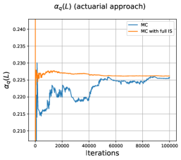
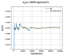
Figure 3.1: The figure shows the outcome of 100 000 iterations (number of iterations on the $x$-axis) of MC simulations with and without IS (according to Algorithm 1 in the left plot and according to Algorithm 2 in the right plot) for the computation of $\alpha_{q}(L)$ applied to a synthetic portfolio.

Input : Number $K$ of simulations

1. Determine $c$ as in (3.6);

2. Determine $\mu$ as in (3.8);

for $k=1,\dots,K$ do

      

1. Generate $X^{(k)}\sim\mathcal{N}(\mu,1)$ and determine $t(c,X^{(k)})$ as in equation (3.6);

2. Generate ${\rm LGD}_{n}^{(k)}$ according to a Beta-distribution with mean $\operatorname{ELGD}_{n}$ and variance $\nu\cdot\operatorname{ELGD}_{n}\cdot(1-\operatorname{ELGD}_{n})$ for $n=1,\dots,N$;

3. Generate a realization of $(Z_{1}^{(k)},\ldots,Z_{N}^{(k)})$ with defaults conditionally independent given $X^{(k)}$ and state $s$ probabilities of borrower $n$ given by

   $$\frac{\exp(-ta_{n}\frac{P_{nT}(s)}{P_{n0}})\pi_{ns}(X^{(k)})}{\sum_{s=1}^{S}e^{-ta_{n}\frac{P_{nT}(s)}{P_{n0}}}\pi_{ns}(X^{(k)})};$$

4. Calculate the portfolio loss

   $$L^{(k)}=-\sum_{n=1}^{N}a_{n}\sum_{s=1}^{S}\frac{P_{nT}(s)}{P_{n0}}Z_{n}^{(k)}(s)$$

end for

1. Sort the values $(L^{(k)})_{k=1,\dots,K}$ in increasing order and obtain $(L^{(k_{j})})_{j=1,\dots,K}$ ;

2. Determine $i^{*}=\inf\left\{i\in\mathbb{N}~{}|~{}\sum_{j=1}^{i}\left(M_{L|X^{(k_{j})}}(t)\cdot r_{\mu(X^{(k_{j})})}\cdot e^{-tL^{(k_{j})}}\right)\cdot L^{(k_{j})}\geq q\cdot K\right\}$ with $r_{\mu(X^{(k)})}=\exp(-\mu X^{(k)}+\frac{1}{2}\mu^{2});$

Output : Return estimator $L^{(k_{i^{*}})}$ of $\alpha_{q}(L)$;

     

Algorithm 2 IS algorithm for ratings-based CreditMetrics model.

4 Deep Learning Name Concentration Risk

Calculating the expressions (2.12), resp. (2.4), via MC simulation is computationally expensive even when using IS methods, since we are interested in very high quantiles $q=99.9\%$ or even higher. Therefore, analytic approximations as those discussed in the Appendix A have been intensively studied in the literature. These approaches perform well for commercial bank portfolios which even for small portfolios contain enough obligors so that the approximation error is sufficiently small. However, when portfolios are very small with less than 100 borrowers, these method can substantially overestimate the exposure to name concentration risk as documented by our numerical results in Section 5 and the recent study in Lütkebohmert et al. (2023).

Therefore, in this section, we suggest a NN-based based approach to compute the GAs for both the actuarial setting as well as the MtM setting. We train our network specifically for small portfolios using exact GA computations derived via MC simulations with IS. Our results document a very accurate out-of-sample performance of our NN-based GA. To learn the relation between input portfolios and the associated GA, we use function approximations in terms of NNs. Following the presentations in Lütkebohmert et al. (2022) and Goodfellow et al. (2016), we defined a (feed-forward) neural network with input dimension $d_{\operatorname{in}}\in\mathbb{N}$, output dimension $d_{\operatorname{out}}\in\mathbb{N}$, $l\in\mathbb{N}$ layers, and non-constant activation function $\varphi:\mathbb{R}\rightarrow\mathbb{R}$ as a function of the form

$$\mathbb{R}^{d_{\operatorname{in}}} \rightarrow\mathbb{R}^{d_{\operatorname{out}}}$$

$$x \mapsto A_{l}\circ\varphi\circ A_{l-1}\circ\dots\circ\varphi\circ A_{0}(x),$$

where $(A_{i})_{i=0,\dots,l}$ are affine functions $A_{i}:\mathbb{R}^{h_{i}}\rightarrow\mathbb{R}^{h_{i+1}}$, and where the activation function is applied component-wise. The number $h_{i}\in\mathbb{N}$ is called the number of neurons of layer $i$. We denote the class of all NNs with input dimension $d_{\operatorname{in}}$, output dimension $d_{\operatorname{out}}$, and with an arbitrary number of layers by $\mathfrak{N}^{\varphi}_{d_{\operatorname{in}},d_{\operatorname{out}}}$. One of the crucial properties of NNs justifying its use for function approximation is its universal approximation property, see, e.g. (Hornik, 1991, Theorem 2) or Pinkus (1999).

Lemma 4.1 (Universal Approximation Theorem)

Let the activation function $\varphi$ be continuous and non-polynomial. Then, for any compact set $\mathbb{K}\subset\mathbb{R}^{d_{\operatorname{in}}}$ the set $\mathfrak{N}_{d_{\operatorname{in}},{d_{\operatorname{out}}}}^{\varphi}|_{\mathbb{K}}$ is dense in ${C}(\mathbb{K},\mathbb{R}^{d_{\operatorname{out}}})$ with respect to the topology of uniform convergence on $C(\mathbb{K},\mathbb{R}^{d_{\operatorname{out}}})$.

4.1 NN-Based GA for Actuarial Approach

We observe that the granularity adjustment $GA_{q}^{\rm exact}(L)$ in (2.4) can be approximated arbitrarily well by NNs whenever we restrict the inputs to a compact set. The inputs consist of the exposure shares $a_{n}$, the unconditional default probabilities $\operatorname{PD}_{n}$, the expected loss given defaults $\operatorname{ELGD}_{n}$, and the sensitivities $\omega_{n}$ to the systematic risk factor for each obligor $n=1,\ldots,N$. Since restricting the inputs $(a_{n},\operatorname{PD}_{n},\operatorname{ELGD}_{n},\omega_{n})$ for $n=1,\ldots,N$ to a compact set is natural, the presented approach provides a tractable alternative to other computationally more demanding or less accurate approaches.

Lemma 4.2 (Universal Approximation)

Assume $\xi>0$ and $\nu>0$. Then, for all $q\in(0,1)$, for all $\varepsilon>0$, ${N}\in\mathbb{N}$, and all compact sets $\mathbb{K}\subset\mathbb{R}^{4{N}}$, there exists a fully connected feedforward neural network $\mathcal{N}\mathcal{N}\in\mathfrak{N}^{\varphi}_{4N,1}$, with activation function $\varphi(x)=\max\{x,0\}$ such that for all $(a,\operatorname{PD},\operatorname{ELGD},\omega)\in\mathbb{K}$ we have

$$\Bigg{|}\mathcal{N\mathcal{N}}\left(a,\operatorname{PD},\operatorname{ELGD},\omega\right)-GA_{q}^{\rm exact,act}(L)\Bigg{|}<\varepsilon.$$ (4.1)

Proof: Let $q\in(0,1)$, $\varepsilon>0$, ${N}\in\mathbb{N}$, and consider some compact set $\mathbb{K}\subset\mathbb{R}^{4{N}}$. Let $Y:=(a,{\rm PD},{\rm ELGD},\omega)=(a_{n},{\rm PD}_{n},{\rm ELGD}_{n},\omega_{n})_{n=1,\dots,N}\in\mathbb{K}$. Then, we define the (random) loss depending on $Y$ by

$$L(Y):=\sum_{n=1}^{N}a_{n}{\rm LGD}_{n}D_{n},$$

where $D_{n}$ and ${\rm LGD}_{n}$ are as defined in Section 2.1. According to the decomposition outlined in (2.4), we have

$$GA^{\rm exact,act}_{q}(L(Y)) =\alpha_{q}\left(L(Y)\right)-\sum_{n=1}^{N}a_{n}{\rm ELGD}_{n}{\rm PD}_{n}(1+\omega_{n}(\alpha_{q}(X)-1)),$$ (4.2)

where $X$ is Gamma-distributed with mean 1 and variance $1/\xi$ for some $\xi>0$. Hence, the second summand of (4.2) depends continuously on $Y$. To see that the first summand $\alpha_{q}\left(L(Y)\right)$ also depends continuously on $Y$, we aim at applying Lemma B.1. To that end, we denote by $f_{X}$ the density function of $X$ and compute for $\ell\in\mathbb{R}$:

$$\mathbb{P}\left(L(Y)\leq\ell\right)$$

$$= \sum_{(d_{1},\dots,d_{N})\in\{0,1\}^{N}}\mathbb{P}\left(L(Y)\leq\ell~{}|~{}D_{1}=d_{1},\dots,D_{N}=d_{N}\right)\cdot\mathbb{P}(D_{1}=d_{1},\dots,D_{N}=d_{N})$$

$$=\sum_{(d_{1},\dots,d_{N})\in\{0,1\}^{N}}\bigg{(}\mathbb{P}\left(L(Y)\leq\ell~{}|~{}D_{1}=d_{1},\dots,D_{N}=d_{N}\right)$$

$$\hskip 85.35826pt\times\int_{\mathbb{R}}\prod_{n=1}^{N}\mathbb{P}\left(D_{n}=d_{n}~{}\middle|~{}X=x\right)f_{X}(x)dx\bigg{)}$$

$$=\sum_{(d_{1},\dots,d_{N})\in\{0,1\}^{N}}\bigg{(}\mathbb{P}\left(L(Y)\leq\ell~{}|~{}D_{1}=d_{1},\dots,D_{N}=d_{N}\right)$$ (4.3)

$$\hskip 56.9055pt\times\int_{\mathbb{R}}\prod_{n=1}^{N}\left({\rm PD}_{n}(1+\omega_{n})(x-1)\right)^{d_{n}}\left(1-{\rm PD}_{n}(1+\omega_{n}(x-1)\right)^{1-d_{n}}f_{X}(x)dx\bigg{)}.$$

Then, note that, since $\nu>0$ (i.e. ${\rm LGD}_{i}$ is non-constant) we have that

$$\mathbb{K}\times\mathbb{R}\ni(Y,\ell)\mapsto\mathbb{P}\left(L(Y)\leq\ell~{}|~{}D_{1}=d_{1},\dots,D_{N}=d_{n}\right)$$

is continuous as the cdf of a scaled sum of independent Beta distributions. Hence, the representation in (4.3) implies that $\mathbb{K}\times\mathbb{R}\ni(Y,\ell)\mapsto\mathbb{P}\left(L(Y)\leq\ell\right)$ is continuous. Moreover, $P(L(Y)\leq\ell)$ is strictly increasing in $\ell$. Next, note that

$$\overline{\ell}:=\inf_{\ell\in\mathbb{R}}\left\{\mathbb{P}\left(L(Y)\leq\ell\right)=1\text{ for all }Y\in\mathbb{K}\right\}<\infty,$$

since the loss $L(Y)$ is bounded if we restrict $Y$ to $\mathbb{K}$. Moreover the loss $L(Y)$ is by definition non-negative. Thus, we have $\alpha_{q}(L(Y))=\inf\left\{\ell\in[0,\overline{\ell}]~{}\middle|~{}\mathbb{P}\left(L(Y)\leq\ell\right)\geq q\right\}$. By Lemma B.1 we obtain then that $\mathbb{K}\ni Y\mapsto\inf\left\{\ell\in[0,\overline{\ell}]~{}\middle|~{}\mathbb{P}\left(L(Y)\leq\ell\right)\geq q\right\}=\alpha_{q}(L(Y))$ is continuous. In particular, by (4.2), $\mathbb{K}\ni Y\mapsto GA^{\rm exact,act}_{q}(L(Y))$ is continuous. Thus, we can apply Lemma 4.1 and obtain the existence of a neural network $\mathcal{N}\mathcal{N}:\mathbb{R}^{4{N}}\rightarrow\mathbb{R}$ such that for all $Y\in\mathbb{K}$ we have

$$\Bigg{|}\mathcal{N\mathcal{N}}\left(Y\right)-GA_{q}^{\rm exact,act}(L(Y))\Bigg{|}<\varepsilon.$$ (4.4)

$\Box$

Motivated by Lemma 4.2, we present the following Algorithm 3 allowing to train NNs which are, after training, able to accurately approximate GAs for arbitrary inputs. To facilitate learning, we also include the first-order approximation of the GA (see (A.2)) as an additional input to the NN.

Input : Distributions to sample ${\rm PD},ELGD,a$ and $\omega$; Distribution to sample the number of obligors $N_{\operatorname{Obligors}}$; Maximal number of obligors $\overline{N}$; Number of iterations $N_{\operatorname{Iter}}\in\mathbb{N}$; Quantile level $q\in[0,1]$; Hyperparameters of the neural network;

Initialize the neural network $GA^{\rm NN,act}\in\mathfrak{N}^{\varphi}_{4N+1,1}$;

for $\operatorname{iteration}=1,\dots,N_{\operatorname{Iter}}$ do

       Sample the number of obligors $N_{\operatorname{Obligors}}\in\mathbb{N}$;

       Sample $a=(a_{j})_{j=1,\dots,N_{\operatorname{Obligors}}}$, $\operatorname{ELGD}=(\operatorname{ELGD}_{j})_{j=1,\dots,N_{\operatorname{Obligors}}}$, $\operatorname{PD}=(\operatorname{PD}_{j})_{j=1,\dots,N_{\operatorname{Obligors}}}$;, $\omega=(\omega_{j})_{j=1,\dots,N_{\operatorname{Obligors}}}$;

       Compute the quantile loss $Q^{L}$ according to Algorithm 1;

       Compute the conditional loss $C^{L}=\sum_{n=1}^{N}a_{n}{\rm ELGD}_{n}\pi_{n}(\alpha_{q}(X))$;

       Compute the granularity adjustment $GA=Q^{L}-C^{L}\in\mathbb{R}$;

       Compute $GA^{\rm 1st,act}$ as in (A.2);

       Minimize

$$\bigg{(}GA^{\rm NN,act}\left(\widetilde{a},\widetilde{\operatorname{PD}},\widetilde{\operatorname{ELGD}},\widetilde{\omega},GA^{\rm 1st,act}\right)-GA\bigg{)}^{2}$$

with the backpropagation algorithm, where $\widetilde{a}=\left(\left(a_{j}\right)_{j=1,\dots,N_{\operatorname{Obligors}}},0,\cdots,0\right)\in\mathbb{R}^{\overline{N}}$, $\widetilde{\operatorname{PD}}=\left(\left({\operatorname{PD}}_{j}\right)_{j=1,\dots,N_{\operatorname{Obligors}}},0,\cdots,0\right)\in\mathbb{R}^{\overline{N}}$, $\widetilde{\operatorname{ELGD}}=\left(\left({\operatorname{ELGD}}_{j}\right)_{j=1,\dots,N_{\operatorname{Obligors}}},0,\cdots,0\right)\in\mathbb{R}^{\overline{N}}$, $\widetilde{\omega}=\left(\left(\omega_{j}\right)_{j=1,\dots,N_{\operatorname{Obligors}}},0,\cdots,0\right)\in\mathbb{R}^{\overline{N}}$ ;

end for

Output : Neural network $GA^{\rm NN,act}$;

Algorithm 3 Training of a NN for the GA in the actuarial approach

4.1.1 Training

We train, according to Algorithm 3, a NN with the following specifications. The variance parameter of the Gamma distributed systematic risk factor $X$ equals $\xi=0.25$, the number of simulations $N_{\operatorname{Sim}}=1~{}000~{}000$, the number of iterations $N_{\operatorname{Iter}}=10~{}000$. We consider a feedforward NN with $5$ layers and $512$ neurons in each layer and with ReLu activation functions in each layer.

The choice of the distributions from which the input parameters are sampled for the training of the NN depends of course on the concrete application. In Section 5.2 we apply our NN-based GA to portfolios of MDBs. Therefore, we train the NN using parameter distributions that are representative for a broad range of MDB portfolios. To this end, we build on recent work in Lütkebohmert et al. (2023) who construct realistic MDB portfolios based on publicly available data in MDBs’ financial statements. The resulting portfolios all have less than 100 borrowers. Therefore, to train our NN, we set $\overline{N}=100$ and sample in each iteration

$$N_{\operatorname{Obligors}}\sim\mathcal{U}(\{10,\dots,100\}).$$

Further, for each $n=1,\dots,\overline{N}$, we sample

$$\operatorname{PD}_{n}\in\{ 0.0,0.01,0.0002,0.0004,0.0006,0.0011,$$

$$0.0018,0.004,0.009,0.0146,0.0238,0.0759,0.5147\},$$

which are the default probabilities of the S&P transition matrix from Table 5.1. We sample these $\operatorname{PD}$s with respective probabilities $0.00049$, $0.02297$, $0.00881$, $0.02627$, $0.06454$, $0.05865$, $0.06928$, $0.03111$, $0.11070$, $0.07672$, $0.19922$, $0.10282$, $0.22834,$ which are based on the empirical distribution of obligors in MDB portfolios; compare Lütkebohmert et al. (2023). The exposure distribution in each MDB portfolio can be approximated by an exponential distribution. Therefore, we sample the exposures in our training portfolios from exponential distributions with different parameters, i.e.,

$$\operatorname{EAD}_{n} \sim\operatorname{Exp}(\theta)\text{ with }\theta\sim\mathcal{U}([4,30]).~{}$$ (4.5)

$$a_{n}: =\operatorname{EAD}_{n}/\sum_{j=1}^{\overline{N}}\operatorname{EAD}_{j},$$

Moreover, we sample the factor weights according to $\omega_{n}\sim\mathcal{U}([0,1])$. Since we do not have any information on the borrower specific LGDs, in each iteration we set ${\rm ELGD}=45\%$ or ${\rm ELGD}=10\%$ for training the network. The volatility parameter $\nu$ for the LGDs is set to $0.25$ in both cases. The constant-size $400$-dimensional input vector $(a,\operatorname{PD},\operatorname{ELGD},\omega)$ to the neural network is then constructed by zero-padding, i.e., all entries $\operatorname{ELGD}_{n},a_{n},{\rm PD}_{n},\omega_{n}$ are $0$ for $n=N_{\operatorname{Obligors}}+1,\dots,100$.

4.1.2 Accuracy of the Neural Network

To test the approximation accuracy of the proposed NN approach, we compare the output of the NN-based GA with the first order approximation from (A.2) as well as with the outcome of MC simulations with $1~{}000~{}000$ simulations. To this end, we sample $1000$ input vectors according to the procedure described in Section 4.1.1. For each of the inputs we compute the GA according to each of the three approaches. Note that in the asymptotic GA, we use the same factor loadings $\omega_{n}$ for the calculation of the UL capital $\mathcal{K}_{n}$ as in the two other approaches, i.e., we implicitly set the factor loadings such that the UL capital in the CreditRisk⁺ setting and the IRB approach are identical. The confidence level is set to $q=0.999$. Our results are summarized in Table 4.1 and Figure 4.1 and indicate a much smaller prediction error for the NN-based GA than for the first order GA approximation with mean error being about 9 times larger for the latter. In Table 4.2, we only consider those portfolios with less than $25$ obligors. Here the prediction error is more than 11 times larger for $GA^{\rm 1st,act}$ than for $GA^{\rm NN,act}$. This documents that the NN approach clearly outperforms the approximation from (A.2) in terms of approximation error and shows the importance of carefully selecting the correct method to compute GAs in small portfolios.

	$|GA^{\rm NN,act}-GA^{\rm MC,act}|$	$|GA^{\rm 1st,act}-GA^{\rm MC,act}|$
No. of Portfolios	1000	1000
mean	0.00565	0.04897
std	0.00756	0.06346
min	0.00000	0.00020
25%	0.00162	0.01696
50%	0.00351	0.02814
75%	0.00658	0.05463
max	0.08046	0.82322

Table 4.1: Actuarial Approach: The table shows the approximation error of the NN-based $GA^{\rm NN,act}$ and the first order approximation $GA^{\rm 1st,act}$ from (A.2) when compared with $GA^{\rm MC,act}$ computed by MC simulation with $10^{6}$ simulations of the underlying risk factor. We tested the approaches on $1000$ inputs that were sampled according to the distributions indicated Section 4.1.1. The considered confidence level is $q=0.999$.

	$|GA^{\rm NN,act}-GA^{\rm MC,act}|$	$|GA^{\rm 1st,act}-GA^{\rm MC,act}|$
No. of Portfolios	166	166
mean	0.01275	0.13860
std	0.01393	0.10879
min	0.00002	0.00446
25%	0.00295	0.07441
50%	0.00748	0.10433
75%	0.01818	0.16566
max	0.08046	0.82322

Table 4.2: Actuarial Approach: The table shows the approximation error of the NN-based $GA^{\rm NN,act}$ and the first order approximation $GA^{\rm 1st,act}$ from (A.2) when compared with $GA^{\rm MC,act}$ computed by MC simulation with $10^{6}$ simulations of the underlying risk factor. We tested the approaches on $1000$ inputs that were sampled according to the distributions indicated Section 4.1.1. However, in this table we only consider those portfolios with less than $25$ obligors. The confidence level is $q=0.999$.

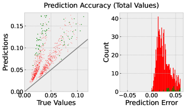
(a) First order approximation GA

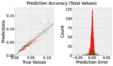
(b) NN-based GA

Figure 4.1: Actuarial Approach: This figure illustrates the accuracy of the predictions on the test set of 1000 sampled portfolios. The left panels of both subfigures (a) and (b) show a plot of all target values (x-values) generated by MC simulation and its predictions (y-values) either according to the first-order GA approximation from (A.2) (a) or according to the trained NN (b). The right panels depict histograms of the corresponding prediction error, i.e., the error between target values and predicted values. The green dots correspond to portfolios with less than $25$ borrowers. The confidence level is $q=0.999$.

4.2 NN-Based GA for MtM Approach

When considering the MtM approach, the portfolio is characterized by the exposure shares $a_{n}$, the expected loss given defaults ${\rm ELGD}_{n}$, the asset correlations $\rho_{n}$, the coupons $c_{n}$, the maturities $\tau_{n}$, and the current rating $g_{n}$ of each obligor $n=1,\ldots,N$. To compute the GA, we derive the following universal approximation result allowing to approximate the GA from (2.12) by NNs.

Lemma 4.3 (Universal Approximation)

Let $\mathbb{G}\subset\mathbb{N}$ and $\mathbb{T}\subset\mathbb{N}$ be finite sets. For all $q\in(0,1)$, for all $\varepsilon>0$, $\nu>0$, number of obligors ${N}\in\mathbb{N}$, number of states $S\in\mathbb{N}$, transition probabilities $(p_{ss^{\prime}})_{s=1,\dots,S\atop s^{\prime}=0,\dots,S}$ and compact sets $\mathbb{K}\subset\mathbb{R}^{4\overline{N}}$, there exists a fully connected feedforward neural network $\mathcal{N}\mathcal{N}\in\mathfrak{N}^{\varphi}_{6N,1}$, with $\varphi(x)=\max\{x,0\}$ such that for all $(a,\operatorname{ELGD},\rho,c,g,\tau)\in\mathbb{K}\times\mathbb{G}^{N}\times\mathbb{T}^{N}$ we have

$$\Bigg{|}\mathcal{N\mathcal{N}}\left((a,\operatorname{ELGD},\rho,c,g,\tau)\right)-GA_{q}^{\rm exact,MtM}(L)\Bigg{|}<\varepsilon.$$ (4.6)

Proof: Let $q\in(0,1)$, $\varepsilon>0$, ${N}\in\mathbb{N}$, and consider some compact set $\mathbb{K}\subset\mathbb{R}^{4{N}}$. We pick some $(g,\tau)\in\mathbb{G}^{N}\times\mathbb{T}^{N}$ and some $Y:=(a,\operatorname{ELGD},\rho,c)\in\mathbb{R}^{4{N}}$. Then, we define the loss in dependence of $Y$, $g$, and $\tau$ by

$$L(Y,g,\tau):=-\sum_{n=1}^{N}a_{n}\sum_{s=1}^{S}\frac{P_{nT}(s)}{P_{n0}}\cdot\mathds{1}_{\left\{\Phi^{-1}\left(\sum_{i=0}^{s-1}p_{g(n),i}\right)<~{}Y_{n}~{}\leq\Phi^{-1}\left(\sum_{i=0}^{s}p_{g(n),i}\right)\right\}},$$

where the transition probabilities $p_{g(n),i}$ only depend on the rating $g(n)$ of each obligor $n$. According to (2.12) we have

$$GA^{\rm exact,MtM}_{q}(L(Y,g,\tau))=\alpha_{q}(L(Y,g,\tau))-\mathbb{E}[L(Y,g,\tau)~{}|~{}\alpha_{1-q}(X)],$$ (4.7)

where it can be easily seen that the second summand of (4.7)

$$\begin{array}[]{ccl}\mathbb{E}[L(Y,g,\tau)~{}|~{}\alpha_{1-q}(X)]&=&\displaystyle e^{-rT}\sum_{n=1}^{N}a_{n}\cdot\mu_{n}(\alpha_{1-q}(X))\\[5.69054pt] &=&\displaystyle e^{-rT}\sum_{n=1}^{N}a_{n}\cdot\sum_{s=0}^{S}\mathbb{E}[R_{n}|S_{n}=s]\pi_{ns}(\alpha_{1-q}(X))\end{array}$$

depends continuously on $Y=(a,\operatorname{ELGD},\rho,c)$. Here, $R_{n}$ is defined by (2.11) and $\pi_{ns}(X)$ is given by (2.6). We denote by $f_{X}$ the density of a standard normal distribution and obtain for all $\ell\in\mathbb{R}$ that

$$\mathbb{P}\left(L(Y,g,\tau)\leq l\right) =\sum_{(s_{1},\dots,s_{N})\in\{1,\dots,S\}^{N}}\bigg{(}\mathbb{P}\left(L(Y,g,\tau)\leq\ell~{}\middle|~{}S_{1}=s_{1},\dots,S_{N}=s_{N}\right)$$

$$\hskip 113.81102pt\times\mathbb{P}\left(S_{1}=s_{1},\dots,S_{N}=s_{N}\right)\bigg{)}$$

$$=\sum_{(s_{1},\dots,s_{N})\in\{1,\dots,S\}^{N}}\bigg{(}\mathbb{P}\left(L(Y,g,\tau)\leq\ell~{}\middle|~{}S_{1}=s_{1},\dots,S_{N}=s_{N}\right)$$

$$\hskip 113.81102pt\times\int_{\mathbb{R}}\prod_{n=1}^{N}\pi_{ns}(x)f_{X}(x)dx\bigg{)}$$

which depends continuously on $Y$ and $\ell$ as $\nu>0$, and is strictly increasing in $\ell$. Note further that

$$\overline{\ell}:=\inf_{\ell\in\mathbb{R}}\left\{\mathbb{P}\left(L(Y,g,\tau)\leq\ell\right)=1\text{ for all }Y\in\mathbb{K}\right\}<\infty,$$

since the loss $L(Y,g,\tau)$ is bounded if we restrict $Y$ to $\mathbb{K}$. Moreover, $-L(Y,g,\tau)$ is by definition non-negative. Thus, we have

$$\alpha_{q}(L(Y,g,\tau))=-\alpha_{1-q}(-L(Y,g,\tau))=-\inf\left\{\ell\in[0,\overline{\ell}]~{}\middle|~{}\mathbb{P}\left(-L(Y,g,\tau)\leq\ell\right)\geq 1-q\right\}$$

for some $\overline{\ell}>0$. Due to Lemma B.1, we then obtain that $\mathbb{K}\ni Y\mapsto\alpha_{q}(L(Y,g,\tau))$ is continuous and thus, by (4.7), also $\mathbb{K}\ni Y\mapsto GA^{\rm exact,MtM}_{q}(L(Y,g,\tau))$ is continuous.

Applying linear interpolation on the grid $\mathbb{G}\times\mathbb{T}$, we may then conclude the existence of a continuous function

$$\mathbb{R}^{4N}\times\mathbb{R}\times\mathbb{R}\ni(Y,g,\tau)\mapsto\Psi(Y,g,\tau)\text{ s.t. }\Psi(Y,g,\tau)|_{\mathbb{K}\times\mathbb{G}\times\mathbb{T}}=GA^{\rm exact,MtM}_{q}(L(Y,g,\tau)).$$

Eventually, we apply Lemma 4.1 to $\Psi$ and obtain the existence of a neural network $\mathcal{N}\mathcal{N}:\mathbb{R}^{6{N}}\rightarrow\mathbb{R}$ such that for all $(Y,g,\tau)\in\mathbb{K}\times\mathbb{G}\times\mathbb{T}$ we have

$$\Bigg{|}\mathcal{N}\mathcal{N}\left(Y,g,\tau\right)-\Psi(L(Y,g,\tau))\Bigg{|}=\Bigg{|}\mathcal{N}\mathcal{N}\left(Y,g,\tau\right)-GA^{\rm exact,MtM}_{q}(L(Y,g,\tau))\Bigg{|}<\varepsilon.$$ (4.8)

$\Box$

In the MtM setting, Algorithm 4 allows to train NNs which are then able to compute GAs for any input of portfolio parameters. To improve learning and in line with the approach for the actuarial case, we include the first-order approximation $GA^{\rm 1st,MtM}$ in (A.3) as an additional input to the neural network.

Input : Distributions to sample ${\rm ELGD},a,\rho,c,\tau,g$; Distribution to sample the number of obligors $N_{\operatorname{Obligors}}$; Transition Matrix $(p_{s,s,})_{s,s^{\prime}=0,\dots,S}$; Maximal number of obligors $\overline{N}$; Number of iterations $N_{\operatorname{Iter}}\in\mathbb{N}$; Quantile level $q\in[0,1]$;

Initialize the neural network $GA^{\rm NN,MtM}\in\mathfrak{N}^{\varphi}_{6N+1,1}$;

for $\operatorname{iteration}=1,\dots,N_{\operatorname{Iter}}$ do

       Sample number of obligors $N_{\operatorname{Obligors}}\in\mathbb{N}$;

       Sample $a=(a_{j})_{j=1,\dots,N_{\operatorname{Obligors}}}$, $\operatorname{ELGD}=(\operatorname{ELGD}_{j})_{j=1,\dots,N_{\operatorname{Obligors}}}$, $\rho=(\rho_{j})_{j=1,\dots,N_{\operatorname{Obligors}}}$, $\operatorname{c}=(\operatorname{c}_{j})_{j=1,\dots,N_{\operatorname{Obligors}}}$, $(g_{j})_{j=1,\dots,N_{\operatorname{Obligors}}}$, and $\tau=(\operatorname{\tau}_{j})_{j=1,\dots,N_{\operatorname{Obligors}}}$;

       Compute the quantile loss $Q^{L}$ with Algorithm 2;

       Compute the conditional loss $C^{L}=-\sum_{n=1}^{N}a_{n}\cdot\mu_{n}(\alpha_{1-q}(X))$;

       Compute the granularity adjustment $GA=e^{-rT}\left(Q^{L}-C^{L}\right)\in\mathbb{R}$;

       Compute $GA^{\rm 1st,MtM}$ as in (A.3);

       Minimize

$$\bigg{(}GA^{\rm NN,MtM}\left(\widetilde{a},\widetilde{\operatorname{ELGD}},\widetilde{\rho},\widetilde{\operatorname{c}},\widetilde{g},\widetilde{\tau},GA^{\rm 1st,MtM}\right)-GA\bigg{)}^{2}$$

with the backpropagation algorithm, where $\widetilde{a}=\left(\left(a_{j}\right)_{j=1,\dots,N_{\operatorname{Obligors}}},0,\cdots,0\right)\in\mathbb{R}^{\overline{N}}$, $\widetilde{\operatorname{ELGD}}=\left(\left({\operatorname{ELGD}}_{j}\right)_{j=1,\dots,N_{\operatorname{Obligors}}},0,\cdots,0\right)\in\mathbb{R}^{\overline{N}}$, $\widetilde{\rho}=\left(\left(\rho_{j}\right)_{j=1,\dots,N_{\operatorname{Obligors}}},0,\cdots,0\right)\in\mathbb{R}^{\overline{N}}$ , $\widetilde{\operatorname{c}}=\left(\left({\operatorname{c}}_{j}\right)_{j=1,\dots,N_{\operatorname{Obligors}}},0,\cdots,0\right)\in\mathbb{R}^{\overline{N}}$, $\widetilde{\operatorname{g}}=\left(\left({\operatorname{g}}_{j}\right)_{j=1,\dots,N_{\operatorname{Obligors}}},0,\cdots,0\right)\in\mathbb{R}^{\overline{N}}$, $\widetilde{\tau}=\left(\left({\tau}_{j}\right)_{j=1,\dots,N_{\operatorname{Obligors}}},0,\cdots,0\right)\in\mathbb{R}^{\overline{N}}$;

end for

Output : Neural network $GA^{\rm NN,MtM}$;

Algorithm 4 Training of a NN for the GA in the MtM approach

4.2.1 Training

For training the NN, according to Algorithm 4, we consider similar specifications as for the actuarial case, i.e. the number of simulations $N_{\operatorname{Sim}}=1~{}000~{}000$, the number of iterations $N_{\operatorname{Iter}}=10~{}000$. The neural network is a feedforward neural network with $5$ layers and $512$ neurons in each layer where a ReLu activation function is applied to each layer.

To train the NN, we set $\overline{N}=100$ and we sample in each iteration

$$N_{\operatorname{Obligors}}\sim\mathcal{U}(\{10,\dots,100\}).$$

Similarly to Section 4.1.1, for $n=1,\dots,\overline{N}$ we sample the exposures from an exponential distribution. Further parameters are sample according to uniform distributions, i.e.,

$$\operatorname{EAD}_{n} \sim\operatorname{Exp}(\theta)\text{ with }\theta\sim\mathcal{U}([4,30]),~{}$$ (4.9)

$$a_{n}: =\operatorname{EAD}_{n}/\sum_{j=1}^{\overline{N}}\operatorname{EAD}_{j},$$

$$\rho_{n} \sim\mathcal{U}([0.15,0.7]),~{}$$

$$c_{n} \sim\mathcal{U}([0,0.1])$$

$$D_{n} \sim\mathcal{U}([1,10]),~{}$$

The range of the asset correlation parameters stems from the empirical study in Lütkebohmert et al. (2023). Since there is no publicly available information on coupon rates, we sample these from a rather wide range of values. According to Lütkebohmert et al. (2023) maturities of sovereign loans range between a few months and up to 35 years with the majority of loans maturing within the next 10 years, and are mostly uniformly distributed over this time period. Therefore, to facilitate training, we assume maturities are uniformly distributed between one and ten years. We sample the initial ratings $g_{n}$ (analogous to the PDs in the actuarial case) from the probabilities implied by the S&P transition matrix from Table 5.1 and the overall empirical distribution of obligors in MDB portfolios described in Lütkebohmert et al. (2023). The rating transition matrix in Table 5.1 is also used for training the NN approach in the MtM setting. Thus, we consider 17 non-default states and an absorbing default state. Similarly as before, we set ${\rm ELGD}=45\%$ or ${\rm ELGD}=10\%$ and the volatility parameter $\nu=0.25$ for training the network. The constant-size $600$-dimensional input vector $(a,\operatorname{ELGD},\rho,c,g,D)$ to the NN is then constructed by zero-padding, i.e., all entries $a_{n},\operatorname{ELGD}_{n},\rho_{n},c_{n},g_{n},D_{n}$ are $0$ for $n=N_{\operatorname{Obligors}}+1,\dots,100$.

4.2.2 Accuracy of the Neural Network

We compare the output of the NN-based GA and the first order approximation from (A.3) with GA computations based on MC simulations with $1~{}000~{}000$ simulations. To this end, we consider $1000$ different input vectors, which are sampled according to the procedure outlined in Section 4.2.1. For each of the inputs, we compute the GA according to each of the three approaches for the confidence level $q=0.999$. Results are summarized in Table 4.3 and Figure 4.2. As can be observed, the prediction error for the first order GA approximation from (A.3) is on average about twice as large as for the NN-based GA. This documents that the NN GA significantly outperforms the analytic GA with respect to the approximation error. When considering only the very small portfolios with less than 25 obligors as shown in Table 4.4, the effect is comparable. Overall, the results show that even for high quantiles as $q=0.999$ the NN can be efficiently trained to accurately predict the GA for small and concentrated portfolios.

(a) Girst order approximation GA

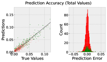
(b) NN-based GA

Figure 4.2: MtM approach: This figure illustrates the accuracy of the predictions on the test set of 1000 sampled portfolios. The left panels of both subfigure (a) and (b) show a plot of all target values (x-values) generated by MC simulation and its predictions (y-values) either according to the first order GA approximation from (A.3) (a) or according to the trained NN (b). The right panels depict histograms of the corresponding prediction error, i.e., the error between target values and predicted values. The green dots correspond to portfolios with less than $25$ borrowers. The confidence level is $q=0.999$.

	$|GA^{\rm NN,MtM}-GA^{\rm MC,MtM}|$	$|GA^{\rm 1st,MtM}-GA^{\rm MC,MtM}|$
No. of Portfolios	1000	1000
mean	0.00573	0.01084
std	0.00586	0.00917
min	0.00003	0.00004
25%	0.00201	0.00397
50%	0.00416	0.00892
75%	0.00753	0.01509
max	0.06398	0.08030

Table 4.3: MtM approach: The table shows the approximation error of the NN-based $GA^{\rm NN,MtM}$ and the first order approximation $GA^{\rm 1st,MtM}$ from (A.3) when compared to $GA^{\rm MC,MtM}$ computed by MC simulation with $10^{6}$ simulations of the underlying risk factor. We tested the approaches on $1000$ inputs that were sampled according to the distributions indicated in Section 4.2.1. The confidence level is $q=0.999$.

	$|GA^{\rm NN,MtM}-GA^{\rm MC,MtM}|$	$|GA^{\rm 1st,MtM}-GA^{\rm MC,MtM}|$
No. of Portfolios	184	184
mean	0.00882	0.01500
std	0.00932	0.01310
min	0.00003	0.00009
25%	0.00257	0.00512
50%	0.00645	0.01228
75%	0.01181	0.02098
max	0.06398	0.08030

Table 4.4: Mtm approach: The table shows the approximation error of the NN-based $GA^{\rm NN,MtM}$ and the first order approximation $GA^{\rm 1st,MtM}$ from (A.3) when compared to $GA^{\rm MC,MtM}$ computed by MC simulation with $10^{6}$ simulations of the underlying risk factor. We tested the approaches on $1000$ inputs that were sampled according to the distributions indicated in Section 4.2.1, however in this figure, we only consider those portfolios with less than $25$ obligors. The confidence level is $q=0.999$.

5 Performance Evaluation of the NN Approach

5.1 Sensitivity Analysis based on Simulated Portfolios

In this section, we study the impact of different input parameters on the size of the GA. To this end, we sample a portfolio with $100$ obligors with input parameters distributed as described in Sections 4.1.1 and 4.2.1 for the actuarial approach and the MtM approach, respectively. First we investigate the effect of reducing the number of obligors by gradually deleting obligors from the originally sampled portfolio, depicted in Figure 5.1 (a) for the actuarial and in Figure 5.2 (a) for the MtM approach. We observe that with an increasing number of obligors the GA tends to decrease while this relation is not necessarily monotone since adding single obligors with large exposure or high PDs might also increase the GA as can be clearly observed in the MtM case. Figure 5.1 (a) further shows that the approximate GA in the actuarial approach overestimates the true GA (approximated by the NN) significantly which is also in line with the results in Figure 4.1. In the MtM approach, it highly depends on the choice of the portfolio whether the approx. GA over- or underestimates the true GA with overestimation occurring more frequently than underestimations (compare Figure 5.2 (a) and also Figure 4.2).

Next, we study the impact of varying the credit quality or the relative weights of individual loans in the portfolio on the $GA$. Therefore, to consider an average-sized portfolio, we construct a portfolio consisting of only $50$ obligors sampled according to our input distributions for the actuarial and the MtM case. We depict the composition of these portfolios ordered by an increasing exposure share together with the assigned ${\rm PD}$ in Figures 5.1 (b) and  5.2 (b), respectively.

To study the effect of a change in the credit quality of an individual borrower on the name concentration risk of the credit portfolio, we consider a single notch downgrade for each of the obligors in the respective portfolios. It can be observed that the effect on the GA is the more pronounced the larger the exposure of the respective obligor is, i.e., if a borrower with a large relative weight gets downgraded, this increases the name concentration of the portfolio and therefore leads to a rising GA. The opposite effect occurs when the rating of the borrower improves. We show these effects in Figure 5.1 (c) and  5.2 (c).

Finally, we investigate the influence of increasing the relative portfolio weight (given by $a_{i}=\operatorname{EAD}_{i}/\sum_{j=1}^{50}\operatorname{EAD}_{j}$) of a single obligor by $1\%$. The extent to which this change in the portfolio composition affects the GA depends crucially on both the relative portfolio weight of the respective obligor and its PD, whereby the influence of the relative portfolio weight appears to be stronger: If the relative portfolio weight before the increase is rather low, the effect of the $1\%$ increase is usually a reduction in the GA, as the portfolios becomes more homogeneous so that name concentration is reduced. However, if the relative weight is already high, then a further increase in the weight increases also the name concentration and hence the GA, unless the PD is small. In this case, an increase in the relative weight can lead to a better overall quality of the portfolio and thus to a reduction in the GA. Compare for a detailed illustration Figure 5.1 (d) and  5.2 (d).

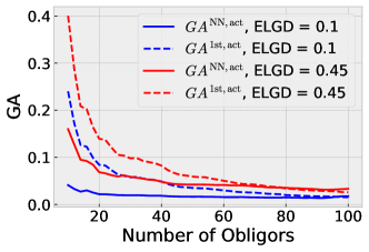
(a) Sensitivity w.r.t. number of obligors.

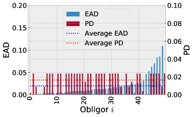
(b) Reduced Portfolio with 50 Obligors

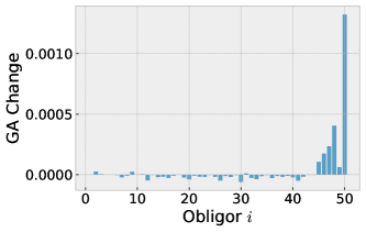
(c) Sensitivity w.r.t. 1 notch downgrade

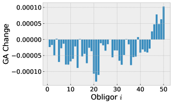
(d) Sensitivity w.r.t. 1% change in $a_{n}$

Figure 5.1: The figure shows the sensitivities of the approximate and NN GA in the actuarial approach of a portfolio sampled according to Section 4.1.1 w.r.t. the number of obligors (a). In Subfigure (b) we show the composition of a reduced portfolio of 50 obligors, which we consider in (c) to study the impact of a single notch downgrade on $GA^{\rm NN,act}$. The impact of an increase in an obligor’s exposure share $a_{n}$ on $GA^{\rm NN,act}$ is depicted in (d).

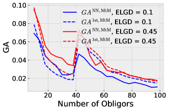
(a) Sensitivity w.r.t. number of obligors.

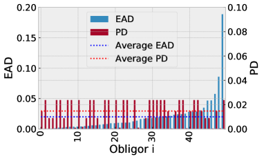
(b) Reduced Portfolio with 50 Obligors

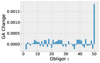
(c) Sensitivity w.r.t. 1 notch downgrade

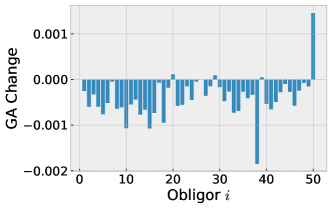
(d) Sensitivity w.r.t. 1% change in $a_{n}$

Figure 5.2: The figure shows the sensitivities of the approximate and NN GA in the MtM approach of a portfolio sampled according to Section 4.2.1 w.r.t. the number of obligors (a). In Subfigure (b) we show the composition of a reduced portfolio of 50 obligors, which we consider in (c) to study the impact of a single notch downgrade on $GA^{\rm NN,MtM}$. The impact of an increase in an obligor’s exposure share $a_{n}$ on $GA^{\rm NN,MtM}$ is depicted in (d)

Overall, these results document that the impact of changes in individual borrower’s characteristics or exposure shares on the name concentration risk of the loan portfolio is quite complex. The effect of including an additional loan to an existing portfolio is similar. Thus, quantitative tools as our proposed method are very useful to evaluate these effects. In particular, our NN-based GA allows for a fast and accurate evaluation of such sensitivities whereas comparable calculations based on MC simulations are computationally expensive. In this way, our approach can help, for instance, to examine the impact of a potential future downgrading of a borrower on the name concentration risk of the portfolio, which could be extremely useful for rating agencies, for example. Alternatively, our NN-based GA can be applied to evaluate how adding loans to a portfolio may affect the portfolio’s exposure to name concentration risk. This might be very valuable for the investment decisions of institutions if they want to maintain certain risk assessments.

5.2 Application to Realistic MDB Portfolios

Next, we evaluate the performance of our NN GA based on realistic MDB portfolios as constructed in Lütkebohmert et al. (2023) for eleven MDBs from their publicly available financial statements:

• African Development Bank (AfDB); see AfDB (2022)

• Asian Development Bank (ADB); see ADB (2022)

• Development Bank of Latin America and the Caribbean (CAF); see CAF (2022)

• Caribbean Development Bank (CDB); see CDB (2022)

• Central American Bank for Economic Integration (CABEI); see CABEI (2022)

• East African Development Bank (EADB); see EADB (2022)

• European Bank for Reconstruction and Development (EBRD); see EBRD (2022)

• Inter-American Development Bank (IDB); see IDB (2022)

• International Bank for Reconstruction and Development (IBRD); see IBRD (2022)

• Trade and Development Bank (TDB); see TDB (2022)

• West African Development Bank (BOAD); see BOAD (2022)

We consider two different values for ${\rm ELGD}$ by either setting ${\rm ELGD}=45\%$ or, to account for preferred creditor treatment (PCT), by choosing ${\rm ELGD}=10\%$ which is in line with the specification imposed by S&P for sovereign’s borrowing from MDBs with high preferred creditor status. Moreover, we set the parameter $\nu=25\%$ implying a volatility of the LGD variable of ${\rm VLGD}=0.25$ without PCT (i.e. when ${\rm ELGD}=45\%$) and ${\rm VLGD}=0.15$ with PCT (i.e. for ${\rm ELGD}=10\%$). This choice is in line with estimates of sovereign haircuts in Cruces and Trebesch (2013) when assuming the recovery rate to be beta distributed.

Since most loans to sovereign borrowers of various countries are denominated in USD, we use the average one-year foreign currency rating transition matrix estimated for the time period 1975–2021 as published in S&P Global Ratings (2022). We follow S&P Global Ratings (2017, 2018), who impose a minimal rating of B-, and in line with Risk Control (2023) we merge all ratings CCC+ and worse into a consolidated rating ‘Cs’. The resulting normalised transition matrix is reported in Table 5.1 (see also Risk Control (2023), Table A3.5). To convert these historical transition probabilities into risk-neutral transition rates, we follow Agrawal et al. (2004) and Kealhofer (2003) and assume a market Sharpe ratio of $\psi=0.4.$ Risk-neutral probabilities $p^{*}_{s}(t,T)$ are then calculated as in the KMV model by

$$p^{*}_{s}(t,T)=\Phi(\Phi^{-1}(p_{s}(t,T))+\psi\sqrt{T-t}\sqrt{\rho}),$$

where $\rho$ denotes the asset correlation. We determine the borrower-specific asset correlation parameter $\rho_{n}$ according the formula in the IRB approach (compare Basel Committee on Banking Supervision (2011), p.39) such that $\rho_{n}$ ranges between 12% and 24%.

The DL approach in the actuarial setting further requires the factor loading $\omega_{n}$ for each borrower $n$ as input, which we obtain by setting the UL capital in the IRB approach (compare Basel Committee on Banking Supervision (2011), p. 39) equal to the UL capital in the CreditRisk⁺ model (see equation (A.1)) with $x_{q}$ equal to the $q^{\rm th}$ quantile of the Gamma$(\xi,1/\xi)$-distributed risk factor $X$ for $\xi=0.25$ and then solve for $\omega_{n}$. Note that the asymptotic GA in the actuarial approach as derived in Gordy and Lütkebohmert (2013) and implemented under the S&P approach does not require this parameter as an input because it directly uses the $\mathcal{K}_{n}$ and $\mathcal{R}_{n}$ values of the IRB approach.

	AAA	AA+	AA	AA-	A+	A	A-	BBB+	BBB	BBB-	BB+	BB	BB-	B+	B	B-	Cs	D
AAA	96.79	2.71	0.42	0.00	0.00	0.00	0.01	0.00	0.00	0.00	0.00	0.07	0.00	0.00	0.00	0.00	0.00	0.00
AA+	6.45	85.16	6.61	1.77	0.00	0.00	0.00	0.00	0.00	0.00	0.00	0.00	0.00	0.00	0.00	0.00	0.00	0.00
AA	0.00	6.22	85.17	6.74	0.52	0.42	0.10	0.52	0.00	0.00	0.00	0.31	0.00	0.00	0.00	0.00	0.00	0.00
AA-	0.00	0.00	7.82	83.45	7.16	0.17	0.50	0.17	0.00	0.17	0.44	0.00	0.00	0.11	0.00	0.00	0.00	0.00
A+	0.00	0.00	0.07	13.35	73.28	9.30	2.03	1.12	0.14	0.63	0.07	0.00	0.00	0.00	0.00	0.00	0.00	0.01
A	0.00	0.00	0.00	1.15	12.33	77.29	5.71	1.68	0.77	0.96	0.10	0.00	0.00	0.00	0.00	0.00	0.00	0.01
A-	0.00	0.00	0.00	0.00	0.94	11.47	77.82	6.94	0.41	1.57	0.67	0.16	0.00	0.00	0.00	0.00	0.00	0.02
BBB+	0.00	0.00	0.00	0.00	0.00	2.16	12.39	70.86	11.24	2.41	0.60	0.24	0.06	0.00	0.00	0.00	0.00	0.04
BBB	0.00	0.00	0.00	0.00	0.00	0.00	1.87	16.60	68.05	11.16	0.99	0.11	0.00	0.50	0.22	0.11	0.33	0.06
BBB-	0.00	0.00	0.00	0.00	0.00	0.00	0.00	0.93	14.94	74.69	6.50	2.13	0.27	0.08	0.15	0.12	0.08	0.11
BB+	0.00	0.00	0.00	0.00	0.00	0.00	0.00	0.00	0.54	20.57	66.38	9.93	1.14	0.18	0.06	0.00	1.02	0.18
BB	0.00	0.00	0.00	0.00	0.00	0.00	0.00	0.00	0.00	0.78	14.20	70.80	11.15	1.80	0.68	0.15	0.05	0.40
BB-	0.00	0.00	0.00	0.00	0.00	0.00	0.00	0.00	0.00	0.00	1.03	10.55	73.79	11.47	1.19	0.46	0.61	0.90
B+	0.00	0.00	0.00	0.00	0.00	0.00	0.00	0.00	0.00	0.03	0.03	0.92	10.20	68.70	15.30	2.50	0.85	1.46
B	0.00	0.00	0.00	0.00	0.00	0.00	0.00	0.00	0.00	0.00	0.00	0.00	0.61	13.50	70.77	9.84	2.91	2.38
B-	0.00	0.00	0.00	0.00	0.00	0.00	0.00	0.00	0.00	0.00	0.00	0.00	0.00	2.43	15.07	66.85	8.05	7.59
Cs	0.00	0.00	0.00	0.00	0.00	0.00	0.00	0.00	0.00	0.00	0.00	0.00	0.00	0.74	1.81	13.90	32.08	51.47
D	0.00	0.00	0.00	0.00	0.00	0.00	0.00	0.00	0.00	0.00	0.00	0.00	0.00	0.00	0.00	0.00	0.00	100.00

Table 5.1: Normalizes average one-year sovereign foreign currency transition matrix (transition probabilities in %).

Detailed information on loan maturities is not publicly available but a rough distribution of exposures in different maturity ranges for the individual MDBs can be inferred from their financial statements and average maturities are reported Table 1 in Lütkebohmert et al. (2023). In our calculations, for simplicity, we set the maturity equal to one for all loans. Further, we impose the assumption that interest is paid semiannually in all contracts and assume that coupon rates are equal to 1%.

As risk-free interest rates used for discounting future cash flows we construct the Nelson-Siegel-Svensson curve for the US treasury rate based on the parameters published on the website of the Board of Governors of the Federal Reserve System. Since we consider financial statements as of December 31, 2022, we construct the yield curve for December 30, 2022 (last business day of the year).

We calculate the GA at a confidence level of $q=99.9\%$ over a time horizon of $T=1$ year. We compute the NN GA and the analytic approximation GA in both the actuarial CreditRisk⁺ model and the MtM approach and calculate the percentage error with respect to the exact GA obtained by MC simulations with IS.

The GAs for the described MDB portfolios are reported in Tables 5.2 and 5.3. Our results for the percentage error between the NN GA and the exact MC GA show that the NN approach is highly accurate for both the actuarial CreditRisk⁺ model and the MtM approach. Comparing the results to the percentage error of the approximate GAs documents that our NN GA clearly outperforms the respective analytical approximations. For the CreditRisk⁺ model the percentage error for the approximate GA is up to 75 times higher than the one for the NN GA for the case ${\rm ELGD}=45\%$ and even more for ${\rm ELGD}=10\%$. The approximate GA for the MtM setting is more accurate in general but still performs worse than the NN GA with a percentage error of up to 14 times higher than the one for the NN GA.

The NN GA is also highly accurate for the two very small portfolios in the sample which have less than 10 obligors. This is particularly remarkable since the NN was only trained on portfolios with at least 10 borrowers.

The out-of-sample results for the simulated portfolios in Section 4 already illustrated the superior performance of our NN GA compared to the analytic methods. The out-of-sample results based on real portfolio data in this subsection document that our NN GA is also highly accurate in real data applications, i.e. when applied to portfolios with characteristics that are not just sampled from the training distributions. The accuracy of the NN GA of course increases when the distributions used for training fit more closely to the empirical distributions of the real portfolios. While our NN was trained using parametric distributions with parameters fit to the real portfolios, training based on empirical distributions of historical portfolio data could substantially increase precision. In this way, MDBs or rating agencies that have access to such historical portfolio data, could use our methodology to obtain a highly accurate and very fast estimate for the name concentration risk in current portfolios.

	CAF	ADB	AFDB	IDB	CDB	CABEI	EADB	IBRD	TDB	BOAD	EBRD
Borrowers	16	38	29	26	16	11	4	78	21	8	37
$GA^{\rm NN,act}$	15.00	7.61	8.44	9.45	8.38	17.46	19.51	4.17	13.16	16.04	7.69
$GA^{\rm 1st,act}$	29.52	19.84	15.63	25.08	22.05	59.95	49.97	6.85	34.62	32.93	14.29
$GA^{\rm NN,MtM}$	21.13	11.88	13.07	16.18	18.02	34.73	33.66	5.32	26.71	24.50	11.34
$GA^{\rm 1st,MtM}$	23.87	13.87	12.36	17.92	19.64	44.54	42.86	5.19	31.25	27.79	10.91
$GA^{\rm MC,act}$	12.46	7.07	8.00	9.24	11.89	20.38	27.13	4.35	15.23	15.78	8.76
$GA^{\rm MC,MtM}$	18.71	10.34	12.48	13.32	18.76	25.85	36.44	6.38	25.95	22.75	11.20
Percentage Error $GA^{\rm NN,act}$	20.42	7.59	5.54	2.26	29.50	14.33	28.08	4.23	13.58	1.64	12.21
Percentage Error $GA^{\rm 1st,act}$	136.90	180.64	95.32	171.46	85.49	194.18	84.18	57.48	127.33	108.66	63.09
Percentage Error $GA^{\rm NN,MtM}$	12.91	14.93	4.71	21.49	3.97	34.37	7.63	16.68	2.94	7.71	1.21
Percentage Error $GA^{\rm 1st,MtM}$	27.56	34.13	0.93	34.52	4.69	72.32	17.62	18.58	20.42	22.16	2.62

Table 5.2: The GAs of the MDBs, described in Section 5.2, using the different approaches under the assumption that $\operatorname{ELGD}\equiv 0.45$ for all obligors.

	CAF	ADB	AFDB	IDB	CDB	CABEI	EADB	IBRD	TDB	BOAD	EBRD
Borrowers	16	38	29	26	16	11	4	78	21	8	37
$GA^{\rm NN,act}$	4.46	3.67	3.88	4.15	3.77	6.58	5.62	2.33	5.61	5.14	3.03
$GA^{\rm 1st,act}$	20.35	13.93	10.68	17.51	14.56	41.84	29.58	4.57	24.81	22.77	9.61
$GA^{\rm NN,MtM}$	15.46	8.86	8.38	12.19	12.36	25.64	20.49	3.66	22.19	18.69	6.94
$GA^{\rm 1st,MtM}$	17.93	10.63	9.03	13.61	13.62	34.11	25.42	3.60	26.85	21.42	7.59
$GA^{\rm MC,act}$	4.35	2.65	3.13	3.38	3.96	5.98	12.72	1.49	6.88	5.58	2.33
$GA^{\rm MC,MTM}$	11.58	7.78	8.09	10.19	11.72	18.88	22.12	3.74	15.98	13.39	6.84
Percentage Error $GA^{\rm NN,act}$	2.52	38.66	24.03	22.72	4.81	10.02	55.79	56.28	18.45	7.95	29.96
Percentage Error $GA^{\rm 1st,act}$	367.73	425.79	241.11	417.94	267.74	599.68	132.55	206.47	260.61	308.03	312.35
Percentage Error $GA^{\rm NN,MtM}$	33.51	13.92	3.60	19.63	5.48	35.78	7.36	2.22	38.87	39.58	1.46
Percentage Error $GA^{\rm 1st,MtM}$	54.80	36.69	11.56	33.52	16.22	80.65	14.91	3.61	68.05	59.97	11.01

Table 5.3: The GAs of the MDBs, described in Section 5.2, using the different approaches under the assumption that $\operatorname{ELGD}\equiv 0.1$ for all obligors.

6 Conclusion

In this paper, we propose a new DL-based approach for the quantification of name concentration risk in small portfolios. While analytic approximations as, e.g., the GA suggested in Gordy and Lütkebohmert (2013) and currently applied by S&P have the strong advantage of being easily implementable, they were originally developed for commercial bank portfolios which are much more diversified than those of specialized institutions such as MDBs. As a consequence, these approaches may significantly overestimate name concentration risk when applied to portfolios with very few borrowers. Our new NN-based GA, in contrast, is tailor-made for these very small portfolios and leads to a very accurate and fast measurement of concentration risk. In particular, this allows to evaluate how variations in individual borrower’s characteristics affect the name concentration risk of the portfolio or to investigate how name concentration risk changes when additional loans are added to an existing portfolio.

A Review of GA methodology

An analytical expression for the granularity adjustment can be obtained as a first order asymptotic approximation of the difference (2.1) and can be expressed as (compare e.g. Gordy and Lütkebohmert (2013) and Voropaev (2011))

$$\begin{array}[]{ccl}\alpha_{q}(L)-\alpha_{q}(\mathbb{E}[L|X])&\approx&-\frac{1}{2}\frac{1}{h(x)}\frac{d}{dx}\left[\frac{h(x)}{m_{1}^{\prime}(x)}m_{2}(x)\right]\Big{|}_{x=x_{q}}\end{array}$$

where $x_{q}=\alpha_{q}(X)$ is the $q^{\rm th}$ quantile and $h(\cdot)$ is the probability density function (pdf) of the systematic risk factor $X$, and where $m_{i}(x)$ denotes the $i^{\rm th}$ conditional moment of the loss ratio $L$ given the systematic risk factor $X=x$.

A.1 GA in the actuarial approach

Assuming the CreditRisk⁺ setting with Gamma-distributed risk factor $X$ (compare Section 2.1), Gordy and Lütkebohmert (2013) parameterize the inputs to the GA in terms of EL reserve requirement

$$\mathcal{R}_{n}={\rm ELGD}_{n}{\rm PD}_{n}$$

and UL capital requirement

$$\mathcal{K}_{n}={\rm ELGD}_{n}{\rm PD}_{n}\omega_{n}(x_{q}-1)$$ (A.1)

and then substitute these by the corresponding expressions in the Internal Ratings Based (IRB) approach in Basel Committee on Banking Supervision (2011), so that the factor loadings $\omega_{n}$ do not need to be specified. They then derive the following analytic solution for the GA in the actuarial framework of CreditRisk⁺ as

$$\begin{array}[]{ccl}GA^{\rm 1st,act}&=&\displaystyle\frac{1}{2\mathcal{K}^{*}}\sum_{n=1}^{N}a_{n}^{2}\Big{[}\delta\left(\mathcal{C}_{n}(\mathcal{K}_{n}+\mathcal{R}_{n})+(\mathcal{K}_{n}+\mathcal{R}_{n})^{2}\frac{{\rm VLGD}^{2}_{n}}{{\rm ELGD}_{n}^{2}}\right)\\ &&\displaystyle\hskip 28.45274pt-\mathcal{K}_{n}\left(\mathcal{C}_{n}+2(\mathcal{K}_{n}+\mathcal{R}_{n})\frac{{\rm VLGD}^{2}_{n}}{{\rm ELGD}_{n}^{2}}\right)\Big{]}\end{array}$$ (A.2)

where $\mathcal{C}_{n}=\frac{{\rm VLGD}_{n}^{2}+{\rm ELGD}_{n}^{2}}{{\rm ELGD}_{n}}$ and ${\rm VLGD}_{n}^{2}=\nu\cdot{\rm ELGD}_{n}(1-{\rm ELGD}_{n})$ for some parameter $\nu\in(0,1).$ Moreover, $\mathcal{K}^{*}=\sum_{n=1}^{N}a_{n}\mathcal{K}_{n}$ and

$$\delta\equiv-(x_{q}-1)\frac{h^{\prime}(x_{q})}{h(x_{q})}=(x_{q}-1)\left(\xi+\frac{1-\xi}{x_{q}}\right).$$

By ignoring terms that are quadratic or of higher order in ${\rm PD}$s, the authors also derive a simplified version of the above GA which is implemented in the current S&P methodology for capital adequacy of MDBs with precision parameter fixed to $\xi=0.25$.

A.2 GA in the MtM approach

Gordy and Marrone (2012) show that the GA can be derived analytically for a large class of single-factor MtM models and explicitly apply their methodology to CreditMetrics and KMV Portfolio Manager. In the CreditMetrics MtM model the GA can be formulated as

$$GA^{\rm 1st,MtM} =\frac{1}{2}e^{-rT}\left(-\alpha_{q}(X)\frac{\sum_{n=1}^{N}a_{n}^{2}\sigma_{n}^{2}(\alpha_{q}(X))}{\sum_{n=1}^{N}a_{n}\mu_{n}^{\prime}(\alpha_{q}(X))}+\frac{d}{dx}\left(\frac{\sum_{n=1}^{N}a_{n}^{2}\sigma_{n}^{2}(x)}{\sum_{n=1}^{N}a_{n}\mu_{n}^{\prime}(x)}\right)\Big{|}_{x=\alpha_{q}(X)}\right)$$ (A.3)

$$=\frac{1}{2}e^{-rT}\Big{(}-\alpha_{q}(X)\frac{\sum_{n=1}^{N}a_{n}^{2}\sigma_{n}^{2}(\alpha_{q}(X))}{\sum_{n=1}^{N}a_{n}\mu_{n}^{\prime}(\alpha_{q}(X))}+\frac{\sum_{n=1}^{N}a_{n}^{2}\frac{d}{dx}\sigma_{n}^{2}(x)|_{x=\alpha_{q}(X)}}{\sum_{n=1}^{N}a_{n}\mu_{n}^{\prime}(\alpha_{q}(X))}$$

$$\hskip 56.9055pt-\frac{\left(\sum_{n=1}^{N}a_{n}^{2}\sigma_{n}^{2}(\alpha_{q}(X))\right)\cdot\left(\sum_{n=1}^{N}a_{n}\mu_{n}^{\prime\prime}(\alpha_{q}(X))\right)}{(\sum_{n=1}^{N}a_{n}\mu_{n}^{\prime}(\alpha_{q}(X)))^{2}}\Big{)}$$

where the conditional expectation $\mu_{n}(x)$ is given by (2.15) and the conditional variance is

$$\sigma_{n}^{2}(x)\equiv\mathbb{V}[R_{n}|X=x]=\sum_{s=0}^{S}\left(\xi_{ns}^{2}(x)+\lambda_{ns}^{2}(x)\right)\cdot\pi_{ns}(x)-\mu_{n}^{2}(x),$$

where $\xi_{ns}^{2}(x)=\mathbb{V}[R_{n}|X=x,S_{n}=s]$. For the calculation of the first and second derivative of the conditional expectation $\mu_{n}^{\prime}(x)$ and $\mu_{n}^{\prime\prime}(x)$ we further need the derivatives of $\pi_{ns}(x)$ which can be instantly calculated as

$$\pi_{ns}^{\prime}(x) =-\sqrt{\frac{\rho_{n}}{1-\rho_{n}}}\phi\left(\frac{C_{g(n),s}-x\sqrt{\rho_{n}}}{\sqrt{1-\rho_{n}}}\right)+\sqrt{\frac{\rho_{n}}{1-\rho_{n}}}\phi\left(\frac{C_{g(n),s-1}-x\sqrt{\rho_{n}}}{\sqrt{1-\rho_{n}}}\right)$$

$$\pi_{ns}^{\prime\prime}(x) =-\frac{\rho_{n}}{1-\rho_{n}}\cdot\frac{C_{g(n),s}-x\sqrt{\rho_{n}}}{\sqrt{1-\rho_{n}}}\phi\left(\frac{C_{g(n),s}-x\sqrt{\rho_{n}}}{\sqrt{1-\rho_{n}}}\right)$$

$$\hskip 56.9055pt+\frac{\rho_{n}}{1-\rho_{n}}\cdot\frac{C_{g(n),s-1}-x\sqrt{\rho_{n}}}{\sqrt{1-\rho_{n}}}\phi\left(\frac{C_{g(n),s-1}-x\sqrt{\rho_{n}}}{\sqrt{1-\rho_{n}}}\right)$$

$$\pi_{ns}^{\prime\prime\prime}(x) =\left(\frac{\rho_{n}}{1-\rho_{n}}\right)^{3/2}\cdot\left(1-\left(\frac{C_{g(n),s}-x\sqrt{\rho_{n}}}{\sqrt{1-\rho_{n}}}\right)^{2}\right)\phi\left(\frac{C_{g(n),s}-x\sqrt{\rho_{n}}}{\sqrt{1-\rho_{n}}}\right)$$

$$+\left(\frac{\rho_{n}}{1-\rho_{n}}\right)^{3/2}\cdot\left(\left(\frac{C_{g(n),s-1}-x\sqrt{\rho_{n}}}{\sqrt{1-\rho_{n}}}\right)^{2}-1\right)\phi\left(\frac{C_{g(n),s-1}-x\sqrt{\rho_{n}}}{\sqrt{1-\rho_{n}}}\right).$$

where we used the property $\phi^{\prime}(x)=-x\phi(x).$

In CreditMetrics, it is assumed that the conditional variance $\xi_{ns}^{2}(x)=0$ for all $s\geq 1.$ Further, in the default state only idiosyncratic recovery risk is assumed so that

$$\xi_{n0}^{2}(x)=\xi_{n0}^{2}=\mathbb{V}[R_{n}|S_{n}=0]=\left(\frac{F(T)}{P_{n0}}\right)^{2}{\rm VLGD}^{2}.$$

B Auxiliary Mathematical Results

Lemma B.1

Let $L(Y)$ be a real-valued random variable on $(\Omega,\mathcal{F},\mathbb{P})$ for all $Y\in\mathbb{K}\subset\mathbb{R}^{m}$, $m\in\mathbb{N}$, with $\mathbb{K}$ compact. Let

$$\mathbb{K}\times[0,\bar{\ell}] \rightarrow\mathbb{R}$$ (B.1)

$$(Y,\ell) \mapsto\mathbb{P}(L(Y)\leq\ell)$$

be continuous in $(Y,\ell)$ and strictly increasing in $\ell$ on some interval $[0,\bar{\ell}]$. Then, for all $q\in(0,1)$ we have that

$$Y\mapsto\inf\left\{\ell\in[0,\bar{\ell}]:\mathbb{P}\left(L(Y)\leq\ell\right)\geq q\right\}=\alpha_{q}(L(Y))$$

is continuous.

Proof: Since $(\ell,Y)\mapsto F_{L(Y)}(\ell):=\mathbb{P}(L(Y)\leq\ell)$ is continuous in $(\ell,Y)$ and strictly increasing in $\ell$, we have that

$$\alpha_{q}(L(Y))=\inf\{\ell\in[0,\bar{\ell}]:\mathbb{P}(L(Y)\leq\ell)\geq q\}=F_{L(Y)}^{-1}(q)$$

is the inverse distribution function which is continuous in $q$. Now let $(Y_{i})_{i\in\mathbb{N}}\subseteq\mathbb{K}$ be a sequence with $Y_{i}\rightarrow Y$ as $i\rightarrow\infty$, and consider the sequence $(F_{L(Y_{i})}^{-1}(q))_{i\in\mathbb{N}}$ for some fixed $q$. Since $\alpha_{q}(L(Y))$ is bounded for $Y\in\mathbb{K}$, there exists a subsequence, denoted by $\ell_{i_{k}}:=F_{L(Y_{i_{k}})}^{-1}(q)$ for $k\in\mathbb{N}$, which converges to some $\ell^{*}$. Then, we have that

$$\begin{array}[]{ccl}F_{L(Y)}(\ell^{*})&=&\lim_{k\to\infty}F_{L(Y_{i_{k}})}(\ell_{i_{k}})\quad\mbox{(due to the continuity of F)}\\ &=&\lim_{k\to\infty}F_{L(Y_{i_{k}})}(F_{L(Y_{i_{k}})}^{-1}(q))\\ &=&q=F_{L(Y)}\left(F_{L(Y)}^{-1}(q)\right)\end{array}$$

Since $F$ is strictly increasing, we thus obtain $\ell^{*}=F_{L(Y)}^{-1}(q)$ and the sequence $\{F_{L(Y_{i_{k}})}^{-1}(q)\}_{k\in\mathbb{N}}$ converges to $\ell^{*}=F_{L(Y)}^{-1}(q)$ which proves the continuity of $Y\mapsto\alpha_{q}(L(Y)).$ $\Box$

References

- (1)
- ADB (2022) ADB (2022), Financial Report, December 31, 2022. Available at https://www.adb.org/documents/adb-annual-report-2022.
- AfDB (2022) AfDB (2022), Annual Report, December 31, 2022. available at https://www.afdb.org/en/documents/annual-report-2022.
- Agrawal et al. (2004) Agrawal, D., Arora, N. and Bohn, J. (2004), ‘Parsimony in practice: an EDF-based model of credit spreads’. Modeling Methodology, Moody’s KMV.
- Basel Committee on Banking Supervision (2001) Basel Committee on Banking Supervision (2001), Basel II: The New Basel Capital Accord, Technical report, Second Consultative Paper, Bank for International Settlements.
- Basel Committee on Banking Supervision (2011) Basel Committee on Banking Supervision (2011), ‘Basel III: A global regulatory framework for more resilient banks and banking systems’. Publication No. 189, Bank for Interntional Settlements.
- BOAD (2022) BOAD (2022), Financial Report, December 31, 2022. Available at https://www.boad.org/en/annual-reports/.
- CABEI (2022) CABEI (2022), Financial Report, December 31, 2022. Available at https://www.bcie.org/en/investor-relations/financial-statements.
- CAF (2022) CAF (2022), Financial Report, December 31, 2022. Available at https://www.caf.com/en/investors/financial-statements/.
- CDB (2022) CDB (2022), Financial Report, December 31, 2022. Available at https://www.caribank.org/publications-and-resources.
- Cruces and Trebesch (2013) Cruces, J. and Trebesch, C. (2013), ‘Sovereign defaults: The price of haircuts’, American Economic Journal: Macroeconomics 5(3), 85–117.
- EADB (2022) EADB (2022), Financial Report, December 31, 2022. Available at https://www.eadb.org/resources/category/C2.
- EBRD (2022) EBRD (2022), Financial Report, December 31, 2022. Available at https://www.ebrd.com/financial-report-2022.
- Emmer and Tasche (2005) Emmer, S. and Tasche, D. (2005), ‘Calculating credit risk capital charges with the one-factor model’, Journal of Risk 7(2), 85–101.
- Glasserman et al. (1999) Glasserman, P., Heidelberger, P. and Shahabuddin, P. (1999), ‘Asymptotically optimal importance sampling and stratification for pricing path-dependent options’, Mathematical Finance 9(2), 117–152.
- Glasserman and Li (2003) Glasserman, P. and Li, J. (2003), Importance sampling for a mixed Poisson model of portfolio credit risk, in ‘Proc. Winter Simulation Conf.’, IEEE Press, Piscataway, NJ.
- Glasserman and Li (2005) Glasserman, P. and Li, J. (2005), ‘Importance sampling for portfolio credit risk’, Management Science 51(11), 1643–1656.
- Glynn and Iglehart (1989) Glynn, P. W. and Iglehart, D. L. (1989), ‘Importance sampling for stochastic simulations’, Management Science 35(11), 1367–1392.
- Glynn et al. (1996) Glynn, P. W. et al. (1996), Importance sampling for Monte Carlo estimation of quantiles, in ‘Mathematical Methods in Stochastic Simulation and Experimental Design: Proceedings of the 2nd St. Petersburg Workshop on Simulation’, Citeseer, pp. 180–185.
- Goodfellow et al. (2016) Goodfellow, I., Bengio, Y. and Courville, A. (2016), Deep learning, MIT press.
- Gordy (2003) Gordy, M. (2003), ‘A risk-factor model foundation for ratings-based bank capital rules’, Journal of Financial Intermediation 12, 199–232.
- Gordy and Lütkebohmert (2013) Gordy, M. and Lütkebohmert, E. (2013), ‘Granularity adjustment for regulatory capital assessment’, Intern. J. Central Banking 9(3), 33–71.
- Gordy and Marrone (2012) Gordy, M. and Marrone, J. (2012), ‘Granularity adjustment for mark-to-market credit risk models’, Journal of Banking and Finance 36, 1896–1910.
- Gouriéroux et al. (2000) Gouriéroux, C., Laurent, J.-P. and Scaillet, O. (2000), ‘Sensitivity analysis of values at risk’, Journal of Empirical Finance 7(3–4), 225–245.
- Gürtler et al. (2008) Gürtler, M., Heithecker, D. and Hibbeln, M. (2008), ‘Concentration risk under Pillar 2: When are credit portfolios infinitely fine grained?’, Kredit und Kapital 41(1), 79–124.
- Heitfield et al. (2006) Heitfield, E., Burton, S. and Chomsisengphet, S. (2006), ‘Systematic and idiosyncratic risk in syndicated loan portfolios’, J. Credit Risk 2(3), 3–31.
- Hornik (1991) Hornik, K. (1991), ‘Approximation capabilities of multilayer feedforward networks’, Neural Networks 4(2), 251–257.
- Hull and White (1995) Hull, J. and White, A. (1995), ‘The impact of default risk on options and other derivative securities’, Journal of Banking and Finance 19(2), 299–322.
- Hull and White (2000) Hull, J. and White, A. (2000), ‘Valuing credit default swaps I: No counterparty default risk.’, Journal of Derivatives 8, 29–40.
- Humphrey (2018) Humphrey, C. (2018), The role of credit rating agencies in shaping multilateral finance: Recent developments and policy options. Policy paper for the Inter-Governmental Group of 24, 3 April 2018. Washington: G24.
- IBRD (2022) IBRD (2022), Management’s Discussion & Analysis and Financial Statements, June 30, 2022. https://financesapp.worldbank.org/summaryinfo/financialresults/.
- IDB (2022) IDB (2022), Financial Report, December 31, 2022. https://publications.iadb.org/en.
- Independent Expert Panel convened by the G20 (2022) Independent Expert Panel convened by the G20 (2022), ‘Boosting MDBs’ investing capacity – An Independent Review of Multilateral Development Banks’ Capital Adequacy Frameworks’. Available at https://cdn.gihub.org/umbraco/media/5094/caf-review-report.pdf.
- Jarrow and Turnbull (1995) Jarrow, R. and Turnbull, S. (1995), ‘Pricing options on derivative securities subject to credit risk’, Journal of Finance 50(1), 53––85.
- Kealhofer (2003) Kealhofer, S. (2003), ‘Quantifying credit risk I: Default prediction’, Financial Analysts Journal 59, 30–44.
- Lütkebohmert et al. (2022) Lütkebohmert, E., Schmidt, T. and Sester, J. (2022), ‘Robust deep hedging’, Quantitative Finance 22(8), 1465–1480.
- Lütkebohmert et al. (2023) Lütkebohmert, E., Sester, J. and Shen, H. (2023), On the relevance and appropriateness of name concentration risk adjustments for portfolios of multilateral development banks. https://ssrn.com/abstract=4642039.
- Martin and Wilde (2002) Martin, R. and Wilde, T. (2002), ‘Unsystematic credit risk’, Risk 15(11), 123–128.
- McNeil et al. (2015) McNeil, A. J., Frey, R. and Embrechts, P. (2015), Quantitative risk management: concepts, techniques and tools, Princeton University Press.
- Perraudin et al. (2016) Perraudin, W., Powell, A. and Yang, P. (2016), Multilateral development bank ratings and preferred creditor status. IDB WP No. IDB-WP-697.
- Pinkus (1999) Pinkus, A. (1999), ‘Approximation theory of the MLP model in neural networks’, Acta Numerica 8, 143–195.
- Pykthin and Dev (2002) Pykthin, M. and Dev, A. (2002), ‘Analytical approach to credit risk modelling’, Risk 15(3), 26–32.
- Risk Control (2023) Risk Control (2023), ‘Ratings and capital constraints on IBRD and IDA’. available at www.riskcontrollimited.com.
- S&P Global Ratings (2017) S&P Global Ratings (2017), ‘Risk-adjusted capital framework methodology’. Technical report.
- S&P Global Ratings (2018) S&P Global Ratings (2018), ‘Multilateral lending institutions and other supranational institutions ratings methdology’. Technical report.
- S&P Global Ratings (2022) S&P Global Ratings (2022), ‘Default, transition, and recovery: 2021 annual global sovereign default and rating transition study’. www.spglobal.com.
- Tarashev and Zhu (2008) Tarashev, N. and Zhu, H. (2008), ‘Specification and calibration errors in measures of portfolio credit risk: The case of the ASRF model’, Intern. J. Central Banking 4(2), 129––73.
- TDB (2022) TDB (2022), Financial Report, December 31, 2022. www.tdbgroup.org/annual-reports/.
- Voropaev (2011) Voropaev, M. (2011), ‘An analytical framework for credit portfolio risk measures’, Risk 24(5), 72–78.
- Wilde (2001a) Wilde, T. (2001a), ‘IRB approach explained’, Risk 14(5), 87–90.
- Wilde (2001b) Wilde, T. (2001b), ‘Probing granularity’, Risk 14, 103–106.