knapik@unc.nc \reviewJune 1, 2022February 29, 2024 \publication402024
An experimental evaluation of choices of SSA forecasting parameters
Abstract
Six time series related to atmospheric phenomena are used as inputs for experiments of forecasting with singular spectrum analysis (SSA). Existing methods for SSA parameters selection are compared throughout their forecasting accuracy relatively to an optimal a posteriori selection and to a naive forecasting methods. The comparison shows that a widespread practice of selecting longer windows leads often to poorer predictions. It also confirms that the choices of the window length and of the grouping are essential. With the mean error of rainfall forecasting below , SSA appears as a viable alternative for horizons beyond two weeks.
doi:
10.46298/arima.9641keywords:
time series forecasting, singular spectrum analysis, parameter selection1 Introduction
Many naturally occurring dynamical systems are governed by a huge number of unknown parameters and laws. Most of the time the understanding of such systems seems beyond human reach. Yet, the ability to predict from past observations their future trajectory with an acceptable error is often of paramount importance. Such past observations form a time series and the main concern of this paper is the following
| time series forecasting problem | |
|---|---|
| Input: | real-valued time series and a forecast horizon , |
| Output: | estimated future values . |
Note that is not fixed here and is a part of the input. As an example, one may think of daily recording of the number of births in a country, starting from, say, 1980 until today. The forecasting consists in predicting the number of births that will take place tomorrow, or, more generally, each of next days, if the forecast horizon expressed in the number of days ahead is . In order to assess the quality of a forecasting method, one has to repeat the prediction every day over an extended period of time. One has then to compare formerly predicted values with actually recorded ones. Besides recurrent neural networks [25] and observable operator models [18], singular spectrum analysis (SSA) [23] provides one of the most promising forecasting frameworks. Indeed, the experiments of [20] show that the SSA outperforms standard statistical methods in the field such as ARIMA (see e.g.[28]).
This paper reports an experimental investigation of univariate time series prediction using SSA related method, namely the vector forecasting (see e.g.[23]). The SSA involves several computational steps among which the vector forecasting may be seen as a final one. In its most basic version, the SSA has to be provided with an additional information that may require an expert knowledge about the observed phenomenon. Is it possible to reduce such an additional input so that SSA forecasting could be applied to phenomena of unknown dynamics by a user with no knowledge in the underlying field nor in statistics ? In other words, is SSA forecasting methodology ready to be implemented within decision support tools that would be adopted by policy makers, farmers or in business administration ?
A partially positive answer to the latter question comes from the availability of several software packages for the SSA, notably SSA-MTM toolkit [10] and the R library Rssa [26, 21]. Although for an end user, SSA-MTM toolkit may be more suitable due to its graphical interface, the choice of Rssa for experiments reported here has been motivated by an intrinsic flexibility of a library. Nevertheless, besides an input time series, both SSA-MTM toolkit and Rssa must be provided with a window length and a list of components to be grouped together for the forecasting.111However, in Rssa, automated grouping is also available. However, finding the best such parameters is a challenge, even for SSA specialists or experts of the observed phenomenon. Moreover, with an inadequate choice, the forecasting accuracy can drop dramatically, as confirmed by this study. Hopefully, several authors discuss methods for inferring automatically from the input times series those parameters. The present paper reports an experimental study of forecast quality obtained using such methods. Can those methods be included in decision-support tools which automatically select suitable parameters for the SSA and compute the required forecast ? Concerning the window length, the present paper brings a positive answer. The result of authors’ investigation is that, among very few existing methods, the one of [15] gives the best accuracy of forecasting, at least for meteorological time series used in this paper. Unfortunately, concerning the grouping, the accuracy of the only known truly automated method (available in Rssa package [21]) is not always satisfactory. Although a suggestion for improvement is given at the end of Sect.8, one of the conclusions of the paper is that truly automated grouping algorithms or viable heuristics need yet to be developed and implemented.
In order to recall the importance of the length of the window and the choice of components to group, the next section reviews the essential SSA steps that lead to the vector forecasting further explained in Sect.3. Sect.4 and 5 review a few methods for selecting SSA parameters. The data sets used in the reported experiments are introduced in Sect.6 and the experiments are described in Sect.7. Their outcome is discussed in Sect.8. Throughout this paper, stands for .
2 SSA steps towards the vector forecasting
The history of the SSA has been sketched in many papers and several books (e.g. in [23]) and it is omitted in the present article.
As its name suggests, the SSA is a spectral method using the singular value decomposition [1] for the analysis of times series. SSA based forecasting techniques are important extensions of the SSA itself. The latter consists of the following steps:
-
1.
the embedding of the input time series in a vector space,
-
2.
the singular value decomposition (SVD) of the trajectory matrix,
-
3.
obtaining elementary matrices and their Hankelizations,
-
4.
the inverse embedding yielding the time series decomposition,
-
5.
the grouping of the time series components.
These steps are now explained.
2.1 Embedding
The first step of the SSA is an embedding of a real-valued input time series , , into a vector space spanned by a sequence of lagged vectors , with where is the window length and . Those lagged vectors form a trajectory matrix , ,
which is a Hankel matrix, viz., the elements of each anti-diagonal are equal. The -th anti-diagonal consists of those element of the matrix that are indexed by defined in Eq.(1) below. Note that this embedding is a bijection between the set of sequences of length and the set of Hankel matrices. Consequently, by the inverse embedding, from any Hankel matrix, one gets the corresponding sequence of length .
The parameter is essential for the whole SSA and is usually chosen so that . This is assumed throughout the paper so as to keep . As the forecasting problem becomes trivial when the rank of is strictly less than , that special case is not considered here in order to simplify the mathematical treatment. Indeed, when the input time series comes from an intricate dynamical system, as those used in this paper, one cannot expect that the rank of is strictly less than .
The above embedding may be interpreted as a representation of by a trajectory of a hypothetical dynamical system that generated .
2.2 Singular value decomposition
In the second step of the SSA, the singular value decomposition (SVD) [1] of the trajectory matrix is computed: where and are unitary matrices and, is a rectangular diagonal matrix with diagonal , viz., . Note that because .
2.3 Obtaining elementary matrices
Every eigentriple , for , where (resp. ) is called left (resp. right) singular vector for singular value , yields an elementary matrix of rank 1 so that . Note that all non null elementary matrices in this decomposition are pairwise orthogonal.
By averaging over anti-diagonals, from an elementary matrix one gets its Hankelization (see also [27]) . More precisely the -th anti-diagonal of an matrix has its indexes in
| (1) |
and the Hankelization of is defined by
where (resp. ) stands for the element at row (resp. ) and column (resp. ) of (resp. ).
2.4 Inverse embedding
As mentioned in Subsection 2.1, the embedding is a bijection between the set of sequences of length and the set of Hankel matrices. Thus, on every Hankelized elementary matrix one can apply the inverse embedding and obtain a time series written and called an elementary component time series. The latter satisfy .
2.5 Grouping
This step consists in defining a partition of so that each cluster determines a “group” of elementary component time series which is relevant for the input time series analysis. The relevance of such groups is merely subjective. One may wish for instance obtaining three groups reflecting respectively the trend, the seasonality and the noise.
For the forecasting method used in this study, the grouping aims to abstract from inessential details of the observed trajectory. Thus it consists in choosing a strict subset of to get the “signal” separated from the “noise” . Similarly, one may write as the sum of its relevant parts and its noisy part or their Hankelizations . The reader should note that is another additional input for the SSA and that the choice of greatly impacts the quality of forecasting [20].
3 Vector forecasting
The vector forecasting is not a part of the SSA per se. Like two other forecasting methods described in [23], the vector forecasting uses the SSA for extracting a low rank approximation of a subspace of a hypothetical dynamical system that generated . The common idea of the three forecasting methods presented in [23] is to find a homogeneous linear recurrent equation (LRE)
| (2) |
that is satisfied by “denoised” time series . For to satisfy an LRE means it is generated by a linear dynamical system. This lets a wide class of behaviours. Although “linearity” may sound restrictive for a computer scientist, within the theory of dynamical systems it refers to the underlying evolution functions not to the behaviour of the system itself. Indeed, it is well known that linear dynamical systems behave like a sum of products of polynomials, exponentials and sinusoids [22]. Finding coefficients
of LRE (2) amounts to solving the following system of equations with unknowns
| (3) |
where denotes matrix without its last row which in turn forms the right hand side of the system of equations. As and hence , this system is overdetermined, and in general, has no exact solution, except when is actually governed by a linear dynamical system of dimension at most . However, as dynamical systems considered in this paper are not linear, and this is also the case for all systems of intricate dynamics, only approximate solutions of (3) can be obtained. This can be compared with a linear regression where one fits a line to a set of points in an optimal way. In LRE-based forecasting, such as the vector forecasting used in this paper, one fits a linear recurrent sequence to the set of observations. For that, the closest approximate solution of (3) with respect to the Euclidean norm is sought. It is well known that such an approximate solution is given by , where “” stands for the pseudo-inverse of Moore-Penrose of a rectangular matrix [2].
Let be the matrix formed with columns of with indexes in and let be the subspace of spanned by columns of . Remember that is the matrix of left singular vectors in the SVD of . Let be the last row of and let stand for with its last row removed. Similarly, let be the subspace of spanned by columns of . Note that can be expressed as a linear combination of rows of because is of rank . Let . Observe that , where is the angle between and . Indeed, the orthogonal projection of onto is expressed by and because is unitary. As , one has and the following vector is well defined
It can be shown that . Consequently is the closest approximate solution of (3). Now, matrix
defines the orthogonal projection of onto . Let be a vector without its first coordinate. Using a linear operator which extends the orthogonal projection of with the next term of the recurrent sequence inferred from (2)
one defines a sequence of vectors
where and is a forecast horizon. This leads to matrix
obtained by extending on the right with vectors resulting from iterating on , where . In this context, operator can be understood as a recurrence over vectors of obtained by an appropriate lifting of LRE (2). By Hankelization of and its subsequent inverse embedding, one gets a time series where the portion is the forecast up to horizon obtained by the vector forecasting method.
4 Choice of the window length
From the presentation of the SSA method including the vector forecasting, it follows that the length of the window, , is a crucial parameter. Indeed, should be understood as the chosen dimension for the model, built from the SSA, of the observed dynamical system. It determines the order of LRE (2) which is precisely . Foundational texts (e.g. [4, 6]) and books [7, 8, 23] give no general estimation methods of this parameter. The prevailing opinion is that choosing only slightly less than allows capturing all significant frequencies of periodic components of the underlying dynamical system. Choosing equal to the longest oscillation period or a multiple of that period not exceeding is also often suggested. Unfortunately, if the data comes from a poorly understood dynamical system, such a period is unknown. Moreover, the outcome of experiments reported in Sect. 8 suggests that such choices can result in accuracies not much better than those of the random forecasting. Therefore, providing methods and, more importantly, efficient algorithms for estimating from the input time series is essential.
An appealing formal approach for estimating an adequate window length is developed in [13] throughout an adaptation to the SSA of the minimum description length principle (see e.g. [24, 11]) better known as Kolmogorov complexity. The method consist in a cross-optimisation of two functions, say and wrt. and . This yields an estimation of and also of the number of the most significant components of to be considered as signal. Unfortunately, for each evaluation step of or , singular values of have to be computed because depends on . As a practical rule, the authors of [13] suggest to take with as an upper bound for . Although and therefore , for sufficiently large, with the method is still computationally demanding when is a time series with daily samples over, say, 50 years, because the maximum value of then equals . Indeed, in case of an exhaustive search over , one has to perform singular value decompositions (SVD). Beyond formal demonstrations, in [17] and [16] the authors of [13] provide an experimental evaluation of their method on real world data sets which confirms that choosing much smaller than significantly improves the quality of forecasting.
Several authors use the autocorrelation function
| (4) |
where (resp. ) is the empirical mean (resp. empirical variance) of . In [12], the smallest value of where crosses the confidence interval corresponding to ( of) the white Gaussian noise (with parameters and ) is used as estimate of . In [15] and [19] the smallest value of such that is used as estimate of .
In the sequel, stands for the length of the window chosen with the latter method whereas and denote two extreme values for the maximum window length in discussed formerly.
5 Choice of the grouping
The choice of index set of components that are used as signal in forecasting is as essential as the choice of the window length. Indeed, as mentioned earlier, the SSA should be understood merely as a method for separating the true signal from the noise within the raw signal obtained from observations. Besides theoretical results, the experiments carried in [16] show that both the grouping and the window length selection have a tremendous impact on forecast accuracy. This is not a surprise as both affect directly LRE (2).
On the contrary to the window length where the search space is linear in (yet brute force methods are limited by the computationally costly step of SVD), the search space for grouping is in . Several authors only consider groupings such that with which lets reducing the search space into . In other words, the signal is selected as the first elementary components of , viz., and . This shall be called a prefix grouping in the sequel.
A common practice for the grouping (see e.g. [23]) is to rely on visual examination of scatter plots and recurrence plots which involves subjective assessment of parameters. Although, pattern recognition techniques can be used within this approach, those also require some parameters.
The R package Rssa implements two methods for the grouping. The first method uses frequency analysis via discrete Fourier transform. Again, as it requires additional parameters, it cannot be qualified as automated grouping. The second method runs a clustering algorithm using a similarity matrix between time series’ elementary components. That similarity matrix, , which is more precisely a -correlation matrix, is defined upon the following weighted inner product
where and are time series of length , and the corresponding weighted norm
Remember that , defined in Sect.2 Eq.(1) is the set of indexes of the -th anti-diagonal of an matrix. The -correlation matrix is defined as follows
Function grouping.auto.wcor from Rssa implements the latter clustering-based grouping. It can be considered as a fully automated grouping method.
There is no a priori restriction on the form of index set of “signal” resulting from clustering by grouping.auto.wcor. On the contrary, the method of [13] based on minimum description length yields to be used as prefix grouping . Unfortunately, the method is difficult to implement. No algorithm is clearly stated. Implementations, if any, do not seem available in the public domain.
6 Data sets
Several methods discussed above have been evaluated as a part of the present work using real world data summarised in Table 1.
| kind | unit | location | coordinates | begins on | ends on |
|---|---|---|---|---|---|
| maximum temperature 24h | °C | Maevatanana | 16°57’S 46°50’E | 1979-01-01 | 2017-12-31 |
| minimum temperature 24h | °C | Ambatolampy | 19°23’S 47°25’E | 1979-01-01 | 2018-12-31 |
| rainfall 24h | mm | Marovoay | 16°6’S 46°38’E | 1979-01-01 | 2017-12-31 |
| water vapor | kg/m² | Ambovombe | 25°10’S 46°05’E | 1979-01-01 | 2018-12-31 |
| ozone | kg/m² | Antananarivo | 18°56’S 47°31’E | 1979-01-01 | 2018-12-31 |
| mean pressure | Pa | Grande Comore | 11°55’S 43°25’E | 1979-01-01 | 2016-12-31 |
The data sets used here have been downloaded from the ERA-Interim archive of the European Centre for Medium-range Weather Forecasts (ECMWF). The ERA-Interim archives historical forecasts for horizons from 0 to 240 hours. These forecasts consist of reanalysis data. The meaning of “reanalysis” for horizon 0 is that the data either come form observations or, if an observation is unavailable at a given location, the corresponding value is interpolated using a meteorological model. Whether a data set comes entirely from observations or has some interpolated parts (due e.g. to a time outage of a recording station) does not matter for this study, in view of a high accuracy of interpolation of those specialised models. On the contrary, the location of each data set matters, as explained in the sequel. It should be noted that all data sets used here are “forecasts” for horizon 0 which means that these are not predicted but rather measured values or, exceptionally, interpolated ones.
It is worth noting that some informal recommendations about choices of the window length and of the grouping have been evaluated in several papers mainly on synthetic data. When carried out on real world data, the evaluations invalidated the relevance of those recommendations. The authors preference for meteorological data is guided not only by the availability but also by the importance of atmospheric and oceanic phenomena in many areas of life. The data sets chosen for this paper concern such phenomena at the northern extremity of the Mozambique Channel (“Grande Comore”) and at several locations in Madagascar. This region of the Western Indian Ocean has a tropical climate experiencing different micro-climates from part to part. In addition to the concern to compare different climatic parameters, each location also has particularities. Maevatanana, (resp. Ambatolampy, Ambovombe, Antananarivo), is the place reputed to be the hottest (resp. the coldest, the driest, the most polluted) on the island. Marovoay is an area with high agricultural potential. The study of rainfall is therefore as interesting as it is essential. The study of the atmospheric pressure in Grande Comore is mainly motivated by forecasting the trajectories of cyclones.
All recordings are daily and start from 1979-01-01. Both water vapor and ozone are expressed in kg/m² representing their total amount in a column extending from the surface of the Earth to the top of the atmosphere.
7 Experiments
The aim of numerical experiments reported in this paper was to asses the quality of SSA forecasting from user’s point of view for a short duration with horizon . Here “short duration” is relative to the length of the time series. In fact, meteorologist speak of medium-range when and long-range when the horizon exceeds 7 days although these limits are not strict. Specialised meteorological models have excellent accuracy of forecasts up to 5 days. The choice for is motivated by a potential future comparative study of forecasting accuracies of specialised meteorological models vs. general-purpose time series forecasting methods such as those from the SSA.
For each data set, the forecast has been computed on every day of the last year of data, except on December 31. For a given horizon , this resulted in forecasting days, except forecasting days for leap year 2016 (Grande Comore time series only). Let (resp. ) denote the set of forecasting (resp. forecasted) days for horizon . For every forecasting day , computing a forecast consisted in taking as input time series for
-
1.
estimating the window length (see Sect.4),
-
2.
embedding and decomposition (see Sect.2),
-
3.
grouping (see Sect.5),
-
4.
vector forecasting (see Sect.3),
where the two latter steps were repeated using various grouping choices in order to collect corresponding forecasts. Thus, for a fixed method of the window length estimation, the most computationally expensive part, namely SVD, was computed only once for each forecasting day.
Assuming the methods for the window length and the grouping are fixed, by repeating steps 1–4 for all forecasting days, one gets vectors and of window lengths and groupings, and, for every horizon , a vector of forecasted values
where is the value for day forecasted from (as if it were done on day ). The forecasting error vector for , is therefore , where is the vector of the corresponding actual values, viz., the corresponding terminal portion of . The mean (resp. maximum) error for is (resp. ) where “mean” stands for the arithmetic mean. These absolute errors have their relative variants, each one defined as the ratio of the corresponding absolute error divided by span of the data, namely
Although when it comes to forecasting, the mean squared error is mostly used, the authors believe that the arithmetic mean has a clear intuitive meaning for an average user. By the way, the maximum error can also be important in many forecasting tasks. It can for instance bring some insight about the ability to forecast extreme events. This is particularly important for phenomena expressed by data sets used in this study.
For comparison with SSA vector forecasting, the following “naive” forecasting methods have been used as benchmark at every forecasting day :
-
•
random forecast – the forecasted value is sampled from the distribution inferred from ,
-
•
constant forecast – the forecasted value equals ,
-
•
regression based forecast – uses polynomial regression (with polynomials of degree 4) from to extrapolate the value used as the forecast.
Only rough evaluation of forecast quality
| Maevatanana | 29 | 30 | 52 | 52 | 281 | 283 |
|---|---|---|---|---|---|---|
| Ambatolampy | 30 | 30 | 90 | 91 | 283 | 285 |
| Marovoay | 29 | 30 | 78 | 80 | 281 | 283 |
| Ambovombe | 30 | 30 | 90 | 91 | 283 | 285 |
| Antananarivo | 30 | 30 | 95 | 97 | 283 | 285 |
| Grande Comore | 29 | 29 | 90 | 90 | 279 | 281 |
with varying window lengths (see Table 2) has been conducted because of an important computational cost of the decomposition step. On an ad hoc basis, a part of this evaluation was done for window length taken as the largest multiple of a mean year duration smaller than , together with prefix grouping for . Another part was done for together with prefix grouping for . Remember that and are extreme integer values of possible window sizes suggested in [13].
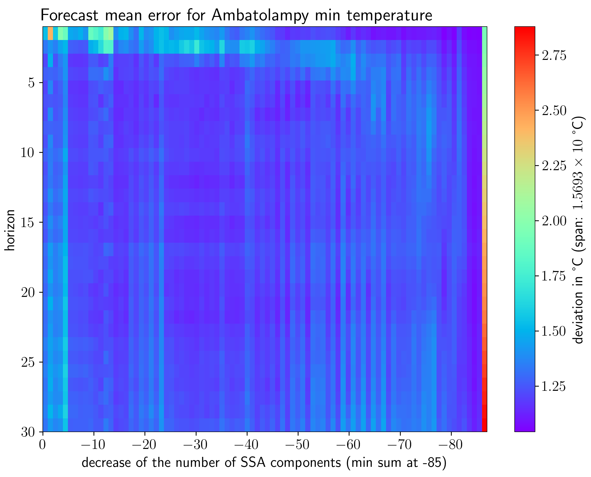
A deeper evaluation relied essentially on the method of [15] with estimating the window length for written . In a more systematic way, for each data set, and every forecasting day, , and have been computed but only and have been used for forecasting with various groupings. More precisely, prefix groupings have been performed for all (resp. ). Fig.1 displays a result of such an exhaustive evaluation. By averaging over the last year of the time series, the best a posteriori prefix grouping (resp. ) with respect to the mean (resp. maximum) forecast error has been selected for comparing with automated groupings computed by grouping.auto.wcor. Also the closest neighbourhood (resp. ) of (resp. ) has been examined. This neighbourhood consists of all index sets that differ from (resp. ) by one element only:
| (5) | ||||
All numerical evaluations were programmed in Python and R. The programs are available upon request from the corresponding author.
8 Results and discussion
As a preamble to this section, it is worth mentioning that the SSA and the corresponding forecasting methods are not considered as learning algorithms. Nevertheless, some analogies with machine learning or their lack are worth highlighting.
-
1.
Undertraining happens exactly as in machine learning when the input time series is too short to capture all essential behaviour of the observed dynamical system. In other words, there is not enough of observations.
-
2.
Overfitting results from the choice of index set including too many inessential components (obtained using SVD). This choice, called “grouping” is discussed in Sect.5. Since those inessential components are considered as noise, a model (an LRE in the case of SSA forecasting) capturing such noise is overfitted.
-
3.
Underfitting is, as usual, the opposite of overfitting. It occurs when index set does not include enough of essential components. The reader should keep in mind that . Thus, when is too small, the underfitting cannot be compensated by a good choice of .
-
4.
The choice of window length does not seem to have a straightforward machine learning counterpart. It can be understood as the choice of the dimension of the model. This is for instance similar to the choice of the number of states of a hidden Markov model (see e.g.[5]) required by spectral learning algorithms [14] or by the classical Baum-Welch algorithm [3, 9]. The choice of can be also compared to the choice of the degree of the polynomial in polynomial regression. Choosing this degree too big leads typically to an overfitting. The potential overfitting when is too big can be however compensated to some extent by the choice of .
While varying day over , computed window lengths , . and remained stable (see Table2). Interestingly, for every considered data set and each , one has
This is surprising as and are the extreme integer values within the real interval which depends only on length of . On the other hand, depends not only on but also on the autocorrelation function (see Eq.4). Consequently, on the contrary to and , depends on the values of . The above inequality is not a general rule and could be attributed to a specific nature of considered data sets, all resulting from atmospheric and oceanic phenomena.
A rough evaluation of forecasting with parameters and confirms the findings of [13, 17, 16] and [20] that using longer windows do not improve forecast accuracy. Indeed, the forecasts obtained within the present experimentation with parameters were not better than random ones. Even with the accuracy was only slightly better than using random forecast. The only convincing results come with and . These are depicted in Appendix B. Their comparison lets conclude that the results obtained with are better than with . Consequently the method of [15] based on the autocorrelation function (see Eq.(4)) is favoured by the authors as it is easy to implement and gives satisfactory results.
A systematic evaluation of prefix grouping for window length shows that the accuracy of forecasting is very sensitive to it. One could think that including more components would better capture the dynamics via an LRE but often the opposite is true. Fig.1 shows how, in prefix grouping, decreasing the number of components affects the forecast. The groupings considered in this example range from down to . One can observe that the mean error does not show any regular pattern. The best accuracy is obtained with when comparing mean errors averaged over all horizons from 1 to 30.
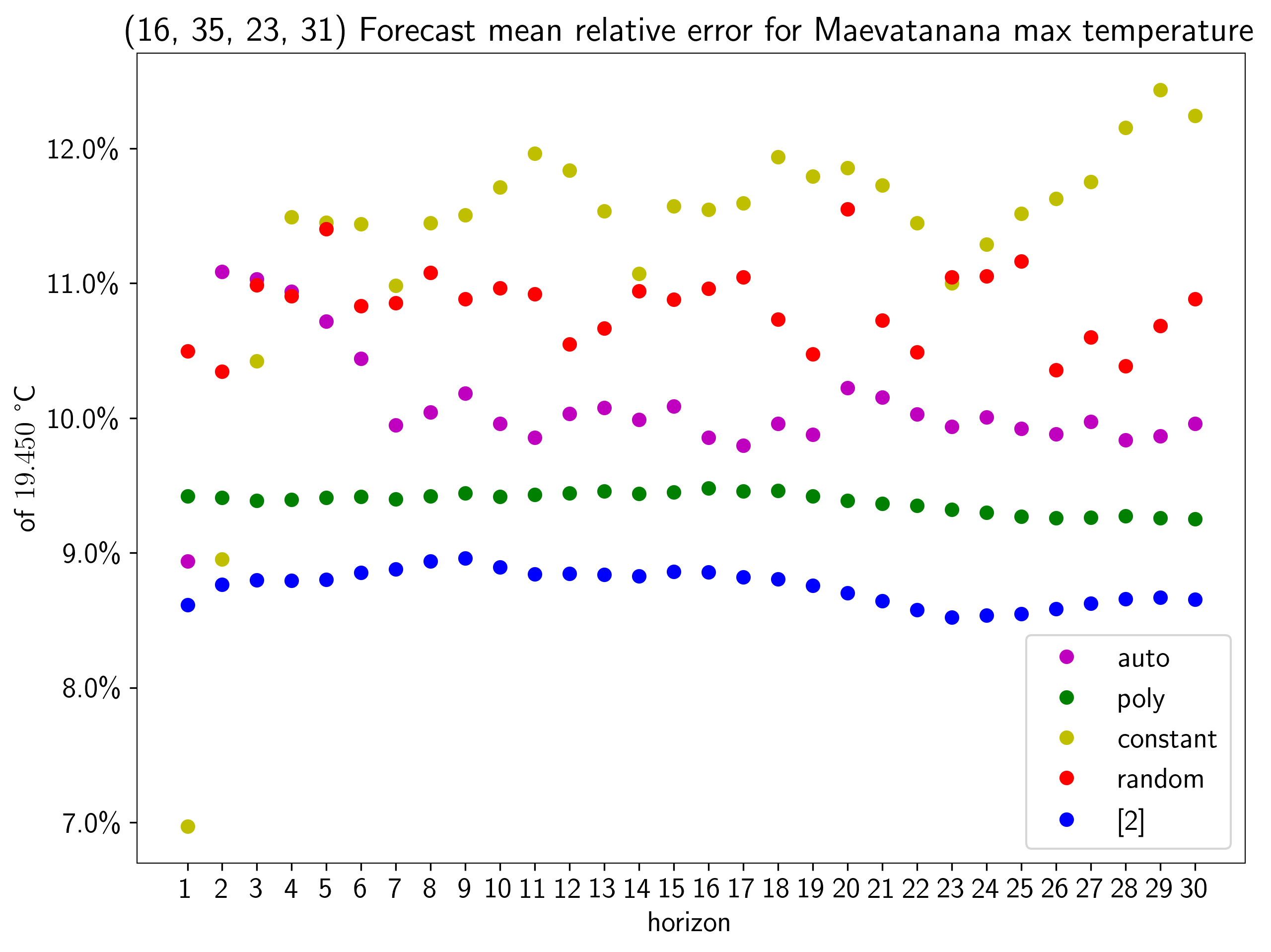
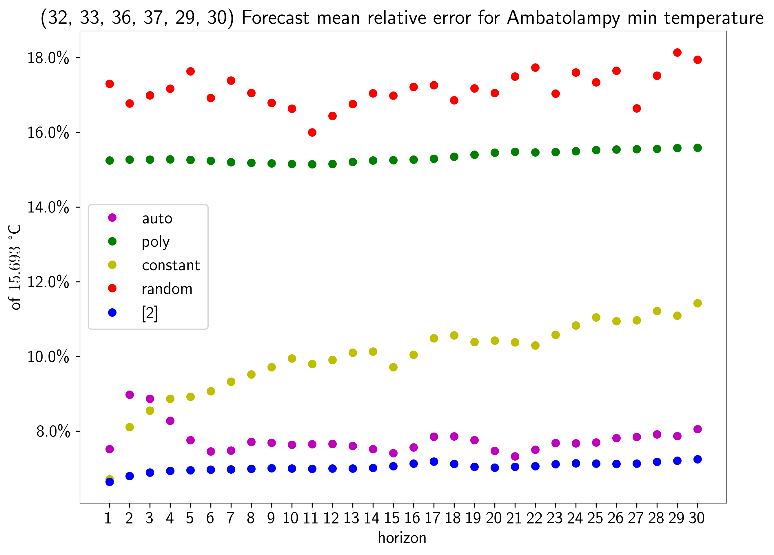
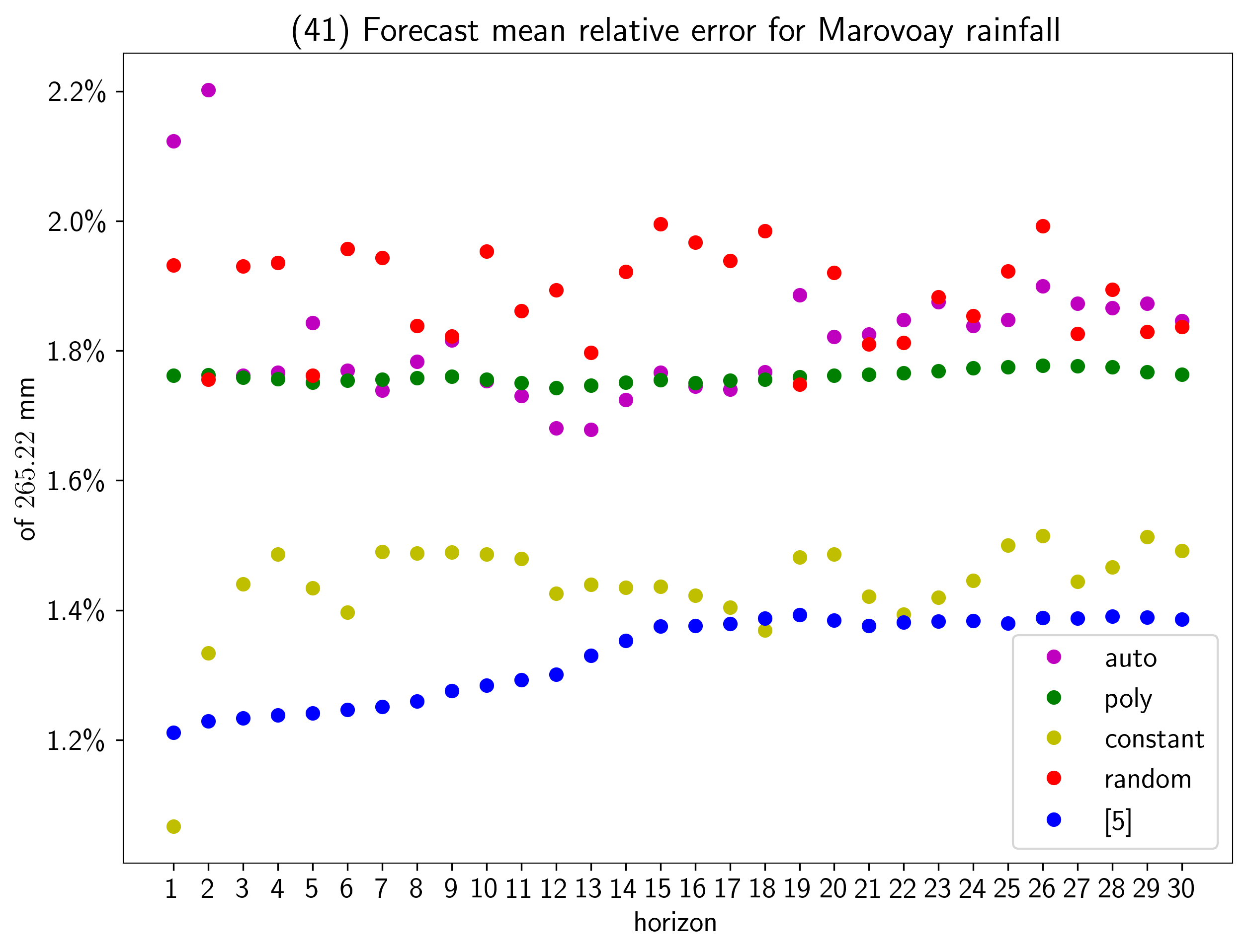
In all time series studied here, the optimal prefix grouping is compared with with clustering-based grouping computed by function grouping.auto.wcor. This is displayed on Fig.2 to 7 which show the mean error per horizon. Similar plots for maximum error appear in Appendix A and use the same colour codes. The errors are plotted in blue for optimum prefix grouping, in purple for the automated grouping, in green for polynomial regression based forecast, in yellow for constant forecast and in red for random forecast. All errors are given relatively to the span of the data set as precised on the left edge of each plot. A surprising observation common to all data sets discussed here is that grouping.auto.wcor always returned a prefix grouping. This is not a general rule. Indeed, for other time series, grouping.auto.wcor may return a cluster of non prefix groupings. Every plot on Fig.2 to 7 has on top the list of groupings, in parentheses, computed by grouping.auto.wcor when varying . More precisely, an integer appearing on the list, means that for some , grouping.auto.wcor returned index set after taking as the input time series. It should be noted here that across , very few different grouping are obtained and that their variation is non-monotonic. As for all plotted forecast errors for horizon , the one resulting from automated grouping is obtained by averaging over . When the mean error is concerned (Fig.2 to 7) the forecasts using automated groupings computed by grouping.auto.wcor clearly appear as sub-optimal. For Marovoay rainfall (Fig.4), that forecast is even close to random forecast and for Maevatanana maximum temperature (Fig.2) a polynomial regression predicts more accurately.
A systematic examination of prefix groupings for confirms the above observations about automated grouping. It also lets comparing forecast accuracy for window lengths and (see figures in Appendix B). As far as mean errors are used for comparison, the automated (resp. optimal) grouping with underperforms the automated (resp. optimal) grouping with in all examples studied, except for Marovoay rainfall. However, when one uses maximum errors (right column) instead of mean errors (left column), no winner can be clearly declared. Moreover, the plots of maximum errors for (see Appendix A) seem to show that the SSA is unsuitable for forecasting when maximum errors are the main concern. Indeed, even with optimal prefix grouping, the maximum error is mostly beyond . This is perhaps a general drawback of all general-purpose forecasting methods for time series, as the maximum error criterion seems to be deliberately avoided in the corresponding literature.
As all groupings discussed in this section are prefix ones, one may ask if, for a given window size, the optimal prefix grouping remains optimal among all groupings. The authors do not know the answer although they observed that the values of the errors in the closest neighbourhoods or (see Eq.(5)) of each optimal prefix groupings (plotted in blue on all figures except on Fig.1) always exceed those of the latter. Therefore, each optimum prefix grouping for data sets considered here form a local minimum. The authors do not know whether this observation could be turned into a theorem nor if such local minima are also global ones. In any case, the latter observation leads to the conclusion that a viable strategy for improving the automated grouping would be to start with the value yield by grouping.auto.wcor and find a nearest local optimum for prefix grouping. The authors believe that similar results to theirs would be obtained from other real world data, as long as they come from systems of intricate dynamics and from sufficiently long time series.
9 Conclusion
The experiments reported in this paper confirm that the choice of the window length and of the grouping are essential for the accuracy of SSA forecasting. The window length selection method of [15] together with an adequate grouping enables forecasting with an accuracy significantly better than constant or random forecasting, provided that the mean error is considered. However, the reader should keep in mind that each adequate (optimal) grouping has been selected via an a posteriori evaluation. The only widely available method for an automated a priori grouping, namely function grouping.auto.wcor from Rssa package, appears as sub-optimal in the analysed examples. Consequently, this is where the research on the SSA should focus in order to make SSA forecasting ready to be included in decision-support tools. In the meantime, the results of this study suggest the following strategy for a practitioner.
-
1.
For every forecasting day, use a fixed-size suffix of the available time series as test data.
-
2.
Perform a local search of a minarg, say , around the set, say , returned by grouping.auto.wcor upon applying SSA forecasting on the training data (viz., the portion of the time series without the test suffix) using test data for evaluating the error, say .
-
3.
Similarly, perform a local search for minarg, say , around prefix grouping . Let be the corresponding evaluation of the error.
-
4.
For today’s forecast, perform SSA steps up to grouping using the whole available time series.
-
5.
If , use group for computing today’s forecast.
-
6.
If , let be the group returned by grouping.auto.wcor. For today’s forecast use group obtained from by translation analogous to that from to .
The results also suggest a preference of the window length selection method of [15] – it outperforms other methods evaluated in reported experiments. If however an implementation of the method of [13] is available, it could be advantageously used, as it simultaneously selects both the window length and the grouping.
When the maximum error matters, SSA forecasting seems rather unsuitable for short horizon prediction, at least for atmospheric/oceanic phenomena illustrated by the time series used in this study. The lack of literature with the maximum error criterion does not let suggest an alternative.
When examining plots of forecasting errors using various methods, one could ask, what could be learned from those about the dynamics of the underlying phenomena. Somewhat intriguing is the fact that the relative position of the plots differs substantially form one time series to another. How to explain that among “naive” forecasting methods the constant one is the worst for Ambatolampy minimum temperature (see Fig3) but the best one for Maevatanana maximum temperature (see Fig2) ?
Acknowledgements
The authors wish to thank Juan Bógalo for general explanation about the circulant SSA and Hong-Guang Ma for clarification about his method for estimating the window length, and both, for providing their Matlab codes.
References
- [1] Carl Eckart and Gale Young “The approximation of one matrix by another of lower rank” In Psychometrika 1, 1936, pp. 211–218
- [2] Roger Penrose “On best approximate solutions of linear matrix equations” In Mathematical Proceedings of the Cambridge Philosophical Society 52.1, 1956, pp. 17–19
- [3] Leonard E. Baum “An Inequality and Associated Maximization Technique in Statistical Estimation of Probabilistic Functions of a Markov Process” In Inequalities 3, 1972, pp. 1–8
- [4] David S. Broomhead and Gregory P. King “Extracting Qualitative Dynamics From Experimental Data” In Physica D: Nonlinear Phenomena 20, 1986, pp. 217–236
- [5] Lawrence R. Rabiner “A tutorial on Hidden Markov Models and selected applications in speech” In Proceedings of the IEEE 77.2, 1989, pp. 257–286
- [6] Robert Vautard and Michael Ghil “Singular Spectrum Analysis in Nonlinear Dynamics with Applications to Paleoclimatic Time Series” In Physica D: Nonlinear Phenomena 35.3, 1989, pp. 395–424
- [7] James R. Elsner and Anastasio A. Tsonis “Singular Spectrum Analysis: a New Tool in Time Series Analysis” Springer, 1996
- [8] Nina Golyandina, Vladimir Nekrutkin and Anatol Zhigljavsky “Analysis of Time Series Structure: SSA and Related Mehtods” ChapmanHall, 2001
- [9] Loyd R. Welch “Hidden Markov models and the Baum-Welch Algorithm” In IEEE Information Theory Society Newsletter 53.4, 2003, pp. 1\bibrangessep10–13 URL: http://www.itsoc.org/publications/nltr/it%5C_dec%5C_03final.pdf
- [10] Myles Allen, Mike Dettinger, Kayo Ide, Dmitri Kondrashov, Michael Ghil, Mike Mann, Andrew W. Robertson, Amira Saunders, Ferenc Varadi, Yudong Tian and Pascal Yiou “The Singular Spectrum Analysis - MultiTaper Method (SSA-MTM) Toolkit”, UCLA Theoretical Climate Dynamics group, 2007 URL: http://research.atmos.ucla.edu/tcd/ssa/
- [11] Peter Grünwald “The minimum description length principle” The MIT Press, 2007
- [12] George Tzagkarakis, Maria Papadopouli and Panagiotis Tsakalides “Trend forecasting based on Singular Spectrum Analysis of traffic workload in a large-scale wireless LAN” In Performance Evaluation 66, 2009, pp. 173–190
- [13] Md Atikur Rahman Khan and Donald S. Poskitt “Description Length Based Signal Detection in Singular Spectrum Analysis”, 2010, pp. 23 pp
- [14] Daniel Hsu, Sham M. Kakade and Tong Zhang “A spectral algorithm for learning Hidden Markov Models” In Journal of Computer and System Sciences 78.5, 2012, pp. 1460–1480
- [15] Hong-Guang Ma, Rong Lei, Xiang-Yu Kong, Zhi-Qiang Liu and Qin-Bo Jiang “Determine a proper window length for singular spectrum analysis” In IET International Conference on Radar Systems (Radar 2012), 2012, pp. 1–6
- [16] Md Atikur Rahman Khan and Donald S. Poskitt “A note on window length selection in singular spectrum analysis” In Australian & New Zealand Journal of Statistics 55.2, 2013, pp. 87–108
- [17] Md Atikur Rahman Khan and Donald S. Poskitt “Moment tests for window length selection in singular spectrum analysis of short– and long–memory processes” In Journal of Time Series Analysis 34.2, 2013, pp. 141–155
- [18] Michael R. Thon and Herbert Jaeger “Links between multiplicity automata, observable operator models and predictive state representations: a unified learning framework” In Journal of Machine Learning Research 16, 2015, pp. 103–147
- [19] Rui Wang, Hong-Guang Ma, Guo-Qing Liu and Dong-Guang Zuo “Selection of window length for singular spectrum analysis” In Journal of the Franklin Institute 352.4, 2015, pp. 1541–1560
- [20] Md Atikur Rahman Khan and Donald S. Poskitt “Forecasting stochastic processes using singular spectrum analysis: Aspects of the theory and application” In International Journal of Forecasting 33.1, 2017, pp. 199–213
- [21] Nina Golyandina, Anton Korobeynikov and Anatol Zhigljavsky “Singular Spectrum Analysis with R” Springer, 2018
- [22] João P. Hespanha “Linear Systems Theory” Princeton University Press, 2018
- [23] Nina Golyandina and Anatol Zhigljavsky “Singular Spectrum Analysis for Time Series” Springer, 2020
- [24] Peter Grünwald and Teemu Roos “Minimum description length revisited” In International Journal of Mathematics for Industry 11.1, 2020, pp. 29 pp
- [25] Hansika Hewamalage, Christoph Bergmeir and Kasun Bandara “Recurrent Neural Networks for Time Series Forecasting: Current status and future directions” In International Journal of Forecasting 37.1, 2021, pp. 388–427
- [26] Anton Korobeynikov, Alex Shlemov, Konstantin Usevich and Nina Golyandina “Rssa: a collection of methods for singular spectrum analysus”, The Comprehensive R Archive Network, 2021 URL: http://CRAN.R-project.org/package=Rssa
- [27] Farnaz Sedighin and Andrzej Cichocki “Image Completion in Embedded Space Using Multistage Tensor Ring Decomposition” In Frontiers in Artificial Intelligence 4, 2021, pp. 11 pp URL: https://doi.org/10.3389/frai.2021.687176
- [28] Rob J Hyndman and George Athanasopoulos “Forecasting: Principles and Practice”, 2023 URL: https://otexts.com/fpp3/
A p p e n d i c e s
Appendix A Maximum error plots for
![[Uncaptioned image]](/html/2403.16507/assets/maeva-mx.png)
![[Uncaptioned image]](/html/2403.16507/assets/ambato-mx.png)
![[Uncaptioned image]](/html/2403.16507/assets/marovo-mx.png)
![[Uncaptioned image]](/html/2403.16507/assets/ambov-mx.png)
![[Uncaptioned image]](/html/2403.16507/assets/analam-mx.png)
![[Uncaptioned image]](/html/2403.16507/assets/comore-mx.png)
Appendix B Comparative plots for two window lengths
The following plots compare the accuracy of vector forecasting for window lengths and . Every label of a legend gives the window size followed by either “auto” for automated grouping using grouping.auto.wcor or the optimal prefix grouping . For (resp. ) the accuracy is plotted in blue (resp. green) for automated grouping and in orange (resp. red) for optimal grouping. The reader may check Table2 to avoid confusion between and . Note that the accuracy obtained with do not appear on the following plots as it is significantly worse than with and .
![[Uncaptioned image]](/html/2403.16507/assets/cmp-maeva-mn.png)
![[Uncaptioned image]](/html/2403.16507/assets/cmp-maeva-mx.png)
![[Uncaptioned image]](/html/2403.16507/assets/cmp-ambato-mn.png)
![[Uncaptioned image]](/html/2403.16507/assets/cmp-ambato-mx.png)
![[Uncaptioned image]](/html/2403.16507/assets/cmp-marovo-mn.png)
![[Uncaptioned image]](/html/2403.16507/assets/cmp-marovo-mx.png)
![[Uncaptioned image]](/html/2403.16507/assets/cmp-ambov-mn.png)
![[Uncaptioned image]](/html/2403.16507/assets/cmp-ambov-mx.png)
![[Uncaptioned image]](/html/2403.16507/assets/cmp-analam-mn.png)
![[Uncaptioned image]](/html/2403.16507/assets/cmp-analam-mx.png)
![[Uncaptioned image]](/html/2403.16507/assets/cmp-comore-mn.png)
![[Uncaptioned image]](/html/2403.16507/assets/cmp-comore-mx.png)