CT-Bound: Fast Boundary Estimation From Noisy Images
Via Hybrid Convolution and Transformer Neural Networks

Abstract

We present CT-Bound, a fast boundary estimation method for noisy images using a hybrid Convolution and Transformer neural network. The proposed architecture decomposes boundary estimation into two tasks: local detection and global regularization of image boundaries. It first estimates a parametric representation of boundary structures only using the input image within a small receptive field and then refines the boundary structure in the parameter domain without accessing the input image. Because of this, a part of the network can be easily trained using naive, synthetic images and still generalized to real images, and the entire architecture is computationally efficient as the boundary refinement is non-iterative and not in the image domain. Compared with the previous highest accuracy methods, our experiment shows that CT-Bound is 100 times faster, producing comparably accurate, high-quality boundary and color maps. We also demonstrate that CT-Bound can produce boundary and color maps on real captured images without extra fine-tuning and real-time boundary map and color map videos at ten frames per second.

Index Terms—  Boundary estimation, image denoising, convolutional neural network, transformer

1 Introduction

Estimating boundary structures from images is a foundational computer vision problem that has broad downstream applications in medical imaging, manufacturing, autonomous navigation, etc. This problem can become extremely challenging when the input images are noisy due to common reasons, such as insufficient photons received on the cameras’ photon detectors during the exposure. Although image boundary estimation has been broadly studied since the early stage of computer vision decades ago [4, 5, 6], current solutions either produce low-quality boundary maps or require an infeasible processing time for real-time applications to search for a satisfactory result when the images are noisy (Fig. LABEL:fig:teaser).

We present CT-Bound. It is a fast, deep neural network that performs image boundary estimation on noisy images. The architecture outputs a generalized image boundary parameterization, namely the Field of Junctions (FoJs) [1]. The FoJ is a data structure that can model a variety of boundary types in image patches, including edges, corners, and contours, using a few parameters. Compared to the non-data-driven, iterative solver presented in the original FoJ paper that estimates the FoJ of a $147\times 147$ resolution image using 60 secs, the proposed approach is complementary as it is data-driven and non-iterative and is 100 times faster while maintaining similar accuracy and visual quality (Fig. LABEL:fig:teaser).

CT-Bound consists of an innovative two-stage, hybrid Convolution and Transformer neural network architecture (Fig. 2). The first stage is a convolutional architecture that makes an initial prediction of a local FoJ parameterization solely based on the visual appearance of each image patch. The second stage consists of a feedforward transformer encoder that takes in the initial FoJ estimation of all image patches to perform refinement. The architecture is novel as it completely decomposes boundary estimation into two computer vision tasks: detecting boundaries from local image appearance and regularizing neighboring boundary estimations to ensure consistency and to look like natural boundaries. The convolutional network stage conducts boundary detection using a small receptive field ($21\times 21$ in our experiments). Thus, it does not need to learn the global appearance of images and can be trained using synthetic image patches that only contain basic boundary structures. The transformer stage only receives the FoJ representation and has no access to the input image during inference. Therefore, the computational complexity of the transformer in the CT-Bound is significantly lower than that of the classic Vision Transformer [7].

We verify the accuracy and robustness of CT-Bound using noisy images simulated from standard, benchmark datasets under different noise levels. We also validate the accuracy of the proposed algorithm using real-world noisy images captured using our experimental setup. To conclude, the contribution of this paper includes:

• An invention of a two-stage, hybrid neural network architecture;

• A fast and non-iterative solver of field-of-junctions that enables real-time accurate boundary estimation on noisy images;

• A thorough experimental study of the proposed architecture using synthetic and real data.

The code, the training data, the testing data, and the video demonstration of the proposed method can be found at https://github.com/guo-research-group/CT-Bound.

2 Related Work

According to the classification by Gong et al. [8], boundary detection from images can be divided into four categories, i.e., boundaries from luminance changes, texture changes, perceptual grouping, and illusory contour. We focus our literature review on the first category to which the proposed method belongs.

Local boundary detection.

The first step of boundary detection is typically using specially designed filters to locate local responses of image boundaries. The filters either maximize the detectability and localization accuracy of the boundaries under noise, such as the Canny detectors [4], the Laplacian detectors [9], and the perfect matching filters [10] or are sensitive to the direction of the image boundaries, e.g., Sobel filters [5], Gaussian quadrature pairs [6], Steerable filters [11], etc. To robustly detect boundaries under non-ideal edges, people also develop sophisticated filters that are non-linear [12] or operate in multiple scales [13]. However, these classic methods based on local patches are found to be insufficient when the noise of the image is severe and have limited visual information to confidently determine the edges from the receptive field of a single filter. In this case, image smoothing is also not a solution as the smoothing operation will make faint or fine boundary structures to be indistinguishable [10].

Global boundary refinement.

Boundaries in natural images are usually piece-wise smooth. Based on this observation, people have developed algorithms to refine the global boundary map from the locally detected boundaries by regularizing the curvature, for example, the squared curvature [14] or total curvature [15] along the boundary. Another observation for global boundary refinement is that the neighboring boundary maps must agree. There have been methods that use this intuition by enforcing neighboring consistency [1, 16]. These global refinement methods are typically iterative and thus could have a high computational complexity.

Deep learning boundary detection.

The emergence of deep learning has enabled people to develop deep neural networks to directly output global boundary maps in a nonparametric way [17, 18] or a parametric way [19, 20], segmentation maps [21], etc. The proposed method is complementary to the current literature as it performs fast, parametric boundary estimation specifically for images at low SNR.

3 Methods

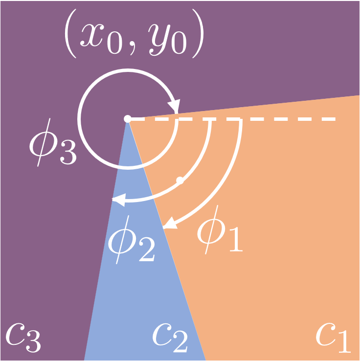
Fig. 1: Field-of-junction (FoJ) representation [1].

We first briefly describe the FoJ representation [1] that we adopt in this work. Given an image patch $P\in\mathbb{R}^{h\times w\times k}$ with dimension $h\times w$ and $k$ color channel, the FoJ models its boundary structure using a parameter set $\Phi=(\boldsymbol{x},\boldsymbol{\phi},\boldsymbol{c})$, where $\boldsymbol{x}=(x_{0},y_{0})$ indicates the center of the vertex, $\boldsymbol{\phi}=(\phi_{1},\cdots,\phi_{l})$ represents the angles of the $l$ edges, $\boldsymbol{c}=(\boldsymbol{c}_{1},\cdots,\boldsymbol{c}_{l}),\boldsymbol{c}_{j}\in\mathbb{R}^{k},j=1,\cdots,l$ are the color of the region between every pair of neighboring edges. The parameter $l$ is a hyperparameter that needs to be predetermined. See Fig. 1 for an exemplar illustration of FoJ with $l=3$. As shown in Verbin and Zickler, FoJ can represent a variety of local boundary structures, including edges, corners, and junctions [1]. Given an FoJ representation $\Phi$, the corresponding boundary map of the patch $B(x,y;\Phi)$ can be plotted via:

$$B(x,y;\Phi)=\pi\epsilon H_{2,\epsilon}^{\prime}(\min(d_{j}(x,y))),$$ (1)

where $d_{j}(x,y)$ is the distance from the pixel $(x,y)$ to the edge $j$ and $H_{2,\epsilon}^{\prime}$ is the derivative of Heaviside function $H_{2,\epsilon}$ defined in [22]:

$$H_{2,\epsilon}(d)=\frac{1}{2}\left(1+\frac{2}{\pi}\arctan\frac{d}{\epsilon}\right),$$ (2)

where $\epsilon$ is a smoothing parameter that we set $\epsilon=0.01$ throughout our experiments. The color map $C(x,y;\Phi)$ can be visualized using:

$$C(x,y;\Phi)=\sum_{j=1}^{l}\delta_{j}(x,y)\boldsymbol{c}_{j},$$ (3)

where $\delta_{j}(x,y)=1$ when the pixel $(x,y)$ is within the wedge between edge $j$ and $j+1$ in the patch $P$:

$$\Omega_{j}=\{ (x,y)|(x,y)\in P,$$ (4)

$$(x-x_{0})\cos\phi_{j}+(y-y_{0})\sin\phi_{j}<0,$$

$$(x-x_{0})\cos\phi_{j+1}+(y-y_{0})\sin\phi_{j+1}>0\},$$

and $\delta_{j}(x,y)=0$ otherwise.

Specifically, we use $l=3$ in our implementation.

3.1 Network architecture

The network architecture of the proposed method is visualized in Fig. 2. Given a noisy image $I\in\mathbb{R}^{H\times W\times k}$, CT-Bound first divides the image $I$ into overlapping patches. The initialization stage takes in each image patch $P_{m,n}$ into a CNN to generate the initial vertex location and the edge angles of the FoJ representation $(\boldsymbol{x}^{\text{init}}_{m,n},\boldsymbol{\phi}^{\text{init}}_{m,n})$. Then, the method determines the color parameters $\boldsymbol{c}^{\text{init}}_{m,n}=(\boldsymbol{c}^{\text{init}}_{m,n,1},\cdots,\boldsymbol{c}^{\text{init}}_{m,n,l})$ mathematically by averaging the color of pixels of each divided area of the patch:

$$\boldsymbol{c}^{\text{init}}_{m,n,j}=\frac{1}{|\Omega_{m,n,j}|}\sum_{(x,y)\in\Omega_{m,n,j}}P_{m,n}(x,y,:),$$ (5)

where $\Omega_{m,n,j}$ indicates the set of pixels in the wedge between edges $j$ and $j+1$ in the patch $P_{m,n}$, as defined in Eq. 4.

The refinement stage takes in the initial FoJ representation $(\boldsymbol{x}^{\text{init}}_{m,n},$ $\boldsymbol{\phi}^{\text{init}}_{m,n},$ $\boldsymbol{c}^{\text{init}}_{m,n})$ of all patches $P_{m,n}$ simultaneously. It first converts each initial FoJ representation $(\boldsymbol{x}^{\text{init}}_{m,n},\boldsymbol{\phi}^{\text{init}}_{m,n},$ $\boldsymbol{c}^{\text{init}}_{m,n})$ into a feature vector representation $\boldsymbol{v}_{m,n}\in\mathbb{R}^{d}$, and applies positional encoding by adding a positional vector $\boldsymbol{p}_{m,n}=[p_{m,n,1},\cdots,p_{m,n,d}]^{T}$ to the feature vector $\boldsymbol{v}_{m,n}$ to incorporate the positional information of each image patch. The 2D positional encoding vector follows the design of Wang and Liu [23]:

$$p_{m,n,i} =\begin{cases}\sin\left(\frac{m}{10000^{4i/D}}\right),i=0,2,4,\cdots,d/2\\ \cos\left(\frac{m}{10000^{4i/D}}\right),i=1,3,5,\cdots,d/2+1\\ \sin\left(\frac{n}{10000^{4i/D}}\right),i=d/2,d/2+2,\cdots,d-2\\ \cos\left(\frac{n}{10000^{4i/D}}\right),i=d/2+1,d/2+3,\cdots,d-1\end{cases}$$

where the dimension of each feature vector $d$ is an even number. All positional encoded feature vectors are fed into a transformer encoder consisting of a series of multi-head attention layers to refine the boundary consistency among patches globally and adjust unnatural boundary estimations. It is the only block in the framework that globally shares the per-patch FoJ information. Finally, the framework outputs the refined vertex location and edge angles of all patches $(\boldsymbol{x}^{\text{ref}}_{m,n},\boldsymbol{\phi}^{\text{ref}}_{m,n}),\forall m,n$, and calculate the refined color parameters $\boldsymbol{c}^{\text{ref}}_{m,n}$ using Eq. 5. We list the network hyperparameters we use in our experiment in Tab. 1. As the transformer does not operate on the image domain, the dimension of the input vector and the number of layers are much smaller compared to the classic Vision Transformer [7].

From the refined FoJ parameters $\Phi^{\text{ref}}_{m,n}=(\boldsymbol{x}^{\text{ref}}_{m,n},$ $\boldsymbol{\phi}^{\text{ref}}_{m,n},$ $\boldsymbol{c}^{\text{ref}}_{m,n})$, CT-Bound generates the per-patch boundary and color map according to Eq. 1 and 3, and computes the global boundary map $B(x,y)$ by averaging the per-patch boundary maps [1]:

$$B(x,y)=\frac{1}{N(x,y)}\sum_{N(x,y)}B(x,y;\Phi^{\text{ref}}_{m,n})$$ (6)

and the global color map $C(x,y)$ via a specific smoothing operation over the per-patch color maps:

$$C(x,y)=\frac{1}{\left|N(x,y)\right|}\sum_{N(x,y)}\delta_{m,n,j}(x,y)\boldsymbol{c}^{\text{ref}}_{m,n,j}$$ (7)

where $N(x,y)=\left\{(m,n)|(x,y)\in\Omega_{m,n,j}\right\}$ is the set of the patch indices that contain $(x,y)$, $\delta_{m,n,j}$ is a binary indicator that is $1$ if pixel $(x,y)$ belongs to the wedge $\Omega_{m,n,j}$ and $0$ otherwise, and $\boldsymbol{c}^{\text{ref}}_{m,n,j}$ is the refined color of wedge $\Omega_{m,n,j}$.

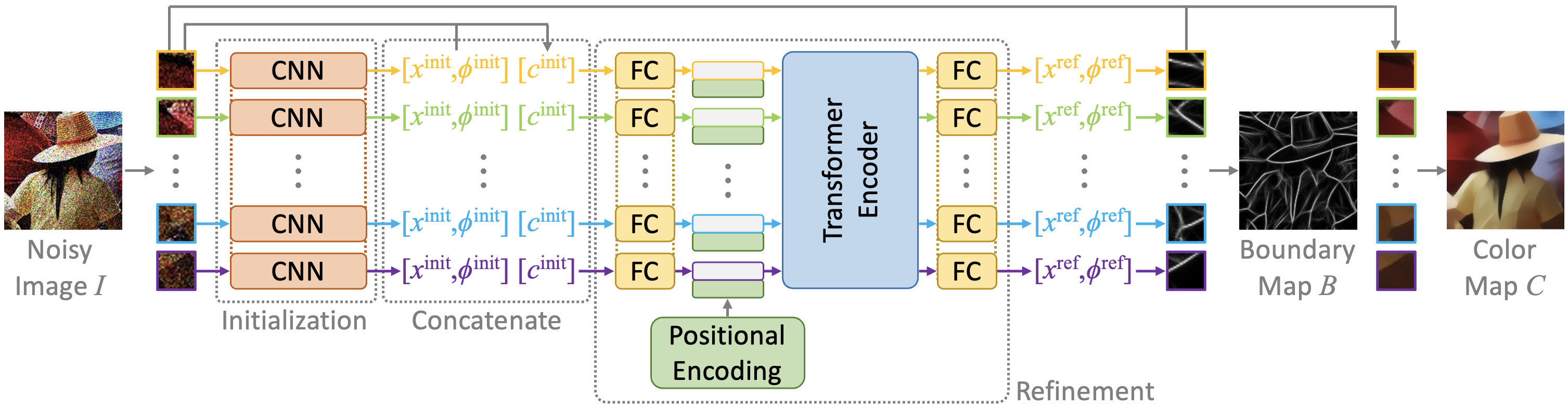
Fig. 2: Network architecture of CT-Bound. The architecture consists of two stages. The initialization stage contains shared-weights convolutional neural networks that output the FoJ representation of every image patch. The refinement stage consists of a transformer encoder that simultaneously refines all per-patch FoJ representations. Finally, the framework combines all per-patch FoJ representations together to output the global boundary map and the color map.

3.2 Loss functions

We develop a multi-stage training scheme to optimize the parameters of CT-Bound. First, we train the initialization stage using the patch reconstruction loss:

$$\mathcal{L}_{\text{init}}=\mathbb{E}_{P}\left(\mathrm{MSE}\left(C\left(x,y;\Phi^{\text{gt}}\right),C\left(x,y;\Phi^{\text{init}}\right)\right)\right),$$ (8)

where $\mathbb{E}_{P}$ denotes the expectation over all patches in the training set, and $C(x,y;$ $\Phi^{\text{gt}})$ and $C(x,y;\Phi^{\text{init}})$ indicate the per-patch color maps reconstructed using true and estimated FoJ parameters, respectively. We observe that the visual quality of the FoJ estimation is higher when using the loss in Eq. 8 for training than directly supervising the FoJ parameters. Furthermore, because the CNN in the initialization stage has a small receptive field, we can use synthetic image patches of basic shapes to train it, and we observe that the trained model can be generalized to real-world image patches without further finetuning.

When optimizing parameters of the refinement stage, we use a fixed, pre-trained initialization stage to generate inputs $\Phi^{\text{init}}$. We invent a two-step training process for optimizing the refinement stage, which was noticed to lead to a more stable and faster convergence. In the first step, a mean squared error loss function is adopted to supervise the estimated FoJ parameters directly:

$$\mathcal{L}_{\text{ref1}}=\mathbb{E}_{P}\left(\lVert\boldsymbol{x}^{gt}-\boldsymbol{x}^{\text{ref}}\rVert^{2}+\lVert\boldsymbol{\phi}^{gt}-\boldsymbol{\phi}^{\text{ref}}\rVert^{2}\right).$$ (9)

In the second step, we use a comprehensive image reconstruction loss adapted from Verbin and Zickler [1]:

$$\mathcal{L}_{\text{ref2}}=\mathbb{E}_{I}\left(l_{p}+\lambda_{b}l_{b}+\lambda_{c}l_{c}\right),$$ (10)

where $\mathbb{E}_{I}$ indicates the expectation over all images in the dataset, and $l_{p}$, $l_{b}$, and $l_{c}$ are patch, boundary, and color loss terms, respectively:

$$l_{p} =\sum_{m,n}\sum_{j=1}^{l}\sum_{x,y}\delta_{m,n,j}(x,y)\lVert\boldsymbol{c}^{\text{ref}}_{m,n,j}-I(x,y)\rVert^{2},$$

$$l_{b} =\sum_{m,n}\sum_{x,y}\left(B(x,y)-B(x,y;\Phi^{\text{ref}}_{m,n})\right)^{2},$$

$$l_{c} =\sum_{m,n}\sum_{j=1}^{l}\sum_{x,y}\delta_{m,n,j}(x,y)\lVert\boldsymbol{c}^{\text{ref}}_{m,n,j}-C(x,y)\rVert^{2}.$$

In Verbin and Zickler, the loss in Eq. 10 was solved in an alternating, two-step fashion to refine the FoJ representation iteratively [1]. We evaluate the loss in a single step and show it can successfully fine-tune the feed-forward transformer encoder to improve the FoJ representation.

Table 1: CT-Bound model hyperparameter.

Convolutional Neural Network
Layer	Specification	Output
Conv2d	5$\times$5 kernel, 4 stride, 2 pad	(21, 21, 96)
MaxPool2d	3$\times$3 kernel, 2 stride, 0 pad	(10, 10, 96)
Conv2d	5$\times$5 kernel, 1 stride, 2 pad	(10, 10, 256)
MaxPool2d	2$\times$2 kernel, 2 stride, 0 pad	(5, 5, 256)
Conv2d	3$\times$3 kernel, 1 stride, 1 pad	(5, 5, 384)
Conv2d	3$\times$3 kernel, 1 stride, 1 pad	(5, 5, 384)
Conv2d	3$\times$3 kernel, 1 stride, 1 pad	(5, 5, 256)
MaxPool2d	3$\times$3 kernel, 2 stride, 0 pad	(2, 2, 256)
FC	-	4096
FC	-	1024
FC	-	5

Transformer Encoder
Specification	Parameter
Dimension of each input vector	128
Number of layers	8
Number of heads in each layer	8
Dimension of the feed-forward layer	256

3.3 Boundary selection and edge localization error

We use the color difference between both sides of an edge as a metric to quantify the detectability of each edge and analyze the edge localization accuracy under different detectability thresholds. In our experiment, we compute the relative color difference $\Delta C_{m,n,j}$ of edge $j$ in patch $P_{m,n}$ as the normalized distance of the color parameters on both sides of an edge in the sRGB space:

$$\Delta C_{m,n,j}=\lVert\boldsymbol{c}^{\text{ref}}_{m,n,j}-\boldsymbol{c}^{\text{ref}}_{m,n,j+1}\rVert/\alpha,$$ (11)

where $\alpha$ is the photon level of the image. More description of $\alpha$ is in Sec. 4.1. We remove the predicted edges from the global boundary in the FoJ representation if the relative color difference is below a specific threshold $\Delta C_{\text{thre}}$. The same process is repeated on the ground truth FoJ representation. To calculate the edge localization error, we binarize the predicted global boundary map $B(x,y)$ and the ground truth boundary map $B^{gt}(x,y)$ and calculate the average distance of each predicted boundary pixel to the nearest ground truth boundary pixel. We report the edge localization error under several thresholds $\Delta C_{\text{thre}}$ in Sec. 4.

4 Experimental Results

4.1 Data processing

For the training of the initialization stage, we use randomly sampled patches from FoJ synthetic datasets [1] that only contain images of basic shapes such as squares. We select $8000$ image patches for training and $2000$ for testing. To simulate image noise, we apply a Poisson process to each image patch [24]:

$$P(x,y)=\text{Poisson}(\alpha P^{*}(x,y)),$$ (12)

where $P(x,y)$ and $P^{*}(x,y)\in[0,1]$ are the noisy and normalized clean image patches, and $\alpha$ is the photon level parameter that controls the noise of the image. For the refinement stage, we use images from MS COCO [25] for training and testing. The training and testing sets contain $1600$ and $400$ randomly selected, non-overlapping images, respectively. Each image is cropped at the center to have the uniform shape $147\times 147$ and is applied with the same noise as described in Eq. 12. In our experiment, we randomly set the photon level $\alpha$ within the range $[2,10]$ to generate images with a variety of noise levels.

4.2 Training specification and network architecture

All optimization in this work uses Adam optimizer [26]. The initialization stage is trained with an initial learning rate of $0.0002$ and a decay of $0.5$ every $80$ epochs. The total number of training epochs is $900$, and the batch size is $32$. We use a two-step scheme to train the refinement stage as described in Sec. 3.2. The first step uses Eq. 9 as the objective function and has $100$ epochs. a learning rate $5\times 10^{-5}$. The second step switches to Eq. 10 as its loss function and runs $1600$ epochs. The learning rate for the second step is updated with a triangular cycle between $1.75\times 10^{-4}$ and $3.5\times 10^{-4}$. Both steps use a batch size $16$. The training and testing of this work is performed on a machine with NVIDIA GeForce RTX A5000 graphics card and 24 GB memory.

4.3 Ablation study

We analyze the benefit offered by the refinement stage of CT-Bound. As shown in Fig. 3a-f, the refinement stage attenuates noisy and inconsistent boundary estimations and strengthens real boundaries compared to the boundary map from the initialization stage. It also makes the color map appear smoother and sharper at color boundaries. The quantitative analysis in Tab. 2 draws the same conclusion: the refinement stage reduces the edge localization error of the boundary map by at least three times compared to that from the initialization stage.

Fig. 3f-h visualizes how the boundary selection mechanism can filter out faint edges with a low color difference. Fig. 3f-h shows filtered boundary maps with relative color difference threshold $\Delta C_{\text{thre}}=0,0.1,0.2$, respectively. We report the mean edge localization error of boundary maps filtered under these three thresholds in all subsequent analyses.

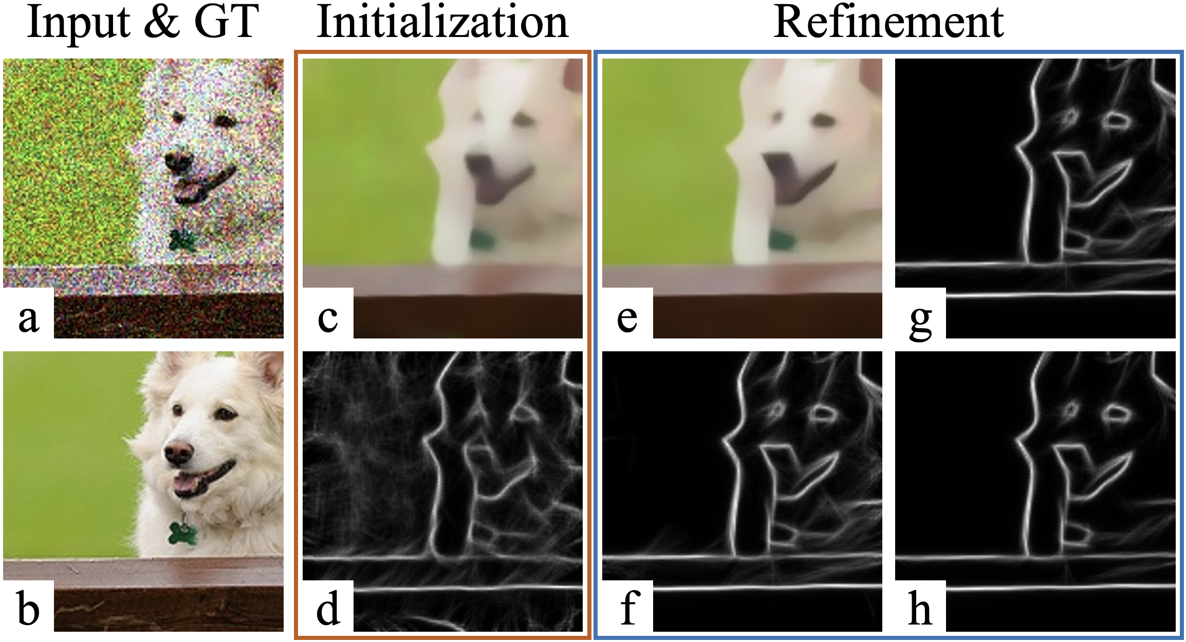
Fig. 3: Effect of refinement and boundary selection. (a-b) An input noisy image and the corresponding clean image from the MS COCO dataset [25]. (c-d) The color map and boundary map before the refinement stage. (e-f) The color map and boundary map after the refinement stage. Noisy edge estimations are removed in refinement, and the color map is smoother. (g) Selected boundaries with $\Delta C_{\text{thre}}=0.1$. (h) Selected boundaries with $\Delta C_{\text{thre}}=0.2$. Estimated boundaries corresponding to low color differences are filtered out.

Table 2: Accuracy of CT-Bound before (numbers in red) and after (numbers in blue) the refinement. Both initialization and refinement stages are trained using images with random photon level $\alpha\in[2,10]$ and are tested under images with specific photon levels. The metric $D(\Delta C_{\text{thre}})$ is the mean edge localization error (unit in pixel) for edges with a relative color difference higher than the threshold $\Delta C_{\text{thre}}$. The refinement significantly reduce the error of boundary estimation.

Photon level	Boundary map			Color map
	$D(0)$$\downarrow$	$D(0.1)$$\downarrow$	$D(0.2)$$\downarrow$	SSIM$\uparrow$	PSNR(dB)$\uparrow$	MSE$\downarrow$
2	1.5138	4.7354	6.2434	0.8787	37.4253	0.0662
	0.3692	0.4049	0.4577	0.9085	39.2779	0.0426
6	1.3845	3.0183	3.3110	0.6675	28.0287	0.5841
	0.3974	0.4701	0.6156	0.7570	30.8394	0.3181
10	1.3769	2.4024	2.8537	0.5470	23.6156	1.6189
	0.4362	0.5511	0.5043	0.6622	26.5821	0.8678

4.4 Analysis on synthetic and real images

We compare the proposed method with the iterative FoJ solver [1], the highest-performing boundary estimation method under low signal-to-noise ratios to our knowledge. As a reference, we also compare with other deep learning-based approaches, including DnCNN [2] + Canny detector [4], and directly predicting the boundary and color maps from a U-Net [3]. Tab. 3 shows the quantitative comparison of these methods. The proposed approach achieves the highest accuracy in boundary estimation and the best quality in color map estimation under all metrics. Meanwhile, it is more than 100 times faster than the iterative FoJ solver. Fig. 4 shows sample boundary maps and color maps estimated from noisy images synthesized from the MS-COCO dataset. The boundary maps of the proposed method are visually clean, and the color maps are smooth with sharp boundaries.

Table 3: Quantitative comparison on noisy images synthesized from MS-COCO dataset [25]. The first column indicates the testing images’ photon level $\alpha_{\text{test}}$ and shows a sample image. FoJ init. and FoJ ref. represents using the first stage only and using the entire framework of the iterative FoJ solver [1], respectively. DnCNN, U-Net, and Ours are trained using images with random photon level $\alpha_{\text{train}}\in[2,10]$ and tested on a specific photon level $\alpha_{\text{test}}$. The metric $D(\Delta C_{\text{thre}})$ is the mean edge localization error (unit in pixel) for edges with a relative color difference higher than the threshold $\Delta C_{\text{thre}}$. Boundary maps generated by DnCNN with the help of Canny and U-Net (a threshold $45/255$ is used the binarize the boundary map channel) are both binary, so only $D(0)$ is applied. Our method achieves the highest performance on both $\alpha=2$ and $10$, indicating the robustness of the proposed method to the image noise level.

Photon level $\alpha_{\text{test}}$		Model	Boundary map			Color map			Running time (s)$\downarrow$
			$D(0)$$\downarrow$	$D(0.1)$$\downarrow$	$D(0.2)$$\downarrow$	SSIM$\uparrow$	PSNR (dB)$\uparrow$	MSE$\downarrow$
2		FoJ init. [1]	0.8796	0.8257	0.5383	0.8110	35.8816	0.3081	20.3268
		FoJ ref. [1]	0.7946	1.0802	0.6317	0.8173	36.0555	0.3066	67.9027
		DnCNN [2](+Canny [4])	1.6841	-	-	0.5150	9.8142	0.4567	0.0092
		U-Net [3]	1.6425	-	-	0.5959	31.1730	0.2585	0.0532
		Ours	0.3692	0.4049	0.4577	0.9085	39.2779	0.0426	0.0875
10		FoJ init. [1]	0.5975	2.9391	1.0558	0.5808	25.9343	1.0927	-
		FoJ ref. [1]	0.5497	3.4584	1.5912	0.6044	26.4057	0.9953	same
		DnCNN [2](+Canny [4])	2.1304	-	-	0.4462	12.7419	1.7578	as
		U-Net [3]	1.3641	-	-	0.4021	20.1722	3.2727	above
		Ours	0.4362	0.5511	0.5043	0.6622	26.5821	0.8678	-

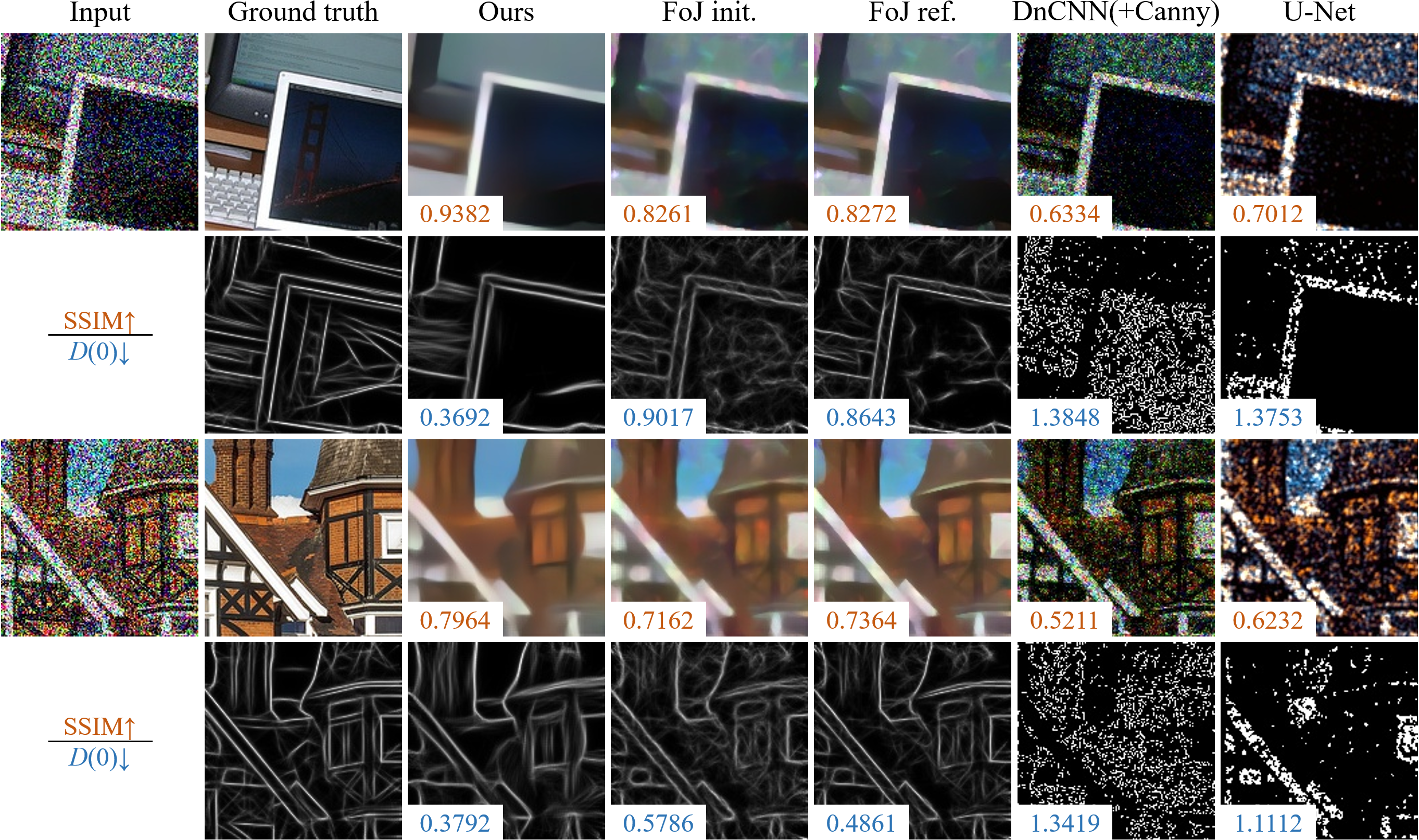
Fig. 4: Qualitative comparison of noisy images synthesized from MS-COCO dataset [25]. Photon level $\alpha=2$.

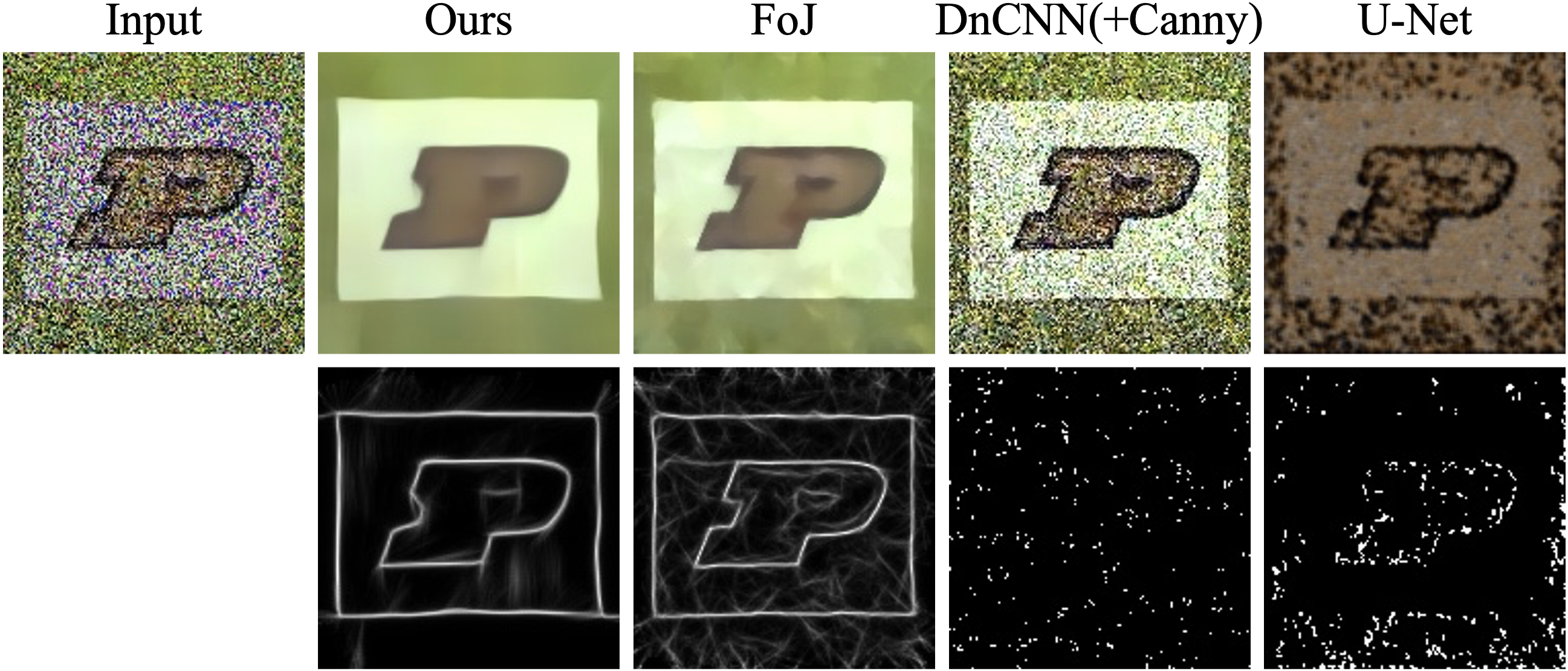
Fig. 5: Comparison using real captured images. The image is taken at the exposure of 1/10900s and ISO 40.

Fig. 5 shows the boundary maps and color maps estimated from a real image captured by an iPhone 13 Mini camera with a high shutter speed. The boundary map and color map generated from the proposed method have high visual quality without any fine-tuning to the real images. We also upload a video of boundary maps and color maps of a real captured video clip generated by the proposed method in the URL listed in the introduction.

References

- [1] Dor Verbin and Todd Zickler, “Field of junctions: Extracting boundary structure at low snr,” in Proceedings of the IEEE/CVF International Conference on Computer Vision, 2021, pp. 6869–6878.
- [2] Kai Zhang, Wangmeng Zuo, Yunjin Chen, Deyu Meng, and Lei Zhang, “Beyond a gaussian denoiser: Residual learning of deep cnn for image denoising,” IEEE transactions on image processing, vol. 26, no. 7, pp. 3142–3155, 2017.
- [3] Olaf Ronneberger, Philipp Fischer, and Thomas Brox, “U-net: Convolutional networks for biomedical image segmentation,” in Medical Image Computing and Computer-Assisted Intervention–MICCAI 2015: 18th International Conference, Munich, Germany, October 5-9, 2015, Proceedings, Part III 18. Springer, 2015, pp. 234–241.
- [4] John Canny, “A computational approach to edge detection,” IEEE Transactions on pattern analysis and machine intelligence, , no. 6, pp. 679–698, 1986.
- [5] FG Irwin et al., “An isotropic 3x3 image gradient operator,” Presentation at Stanford AI Project, vol. 1968, pp. 3, 2014.
- [6] Jitendra Malik, Serge Belongie, Thomas Leung, and Jianbo Shi, “Contour and texture analysis for image segmentation,” International journal of computer vision, vol. 43, pp. 7–27, 2001.
- [7] Alexey Dosovitskiy, Lucas Beyer, Alexander Kolesnikov, Dirk Weissenborn, Xiaohua Zhai, Thomas Unterthiner, Mostafa Dehghani, Matthias Minderer, Georg Heigold, Sylvain Gelly, et al., “An image is worth 16x16 words: Transformers for image recognition at scale,” arXiv preprint arXiv:2010.11929, 2020.
- [8] Xin-Yi Gong, Hu Su, De Xu, Zheng-Tao Zhang, Fei Shen, and Hua-Bin Yang, “An overview of contour detection approaches,” International Journal of Automation and Computing, vol. 15, pp. 656–672, 2018.
- [9] Xin Wang, “Laplacian operator-based edge detectors,” IEEE transactions on pattern analysis and machine intelligence, vol. 29, no. 5, pp. 886–890, 2007.
- [10] Nati Ofir, Meirav Galun, Sharon Alpert, Achi Brandt, Boaz Nadler, and Ronen Basri, “On detection of faint edges in noisy images,” IEEE transactions on pattern analysis and machine intelligence, vol. 42, no. 4, pp. 894–908, 2019.
- [11] William T Freeman, Edward H Adelson, et al., “The design and use of steerable filters,” IEEE Transactions on Pattern analysis and machine intelligence, vol. 13, no. 9, pp. 891–906, 1991.
- [12] Pietro Perona, Jitendra Malik, et al., “Detecting and localizing edges composed of steps, peaks and roofs,” 1991.
- [13] Y. Lu and R.C. Jain, “Reasoning about edges in scale space,” IEEE Transactions on Pattern Analysis and Machine Intelligence, vol. 14, no. 4, pp. 450–468, 1992.
- [14] Claudia Nieuwenhuis, Eno Toeppe, Lena Gorelick, Olga Veksler, and Yuri Boykov, “Efficient squared curvature,” in Proceedings of the IEEE Conference on Computer Vision and Pattern Recognition, 2014, pp. 4098–4105.
- [15] Qiuxiang Zhong, Yutong Li, Yijie Yang, and Yuping Duan, “Minimizing discrete total curvature for image processing,” in Proceedings of the IEEE/CVF Conference on Computer Vision and Pattern Recognition, 2020, pp. 9474–9482.
- [16] Nati Ofir, Meirav Galun, Boaz Nadler, and Ronen Basri, “Fast detection of curved edges at low snr,” in Proceedings of the IEEE Conference on Computer Vision and Pattern Recognition, 2016, pp. 213–221.
- [17] Saining Xie and Zhuowen Tu, “Holistically-nested edge detection,” in Proceedings of the IEEE international conference on computer vision, 2015, pp. 1395–1403.
- [18] Xavier Soria Poma, Edgar Riba, and Angel Sappa, “Dense extreme inception network: Towards a robust cnn model for edge detection,” in Proceedings of the IEEE/CVF winter conference on applications of computer vision, 2020, pp. 1923–1932.
- [19] Kun Huang, Yifan Wang, Zihan Zhou, Tianjiao Ding, Shenghua Gao, and Yi Ma, “Learning to parse wireframes in images of man-made environments,” in Proceedings of the IEEE Conference on Computer Vision and Pattern Recognition, 2018, pp. 626–635.
- [20] Nan Xue, Song Bai, Fudong Wang, Gui-Song Xia, Tianfu Wu, and Liangpei Zhang, “Learning attraction field representation for robust line segment detection,” in Proceedings of the IEEE/CVF Conference on Computer Vision and Pattern Recognition, 2019, pp. 1595–1603.
- [21] Alexander Kirillov, Eric Mintun, Nikhila Ravi, Hanzi Mao, Chloe Rolland, Laura Gustafson, Tete Xiao, Spencer Whitehead, Alexander C Berg, Wan-Yen Lo, et al., “Segment anything,” arXiv preprint arXiv:2304.02643, 2023.
- [22] Tony F Chan and Luminita A Vese, “Active contours without edges,” IEEE Transactions on image processing, vol. 10, no. 2, pp. 266–277, 2001.
- [23] Zelun Wang and Jyh-Charn Liu, “Translating math formula images to latex sequences using deep neural networks with sequence-level training,” International Journal on Document Analysis and Recognition (IJDAR), vol. 24, no. 1-2, pp. 63–75, 2021.
- [24] Leonard Mandel, EC Gr Sudarshan, and Emil Wolf, “Theory of photoelectric detection of light fluctuations,” Proceedings of the Physical Society, vol. 84, no. 3, pp. 435, 1964.
- [25] Tsung-Yi Lin, Michael Maire, Serge Belongie, James Hays, Pietro Perona, Deva Ramanan, Piotr Dollár, and C Lawrence Zitnick, “Microsoft coco: Common objects in context,” in Computer Vision–ECCV 2014: 13th European Conference, Zurich, Switzerland, September 6-12, 2014, Proceedings, Part V 13. Springer, 2014, pp. 740–755.
- [26] Diederik P Kingma and Jimmy Ba, “Adam: A method for stochastic optimization,” arXiv preprint arXiv:1412.6980, 2014.