Parity-sensitive inhomogeneous dephasing of macroscopic spin ensembles

Abstract

Spin ensembles play a pivotal role in various quantum applications such as metrology and simulating many-body physics. Recent research has proposed utilizing spin cat states to encode logical quantum information, with potentially logical lifetimes on the order of seconds via enhanced collective interactions that scale with system size. We investigate the dynamics of spin cat states under inhomogeneous broadening, revealing a phenomenon termed ‘parity-sensitive inhomogeneous dephasing’: odd cat states are significantly more susceptible to inhomogeneous dephasing compared to even cat states due to parity symmetry. Additionally, from a mean-field analysis of the driven-dissipative dynamics, we identify a synchronization phase transition wherein the ensemble becomes completely dephased beyond a critical inhomogeneous linewidth. Our findings shed light on the stability of collective spin states, important for advancing quantum technologies.

I Introduction

Coherent manipulation of spin ensembles is crucial for scalable implementations of many quantum technologies, such as quantum metrology [1, 2, 3], computation [4, 5, 6] and simulation [7, 8]. In particular, spin ensembles can be engineered to behave collectively as a single high-dimensional quantum system. This allows for enhanced precision in quantum sensors [9], and is also very useful in quantum repeater protocols [10, 11]. Collective spin dynamics has also led to the discovery of interesting physical phenomena such as Dicke superradiance [12, 13], which remains an active field of study in both theoretical [14, 15, 16, 17, 18, 19, 20] and experimental [21, 22, 23] frontiers to harness it for various physical applications.

Recently, it was proposed that collective spin states are potentially useful for encoding logical quantum information. Motivated by the experimental success of bosonic cat qubits [24, 25] for quantum error correction in superconducting circuits, the idea of spin cat qubits is based on encoding the logical qubit in macroscopic superpositions of spin coherent states [26], i.e., cat states. The spin cat states are dissipatively stabilized by engineering collective two-body losses in the spin ensemble [27], analogous to the protocol developed for bosonic systems. For realistic experimental parameters, it was estimated in Ref. [27] that the spin cat qubit has a lifetime on the order of seconds, several orders of magnitude larger than the state-of-the-art lifetimes for bosonic cat qubits. This substantial improvement fundamentally stems from the enhanced collective interactions in the spin ensemble which scales as $\sqrt{N}$, where $N$ is the system size.

In this work, we study the robustness of spin cat states in the presence of inhomogeneous broadening. This can arise for example from Doppler shifts in atomic gas clouds or spatial inhomogeneity in the electric or magnetic fields in solid state systems. Such imperfections break the permutation symmetry of the spin system, which inhibits the collective behavior. We consider the quantum driven-dissipative dynamics proposed in Ref. [27] which stabilizes the spin cat states at long times, described in Sec. II. By analytically solving for the free evolution of the spin ensemble under the sole effect of the inhomogeneous broadening in Sec. III, we uncover an effect which we term parity-sensitive inhomogeneous dephasing. We find that the robustness of the spin cat states to inhomogeneous broadening depends critically on the parity symmetry of the state, such that the even cat state is significantly more robust to inhomogeneous dephasing. This effect persists even when we consider the full quantum dynamics, suggesting that the odd cat state is indeed fragile against inhomogeneous dephasing, limiting its usefulness in encoding logical information.

In Sec. IV, we study the semiclassical mean-field dynamics derived from the full quantum model. The resulting dynamics can then be physically interpreted as a competition between spin synchronization and dephasing. We show that the system undergoes a synchronization phase transition, where the synchronization in the spin ensemble is completely broken in the long-time limit beyond a critical inhomogeneous broadening linewidth. This sets a limitation to the stability of the collective spin states against inhomogeneous dephasing. Our results provide a physical understanding of the robustness of spin cat states in realistic environments, which would be important in developing quantum technologies based on spin ensembles. We provide an outlook in Sec. V.

II Driven-dissipative spin model

We consider a system of $N$ two-level systems (TLS), i.e., pseudospin-$1/2$ particles, which we henceforth refer to as spins. The system is described by the Lindblad master equation

$$\dot{\rho}=-i[H,\rho]+\frac{\Gamma_{2}}{N^{2}}\mathcal{D}\left[\sum_{i,j=1}^{N}\sigma_{i}^{-}\sigma_{j}^{-}\right]\rho$$ (1)

with the Hamiltonian in the rotating frame (setting $\hbar=1$)

$$H=\frac{1}{2}\sum_{i}\delta_{i}\sigma_{i}^{z}+\frac{\eta}{N}\left(\sum_{i,j}e^{i\varphi}\sigma_{i}^{-}\sigma_{j}^{-}+e^{-i\varphi}\sigma_{i}^{+}\sigma_{j}^{+}\right).$$ (2)

The parameters $\eta,\varphi$ and $\Gamma_{2}$ describe the squeezing strength, squeezing phase and nonlinear two-excitation loss rate respectively. $\sigma_{i}^{-}=\ket{g_{i}}\bra{e_{i}}$ is the lowering operator for the $i$-th particle from the excited state $\ket{e_{i}}$ to the ground state $\ket{g_{i}}$, and $\sigma_{i}^{+}=\ket{e_{i}}\bra{g_{i}}$ is the corresponding raising operator. $\sigma_{i}^{z}=\ket{e_{i}}\bra{e_{i}}-\ket{g_{i}}\bra{g_{i}}$ Each spin has a detuning of $\delta_{i}$ compared to the ensemble mean frequency, which models the inhomogeneous broadening in the system. The dissipator $\mathcal{D}[A]\rho\equiv A\rho A^{\dagger}-\{A^{\dagger}A,\rho\}/2$ governs the dissipative interactions between the particles, with the jump operator $A$. Eq. (1) can be physically realized by collective two-photon coupling between the spins and a bosonic mode, such as an optical cavity, which is strongly dissipative. The bosonic mode can then be adiabatically eliminated, resulting in effective two-body dissipative interactions between the spins [27].

In the absence of inhomogeneous broadening (i.e., $\delta_{i}=0$) and the regime $\eta\ll\Gamma_{2}$, the system is weakly excited and behaves as the bosonic model studied in [28]. This can be seen by performing the Holstein-Primakoff transformation $S_{-}=(N-a^{\dagger}a)^{1/2}a$, where $S_{\pm}=\sum_{i}\sigma_{i}^{\pm}$ are the collective spin lowering and raising operators, while $a,a^{\dagger}$ are the bosonic annihilation and creation operators respectively. The spins behave collectively when $\delta_{i}=0$ due to permutation symmetry. In the weak excitation regime $\braket{a^{\dagger}a}\ll N$, we have approximately $S_{-}\approx\sqrt{N}a$ and $S_{+}\approx\sqrt{N}a^{\dagger}$. The model can be approximately described (in the rotating frame) by

$$\dot{\rho}\approx-i[H_{\text{bosonic}},\rho]+\Gamma_{2}\mathcal{D}[a^{2}]\rho$$ (3)

where

$$H_{\text{bosonic}}\approx\eta(e^{i\varphi}a^{2}+e^{-i\varphi}a^{{\dagger}2}).$$ (4)

The steady state of this bosonic model is spanned by the coherent states $\ket{\pm\alpha}$ with complex amplitude $\alpha=\sqrt{2\eta/\Gamma_{2}}\exp{(-i(\varphi/2+\pi/4))}$ [28, 24]. By forming even and odd superpositions of $\ket{\pm\alpha}$, one obtains stabilized cat states which can be used to encode a logical qubit, where the errors can be corrected autonomously. These cat states are robust against single-photon loss, which is the dominant noise source in superconducting cavities. By mapping single-photon loss to either a logical bit or phase flip, this scheme generates a biased noise qubit, with the noise bias increasing with the amplitude $|\alpha|$ of the cat state [25].

In Ref. [27], it was proposed to use collective spin systems in the weak excitation limit for a similar logical encoding, where the steady states are now spin coherent states [26] which can be superposed to obtain spin cat states analogous to the bosonic case. The main motivation behind this is to leverage the collective enhancement of the coherent spin interactions, such that the amplitude of the spin cat states scale as $\sim\sqrt{N}$ which translates to stronger protection against noise. It was argued that the spin cat states are robust to inhomogeneous broadening even though the permutation symmetry is broken. We now show that this depends heavily on the parity symmetry of the cat state.

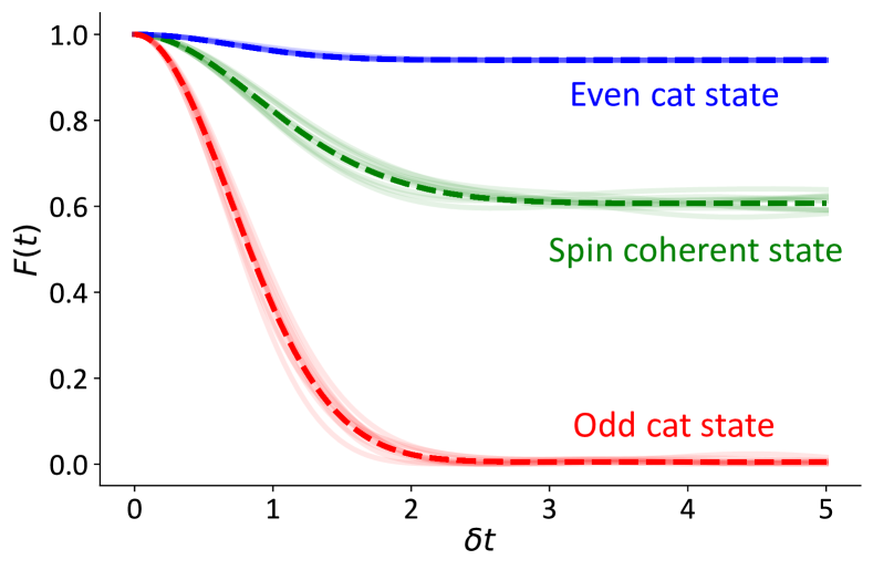
(a)

Figure 1: Fidelity $F(t)$ for spin coherent, even cat and odd cat states under the free evolution of the dephasing Hamiltonian $H_{0}$. The light solid lines depict the random realizations of the detunings (10 realizations shown), while the dashed lines correspond to the analytical result for the mean fidelity $\overline{F(t)}$. The parameters are $N=200$, $\theta=1/\sqrt{N}\approx 0.0707,\phi=0$.

III Parity-sensitive inhomogeneous dephasing

The spin coherent states are defined as

$$\ket{\theta,\phi}=\bigotimes_{n=1}^{N}\left(\cos\frac{\theta}{2}\ket{g_{n}}+e^{i\phi}\sin\frac{\theta}{2}\ket{e_{n}}\right).$$ (5)

Let us first consider the dynamics of the spin ensemble under the free evolution governed by the dephasing (inhomogeneous broadening) Hamiltonian $H_{0}=\sum_{n}\delta_{n}\sigma_{n}^{z}$. For concreteness, the detuning frequencies $\delta_{n}\sim\mathcal{N}(0,\delta^{2})$ are independently and identically distributed random variables drawn from a Gaussian distribution with zero mean and variance $\delta^{2}$. The overlap between the evolved state and the initial spin coherent state is given by

$$\begin{split}c(t)&\equiv\braket{\theta,\phi}{e^{-iH_{0}t}}{\theta,\phi}\\ &=\prod_{n=1}^{N}e^{i\delta_{n}t/2}\left(\cos\frac{\theta}{2}+e^{-i\delta_{n}t}\sin\frac{\theta}{2}\right).\end{split}$$ (6)

The fidelity $F(t)=|c(t)|^{2}$ indicates the survival probability of the initial state at time $t$. Using the Gaussian average $\mathbb{E}[\cos\delta_{n}t]=e^{-\delta^{2}t^{2}/2}$, we get the average fidelity

$$\overline{F(t)}=\left[1-\frac{1}{2}(1-e^{-\delta^{2}t^{2}/2})\sin^{2}\theta\right]^{N},$$ (7)

where the average is taken over random realizations of the frequencies $\delta_{n}$. In the weak excitation regime, $\theta$ is related to the amplitude of the bosonic coherent state via $|\alpha|\approx\sqrt{N}\tan(\theta/2)$ [27]. Hence, we make the small amplitude expansion $N\theta^{2}\ll 1$ to get

$$\overline{F(t)}=1-\frac{N\theta^{2}}{2}(1-e^{-\delta^{2}t^{2}/2})+O(N^{2}\theta^{4})$$ (8)

which implies $\overline{F(\infty)}\approx 1-(N\theta^{2})/2$ is of order unity since $N\theta^{2}\ll 1$. Using $\mathbb{E}[\cos^{2}\delta_{n}t]=(1+e^{-2\delta^{2}t^{2}})/2$, we can also evaluate the variance of the fidelity,

$$\text{Var}[F(t)]=\frac{N\theta^{4}}{8}(1-e^{-\delta^{2}t^{2}})+O(\theta^{6}).$$ (9)

Thus, the fluctuations of $F(t)$ are $\sim\sqrt{N}\theta^{2}$, which is much smaller than $\overline{F(t)}$. This implies that for sufficiently large systems, the random variable $F(t)$ concentrates around the mean $\overline{F(t)}$.

The spin cat states are defined as

$$\ket{\text{Cat}_{\pm}}=\frac{1}{\mathcal{N}_{\pm}}(\ket{\theta,\phi}\pm\ket{\theta,\phi+\pi}),$$ (10)

with the normalization factors

$$\mathcal{N}_{\pm}=\sqrt{2(1\pm\cos^{N}\theta)}.$$ (11)

As with the spin coherent states, we compute the fidelity of the cat states under the dephasing dynamics

$$F_{\pm}(t)\equiv|\braket{\text{Cat}_{\pm}}{e^{-iH_{0}t}}{\text{Cat}_{\pm}}|^{2}.$$ (12)

Using the Gaussian average $\mathbb{E}[\sin\delta_{n}t]=0$ from symmetry, and after some algebra, we obtain

$$\begin{split}\overline{F_{\pm}(t)}&=\frac{4}{\mathcal{N}_{\pm}^{4}}\bigg{[}\bigg{(}1-\frac{1}{2}(1-e^{-\delta^{2}t^{2}/2})\sin^{2}\theta\bigg{)}^{N}\\ &+\bigg{(}1-\frac{1}{2}(1+e^{-\delta^{2}t^{2}/2})\sin^{2}\theta\bigg{)}^{N}\pm 2\cos^{N}\theta\bigg{]}.\end{split}$$ (13)

In the small amplitude regime $N\theta^{2}\ll 1$ we obtain qualitatively different results for the even cat state

$$\overline{F_{+}(t)}=1-\frac{N^{2}\theta^{4}}{16}(1-e^{-\delta^{2}t^{2}})+O(N^{3}\theta^{6}),$$ (14)

and the odd cat state

$$\overline{F_{-}(t)}=e^{-\delta^{2}t^{2}}+O(N^{2}\theta^{4}).$$ (15)

The above expressions are simplified using $N\gg 1$. Note that the leading order term in Eq. (15) should be interpreted as the limiting case of $N\theta^{2}\to 0^{+}$, since $\theta=0$ is not well defined for the odd cat state. Similar to Eq. (9), one can also show that the relative fluctuations for the fidelity vanish as $N\to\infty$.

This reveals an important fact that the robustness of the cat state against inhomogeneous broadening is very sensitive to its parity symmetry. For the even cat state, the fidelity saturates at $F_{+}\approx 1-(N\theta^{2}/4)^{2}$ which is of order unity, while for the odd cat state the fidelity vanishes rapidly on the timescale of $\delta^{-1}$. Moreover, the even cat state is more robust than the spin coherent state, since the infidelity $1-\overline{F_{+}(t)}$ is quadratic in $N\theta^{2}$ (as compared to linear for the spin coherent state). Physically, this means that the dephasing effects are suppressed by even symmetry and amplified by odd symmetry.

III.1 Adding the stabilization dynamics

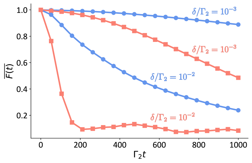
(a)

Figure 2: Mean fidelity $\overline{F(t)}$ under the full dissipative dynamics (1). The $N=8$ spins are initialized in the even (blue circles) and odd (red squares) cat states $\ket{\text{Cat}_{\pm}}$ with $\eta/\Gamma_{2}=0.2$, subject to inhomogeneous broadening with strengths $\delta/\Gamma_{2}=\{10^{-3},10^{-2}\}$. The fidelities are computed with respect to the initial state and averaged over $10$ realizations of the detunings. In the absence of inhomogeneous broadening, the fidelities of the steady states are $0.998$ (even) and $0.995$ (odd).

So far, we have only considered the free evolution governed by the dephasing Hamiltonian $H_{0}$. We now study numerically the full dissipative evolution governed by the master equation (1), using the QuTiP package [29]. Fig. 2 shows the mean fidelities $\overline{F(t)}$ for the cases of even and odd cat states, for $N=8$. In each case, we initialize the system in the even/odd cat state and measure the fidelity with respect to the initial state. In the absence of inhomogeneous broadening, the steady states achieve fidelities of $0.998$ and $0.995$ for the even and odd cat states respectively. We see that the odd cat state is significantly more susceptible to the dephasing effects. For example, at time $\Gamma_{2}t\approx 200$ with $\delta/\Gamma_{2}=10^{-2}$, the even cat state has a fidelity around $0.74$ while the fidelity of the odd cat state is only around $0.1$. This shows that the parity-sensitive dephasing derived for the simple case of only free Hamiltonian evolution applies even with the driven-dissipative stabilization terms. In Ref. [27], it was shown numerically that the even cat state $\ket{\text{Cat}_{+}}$ is robust against inhomogeneous broadening (and other imperfections). This is consistent with our findings. We argue here that the same robustness does not apply to the odd cat state, even at larger system sizes beyond the reach of numerical simulations. For larger $N$, one expects that the effects of inhomogeneous broadening are suppressed due to stronger collective interactions, but the separation of timescales in the fidelity decay between the even and odd cat state should remain valid.

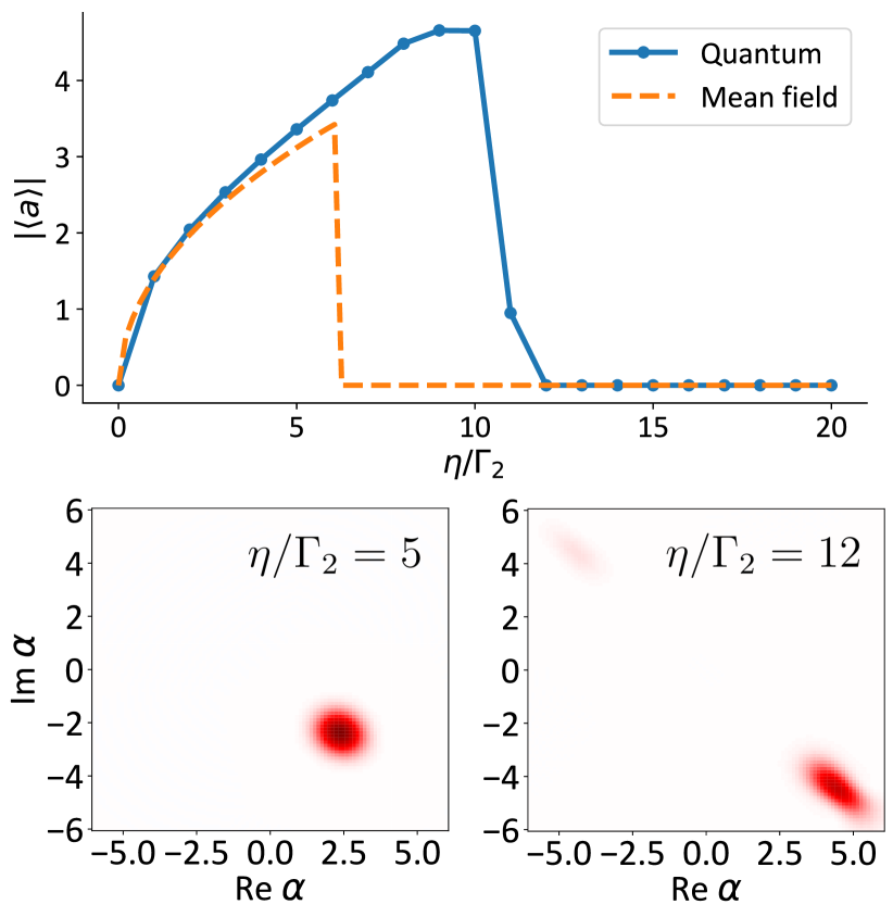
(a)

Figure 3: (Top) Steady state amplitude $|\braket{a}|$ against $\eta/\Gamma_{2}$ for the quantum model with $N=100$. The initial state is the bosonic coherent state with complex amplitude $\alpha=\sqrt{2\eta/\Gamma_{2}}e^{-i\pi/4}$. The dashed line corresponds to the mean field solution for $\sqrt{N}A$ in Eq. (19). (Bottom) Steady state Wigner functions for $\eta/\Gamma_{2}\in\{5,12\}$.

IV Mean-field analysis: Synchronization phase transition

Since a direct analytical treatment of Eq. (1) is not feasible, we consider instead a mean-field approximation where we assume a product state ansatz for $\rho$. The spin coherent state in Eq. (5) is a product state, so we expect this to be a reasonable approximation for large $N$. The mean-field equations can be physically interpreted as describing the synchronization dynamics of $N$ globally coupled classical spins, containing both dissipative and coherent (also called reactive) couplings. As we will show, this system exhibits a synchronization transition with both $\eta/\Gamma_{2}$ and $\delta/\Gamma_{2}$, where the spins become desynchronized beyond a critical parameter value. This provides important insights on the robustness of the spin coherent states to inhomogeneous broadening with driven-dissipative stabilization, for large system sizes.

The mean-field equations governing the dynamics of the $m$-th spin read (see Appendix A for a detailed derivation):

$$\begin{split}\frac{d}{dt}\braket{\sigma_{m}^{+}}&=i\delta_{m}\braket{\sigma_{m}^{+}}-2i\eta e^{i\theta}\braket{\sigma_{m}^{z}}c_{1,m}^{*}\\ &-2\Gamma_{2}\braket{\sigma_{m}^{+}}\left(\frac{c_{2,m}}{N}+|c_{1,m}|^{2}\right)\\ &+\Gamma_{2}\braket{\sigma_{m}^{z}}c_{1,m}(2c_{2,m}+N|c_{1,m}|^{2})\end{split}$$ (16)

and

$$\begin{split}\frac{d}{dt}\braket{\sigma_{m}^{z}}&=8\eta\text{Im}\left(e^{-i\theta}\braket{\sigma_{m}^{+}}c_{1,m}\right)\\ &-4\Gamma_{2}(1+\braket{\sigma_{m}^{z}})\left(\frac{c_{2,m}}{N}+|c_{1,m}|^{2}\right)\\ &-4\Gamma_{2}\text{Re}[\braket{\sigma_{m}^{+}}c_{1,m}^{*}(2c_{2}+N|c_{1,m}|^{2})]\end{split}$$ (17)

where $c_{1,m}\equiv\frac{1}{N}\sum_{j\neq m}\braket{\sigma_{j}^{+}}$ is the average coherence and $c_{2,m}\equiv\frac{1}{2N}\sum_{j\neq m}(1+\braket{\sigma_{j}^{z}})$ is the spin excitation density, excluding the $m$-th spin. Re and Im denote the real and imaginary parts respectively. The squeezing phase $\varphi$ is set to zero without loss of generality.

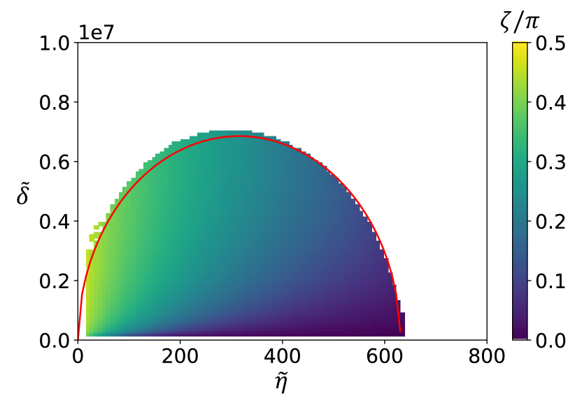
(a)

Figure 4: Steady state value of the phase spread $\zeta$ against the dimensionless detuning $\tilde{\delta}=N^{2}\delta/\Gamma_{2}$ and dimensionless squeezing $\tilde{\eta}=\eta/\Gamma_{2}$, for $N=10^{4}$ spins. The white region denote data points where the spins fail to converge to a synchronized state at long times. The red line marks the elliptical boundary of the synchronization region given by Eq. (22), with fitting parameters $a\approx 0.03125$ and $b\approx 2.2077$. For small values of $\tilde{\eta}$, some points within the synchronization region fail to converge to the steady state within the simulation time due to the slow dynamics.

IV.1 Identical frequencies

First, we consider the case where all the spins have the same frequency ($\delta=0$). This recovers the permutation symmetry in the system, which allows us to compare the mean-field solution to the exact quantum dynamics. From symmetry arguments, we denote $\braket{\sigma_{j}^{+}}=\braket{\sigma^{+}}=A\exp(i\phi)$ where $A$ and $\phi$ are to be determined, and $\braket{\sigma_{j}^{z}}=\braket{\sigma^{z}}=z$. Then, $c_{1,m}=(N-1)/N\times A\exp(i\phi)$ and $c_{2,m}=(N-1)/2N\times(1+z)$. This reduces the problem drastically from $3N$ real variables to just $3$ real variables $A$, $\phi$ and $z$. For large $N$, the reduced equations of motion become

$$\begin{split}\frac{\dot{A}}{A}&=-2\eta z\sin 2\phi-2\Gamma_{2}A^{2}+N\Gamma_{2}zA^{2}\\ \dot{\phi}&=-2\eta zA\cos 2\phi\\ \frac{\dot{z}}{A^{2}}&=8\eta\sin 2\phi-4\Gamma_{2}(1+z)-4\Gamma_{2}NA^{2}.\end{split}$$ (18)

In the low excitation limit, the steady state of the master equation (1) is approximately the bosonic coherent state with $|\braket{a}|=\sqrt{N}A=\sqrt{2\eta/\Gamma_{2}},z\approx-1,\phi=\pi/4$. This agrees with the steady state solution of Eq. (18):

$$\begin{split}A^{2}&\approx\frac{4\eta-1+\sqrt{1-\frac{16\eta}{N\Gamma_{2}}}}{2N}\\ \phi&=\pi/4\\ z&\approx-\frac{1+\sqrt{1-\frac{16\eta}{N\Gamma_{2}}}}{2}\end{split}$$ (19)

which is valid in the range $0\leq\eta/(N\Gamma_{2})\leq 1/16$. To leading order in $\eta/{N\Gamma_{2}}$, we recover $A^{2}=2\eta/N\Gamma_{2}$ and $z=-1$ which matches the quantum results in the low excitation limit. The solution in Eq. (19) describes the synchronized state where the spins are all phase locked to one another. The range of validity of this solution can be interpreted as the synchronization region, where the synchronization is broken at $\eta/(N\Gamma_{2})=1/16$. This sharp behavior in $\eta/\Gamma$ can also be understood for the quantum system. Making the exact Holstein-Primakoff transformation as introduced in Sec. II, we plot the steady state bosonic amplitude $|\braket{a}|$ in Fig. 3 for $N=100$ spins, initializing in the coherent state with complex amplitude $\alpha=\sqrt{2\eta/\Gamma_{2}}e^{-i\pi/4}$. For small $\eta/\Gamma_{2}$, the mean-field approximation agrees well with the quantum model. Interestingly, the bosonic amplitude increases and drops sharply at $\eta/\Gamma_{2}\approx 10$, although the drop occurs at a larger value of $\eta/\Gamma_{2}$ compared to the mean field model ($\eta/\Gamma=6.25$). In the quantum case, the drop in amplitude has a different physical interpretation: the bosonic Hilbert space has a dimension of $N+1$. Due to the boundedness of the quantum phase space, the bosonic amplitude cannot increase indefinitely with $\eta/\Gamma_{2}$ as $\sqrt{2\eta/\Gamma_{2}}$. Thus, for sufficiently large amplitudes, a secondary blob emerges in the Wigner function at a phase difference of $\pi$ and causing $|\braket{a}|$ to collapse. As a simple estimate, this collapse occurs when $\braket{a^{\dagger}a}\propto N$ such that the boundaries of the phase space become relevant. Since $\braket{a^{\dagger}a}\sim\eta/\Gamma_{2}$, the amplitude collapse occurs when $\eta/\Gamma_{2}\propto N$, the same scaling as the mean-field prediction (even though the exact values differ).

IV.2 Oppositely detuned sub-ensembles

Now, we break permutation symmetry by adding detunings to the spins. For analytical tractability, we consider two sub-ensembles, each with $N/2$ spins (assuming $N$ is even), with detunings $\pm\delta$. The results derived for this model should hold qualitatively for the more realistic model of random detunings (e.g., Gaussian distributed) which describes inhomogeneous broadening. Assuming that $\braket{\sigma^{+}}=A\exp[i(\pi/4\pm\zeta)]$ for the two sub-ensembles respectively, where $\zeta$ is the deviation of the phase from $\pi/4$, and $\braket{\sigma_{j}^{z}}=z$ for all spins, we can reduce the problem once again to just 3 nonlinear coupled equations

$$\begin{split}\frac{\dot{A}}{A}&=-2\eta z\left(\cos^{2}\zeta-\frac{1}{N}\cos 2\zeta\right)\\ &+\Gamma_{2}z\left(\cos^{2}\zeta-\frac{1}{N}\right)\left[1+z+NA^{2}\left(1-\frac{2}{N}\right)\cos^{2}\zeta\right]\\ \dot{\zeta}&=\delta+\eta z\left(1-\frac{2}{N}\right)\sin 2\zeta\\ &-\frac{\Gamma_{2}}{2}z\left[1+z+NA^{2}\left(1-\frac{2}{N}\right)\cos^{2}\zeta\right]\sin 2\zeta\\ \frac{\dot{z}}{A^{2}}&=8\eta\left(\cos^{2}\zeta-\frac{1}{N}\cos 2\zeta\right)\\ &-4\Gamma_{2}\left(\cos^{2}\zeta-\frac{1}{N}\right)\left[1+z+NA^{2}\left(1-\frac{2}{N}\right)\cos^{2}\zeta\right]\\ &-4\Gamma_{2}(1+z)\cos^{2}\zeta\end{split}$$ (20)

To verify the accuracy of Eq. (20), we compare numerical simulations of Eq. (20) with the full mean-field equations (16) and (17). It is also simple to see that this is consistent with Eq. (19) by setting $\delta=0,\phi\approx\pi/4,z\approx-1$ and taking the large $N$ limit.

Compared to the previous case of identical frequencies, this set of equations is much harder to solve analytically. For small $\zeta$, we can get an approximate solution by expanding Eq. (20) to first order in $\zeta$ and also first order in $1/N$, the approximate steady state solution corresponding to the synchronized state is (see Appendix B)

$$\begin{split}A^{2}&\approx\frac{4\eta-1+\sqrt{1-\frac{16\eta}{N\Gamma_{2}}}}{2N}\\ \zeta&\approx\frac{1+\sqrt{1-\frac{16\eta}{N\Gamma_{2}}}}{32\eta^{2}}N^{2}\Gamma_{2}\delta\\ z&\approx-\frac{1+\sqrt{1-\frac{16\eta}{N\Gamma_{2}}}}{2}\end{split}$$ (21)

This solution is valid for small $\delta$ (where the dephasing of the ensemble is slow) or large $\eta$ (where the synchronization effect is strong). For $\eta/N\Gamma_{2}\ll 1$, the formula for phase spread simplifies to $\zeta\approx N^{2}\Gamma_{2}\delta/16\eta^{2}$. Interestingly, while the phase spread is linear in $\delta$, the steady state values for $A^{2}$ and $z$ are independent of $\delta$ up to linear order.

For larger values of $\delta$, we perform numerical simulations of the mean-field equations for $N=10^{4}$ spins, shown in Fig. 4. The steady state value of the phase spread $\zeta$ is small for small $\delta$ and large $\eta$, which agrees with our physical intuition. For the case of identical frequencies $\delta=0$, there is a maximum $\eta/\Gamma_{2}$ of $N/16=625$ beyond which the synchronization breaks, agreeing with our analytical calculations. As $\delta$ increases, the region of synchronization narrows until a threshold value such that no synchronization is possible for any $\eta$. The boundary of the synchronization region appears to be elliptical. We postulate that the boundary curve takes the form

$$\tilde{\delta}=b\sqrt{a^{2}-(\tilde{\eta}-a)^{2}}$$ (22)

where $\tilde{\delta}\equiv N^{2}\delta/\Gamma_{2}$ and $\tilde{\eta}\equiv\eta/\Gamma_{2}$ are the dimensionless frequency detuning and squeezing respectively, and $a,b$ are the fitting parameters. The threshold values are thus $\tilde{\eta}_{c}=2a$ and $\tilde{\delta}_{c}=ab$. From numerical fitting, we find that $a\approx 0.03125$ and $b\approx 2.2077$ which gives $\tilde{\eta}_{c}\approx 0.0625N$ and $\tilde{\delta}_{c}\approx 0.06888N^{2}$. The value of $\tilde{\eta}_{c}$ agrees excellently with the theoretical prediction of $N/16$.

Since $\tilde{\delta}_{c}\propto N^{2}$, the critical detuning $\delta_{c}/\Gamma_{2}\approx 0.06888$ is independent of $N$. This suggests that the robustness of the spin coherent state to inhomogeneous broadening is independent of $N$, for a fixed $\eta/\Gamma_{2}$. Since the odd cat state is more fragile than the spin coherent state by the parity-sensitive dephasing effect, this supports the lack of robustness for the odd cat state, consistent with the numerical results in Fig. 2 for the quantum model.

V Discussion and Outlook

In this work, we analyze the effects of symmetry-breaking inhomogeneous dephasing on collective spin states such as spin coherent states and cat states $|\text{Cat}_{\pm}\rangle$ formed from the superposition of two spin coherent states offset by a $\pi$-phase. We show that the spin dephasing is highly sensitive to the parity symmetry of the collective spin state: For $|\text{Cat}_{+}\rangle$, even symmetry provides enhanced protection against inhomogeneous dephasing which grows with the system size $N$. On the contrary, the odd symmetry in $|\text{Cat}_{-}\rangle$ renders it significantly more fragile to inhomogeneous dephasing, causing the fidelity to decay rapidly.

This has important implications in using macroscopic spin ensembles as ‘cat qubits’ to encode logical quantum information, motivated by recent successful experiments in superconducting quantum circuits. Due to the collectively enhanced interactions in spin ensembles scaling as $\sqrt{N}$, they stand to benefit from greater error-correcting capabilities compared to their bosonic counterpart. However, using spin ensembles also come with a different set of experimental challenges like particle loss which has to be carefully addressed. In certain implementations such as rare-earth ions, inhomogeneous broadening arising from spatially-varying magnetic fields break permutation symmetry which is required for the spins to behave collectively, and causes spin dephasing. In Ref. [27], it was demonstrated explicitly that $|\text{Cat}_{+}\rangle$ is robust against such inhomogeneous dephasing, which is consistent with our results. However, our results also suggest that the odd cat state $|\text{Cat}_{-}\rangle$ is significantly more fragile. This means that the lifetime of $|\text{Cat}_{-}\rangle$ is limited by the dephasing timescale from the inhomogeneous broadening, which is on the order of $1$ $\mu\text{s}$ (taking $\delta\sim 1$ MHz). Consequently, encoding the logical qubit using $|\text{Cat}_{\pm}\rangle$ is unlikely to result in logical lifetimes significantly longer than the break-even point.

An alternative logical encoding is to define the basis states $\ket{0}_{L}\propto\ket{\theta,0}+\ket{\theta,\pi}$ and $\ket{1}_{L}\propto\ket{\theta,\pi/2}+\ket{\theta,3\pi/2}$, where $\ket{\theta,\phi}$ are the spin coherent states (5). Here, the logical qubit is encoded in the even parity subspace which enjoys the enhanced protection against inhomogeneous broadening. This encoding is analogous to the ‘four-legged cat code’ proposed in bosonic quantum error correction [30]. To stabilize this as the steady state, one approach would be to replace the collective two-body terms in Eq. (1) with collective four-body terms. However, it is very challenging in practice to implement quartic dissipators of the form $\mathcal{D}[S_{-}^{4}]\rho$, where $S_{-}$ is the collective spin lowering operator, while suppressing all unwanted dissipative terms.

Apart from quantum error correction, our results are also relevant for other applications of collective spin systems such as metrology and quantum simulation of dissipative phase transitions. As a future work, it would be interesting to study the parity-sensitive dephasing effect in more general dynamics beyond the specific master equation studied here, and also for general spin states with well-defined parity symmetry. One can also go beyond the product state ansatz and include quantum correlations in the numerical simulations using higher-order mean-field methods such as cumulant expansion [31, 32], which has been widely employed to study many-body spin dynamics [33, 34, 35, 36, 37, 38].

Appendix A Derivation of the semiclassical mean-field equations

Starting from the quantum master equation (1), we make the mean-field ansatz $\rho=\bigotimes_{i=1}^{N}\rho_{i}$ which assumes that the quantum correlations are negligible. This allows us to derive the single-spin dynamics for $\braket{\sigma_{m}^{+}}\equiv\text{Tr}(\sigma_{m}^{+}\rho_{m})$ and $\braket{\sigma_{m}^{z}}\equiv\text{Tr}(\sigma_{m}^{z}\rho_{m})$. Equivalently, we factorize spin correlations $\braket{\sigma_{i}^{+}\sigma_{j}^{-}}\approx\braket{\sigma_{i}^{+}}\braket{\sigma_{j}^{-}}$ and $\braket{\sigma_{i}^{+}\sigma_{i}^{-}\sigma_{j}^{-}}\approx\braket{\sigma_{i}^{+}\sigma_{i}^{-}}\braket{\sigma_{j}^{-}}=(1+\braket{\sigma_{i}^{z}})\braket{\sigma_{j}^{-}}/2$ for $i\neq j$. Note that we treat the population and coherence separately, i.e., we do not assume $\braket{\sigma_{i}^{+}\sigma_{i}^{-}}\approx\braket{\sigma_{i}^{+}}\braket{\sigma_{i}^{-}}$, which allows us to capture some effects of quantum coherence while the spins are weakly excited. The contributions from the squeezing Hamiltonian are

$$\frac{d}{dt}\braket{\sigma_{m}^{+}}=i\frac{\eta}{N}\sum_{i,j}e^{i\theta}\braket{[\sigma_{i}^{-}\sigma_{j}^{-},\sigma_{m}^{+}]}+e^{-i\theta}\cancel{\braket{[\sigma_{i}^{+}\sigma_{j}^{+},\sigma_{m}^{+}]}}=\frac{2i\eta}{N}e^{i\theta}\sum_{j\neq m}\braket{[\sigma_{m}^{-},\sigma_{m}^{+}]\sigma_{j}^{-}}\approx\frac{-2i\eta}{N}e^{i\theta}\braket{\sigma_{m}^{z}}\sum_{j\neq m}\braket{\sigma_{j}^{-}}$$ (23)

where the factor of 2 comes from the symmetry of $i\leftrightarrow j$. For $\braket{\sigma_{m}^{z}}$, we have

$$\begin{split}\frac{d}{dt}\braket{\sigma_{m}^{z}}&=\frac{i\eta}{N}\left\{\sum_{i,j}e^{i\theta}\braket{[\sigma_{i}^{-}\sigma_{j}^{-},\sigma_{m}^{z}]}+e^{-i\theta}\braket{[\sigma_{i}^{+}\sigma_{j}^{+},\sigma_{m}^{z}]}\right\}=\frac{2i\eta}{N}\left\{\sum_{j\neq m}e^{i\theta}\braket{[\sigma_{m}^{-},\sigma_{m}^{z}]\sigma_{j}^{-}}+e^{-i\theta}\braket{[\sigma_{m}^{+},\sigma_{m}^{z}]\sigma_{j}^{+}}\right\}\\ &\approx\frac{4i\eta}{N}\sum_{j\neq m}e^{i\theta}\braket{\sigma_{m}^{-}}\braket{\sigma_{j}^{-}}-e^{-i\theta}\braket{\sigma_{m}^{+}}\braket{\sigma_{j}^{+}}=\frac{8\eta}{N}\text{Im}\left(e^{-i\theta}\braket{\sigma_{m}^{+}}\sum_{j\neq m}\braket{\sigma_{j}^{+}}\right).\end{split}$$ (24)

Next, we compute the contribution from the collective two-body dissipator

$$\begin{split}\frac{N^{2}}{\Gamma_{2}}\frac{d}{dt}\braket{\sigma_{m}^{+}}&=\sum_{i,j,k,l}\braket{\sigma_{i}^{+}\sigma_{j}^{+}\sigma_{m}^{+}\sigma_{k}^{-}\sigma_{l}^{-}-\frac{1}{2}\sigma_{m}^{+}\sigma_{i}^{+}\sigma_{j}^{+}\sigma_{k}^{-}\sigma_{l}^{-}-\frac{1}{2}\sigma_{i}^{+}\sigma_{j}^{+}\sigma_{k}^{-}\sigma_{l}^{-}\sigma_{m}^{+}}\\ &\approx\braket{\sigma_{m}^{+}\sigma_{m}^{-}}\sum_{\begin{subarray}{c}i,j,k\\ ijk\neq m\end{subarray}}\braket{\sigma_{i}^{+}\sigma_{j}^{+}\sigma_{k}^{-}}-\braket{\sigma_{m}^{-}\sigma_{m}^{+}}\sum_{\begin{subarray}{c}i,j,k\\ ijk\neq m\end{subarray}}\braket{\sigma_{i}^{+}\sigma_{j}^{+}\sigma_{k}^{-}}-2\braket{\sigma_{m}^{+}\sigma_{m}^{-}\sigma_{m}^{+}}\sum_{\begin{subarray}{c}i,j\\ ij\neq m\end{subarray}}\braket{\sigma_{i}^{+}\sigma_{j}^{-}}\\ &=\braket{\sigma_{m}^{z}}\sum_{\begin{subarray}{c}i,j,k\\ ijk\neq m\end{subarray}}\braket{\sigma_{i}^{+}\sigma_{j}^{+}\sigma_{k}^{-}}-2\braket{\sigma_{m}^{+}}\sum_{\begin{subarray}{c}i,j\\ ij\neq m\end{subarray}}\braket{\sigma_{i}^{+}\sigma_{j}^{-}}\end{split}$$ (25)

Eq. (25) contains terms such as $\braket{\sigma_{i}^{+}\sigma_{j}^{+}\sigma_{k}^{-}}$ and $\braket{\sigma_{i}^{+}\sigma_{j}^{-}}$. To obtain a closed set of mean-field equations, we have to reduce these in terms of $\braket{\sigma_{i}^{+}}$ and $\braket{\sigma_{i}^{z}}$. Defining $c_{1,m}\equiv\frac{1}{N}\sum_{j\neq m}\braket{\sigma_{j}^{+}}$ and $c_{2,m}\equiv\frac{1}{2N}\sum_{j\neq m}(1+\braket{\sigma_{j}^{z}})$, we then obtain

$$\begin{split}\frac{N^{2}}{\Gamma_{2}}\frac{d}{dt}\braket{\sigma_{m}^{+}}&\approx\braket{\sigma_{m}^{z}}\left(2\sum_{\begin{subarray}{c}i,j\\ ij\neq m\\ i\neq j\end{subarray}}\braket{\sigma_{i}^{+}\sigma_{i}^{-}}\braket{\sigma_{j}^{+}}+\sum_{\begin{subarray}{c}i,j,k\\ ijk\neq m\\ i\neq j\neq m\end{subarray}}\braket{\sigma_{i}^{+}}\braket{\sigma_{j}^{+}}\braket{\sigma_{k}^{-}}\right)-2\braket{\sigma_{m}^{+}}\left(\sum_{i\neq m}\braket{\sigma_{i}^{+}\sigma_{i}^{-}}+\sum_{\begin{subarray}{c}i,j\\ ij\neq m\\ i\neq j\end{subarray}}\braket{\sigma_{i}^{+}}\braket{\sigma_{j}^{-}}\right)\\ &=-2\braket{\sigma_{m}^{+}}(Nc_{2,m}+N^{2}|c_{1,m}|^{2})+\braket{\sigma_{m}^{z}}(2N^{2}c_{1,m}c_{2,m}+N^{3}|c_{1,m}|^{2}c_{1,m})\end{split}$$ (26)

Similarly, we can obtain the equation of motion for $\braket{\sigma_{m}^{z}}$:

$$\begin{split}\frac{1}{\Gamma_{2}}\frac{d}{dt}\braket{\sigma_{m}^{z}}&=\sum_{i,j,k,l}\braket{\sigma_{i}^{+}\sigma_{j}^{+}\sigma_{m}^{z}\sigma_{k}^{-}\sigma_{l}^{-}-\frac{1}{2}\sigma_{m}^{z}\sigma_{i}^{+}\sigma_{j}^{+}\sigma_{k}^{-}\sigma_{l}^{-}-\frac{1}{2}\sigma_{i}^{+}\sigma_{j}^{+}\sigma_{k}^{-}\sigma_{l}^{-}\sigma_{m}^{z}}\\ &\approx(\braket{\sigma_{m}^{+}\sigma_{m}^{z}}-\braket{\sigma_{m}^{z}\sigma_{m}^{+}})\sum_{\begin{subarray}{c}i,j,k\\ ijk\neq m\end{subarray}}\braket{\sigma_{i}^{+}\sigma_{j}^{-}\sigma_{k}^{-}}+(\braket{\sigma_{m}^{z}\sigma_{m}^{-}}-\braket{\sigma_{m}^{-}\sigma_{m}^{z}}\sum_{\begin{subarray}{c}i,j,k\\ ijk\neq m\end{subarray}}\braket{\sigma_{i}^{+}\sigma_{j}^{+}\sigma_{k}^{-}}\\ &+(4\braket{\sigma_{m}^{+}\sigma_{m}^{z}\sigma_{m}^{-}}-2\braket{\sigma_{m}^{z}\sigma_{m}^{+}\sigma_{m}^{-}}-2\braket{\sigma_{m}^{+}\sigma_{m}^{-}\sigma_{m}^{z}})\sum_{\begin{subarray}{c}i,j\\ ij\neq m\end{subarray}}\braket{\sigma_{i}^{+}\sigma_{j}^{-}}\\ &=-2\braket{\sigma_{m}^{+}}\sum_{\begin{subarray}{c}i,j,k\\ ijk\neq m\end{subarray}}\braket{\sigma_{i}^{+}\sigma_{j}^{-}\sigma_{k}^{-}}-2\braket{\sigma_{m}^{-}}\sum_{\begin{subarray}{c}i,j,k\\ ijk\neq m\end{subarray}}\braket{\sigma_{i}^{+}\sigma_{j}^{+}\sigma_{k}^{-}}-4(1+\braket{\sigma_{m}^{z}})\sum_{\begin{subarray}{c}i,j\\ ij\neq m\end{subarray}}\braket{\sigma_{i}^{+}\sigma_{j}^{-}}\\ &=-4\text{Re}\left(\braket{\sigma_{m}^{+}}\sum_{\begin{subarray}{c}i,j,k\\ ijk\neq m\end{subarray}}\braket{\sigma_{i}^{+}\sigma_{j}^{-}\sigma_{k}^{-}}\right)-4(1+\braket{\sigma_{m}^{z}})\sum_{\begin{subarray}{c}i,j\\ ij\neq m\end{subarray}}\braket{\sigma_{i}^{+}\sigma_{j}^{-}}\\ &\approx-4\text{Re}\left[\braket{\sigma_{m}^{+}}\left(2\sum_{\begin{subarray}{c}i,j\\ ij\neq m\\ i\neq j\end{subarray}}\braket{\sigma_{i}^{+}\sigma_{i}^{-}}\braket{\sigma_{j}^{-}}+\sum_{\begin{subarray}{c}i,j,k\\ ijk\neq m\\ i\neq j\neq k\end{subarray}}\braket{\sigma_{i}^{+}}\braket{\sigma_{j}^{-}}\braket{\sigma_{k}^{-}}\right)\right]-4(1+\braket{\sigma_{m}^{z}})\left(\sum_{i\neq m}\braket{\sigma_{i}^{+}\sigma_{i}^{-}}+\sum_{\begin{subarray}{c}i,j\\ ij\neq m\end{subarray}}\braket{\sigma_{i}^{+}}\braket{\sigma_{j}^{-}}\right)\\ &=-4(1+\braket{\sigma_{m}^{z}})(Nc_{2,m}+N^{2}|c_{1,m}|^{2})+\text{Re}[\braket{\sigma_{m}^{z}}(2N^{2}c_{1,m}^{*}c_{2,m}+N^{3}|c_{1,m}|^{2}c_{1,m}^{*}]\end{split}$$ (27)

Combining Eqs. (23), (24), (26) and (27), we have the mean-field equations:

$$\begin{split}\frac{d}{dt}\braket{\sigma_{m}^{+}}&=i\omega_{m}\braket{\sigma_{m}^{+}}-2i\eta e^{i\theta}\braket{\sigma_{m}^{z}}c_{1,m}^{*}-2\Gamma_{2}\braket{\sigma_{m}^{+}}\left(\frac{c_{2,m}}{N}+|c_{1,m}|^{2}\right)+\Gamma_{2}\braket{\sigma_{m}^{z}}c_{1,m}(2c_{2,m}+N|c_{1,m}|^{2})\end{split}$$ (28)

$$\begin{split}\frac{d}{dt}\braket{\sigma_{m}^{z}}&=8\eta\text{Im}\left(e^{-i\theta}\braket{\sigma_{m}^{+}}c_{1,m}\right)-4\Gamma_{2}(1+\braket{\sigma_{m}^{z}})\left(\frac{c_{2,m}}{N}+|c_{1,m}|^{2}\right)-4\Gamma_{2}\text{Re}[\braket{\sigma_{m}^{+}}c_{1,m}^{*}(2c_{2}+N|c_{1,m}|^{2})]\end{split}$$ (29)

as described in Eqs. (16) and (17) in the main text.

Appendix B Two detuned ensembles, small $\delta$ limit

When the detuning $\delta$ is small, we expect the steady state value for the phase $\phi$ to be close to $\pi/4$, as was shown in Eq. (19). Writing $\phi=\pi/4\pm\zeta$, we obtain the mean-field equations (20). Expanding the equations to linear order in $\zeta$, and then to order $1/N$, we obtain the simplifed equations (setting $\Gamma_{2}=1$ for notational simplicity)

$$\begin{split}\frac{\dot{A}}{A}&\approx-2A^{2}+\frac{N-1}{N}z(1-2\eta+(N-2)A^{2})+\frac{N-1}{N}z^{2}\\ \dot{\zeta}&\approx\delta-\frac{z}{N}(N+4\eta-2N\eta+(N-2)A^{2}+Nz)\zeta\\ \frac{\dot{z}}{A^{2}}&\approx\frac{4A^{2}}{N}(1+2N(\eta-1)-2\eta-(N-2)(N-1)A^{2}+z-2Nz).\end{split}$$ (30)

Since $A^{2}$ is of order $1/N$, one has to be careful here when making the large $N$ approximation. We verify the accuracy of the above equation by comparing numerical simulations against those from the full mean-field equations (16) and (17). The steady state solution is complicated, but we can expand in powers of $1/N$ to get

$$A^{2}\approx\frac{2\eta}{N}-\frac{4\eta}{N^{2}}+\frac{4\eta-32\eta^{2}}{N^{2}}+\ldots\approx\frac{2\eta}{N},$$ (31)

$$\zeta\approx\delta\left(\frac{1+\sqrt{1-16(\eta/N)}}{32(\eta/N)^{2}}+\frac{1+32(\eta/N)}{128N(\eta/N)^{3}}+\ldots\right)\approx\frac{1+\sqrt{1-16\eta/N}}{32(\eta/N)^{2}}\delta$$ (32)

and

$$z\approx-\frac{1+\sqrt{1-16\eta/N}}{2}$$ (33)

References

- Pezzè et al. [2018] L. Pezzè, A. Smerzi, M. K. Oberthaler, R. Schmied, and P. Treutlein, Quantum metrology with nonclassical states of atomic ensembles, Rev. Mod. Phys. 90, 035005 (2018).
- Zhou et al. [2020] H. Zhou, J. Choi, S. Choi, R. Landig, A. M. Douglas, J. Isoya, F. Jelezko, S. Onoda, H. Sumiya, P. Cappellaro, H. S. Knowles, H. Park, and M. D. Lukin, Quantum metrology with strongly interacting spin systems, Phys. Rev. X 10, 031003 (2020).
- Arunkumar et al. [2023] N. Arunkumar, K. S. Olsson, J. T. Oon, C. A. Hart, D. B. Bucher, D. R. Glenn, M. D. Lukin, H. Park, D. Ham, and R. L. Walsworth, Quantum logic enhanced sensing in solid-state spin ensembles, Phys. Rev. Lett. 131, 100801 (2023).
- Wesenberg et al. [2009] J. H. Wesenberg, A. Ardavan, G. A. D. Briggs, J. J. L. Morton, R. J. Schoelkopf, D. I. Schuster, and K. Mølmer, Quantum computing with an electron spin ensemble, Phys. Rev. Lett. 103, 070502 (2009).
- Brion et al. [2007] E. Brion, K. Mølmer, and M. Saffman, Quantum computing with collective ensembles of multilevel systems, Phys. Rev. Lett. 99, 260501 (2007).
- Barrett et al. [2010] S. D. Barrett, P. P. Rohde, and T. M. Stace, Scalable quantum computing with atomic ensembles, New J. Phys. 12, 093032 (2010).
- Georgescu et al. [2014] I. M. Georgescu, S. Ashhab, and F. Nori, Quantum simulation, Rev. Mod. Phys. 86, 153 (2014).
- Islam et al. [2011] R. Islam, E. E. Edwards, K. Kim, S. Korenblit, C. Noh, H. Carmichael, G.-D. Lin, L.-M. Duan, C.-C. Joseph Wang, J. K. Freericks, and C. Monroe, Onset of a quantum phase transition with a trapped ion quantum simulator, Nat. Commun. 2, 377 (2011).
- Koppenhöfer et al. [2022] M. Koppenhöfer, P. Groszkowski, H.-K. Lau, and A. Clerk, Dissipative superradiant spin amplifier for enhanced quantum sensing, PRX Quantum 3, 030330 (2022).
- Duan et al. [2001] L.-M. Duan, M. D. Lukin, J. I. Cirac, and P. Zoller, Long-distance quantum communication with atomic ensembles and linear optics, Nature 414, 413 (2001).
- Sangouard et al. [2011] N. Sangouard, C. Simon, H. de Riedmatten, and N. Gisin, Quantum repeaters based on atomic ensembles and linear optics, Rev. Mod. Phys. 83, 33 (2011).
- Dicke [1954] R. H. Dicke, Coherence in spontaneous radiation processes, Phys. Rev. 93, 99 (1954).
- Gross and Haroche [1982] M. Gross and S. Haroche, Superradiance: An essay on the theory of collective spontaneous emission, Phys. Rep. 93, 301 (1982).
- Masson et al. [2020] S. J. Masson, I. Ferrier-Barbut, L. A. Orozco, A. Browaeys, and A. Asenjo-Garcia, Many-body signatures of collective decay in atomic chains, Phys. Rev. Lett. 125, 263601 (2020).
- Masson and Asenjo-Garcia [2022] S. J. Masson and A. Asenjo-Garcia, Universality of dicke superradiance in arrays of quantum emitters, Nat. Commun. 13, 2285 (2022).
- Sierra et al. [2022] E. Sierra, S. J. Masson, and A. Asenjo-Garcia, Dicke superradiance in ordered lattices: Dimensionality matters, Phys. Rev. Research 4, 023207 (2022).
- Robicheaux [2021] F. Robicheaux, Theoretical study of early-time superradiance for atom clouds and arrays, Phys. Rev. A 104, 063706 (2021).
- Malz et al. [2022] D. Malz, R. Trivedi, and J. I. Cirac, Large- limit of dicke superradiance, Phys. Rev. A 106, 013716 (2022).
- Cardenas-Lopez et al. [2023] S. Cardenas-Lopez, S. J. Masson, Z. Zager, and A. Asenjo-Garcia, Many-body superradiance and dynamical mirror symmetry breaking in waveguide qed, Phys. Rev. Lett. 131, 033605 (2023).
- Mok et al. [2023] W.-K. Mok, A. Asenjo-Garcia, T. C. Sum, and L.-C. Kwek, Dicke superradiance requires interactions beyond nearest neighbors, Phys. Rev. Lett. 130, 213605 (2023).
- Rainò et al. [2020] G. Rainò, H. Utzat, M. Bawendi, and M. Kovalenko, Superradiant emission from self-assembled light emitters: From molecules to quantum dots, MRS Bulletin 45, 841–848 (2020).
- Rainò et al. [2018] G. Rainò, M. A. Becker, M. I. Bodnarchuk, R. F. Mahrt, M. V. Kovalenko, and T. Stöferle, Superfluorescence from lead halide perovskite quantum dot superlattices, Nature 563, 671 (2018).
- Lei et al. [2023] M. Lei, R. Fukumori, J. Rochman, B. Zhu, M. Endres, J. Choi, and A. Faraon, Many-body cavity quantum electrodynamics with driven inhomogeneous emitters, Nature 617, 271 (2023).
- Leghtas et al. [2015] Z. Leghtas, S. Touzard, I. M. Pop, A. Kou, B. Vlastakis, A. Petrenko, K. M. Sliwa, A. Narla, S. Shankar, M. J. Hatridge, M. Reagor, L. Frunzio, R. J. Schoelkopf, M. Mirrahimi, and M. H. Devoret, Confining the state of light to a quantum manifold by engineered two-photon loss, Science 347, 853 (2015).
- Lescanne et al. [2020] R. Lescanne, M. Villiers, T. Peronnin, A. Sarlette, M. Delbecq, B. Huard, T. Kontos, M. Mirrahimi, and Z. Leghtas, Exponential suppression of bit-flips in a qubit encoded in an oscillator, Nat. Phys. 16, 509 (2020).
- Radcliffe [1971] J. M. Radcliffe, Some properties of coherent spin states, J. Phys. A: Gen. Phys. 4, 313 (1971).
- Qin et al. [2021] W. Qin, A. Miranowicz, H. Jing, and F. Nori, Generating long-lived macroscopically distinct superposition states in atomic ensembles, Phys. Rev. Lett. 127, 093602 (2021).
- Mirrahimi et al. [2014] M. Mirrahimi, Z. Leghtas, V. V. Albert, S. Touzard, R. J. Schoelkopf, L. Jiang, and M. H. Devoret, Dynamically protected cat-qubits: a new paradigm for universal quantum computation, New J. Phys. 16, 045014 (2014).
- Johansson et al. [2013] J. Johansson, P. Nation, and F. Nori, QuTiP 2: A python framework for the dynamics of open quantum systems, Comput. Phys. Commun. 184, 1234 (2013).
- Leghtas et al. [2013] Z. Leghtas, G. Kirchmair, B. Vlastakis, R. J. Schoelkopf, M. H. Devoret, and M. Mirrahimi, Hardware-efficient autonomous quantum memory protection, Phys. Rev. Lett. 111, 120501 (2013).
- Kubo [1962] R. Kubo, Generalized cumulant expansion method, J. Phys. Soc. Jpn. 17, 1100 (1962).
- Plankensteiner et al. [2022] D. Plankensteiner, C. Hotter, and H. Ritsch, QuantumCumulants.jl: A Julia framework for generalized mean-field equations in open quantum systems, Quantum 6, 617 (2022).
- Hotter et al. [2023] C. Hotter, L. Ostermann, and H. Ritsch, Cavity sub- and superradiance for transversely driven atomic ensembles, Phys. Rev. Res. 5, 013056 (2023).
- Debnath et al. [2018] K. Debnath, Y. Zhang, and K. Mølmer, Lasing in the superradiant crossover regime, Phys. Rev. A 98, 063837 (2018).
- Debnath et al. [2019] K. Debnath, Y. Zhang, and K. Mølmer, Collective dynamics of inhomogeneously broadened emitters coupled to an optical cavity with narrow linewidth, Phys. Rev. A 100, 053821 (2019).
- Debnath et al. [2020] K. Debnath, G. Dold, J. J. L. Morton, and K. Mølmer, Self-stimulated pulse echo trains from inhomogeneously broadened spin ensembles, Phys. Rev. Lett. 125, 137702 (2020).
- Rubies-Bigorda et al. [2023] O. Rubies-Bigorda, S. Ostermann, and S. F. Yelin, Characterizing superradiant dynamics in atomic arrays via a cumulant expansion approach, Phys. Rev. Res. 5, 013091 (2023).
- Masson et al. [2024] S. J. Masson, J. P. Covey, S. Will, and A. Asenjo-Garcia, Dicke superradiance in ordered arrays of multilevel atoms, PRX Quantum 5, 010344 (2024).