Towards Cooperative Maneuver Planning
in Mixed Traffic at Urban Intersections

Abstract

Connected automated driving promises a significant improvement of traffic efficiency and safety on highways and in urban areas. Apart from sharing of awareness and perception information over wireless communication links, cooperative maneuver planning may facilitate active guidance of connected automated vehicles at urban intersections. Research in automatic intersection management put forth a large body of works that mostly employ rule-based or optimization-based approaches primarily in fully automated simulated environments. In this work, we present two cooperative planning approaches that are capable of handling mixed traffic, i.e., the road being shared by automated vehicles and regular vehicles driven by humans. Firstly, we propose an optimization-based planner trained on real driving data that cyclically selects the most efficient out of multiple predicted coordinated maneuvers. Additionally, we present a cooperative planning approach based on graph-based reinforcement learning, which conquers the lack of ground truth data for cooperative maneuvers. We present evaluation results of both cooperative planners in high-fidelity simulation and real-world traffic. Simulative experiments in fully automated traffic and mixed traffic show that cooperative maneuver planning leads to less delay due to interaction and a reduced number of stops. In real-world experiments with three prototype connected automated vehicles in public traffic, both planners demonstrate their ability to perform efficient cooperative maneuvers.

6.8in(0.85in,0.15in) SUBMITTED TO REVIEW AND POSSIBLE PUBLICATION. COPYRIGHT WILL BE TRANSFERRED WITHOUT NOTICE.
Personal use of this material is permitted. Permission must be obtained for all other uses, in any current or future media, including reprinting/republishing this material for advertising or promotional purposes, creating new collective works, for resale or redistribution to servers or lists, or reuse of any copyrighted component of this work in other works.

I Introduction

Urban traffic is prone to inefficiencies and disturbances due to the ever increasing volume of traffic. This manifests, e.g., at smaller intersections, where static priority rules are the prevailing method for coordination of vehicles. Occlusions through buildings or other road users limit the field of view for both human drivers and vehicle-bound sensors of an automated vehicle (AV). Connected automated driving opens up new opportunities to improve urban traffic efficiency by leveraging communication links between vehicles and possibly infrastructure systems. Moreover, edge computing resources are becoming available in urban areas that enable, e.g., populating and maintaining a collective environment model (EM) of an area of interest. This setup allows connected automated vehicles (CAVs) to improve their local planning algorithms by incorporating data from the server-side EM, as it was shown in [1] at a suburban three-way intersection in Ulm-Lehr, Germany.

Figure 1: Cooperative maneuver at an urban intersection. The CAV $\nu_{3}$ on the major road gives way to the turning CAV $\nu_{1}$ and the CAV $\nu_{2}$ on the minor road under consideration of the HDV (gray). We propose an optimizing planner and an RL-based planner for deployment on an edge server.

In the current work, we build upon this approach and investigate the potential of cooperative maneuver planning, as illustrated in Fig. 1. By planning such maneuvers on a centralized instance, like an edge server, CAVs can be instructed to explicitly deviate from priority rules to reach peak efficiency. Urban automotive traffic will not be fully automated in the near future. Instead, mixed traffic, i.e., the simultaneous use of roads by both human-driven vehicles (HDVs) and AVs, will be prevalent. Therefore, any cooperative planner must consider HDVs that cannot be directly influenced and behave according to the priority rules. We present two approaches to cooperative maneuver planning, one of which leverages a fast long-term multi-scenario prediction to derive an optimal maneuver, based on [2]. The second approach employs reinforcement learning (RL) to train a graph neural network (GNN) policy for cooperative maneuver planning [3]. The execution of the cooperative maneuvers in both cases is based on the coordination protocol proposed in [4]. In principle, also connected vehicles (CVs) that are driven by a human can be included in the maneuver coordination scheme. Such an application is not in focus for this paper, though. The core contribution of the present work is twofold:

• Statistical analysis and comparison of both approaches in a new holistic simulation framework for fully automated and mixed traffic;

• Demonstration of the real-world applicability of both approaches using three prototypical CAVs.

The remainder of the paper is structured as follows: Section II discusses the state of the art in classical and learning-based cooperative planning for automated driving. The proposed optimization-based maneuver planner is introduced in Sec. IV, followed by the RL-based one in Sec. V. Afterwards, we present simulative evaluation results (Sec. VI) and our real-world experiments in public traffic (Sec. VII). Finally, Sec. VIII summarizes the results of the article and gives an outlook on future work.

II Related Work

The efficient coordination of CAVs at urban intersections receives strong research interest in the field of automatic intersection management (AIM). Prior works mostly consider fully automated traffic and simulative evaluations, as surveyed by [5]. In the following, we give an overview on published works that are deemed most relevant to cooperative maneuver planning in mixed traffic.

Static priority rules at an intersection can be insufficient to efficiently handle a higher amount of incoming traffic and lead to long queues. Instead, usually traffic lights are used as a basic means of traffic control. The traffic light switching plan can either be determined offline, potentially optimized for the specific intersection as in [6], or adapted dynamically with a Markovian approach as in [7]. With an increasing prevalence of connected vehicles, however, the traffic at intersections can be governed by an automatic intersection management. With a fine-grained control by controlling individual vehicles, the traffic efficiency can potentially be increased compared to simpler solutions.

Many authors focus on a simpler scenario with a full deployment of only CAVs. The enumeration of all possible vehicle crossing orders as in [8] yields to the optimal ordering. However, the number of order combinations is exponential in the number of vehicles as shown in [9]. Therefore, that method is not feasible in a real-time system and a more efficient algorithm needs to evaluate only the most promising combinations. A straightforward approach is to use a heuristics to directly generate a single crossing order. One of the earliest proposed heuristics is a first-come, first-served scheme to reserve cells in a discretized space-time grid for each vehicle, which was used by Dresner and Stone in [10], by Wuthishuwong and Trächtler in [11], and others. Another heuristics-like decentralized solution for two crossing vehicles is presented in [12]. In that work, the planned vehicle trajectories are compared and the intersection management logic only intervenes as little as possible to prevent a collision.

On the other hand, some approaches try to find a near-optimal crossing order of the arriving vehicles using more elaborated algorithms. Possible optimizing strategies are dynamic programming [13], a control policy based on Petri Nets [14], or Mixed Integer Quadratic Programs [15]. In some works, the tree structure of the chronological right of way decisions between vehicles is exploited and the optimal solution is searched using branch and bound [16] or Monte Carlo Tree Search [17].

Although non-learning approaches are still prevalent in AIM, machine learning is also gaining traction in connected automated driving. In [18], it is proposed to leverage collective perception to improve the performance of local planning algorithms. The planning task only considers one AV without cooperative objective, though. Due to lack of ground-truth data for training, learning-based approaches to AIM typically rely on RL. Such a learning-based approach is proposed by [19] that suggests to train a policy through RL to choose from a restricted action space that ensures collision-free maneuvers. Cooperative maneuvers can only be initiated implicitly by vehicle behavior because there is no explicit communication between the involved vehicles. In our previous works [20, 21], we have proposed a flexible graph-based scene representation and an RL training scheme for AIM in fully automated traffic. It was shown that the model outperforms a FIFO baseline and generalizes within certain limits to intersection layouts not encountered during training.

Fewer researchers have tackled the intersection management task for much more challenging mixed traffic and especially scenarios with a vast majority of HDVs, which will be prevalent in the near future. Dresner and Stone extended their cell reservation system from previous works by different fallback modes in [22]. Those modes use dynamically controlled traffic light phases to allow safe crossing of HDVs, which still provides comparable efficiency results at a rate of $5\text{\,}\frac{\mathrm{\char 37\relax}}{}$ HDVs. Bento et al. employ a similar system that switches traffic lights to green for individual vehicles [23]. Their system reserves cells for HDVs on all possible turning lanes assuming a velocity interval to predict the maximum intersection occupancy intervals, which works well for a low percentage of HDVs. Commonly, the gains of approaches for mostly CAV traffic deteriorate in an environment with a lot of HDVs.

The approach proposed in our previous work in [2], which we extended for this paper, is specifically designed to also work with a high HDV rate. It employs a multi-scenario prediction represented in a probabilistic decision tree and optimizes the expected efficiency by maneuvers between the present CAVs. Thereby, already a deployment rate of $40\text{\,}\frac{\mathrm{\char 37\relax}}{}$ CAVs yields to a noticeable overall efficiency gain which also benefits the HDVs.

In [24], the authors propose an RL approach assuming that automated vehicles only perceive their immediate surroundings. The RL policy is shown to manage intersection traversals in presence of simulated human-driven vehicles while turning maneuvers are disallowed. A further RL framework that combines local observations with a joint reward to accommodate a cooperative objective was presented by [25]. Although this model is capable of handling mixed traffic, the network architecture limits the maximum number of cooperating vehicles in the scene. Our RL-based cooperative planning model has been extended to mixed traffic in [3]. In addition, the integration of the trained RL policy with a sampling-based motion planner was addressed in [26]. The applicability to a real test vehicle was shown in experiments on a test track.

III Cooperative Maneuver Planning Module

In our proposed system architecture, the centralized cooperative planning module on the edge server plans a joint maneuver on behavior level, which is distributed to all CAVs in the scene using the protocol proposed in [4]. Each of the CAVs runs a local motion planner to derive a viable trajectory. Typical motion planning algorithms require a specification of the desired motion for a sufficient planning horizon (at least multiple seconds) into the future. Therefore, the distributed maneuver representation shall enable the vehicles to individually plan their trajectory locally.

Basis for the planning of cooperative maneuvers is the server-side EM. This EM is the result of fusing multiple data sources, like cooperative awareness messages (CAM, [27]) and collective perception messages (CPM, [28]) from connected vehicles or infrastructure perception [1]. Thus, the server-side EM is more extensive than the individual CAVs’ ones and is considered to contain all information relevant for maneuver planning. A vehicle in the EM is denoted as

$$\nu_{\mathrm{id}}=(\boldsymbol{T},\,v,\,\mathcal{D},\,c)\in\mathrm{EM},$$ (1)

where $\mathrm{id}$ denotes a unique identifier and the binary flag $c$ determines whether the vehicle is a CAV and thus controllable. $\boldsymbol{T}$ describes the vehicle’s pose on the local 2D ground plane and $v$ is the current driving speed. CAVs share their intended route or destination $\mathcal{D}$, which is unknown for HDVs, though, which are assumed to be non-connected.

The derived maneuvers are passed to the CAVs according to the maneuver coordination protocol proposal in [4]. While the proposed protocol is very generic and supports multiple cooperative use cases, we focus on the components that are relevant for AIM. Thus, the final step to provide the planned cooperative maneuver to the CAVs is to derive so-called longitudinal maneuver waypoints defined as

$$\mu_{\mathrm{id}}=(\boldsymbol{p},\,t_{\mathrm{min}},\,t_{\mathrm{max}},\,\nu^{\uparrow},\,\nu^{\downarrow})\in\mathcal{M},$$ (2)

where its position is given by $\boldsymbol{p}$. The interval $[t_{\mathrm{min}},\,t_{\mathrm{max}}]$ denotes the admitted time window for the vehicle to cross the waypoint. The fields $\nu^{\uparrow}$ and $\nu^{\downarrow}$ describe the preceding and following vehicle IDs, respectively. Note that lateral guidance is provided by lane centerlines in a common map that is available to all vehicle-side motion planners. This additional information can be leveraged by vehicle-side motion planners to improve follow trajectory planning on lead vehicles.

IV Proposed Optimization-Based Planner

The optimization-based planner builds upon our previous works presented in [2, 29]. The main component is a scenario prediction module that estimates the behavior and velocities of the vehicles in the currently observed traffic scene in the immediate future. Multiple such predictions with various applicable maneuvers are performed and the best one—according to validity and efficiency metrics—is selected to be communicated to the connected vehicles.

Figure 2: Intersection at Bendplatz (Aachen, Germany) with a horizontal main road that has separate left turn lanes. This figure shows center lines (black) for all lanes (light gray) and an exemplary merging conflict zone (red), including the start (circle) and end (cross) points.

The planning algorithm uses the concept of conflicting vehicles and conflict zones. Two vehicles are in conflict when they are on merging or crossing lanes and both still approach this critical point. Conflict zones (cf. Fig. 2) are areas where two conflicting vehicles might collide, therefore only vehicles from one direction may occupy a conflict zone at any time. The conflict zones are extracted geometrically from the map data.

Connected vehicles share their routes with the planning module, therefore their future turn direction is known to the algorithm. HDVs, however, only use their turn indicators to communicate their turn direction, which cannot be reliably detected and used in the planning module. Therefore, it is conservatively assumed that an HDV may be in conflict with any crossing or merging lanes, and the CAVs in the underlying prediction need to yield respectively. Vice-versa, we assume that HDVs do not know the route of other vehicles or do not rely on their turn indicators, thus all predicted HDVs expect a conflict with any crossing or merging lanes as well.

Additionally, it is assumed for the prediction that CAVs will accept a proposed maneuver. Whenever a request is rejected, the current maneuver is aborted for all vehicles and the planning state is reset.

IV-A Driver Model for Prediction

Vital to the maneuver planning is our scenario prediction module, which we present in more detail in [29]. We employ a longitudinal lane-based prediction module trained on real-world traffic data. The driver model comprises two multi-layer perceptrons (MLPs): $\text{MLP}_{\text{acc}}$ estimates the acceleration during the next timestep whereas $\text{MLP}_{\text{gap}}$ determines the gap acceptance, i.e., the decision whether a vehicle should enter the intersection before another prioritized vehicle. The driver model is evaluated jointly for all vehicles in the traffic scene and integrated over a $15\text{\,}\mathrm{s}$ horizon with a time step of $0.1\text{\,}\mathrm{s}$ for each evaluated scenario.

TABLE I: Observation input features of the two prediction MLPs. Table adapted from [29].

Environment observation $\boldsymbol{o}_{i}$ of $\nu_{i}$	Input features
Distance to stop line	$d_{\text{stop},i}$
Current and maximum velocity	$v_{i}$, $v_{\max,i}$
Relative lane heading in $n$ meters	$\Delta\psi_{i,-10}$, $\Delta\psi_{i,-3}$, $\Delta\psi_{i,3}$, $\Delta\psi_{i,10}$, $\Delta\psi_{i,30}$, $\Delta\psi_{i,100}$
Lead vehicle distance and velocity	$d_{\text{lead},i}$, $v_{\text{lead},i}$
Gap obs. $\boldsymbol{o}_{i,j}$ of $\nu_{i}$ towards $\nu_{j}$	Input features
Distance to point of guaranteed arrival	$d_{\text{PGA},i}$
Velocity	$v_{i}$
Distance of other vehicle to stop line	$d_{\text{stop},j}$
Velocity of other vehicle	$v_{j}$

Figure 3: Illustration of the observation input features listed in Table I. Figure adapted from [29].

$\boldsymbol{o}_{i}$ and $\boldsymbol{o}_{i,j}$ are the observations of $\nu_{i}$ towards its environment and towards a conflicting vehicle $\nu_{j}$, respectively. The values are shown in Table I and Fig. 3.

The acceleration estimation $\text{MLP}_{\text{acc}}$ has 2 hidden layers of size 16 and a $\tanh$ activation function. The observations $\boldsymbol{o}_{i}$ and the gap acceptance $\delta_{i}$ form the inputs of the network:

$$\dot{v}_{i}=\text{MLP}_{\text{acc}}(\boldsymbol{o}_{i},\delta_{i}).$$ (3)

The model was trained using proximal policy optimization (PPO) [30] in an RL closed-loop simulation environment. The used objective function encourages driving near the speed limit and penalizes collisions with prioritized vehicles to emulate natural driving behavior.

The gap acceptance model $\text{MLP}_{\text{gap}}$ has 2 hidden layers of size 16 and a LeakyReLU activation function. The decision $\delta_{i}$ of $\nu_{i}$ whether to enter the intersection is given by the minimum of the gap acceptance against every conflicting vehicle $\nu_{j,k,\ldots}$, where assigned priorities can override the MLP output:

$$\delta_{i} =\min\left\{1,\delta_{i,j},\delta_{i,k},\ldots\right\}$$ (4)

$$\text{with }\delta_{i,j} =\begin{cases}1&\text{if }\langle\nu_{i},\nu_{j}\rangle\in\mathcal{P}\text{, or}\\ 0&\text{if }\langle\nu_{j},\nu_{i}\rangle\in\mathcal{P}\text{, or}\\ 1&\text{if }\nu_{i}\text{ has right of way over }\nu_{j}\text{, or}\\ 1&\text{if }\text{MLP}_{\text{gap}}(\boldsymbol{o}_{i,j})>0\text{, or}\\ 0&\text{else.}\\ \end{cases}$$ (5)

The $\text{MLP}_{\text{gap}}$ model was trained in a supervised learning fashion on real driving data extracted from the inD dataset [31].

IV-B Priority Assignment Search

The internal maneuver representation is a list $\mathcal{P}$ of priority assignments between pairs of cooperative vehicles. Each entry is a pair of vehicles $\langle\nu_{i},\nu_{j}\rangle$, where the first is prioritized over the second. The planner operates cyclically in a frequency of $5\text{\,}\frac{\mathrm{Hz}}{}$ and tries to build upon the result from previous cycles to optimize the efficiency.

As an efficiency metric $e$ to evaluate potential maneuvers, we use the relative velocity integrated over a prediction horizon $\left[T_{\text{start}},T_{\text{end}}\right]$ that we already introduced in [2] with an additional small penalty on the maneuver complexity:

$$e(\mathcal{P}) \coloneqq-$1\text{\,}\mathrm{s}$\cdot\left|\mathcal{P}\right|+\sum_{\nu_{i}\in\mathrm{EM}}\int_{T_{\text{start}}}^{T_{\text{end}}}\frac{v_{i}(t)}{v_{\max,i}(t)}\,\text{d}t,$$ (6)

where $v_{\max,i}(t)$ denotes the lane speed limit of vehicle $\nu_{i}$ at its position at time $t$.

At the beginning of a planning cycle $k$, the current base efficiency is determined by predicting the current scene with the priority assignments $\mathcal{P}_{k-1}$ from the last cycle, where vehicles that already left the intersection are removed. Next, the current scene is predicted another time without any assigned priorities. If this leads to a lower time loss, the previous maneuver is not efficient anymore, due to some of the vehicles driving differently than predicted. In this case, the maneuver is terminated ($\mathcal{P}_{k}=\emptyset$) and the planning state is reset.

Otherwise, it is attempted to extend $\mathcal{P}_{k-1}$ by one additional priority assignment. For each conflicting pair $\nu_{i},\nu_{j}$ of CAVs, the efficiency of both $\mathcal{P}_{k-1}\cup\left\{\langle\nu_{i},\nu_{j}\rangle\right\}$ and $\mathcal{P}_{k-1}\cup\left\{\langle\nu_{j},\nu_{i}\rangle\right\}$ is evaluated. This means that for $n$ conflicting CAV pairs an additional number of $2n$ scenarios needs to be predicted. For $n<15$ (which is nearly always reached at a typical intersection), simultaneously extending $\mathcal{P}_{k-1}$ by two or more additional priority assignments is also evaluated. The total number of predicted scenarios is limited to $100$ to retain a real-time capable planning scheme.

Each scenario prediction is checked for freedom from collision and for correct crossing order according to the respective priority assignments. The most efficient of the valid priority assignment lists is selected as the result $\mathcal{P}_{k}$ of the current planning cycle.

IV-C Derivation of the Cooperative Maneuver

The priority assignments are descriptive enough from a centralized point of view, but need to be converted to maneuver constraints as in Eq. (2) for each individual CAV. Each pair of conflicting CAVs shares a conflict zone, i.e., a segment along the road that may only be occupied by one of the vehicles at any time to guarantee freedom from collision, as explained above. The predicted timestamp at which the prioritized vehicle leaves and the yielding vehicle may enter the conflict zone is used to encode the space-time maneuver constraints. The start and end points of the conflict zone along the respective vehicle routes are used as waypoints for the constraints.

V Proposed Learning-Based Planner

This section introduces our proposed learning model (Sec. V-A) for cooperative planning in mixed traffic, the graph-based representation (Sec. V-B), and the reward function (Sec. V-C). Finally, Sec. V-D discusses the integration of the RL policy with dedicated motion planning algorithms. We build upon our previous works [3] and [26].

V-A Learning Model

Due to the lack of ground-truth data for cooperative maneuvers in urban traffic, we consider the planning task a multi-agent RL problem. In a multi-agent RL setting, various learning paradigms exist depending on the degree of centralization [32]. Joint cooperative planning in connected automated driving is best modeled by the centralized training centralized execution (CTCE) paradigm. Thus, we define the multi-agent planning task as a single partially observable Markov decision process (POMDP), denoted as

$$(S,\,A,\,T,\,R,\,\Omega,\,O).$$ (7)

The traffic environment in the area of operation is denoted by a state $s\in S$. This includes the full state information on all CAVs and HDVs. The environment is transferred into the next state $s^{\prime}\in S$ by applying an action $a\in A$ from the joint action set. $T$ denotes the transition function that yields the probability of changing from $s$ to $s^{\prime}$ under action $a$ as $T(s^{\prime}|s,\,a)$. Because human reaction to a given traffic state is not deterministic, the behavior of HDVs is neither, which manifests in a nondeterministic state transition. The desired policy behavior is provided through a scalar reward signal given by the function $R:S\times A\rightarrow\mathbb{R}$, whose detailed setup is discussed in Sec. V-C. The cooperative planner cannot observe the entire abstract traffic state $S$ because, e.g., the maneuver intention of human drivers is unknown. A smaller observation set $\Omega$ is defined to resemble the state information that is available to the cooperative planner through the communication link or infrastructure perception. The mapping $O:S\rightarrow\Omega$ is not injective and additionally models the influence of measurement uncertainties.

Since the joint planning task is being modeled by a single POMDP, the dimensionality of the observation space depends on the number of vehicles currently in the scene and may vary over time. Moreover, the dimensionality of the action space depends on the number of cooperative vehicles present and requires a permutation equivariant mapping to the observation space. Therefore, the input representation has to be suited to encode the varying number of dynamically interacting agents efficiently.

V-B Graph-based Representation and Network

The graph based scene representation used in this study is based on our proposal in [3], which proved to be suited for learning a sensible mixed traffic capable RL policy. Thus, the current traffic scene observation is defined as $(V,\,E,\,U)\in\Omega$, where $V$ denotes the set of vertices that the vehicles are mapped to, as depicted in Fig. 4. The nodes of vehicles that are in conflict and thus need to be coordinated are connected by directed edges from the set $E$. Different kinds of interactions are encoded by means of edge types. The crossing edge type indicates a pair of vehicles that are located in front of the intersection driving on paths that intersect or merge on the intersection area. Leader-follower relations are encoded by an edge of type same lane pointing from the leader to the following vehicle. This edge direction induces a influence of the leading vehicle on the follower, but not vice versa.

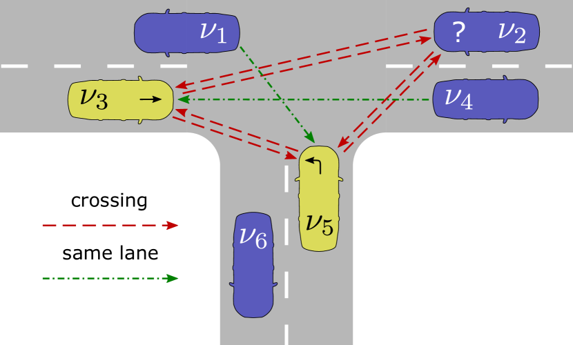
Figure 4: The graph-based input representation for mixed traffic modified from [3]. A CAV’s (yellow) turning intention is denoted by an arrow on its hood. Due to the unknown turning intention of the HDV $\nu_{2}$ (blue, denoted by ’?’), it shares edges with both CAVs, although only the conflict with $\nu_{5}$ is inevitable.

While CAVs share their desired route with the cooperative planner, the intention of human drivers is unknown. Therefore, the cooperative planner has to consider all possible conflicts with HDVs when coordinating CAVs. The graph-based scene representation inherently supports this by adding edges to an HDV for all conflicts that cannot be ruled out reliably. In the present work, we match the vehicle’s pose to lanes in a high definition (HD) map and enumerate viable continue paths. This assignment allows an angle between the vehicle heading the lane of up to $30\text{\,}\frac{\mathrm{\SIUnitSymbolDegree}}{}$ at the matched point. When crossing the intersection, a vehicle’s lane matches will thus reduce to the actual destination eventually, which then allows to plan the maneuver with less excess edges. The delay of this decision might be reduced further by employing a prediction algorithm, such as [33], which is out of scope for this work, though.

In addition to the semantic structure encoded in the graph, both vertices and edges are augmented by input feature sets. The vertex input features contain the vehicle’s longitudinal position along its lane, the driving speed, and measured acceleration. Additionally, a binary flag indicates whether the corresponding vehicle is a CAV to be coordinated or a HDV. The edge features are composed of a distance measure, heading-relative bearing, and the priority according to the map. The latter is required to enable the cooperative planner to correctly anticipate the behavior of HDVs that obey to the legacy priority rules.

The RL policy shall derive a joint action for all CAVs in the scene composed of longitudinal acceleration commands in continuous space for each vehicle. We employ the TD3 [34] actor-critic RL algorithm to train a GNN for the cooperative planning task. For conciseness, we present the actor network architecture in Fig. 5, while the critic’s architecture deviates only slightly on the output side. The input features for both vertices and edges are first encoded by MLPs with shared weights, respectively. For message passing in the GNN, we use modified relational graph convolutional network (RGCN) layers [35] as well as graph attention (GAT) layers [36]. The RGCN layers maintain independently learnable weight matrices per edge type and also incorporate the edge features in the vertex feature update. By introducing one intermediate GAT layer, the network may leverage the attention mechanism to focus on the most relevant interactions. A pure GAT network is not suited though, as the edge features are only used to compute the keys and queries, but not the values for the vertex feature update. Moreover, GAT does not consider the different edge types that are crucial for our graph-based representation.

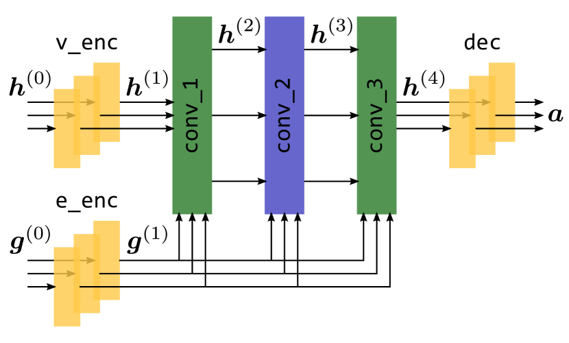
Figure 5: The GNN architecture of the actor network, as proposed in [3]. Vertex input features $\boldsymbol{h}^{(0)}$ and edge input features $\boldsymbol{g}^{(0)}$ are mapped to one joint action $\boldsymbol{a}$. The edge feature enhanced RGCN layers are depicted in green, the GAT layer in blue, and fully connected layers in yellow.

The resulting vertex features are finally mapped to a joint action by another MLP in the actor architecture. In contrast, the critic network aggregates the vertex feature vectors resulting from message passing to a single feature vector before decoding a Q-value estimate using an MLP. The graph-based scene representation and the GNN are implemented using the PyTorch Geometric API [37].

V-C Reward Function Engineering

Apart from a suited network architecture, RL requires a well-designed reward function to learn a reasonable policy. For solving the cooperative planning problem through RL, the reward function is defined as

$$R=\sum\limits_{k\in\mathcal{R}}w_{k}R_{k},$$ (8)

with $\mathcal{R}=\{\mathrm{velocity,\,idle,\,reluctance,\,proximity,\,collision}\}$ describing the set of reward components and $w_{k}$ the corresponding weights. The only positive reward component and thus the main driver for learning a nontrivial solution is the velocity reward, which is proportional to the average driving speed clipped to the lane speed limit. A trivial solution that consequently avoids any collision is to stop all vehicles in the scene. This is not a valid solution for cooperative maneuver planning and thus prevented through the idle penalty. In mixed traffic, the training tends to converge to a very conservative behavior, which manifests in all CAVs being stopped far away from the intersection to let HDVs pass [3]. This issue is addressed by the reluctance penalty, which is triggered for CAVs that drive very slowly without any lead vehicle. In order to facilitate learning of reasonable safety distances, the proximity reward penalizes situations in which CAVs get dangerously close. Ultimately, two vehicles colliding triggers the collision penalty and ends the training episode to avoid further positive rewards from being accumulated. The reward weights used throughout this study, at a policy frequency of $5\text{\,}\frac{\mathrm{Hz}}{}$, are given in Table II. Details on the definition and tuning of the various reward components can be found in [20, 3].

TABLE II: Reward weights

Reward	velocity	idle	reluctance	proximity	collision
Weight	0.06	0.02	0.02	0.2	1.0

V-D Derivation of Cooperative Maneuver

The maneuver representation introduced in Sec. III requires the cooperative maneuver to be specified over a sufficient horizon to facilitate local trajectory planning on the CAVs. This requirement for advance planning contrasts with the iterative nature of the RL policy, which requires immediate state feedback. In the present work, we build upon our approach from [26] to bridge this gap.

Based on the current traffic condition, a cooperative maneuver is derived by using a built-in simulator. After initializing the simulator based on the current state of the server-side EM, the RL policy is queried to predict the future evolution of the scene. We employ the same simulation environment that was used for training of the RL policy, based on Highway-env [38]. As depicted in Algorithm 1, the current simulator state is observed at $5\text{\,}\frac{\mathrm{Hz}}{}$ and passed to the RL policy $\pi$. While the simulated CAVs are moved according to the selected actions, the behavior of regular vehicles is predicted by the intelligent driver model (IDM, [39]), enhanced by the yielding logic from [21]. As the true destination of regular vehicles is not known to the cooperative planner, a worst-case route estimate is used. Thereby, all potential conflict points are considered while planning the cooperative maneuver.

Algorithm 1 Derive cooperative maneuver from initial server-side EM state according to [26].

1:Server-side EM, RL planning policy $\pi:\Omega\rightarrow A$.

2:Suggested maneuver for each vehicle $\mathcal{M}_{\nu}$.

3:$\mathrm{sim}\leftarrow\mathrm{initialize~{}simulator}$

4:for all $\nu\in\mathrm{EM}$ do

5:     $\mathrm{sim.addVehicle}(\boldsymbol{T}_{\nu},\,v_{\nu},\,\mathcal{D}_{\nu})$

6:end for

7:repeat

8:     $o\leftarrow\mathrm{sim.observe()}$

9:     $a\leftarrow\pi(o)$ # select next action

10:     $\mathrm{sim.step}(a)$

11:until all vehicles reached destination or timeout

12:for all $\nu\in\mathrm{EM}~{}\mathbf{if}~{}c_{\nu}~{}\mathrm{is~{}true}$ do

13:     $\mathcal{M}_{\nu}\leftarrow\mathrm{sim.getManeuver}(\nu)$

14:end for

15:return all $\mathcal{M}_{\nu}$

The simulation run is terminated when all vehicles have reached their destination, e.g., the desired side of the intersection, or optionally after a timeout. Typically, the overall planning response time remains below $1\text{\,}\frac{\mathrm{s}}{}$, however, it might occasionally exceed $2\text{\,}\frac{\mathrm{s}}{}$ in very crowded scenarios (more than ten vehicles present). In those cases, aborting the simulation by timeout is a viable measure to limit the response time. Because it is not ensured that every vehicle is guided to the end of the intersection area, cyclic replanning is required. In the current work, the cooperative maneuver is updated on a $2\text{\,}\frac{\mathrm{s}}{}$ period, as it was shown in [26] that even slight deviations in the predicted behavior can lead to maneuvers becoming infeasible. Especially with HDVs being present, cyclic replanning becomes imperative to ensure drivable maneuvers.

For each recorded simulated trajectory, waypoint candidates are created at the entry and exit of the intersection conflict area. The lower and upper bounds for traversing these waypoints is obtained from the simulation. Thereby, the entry waypoint determines the earliest possible time of entering the intersection. Analogously, the waypoint at the intersection entry specifies when the receiving CAV shall clear the conflict area at the latest.

VI Simulative Experiments

We integrated the proposed cooperative planning approaches into a new simulation and evaluation framework for fully automated and mixed traffic. The cooperative planners are evaluated and assessed against two baselines. Our primary baseline are non-cooperative (NC) CAVs that leverage shared perception data, but no routing information and adhere to priority rules. This baseline employs the same underlying trajectory planning as is used for the cooperative approaches. Thus, it constitutes a rather strong baseline, which facilitates a sharp evaluation of the cooperative aspect in isolation. In addition, we present the metrics for pure HDV traffic, which is simulated using a learned behavior model. As such, it resembles human driving behavior more closely and exhibits a human-typical agile behavior.

VI-A Simulation Setup

The simulation framework that we used for evaluation of the planning methods builds upon the DeepSIL simulator introduced in [40]. It is based on the ROS2 software distribution [41] and can simulate multiple HDVs as well as CAVs. The simulation has a base time step of $50\text{\,}\frac{\mathrm{ms}}{}$.

Human-driven vehicles are predicted using the approach in [40]. Every $50\text{\,}\frac{\mathrm{ms}}{}$, the multiple trajectory prediction network is evaluated on the current traffic environment. In each cycle, the most progressing, non-conflicting prediction is used to update the vehicle position and velocity. The prediction is converted into a longitudinal action and the internal vehicle simulation is stepped forward along the centerline of the route. The intersection handling was adapted to avoid collisions even in edge cases appearing in a large number of simulations. Also, an occlusion simulation was added, i.e. HDVs required to yield assume a blocked intersection and approach slowly until they have clear vision of the conflicting routes. The simulated HDVs do not know the routes of the other vehicles and therefore need to assume the most conflicting route.

Connected automated vehicles are simulated using a single-track model with friction and dead time, resembling one of our real-world CAVs. The inputs to this model are calculated by the trajectory planner from [42], which is part of this CAV’s software and therefore provides a realistic CAV behavior. Like HDVs, CAVs do not know the route of other vehicles, even of other CAVs, and assume the most conflicting route. However, the simulated CAVs do not need to approach the intersection slowly due to occlusion, because they receive the intersection EM as in [1].

VI-B Scenario Definition

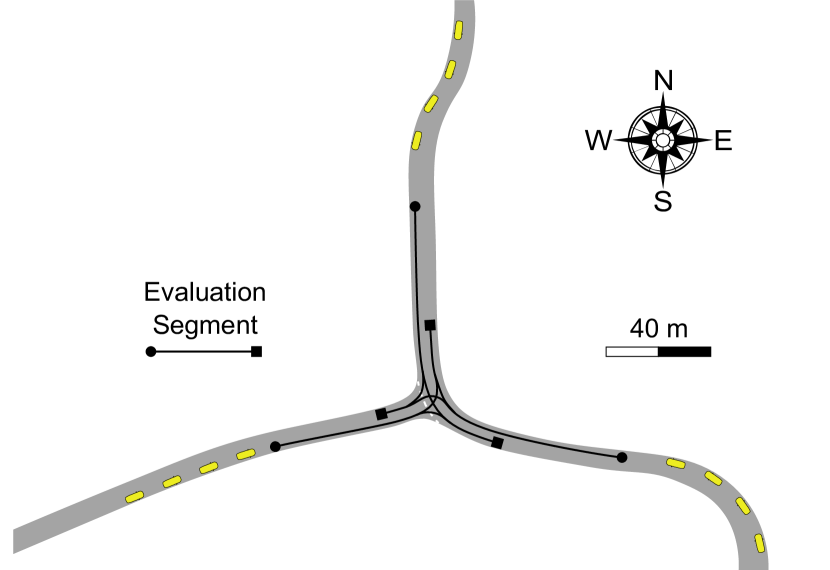
Figure 6: The initial positions of vehicles (yellow boxes) in the simulated scenarios. They are populated starting with the positions closest to the intersection. The evaluated trajectory segments are indicated by the black paths. The minor road approaches from the west.

We define all simulated scenarios at an exemplary intersection in Ulm-Lehr, Germany, as shown in Fig. 6, where also our pilot site (cf. Sec. VII-A) is located. It is a T-junction with a bending main road and a side road. The speed limit is $11.11\text{\,}\frac{\mathrm{m}}{\mathrm{s}}$ ($40\text{\,}\frac{\mathrm{km}}{\mathrm{h}}$) on the eastern and western part and $8.33\text{\,}\frac{\mathrm{m}}{\mathrm{s}}$ ($30\text{\,}\frac{\mathrm{km}}{\mathrm{h}}$) on the northern part.

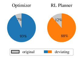
(a) Scenario crossing order

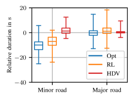
(b) Maneuver duration relative to NC baseline

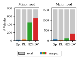
(c) Share of stopped vehicles

Figure 7: The simulative evaluation results in fully automated traffic for the optimization-based cooperative planner (Opt), the RL-based cooperative planner, and non-cooperative (NC) CAVs. HDV denotes pure HDV traffic.

Within this setting, we created a total set of 480 scenarios that serve as an initial configuration to the simulation. In each scenario, a number of vehicles is spawned at the locations shown in Fig. 6, where each vehicle has an initial speed of $8\text{\,}\frac{\mathrm{m}}{\mathrm{s}}$ and a specific route, i.e., turn direction. The first 280 scenarios are an enumeration of all combinations of source and target directions with up to two vehicles from each direction and in which there is at least one pair of conflicting vehicles. The remaining 200 scenarios are randomly sampled with up to four vehicles from each direction and a random route, limited to eight vehicles total due to computational constraints of the simulation.

The scenario set was simulated both in fully automated traffic and mixed traffic. When simulating mixed traffic, the vehicles are randomly divided into $50\text{\,}\frac{\mathrm{\char 37\relax}}{}$ HDVs and $50\text{\,}\frac{\mathrm{\char 37\relax}}{}$ CAVs, where for an odd number of vehicles, the last one is chosen randomly. Out of the 480 total scenarios, less than $3\text{\,}\frac{\mathrm{\char 37\relax}}{}$ of the simulations were not successful and resulted in a timeout or collision due to remaining issues in the simulation and trajectory planning frameworks (five scenarios in fully automated traffic, 14 scenarios in mixed traffic). Those scenarios were excluded from the evaluation in all maneuver planning configurations.

To ensure a fair comparison, all trajectories have been clipped to common evaluation intervals, as illustrated in Fig. 6. The following evaluations refer to trajectory segments that begin $60\text{\,}\frac{\mathrm{m}}{}$ in front of the intersection entry ($\bullet$ in Fig. 6) and end $15\text{\,}\frac{\mathrm{m}}{}$ behind the intersection ($\blacksquare$ in Fig 6). These intervals cover the relevant part of the intersection approach during which the CAVs synchronize onto their assigned slot for crossing the intersection.

VI-C Quantitative Results

Figure 7 depicts the results in fully automated traffic. Both planners are able to realize cooperative maneuvers in the vast majority of scenarios, as can be seen from Fig. LABEL:sub@sfig:all_cav_deviating. A scenario run is considered cooperative if the vehicle crossing order deviates from the baseline crossing order. For comparability, the following analyses are performed over all scenarios in which at least one cooperative planner suggested a deviating crossing order. In the cooperative scenarios, the traffic flow especially on the minor road is improved significantly, while the optimization-based planner provides an additional benefit over the RL-based one. Figure LABEL:sub@sfig:all_cav_relative_duration_road_type depicts the distribution of the duration required by the vehicles to complete the maneuver relative to non-cooperative CAVs. Almost all vehicles on the minor road benefit of a reduced delay due to interaction. Some vehicles on the major road take slightly longer to complete the maneuver in the cooperative case. This is expected since the vehicles on the major road waive their unconditional right of way when taking part in cooperative maneuvers. Overall, the cooperation leads to a reduction in median duration, which becomes even more pronounced when comparing to pure HDV traffic.

Having a vehicle stop is particularly disadvantageous in terms of both energy efficiency and passenger comfort. As can be observed in Fig. LABEL:sub@sfig:all_cav_stopped_vehicles_road_type, both cooperative planners eliminate most of the stops required on the minor road when driving according to priority rules. Notably, the share of stopped vehicles on the major road does not increase but even decrease slightly, which can mainly be attributed to left-turning vehicles yielding to oncoming traffic. Pure HDV traffic exhibits much more stops because they cannot rely on shared perception data and thus have to approach the intersection more carefully.

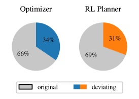
(a) Scenario crossing order

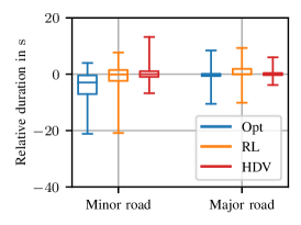
(b) Maneuver duration relative to NC baseline

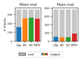
(c) Share of stopped vehicles

Figure 8: The simulative evaluation results in mixed traffic under $50\text{\,}\frac{\mathrm{\char 37\relax}}{}$ automation level for the optimization-based cooperative planner (Opt), the RL-based cooperative planner, and non-cooperative (NC) CAVs. HDV denotes pure HDV traffic.

The cooperative planning approaches also raise improvement potential in mixed traffic efficiency, as illustrated by Fig. 8. Both the optimization-based planner and the RL planner suggest a cooperative maneuver in significantly fewer cases compared to fully automated traffic. It is worth noting that a $50\text{\,}\frac{\mathrm{\char 37\relax}}{}$ share of HDVs renders many cooperative maneuvers infeasible because the priority relations towards HDVs have to be retained. The following metrics again refer to all scenarios in which at least one cooperative planner suggested a deviating crossing order.

Figure LABEL:sub@sfig:mixed_relative_duration_road_type indicates that still many vehicles on the minor road benefit of a reduced delay due to the cooperative maneuver. It is important to note that the simulation setup only considers the evaluation of the initial vehicle configuration, but not continuous traffic. Unlike in real traffic, the vehicles on the minor road will be able to cross the intersection fluently after the prioritized traffic has left the intersection. This circumstance leads to a favoritism of the baseline maneuvers, which might have taken much longer in real continuous traffic. Nonetheless, a reduction of stops can be observed in Fig. LABEL:sub@sfig:mixed_stopped_vehicles_road_type also for mixed traffic. Here, the optimization-based planner clearly outperforms the RL-based planner in terms of stops on the minor road. This can most likely be attributed to the training of the RL being performed in continuous traffic to facilitate learning of a robust policy. In the case of evaluating single scenarios, the learned efficiency estimation of the RL model might not be accurate.

VII Real-World Experiments

To support our simulative results, we also conducted test drives in real-world traffic. Although a similar quantitative evaluation as in simulation is not possible, this shows that our cooperative maneuver planning system can be successfully deployed to a real-world setup of connected intelligent infrastructure and CAVs.

VII-A Pilot Site Ulm-Lehr

The real-world experiments were conducted at a pilot site for connected automated driving in Ulm-Lehr, Germany [1]. The intersection is equipped with multiple sensor processing units, each consisting of cameras, radar and lidar sensors as well as a computer for object detection. An edge server resides in the same 5G cellular network cell and a fusion and tracking module [43] combines all object detections into the infrastructure EM, which is provided to the connected vehicles and the cooperative planning modules. The latter also run on the edge server. We employed three CAVs, of which one used the trajectory planning from [42] as mentioned before, and the other two implemented the concept from [44].

The scenario that was investigated in real-world experiments comprises the three CAVs approaching the intersection from each of its accesses, as depicted in Fig. 1. Vehicle $\nu_{3}$ approaches the intersection on the main road coming from north and following the road. According to ordinary priority rules, this vehicle has the right of way. Vehicle $\nu_{1}$ starts at the other main road access (east) and intents to turn left at the intersection. This vehicle vehicle would have to yield to the oncoming traffic but not to any vehicle coming from the side road. With vehicle $\nu_{2}$ approaching the intersection from the west on the minor road, it would have to yield to all cross traffic. As it intents to turn right at the intersection, there is no conflict with $\nu_{1}$ but only with $\nu_{3}$. Figure 1 illustrates a typical cooperative maneuver. If vehicle $\nu_{3}$ waives its right of way and possibly slows down while approaching, it allows both other CAVs to cross the intersection virtually simultaneously. Depending on the timing, vehicles $\nu_{1}$ and $\nu_{2}$ can simply traverse the intersection unimpeded. Ideally, vehicle $\nu_{3}$ should not be required to stop, but slow down smoothly and accelerate again once the intersection is cleared.

VII-B Evaluation in Real-World

To obtain a reliable quantitative evaluation in real traffic, the initial scenario depicted in Fig. 1 was driven numerous times. Thereof, five baseline runs have been performed by driving according to priority rules, twelve runs under the command of the optimization-based planner, and 20 runs employing the RL planner. The cooperative maneuvers have been planned reactively with respect to surrounding traffic. One of the evaluation runs using the RL planner was recorded on video for demonstration purposes and is available at [45]. The vehicles’ trajectories have been recorded and clipped to the common evaluation segment, which was also used for the simulative evaluation. Because all experiments have been conducted in real traffic at a public intersection, the initial conditions are not ensured to match perfectly. While the safety drivers guided the test vehicles carefully to the engagement point, minor deviations in timing and initial speed remain. During all maneuver runs that are contained in the evaluation, the automated driving system was successfully engaged for at least the whole evaluation segment.

One of the most expressive metrics for traffic efficiency at intersections is the delay induced by interaction with other vehicles. In the present work, we consider the maneuver duration, i.e., the time it takes for a vehicle to cross the evaluation segment, relative to the median baseline duration. Therefore, the median bars of the baseline distribution in the boxplot in Fig. 9 are exactly at a duration of $0\text{\,}\frac{\mathrm{s}}{}$. The outlier of vehicle $\nu_{1}$ at around $-3.5\text{\,}\frac{\mathrm{s}}{}$ can be explained by a deviation in initial timing. In this run, the vehicle did not have to stop and its driving speed remained above $3\text{\,}\frac{\mathrm{m}}{\mathrm{s}}$. It can be observed that both cooperative planning approaches yield a significant reduction in maneuver duration for the vehicles $\nu_{1}$ and $\nu_{2}$, which cross the intersection simultaneously in the cooperative maneuver. While the time gain for each of these vehicles is roughly $7\text{\,}\frac{\mathrm{s}}{}$, the vehicle $\nu_{3}$ on the major road rarely looses more than $2\text{\,}\frac{\mathrm{s}}{}$ during the approach and traversal of the intersection. It can be concluded that both cooperative planners are able to identify traffic scenes in which the ordinary priority rules yield sub-optimal flow and propose a more efficient maneuver.

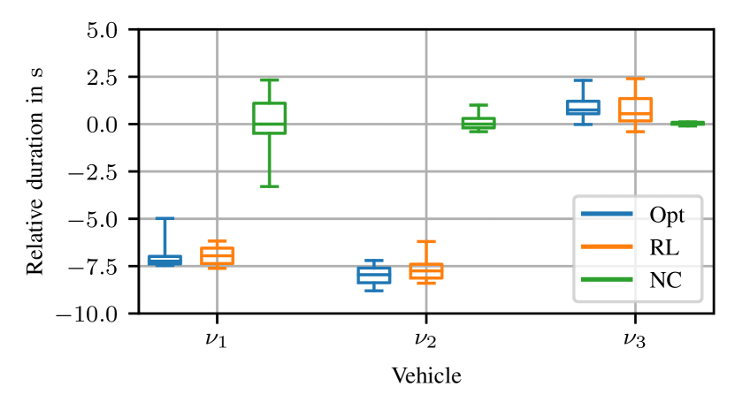
Figure 9: The maneuver duration for each involved CAV relative to the median baseline duration.

In addition, we present the average speed distribution over all vehicles in Fig. 10. Both cooperative planners yield a mean driving speed of around $7.5\text{\,}\frac{\mathrm{m}}{\mathrm{s}}$ ($27\text{\,}\frac{\mathrm{km}}{\mathrm{h}}$) over the evaluated trajectory segment. Considering the lane curvature on the confined intersection space, this indicates a swift intersection traversal without any stops. In contrast, when driving according to priority rules, the average speed remains below $5\text{\,}\frac{\mathrm{m}}{\mathrm{s}}$. Undoubtedly, the yielding behavior of the vehicles $\nu_{1}$ and $\nu_{2}$ might lead to stops in this case, which causes a decrease in driving speed and efficiency.

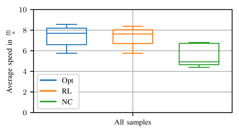
Figure 10: The average driving speed over all CAVs when coordinated by one of the cooperative planners compared to baseline driving.

VIII Conclusion

In this paper, an optimization-based and an RL-based approach for cooperative maneuver planning in mixed traffic at urban intersections have been compared. The proposed approaches have been evaluated in simulation and in real-world experiments using three prototype CAVs. Compared to HDVs adhering to priority rules and non-cooperative CAVs, the cooperative maneuvers lead to improved traffic efficiency. In simulated fully automated traffic, a significant reduction of delay due to interaction and of the share of stopped vehicles has been shown. In mixed traffic with $50\text{\,}\frac{\mathrm{\char 37\relax}}{}$ CAV penetration, the proposed planners still found a viable cooperative maneuver in about one third of the scenarios. Both cooperative planners demonstrated their real-world applicability in public traffic and yielded a significant reduction in delay due to interaction. Future work will include the evaluation of further cooperative use cases in urban traffic involving human-driven CVs and vulnerable road users.

Marvin Klimke (marvin.klimke@de.bosch.com) earned his M.Sc. degree in Electrical Engineering with a major focus on Computer Engineering in 2021 from RWTH Aachen University. He is a PhD student with the Department of Corporate Research, Robert Bosch GmbH, Stuttgart, 70049, Germany, and the Institute of Measurement, Control, and Microtechnology, Ulm University, Ulm, 89081, Germany. His research interests include connected automated driving as well as behavior planning for automated driving by employing machine learning.

Max Bastian Mertens (max.mertens@uni-ulm.de) earned his M.Sc. degree in Communications and Computer Engineering at Ulm University in 2020. He is a researcher at the Institute of Measurement, Control, and Microtechnology, Ulm University, Ulm, 89081, Germany. His research interests include trajectory and cooperative maneuver planning as well as scene prediction in mixed traffic.

Benjamin Völz (benjamin.voelz@de.bosch.com) earned his diploma degree from the Faculty of Electrical and Computer Engineering, Dresden University of Technology, and his Ph.D. degree from the Department of Mechanical and Process Engineering, ETH Zurich. He is a research engineer at Robert Bosch, Stuttgart, 70049, Germany, focusing on planning for connected urban automated driving. His research interests include scene analysis, prediction, decision making, and planning for automated vehicles.

Michael Buchholz (michael.buchholz@uni-ulm.de) received his Diploma degree in Electrical Engineering and Information Technology as well as his Ph.D. from the faculty of Electrical Engineering and Information Technology at University of Karlsruhe (TH)/Karlsruhe Institute of Technology, Germany. He is a research group leader and lecturer at the Institute of Measurement, Control, and Microtechnology, Ulm University, Ulm, 89081, Germany, where he earned his “Habilitation” (post-doctoral lecturing qualification) for Automation Technology in 2022. His research interests comprise connected automated driving, electric mobility, modelling and control of mechatronic systems, and system identification.

References

- [1] M. Buchholz, J. Müller, M. Herrmann, J. Strohbeck, B. Völz, M. Maier, J. Paczia, O. Stein, H. Rehborn, and R.-W. Henn, “Handling Occlusions in Automated Driving Using a Multiaccess Edge Computing Server-Based Environment Model From Infrastructure Sensors,” IEEE Intell. Transp. Syst. Magazine, vol. 14, no. 3, pp. 106–120, 2022.
- [2] M. B. Mertens, J. Müller, and M. Buchholz, “Cooperative Maneuver Planning for Mixed Traffic at Unsignalized Intersections Using Probabilistic Predictions,” in 2022 IEEE Intell. Veh. Symp. (IV), 2022, pp. 1174–1180.
- [3] M. Klimke, B. Völz, and M. Buchholz, “Automatic Intersection Management in Mixed Traffic Using Reinforcement Learning and Graph Neural Networks,” in 2023 IEEE Intell. Veh. Symp. (IV), 2023, pp. 1–8.
- [4] M. B. Mertens, J. Müller, R. Dehler, M. Klimke, M. Maier, S. Gherekhloo, B. Völz, R.-W. Henn, and M. Buchholz, “An Extended Maneuver Coordination Protocol with Support for Urban Scenarios and Mixed Traffic,” in 2021 IEEE Veh. Netw. Conf. (VNC), 2021, pp. 32–35.
- [5] Z. Zhong, M. Nejad, and E. E. Lee, “Autonomous and Semiautonomous Intersection Management: A Survey,” IEEE Intell. Transp. Syst. Magazine, vol. 13, no. 2, pp. 53–70, 2021.
- [6] P. R. Lowrie, “The Sydney coordinated adaptive traffic system - principles, methodology, algorithms,” 1982. [Online]. Available: https://trid.trb.org/view.aspx?id=1188851
- [7] X.-H. Yu and A. Stubberud, “Markovian decision control for traffic signal systems,” in Proc. of the 36th IEEE Conf. on Decision and Control, vol. 5, 1997, pp. 4782–4787 vol.5.
- [8] L. Li and F.-Y. Wang, “Cooperative Driving at Blind Crossings Using Intervehicle Communication,” IEEE Transactions on Veh. Technol., vol. 55, no. 6, pp. 1712–1724, 2006.
- [9] J. Wu, A. Abbas-Turki, and A. El Moudni, “Cooperative driving: an ant colony system for autonomous intersection management,” Applied Intelligence, vol. 37, no. 2, pp. 207–222, 2012.
- [10] K. Dresner and P. Stone, “Multiagent traffic management: a reservation-based intersection control mechanism,” in Proc. of the Third Int. Joint Conf. on Autonomous Agents and Multiagent Syst., 2004. AAMAS 2004., 2004, pp. 530–537.
- [11] C. Wuthishuwong and A. Traechtler, “Vehicle to infrastructure based safe trajectory planning for Autonomous Intersection Management,” in 2013 13th Int. Conf. on ITS Telecommunications (ITST), 2013, pp. 175–180.
- [12] M. R. Hafner, D. Cunningham, L. Caminiti, and D. Del Vecchio, “Cooperative Collision Avoidance at Intersections: Algorithms and Experiments,” IEEE Transactions on Intell. Transp. Syst., vol. 14, no. 3, pp. 1162–1175, 2013.
- [13] F. Yan, M. Dridi, and A. El Moudni, “Autonomous vehicle sequencing algorithm at isolated intersections,” in 2009 12th Int. IEEE Conf. on Intell. Transp. Syst., 2009, pp. 1–6.
- [14] M. Ahmane, A. Abbas-Turki, F. Perronnet, J. Wu, A. E. Moudni, J. Buisson, and R. Zeo, “Modeling and controlling an isolated urban intersection based on cooperative vehicles,” Transp. Research Part C: Emerging Technologies, vol. 28, pp. 44–62, 2013.
- [15] R. Hult, M. Zanon, S. Gras, and P. Falcone, “An MIQP-based heuristic for Optimal Coordination of Vehicles at Intersections,” in 2018 IEEE Conf. on Decision and Control (CDC), 2018, pp. 2783–2790.
- [16] K. Yang, S. I. Guler, and M. Menendez, “Isolated intersection control for various levels of vehicle technology: Conventional, connected, and automated vehicles,” Transp. Research Part C: Emerging Technologies, vol. 72, pp. 109–129, 2016.
- [17] K. Kurzer, C. Zhou, and J. Marius Zöllner, “Decentralized Cooperative Planning for Automated Vehicles with Hierarchical Monte Carlo Tree Search,” in 2018 IEEE Intell. Veh. Symp. (IV), 2018, pp. 529–536.
- [18] J. Cui, H. Qiu, D. Chen, P. Stone, and Y. Zhu, “Coopernaut: End-to-End Driving with Cooperative Perception for Networked Vehicles,” in IEEE/CVF Conf. on Computer Vision and Pattern Recognition (CVPR), 2022, pp. 17 252–17 262.
- [19] Y. Wu, H. Chen, and F. Zhu, “DCL-AIM: Decentralized Coordination Learning of Autonomous Intersection Management for Connected and Automated Vehicles,” Transp. Research Part C: Emerging Technologies, vol. 103, pp. 246–260, 2019.
- [20] M. Klimke, B. Völz, and M. Buchholz, “Cooperative Behavior Planning for Automated Driving Using Graph Neural Networks,” in 2022 IEEE Intell. Veh. Symp. (IV), 2022, pp. 167–174.
- [21] M. Klimke, J. Gerigk, B. Völz, and M. Buchholz, “An Enhanced Graph Representation for Machine Learning Based Automatic Intersection Management,” in 2022 IEEE Int. Conf. on Intell. Transp. Syst. (ITSC), 2022, pp. 523–530.
- [22] K. Dresner and P. Stone, “Sharing the Road: Autonomous Vehicles Meet Human Drivers,” in IJCAI, 2007.
- [23] L. C. Bento, R. Parafita, S. Santos, and U. Nunes, “Intelligent traffic management at intersections: Legacy mode for vehicles not equipped with V2V and V2I communications,” in 16th Int. IEEE Conf. on Intell. Transp. Syst. (ITSC 2013), 2013, pp. 726–731.
- [24] D. Quang Tran and S.-H. Bae, “Proximal Policy Optimization Through a Deep Reinforcement Learning Framework for Multiple Autonomous Vehicles at a Non-Signalized Intersection,” Applied Sciences, vol. 10, no. 16, p. 5722, 2020.
- [25] Z. Guo, Y. Wu, L. Wang, and J. Zhang, “Coordination for Connected and Automated Vehicles At Non-Signalized Intersections: A Value Decomposition-Based Multiagent Deep Reinforcement Learning Approach,” IEEE Transactions on Veh. Technol., pp. 1–11, 2022.
- [26] M. Klimke, B. Völz, and M. Buchholz, “Integration of Reinforcement Learning Based Behavior Planning With Sampling Based Motion Planning for Automated Driving,” in 2023 IEEE Intell. Veh. Symp. (IV), 2023, pp. 1–8.
- [27] ETSI EN 302 637-2, “Intelligent Transport Systems (ITS); Vehicular Communications; Basic Set of Applications; Part 2: Specification of Cooperative Awareness Basic Service,” 2014, final draft V1.3.1.
- [28] ETSI TR 103 562, “Intelligent Transport Systems (ITS); Vehicular Communications; Basic Set of Applications; Analysis of the Collective Perception Service (CPS); Release 2,” 2019, v2.1.1.
- [29] M. B. Mertens, J. Ruof, J. Strohbeck, and M. Buchholz, “Fast Long-Term Multi-Scenario Prediction for Maneuver Planning at Unsignalized Intersections,” in Accepted for: 2024 American Control Conf. (ACC), 2024, preprint available: http://arxiv.org/abs/2401.14879.
- [30] J. Schulman, F. Wolski, P. Dhariwal, A. Radford, and O. Klimov, “Proximal Policy Optimization Algorithms,” 2017, arXiv:1707.06347. [Online]. Available: http://arxiv.org/abs/1707.06347
- [31] J. Bock, R. Krajewski, T. Moers, S. Runde, L. Vater, and L. Eckstein, “The inD Dataset: A Drone Dataset of Naturalistic Road User Trajectories at German Intersections,” in 2020 IEEE Intell. Veh. Symp. (IV), 2020, pp. 1929–1934.
- [32] S. Gronauer and K. Diepold, “Multi-Agent Deep Reinforcement Learning: A Survey,” Artificial Intelligence Review, 2021.
- [33] J. Strohbeck, V. Belagiannis, J. Müller, M. Schreiber, M. Herrmann, D. Wolf, and M. Buchholz, “Multiple Trajectory Prediction with Deep Temporal and Spatial Convolutional Neural Networks,” in 2020 IEEE/RSJ Int. Conf. on Intell. Robots and Syst. (IROS), 2020, pp. 1992–1998.
- [34] S. Fujimoto, H. van Hoof, and D. Meger, “Addressing Function Approximation Error in Actor-Critic Methods,” in Proc. of the 35th Int. Conf. on Machine Learning, ser. Proc. of Machine Learning Research, J. Dy and A. Krause, Eds., vol. 80, 2018, pp. 1587–1596.
- [35] M. Schlichtkrull, T. N. Kipf, P. Bloem, R. van den Berg, I. Titov, and M. Welling, “Modeling Relational Data with Graph Convolutional Networks,” in The Semantic Web, A. Gangemi, R. Navigli, M.-E. Vidal, P. Hitzler, R. Troncy, L. Hollink, A. Tordai, and M. Alam, Eds. Springer Int. Publishing, 2018, vol. 10843, pp. 593–607.
- [36] P. Veličković, G. Cucurull, A. Casanova, A. Romero, P. Liò, and Y. Bengio, “Graph Attention Networks,” in Int. Conf. on Learning Representations, 2018.
- [37] M. Fey and J. E. Lenssen, “Fast Graph Representation Learning with PyTorch Geometric,” 2019. [Online]. Available: https://github.com/pyg-team/pytorch_geometric
- [38] E. Leurent, “An Environment for Autonomous Driving Decision-Making,” 2018. [Online]. Available: https://github.com/eleurent/highway-env
- [39] M. Treiber, A. Hennecke, and D. Helbing, “Congested Traffic States in Empirical Observations and Microscopic Simulations,” Physical Review E, vol. 62, no. 2, pp. 1805–1824, 2000.
- [40] J. Strohbeck, J. Müller, A. Holzbock, and M. Buchholz, “DeepSIL: A Software-in-the-Loop Framework for Evaluating Motion Planning Schemes Using Multiple Trajectory Prediction Networks,” in 2021 IEEE/RSJ Int. Conf. on Intell. Robots and Syst. (IROS). IEEE Press, 2021, pp. 7075–7081.
- [41] S. Macenski, T. Foote, B. Gerkey, C. Lalancette, and W. Woodall, “Robot operating system 2: Design, architecture, and uses in the wild,” Science Robotics, vol. 7, no. 66, 2022.
- [42] J. Ruof, M. B. Mertens, M. Buchholz, and K. Dietmayer, “Real-Time Spatial Trajectory Planning for Urban Environments Using Dynamic Optimization,” in 2023 IEEE Intell. Veh. Symp. (IV), 2023, pp. 1–7.
- [43] M. Herrmann, J. Müller, J. Strohbeck, and M. Buchholz, “Environment Modeling Based on Generic Infrastructure Sensor Interfaces Using a Centralized Labeled-Multi-Bernoulli Filter,” in 2019 IEEE Intell. Transp. Syst. Conf. (ITSC), 2019, pp. 2414–2420.
- [44] B. Völz, A. Stamm, M. Maier, R.-W. Henn, R. Siegwart, and J. Nieto, “Towards Infrastructure-Supported Planning for Urban Automated Driving,” in Robotics: Science and Systems (RSS), Workshop on Scene and Situation Understanding for Autonomous Driving, 2019.
- [45] Robert Bosch GmbH and Institute of Measurement, Control, and Microtechnology, “LUKAS Project: Overview and Use Case Results,” doi: 10.18725/OPARU-51253.