Inferring system parameters from the bursts of the accretion-powered pulsar IGR J17498–2921

Abstract

Thermonuclear (type-I) bursts exhibit properties that depend both on the local surface conditions of the neutron stars on which they ignite, as well as the physical parameters of the host binary system. However, constraining the system parameters requires a comprehensive method to compare the observed bursts to simulations. We have further developed the beansp code for this purpose and analysed the bursts observed from IGR J17498$-$2921, a 401-Hz accretion-powered pulsar, discovered during it’s 2011 outburst. We find good agreement with a model having H-deficient fuel with $X=0.15\pm 0.4$, and CNO metallicity about a tenth of the solar value. The model has the system at a distance of $5.7^{+0.6}_{-0.5}$ kpc, with a massive ($\approx 2\ M_{\odot}$) neutron star and a likely inclination of $60^{\circ}$. We also re-analysed the data from the 2002 outburst of the accretion-powered millisecond pulsar SAX J1808.4$-$3658. For that system we find a substantially closer distance than previously inferred, at $2.7\pm 0.3$ kpc, likely driven by a larger degree of burst emission anisotropy. The other system parameters are largely consistent with the previous analysis. We briefly discuss the implications for the evolution of these two systems.

1 Introduction

Accretion-powered millisecond pulsars (AMSPs) are a high observational priority due to their rarity (only 20 are known; Di Salvo & Sanna, 2022) and their significance as the evolutionary precursors of “recycled” millisecond radio pulsars (e.g. Alpar et al., 1982). This link has been confirmed in spectacular fashion with the discovery in recent years of “transitional” pulsars which switch between rotation-powered (radio) and accretion-powered (X-ray) pulsar phases, including the M28 transient IGR 18245$-$2452, which is also known as PSR J1824$-$2452I (e.g. Linares et al., 2014). Millisecond radio pulsars (MSRPs) are thought to go through an AMSP stage, but present AMSPs have a distinctly different orbital period distribution compared to present-day MSRPs (e.g. Tauris et al., 2012; Papitto et al., 2014).

AMSPs are typically discovered when they undergo a transient outburst, during which the accretion rate (and hence the X-ray luminosity) increases by several orders of magnitude in $\approx 1$ d (e.g. Goodwin et al., 2020). This behaviour is also observed in the broader class of low-mass X-ray binaries, but the peak accretion rates reached by the AMSPs is typically lower.

Thermonuclear (type-I) bursts have been observed during the outbursts of some AMSPs, and are of particular interest due to their utility for constraining the properties of the host systems (e.g. Galloway & Keek, 2021). The bursts from AMSPs typically exhibit burst oscillations at the pulse (spin) frequency Patruno & Watts (2012). They tend to be of short duration, indicative of H-deficient fuel, and with a high incidence of photospheric radius-expansion. These properties are generally associated with accretion at low (few % Eddington) rates, as inferred from the persistent X-ray emission.

SAX J1808.4$-$3658 was the first AMSP discovered in ’t Zand et al. (1998); Wijnands & van der Klis (1998); Chakrabarty & Morgan (1998), and has been observed in outburst a total of 11 times (e.g. Illiano et al., 2023). The bursts from SAX J1808.4$-$3658 are perhaps the best-studied of all. First discovered with the BeppoSAX/WFC in ’t Zand et al. (1998), subsequent events have been observed by several missions, including simultaneously with Chandra & RXTE in ’t Zand et al. (2013) demonstrating the boost in persistent flux associated with bursts Worpel et al. (2013, 2015). With NICER a complex 2-stage flux evolution in the rise has been observed, implying compositional interactions with the radius-expansion phenomenon (Bult et al. 2019; see also Galloway et al. 2006). The 2019 outburst, which was detected unusually early thanks to coordinated optical and X-ray monitoring Goodwin et al. (2020), revealed with NICER and NuSTAR unusually weak bursts, attributed to H-ignition rather than the usual He Casten et al. (2023).

Several attempts have been made to match the bursts from SAX J1808.4$-$3658 to 1-D ignition models, beginning with Galloway & Cumming (2006). Johnston et al. (2018) generated plausible sequences of bursts for the same outburst with the kepler code. Goodwin et al. (2019, hereafter G19) developed a Bayesian framework (beansp) and constrained the fuel composition, as well as the system parameters, demonstrating that the mass donor was H-deficient. These constraints also have consequences for the evolution of the system Goodwin & Woods (2020).

In order to further develop the capabilities of the beansp code, in this work we applied it to the 2011 outburst of IGR J17498$-$2921. This pulsar towards the Galactic centre ($l=0.16$, $b=-1.00$) was discovered by INTEGRAL when it went into outburst in 2011 August Papitto et al. (2011), and was active for $\approx 40$ d subsequently. The source consists of a neutron star rotating with a spin frequency of 401 Hz, and a binary companion orbiting once every 3.8 hr. Thermonuclear bursts were detected during the outburst, first by INTEGRAL/JEM-X Ferrigno et al. (2011), as well as subsequently by RXTE/PCA and Swift. The bursts were short duration (6–10 s) and were consistent with recurrence times in the range 16–18 hr. As with other AMSPs, the bursts exhibited burst oscillations at a frequency consistent with the persistent pulsations, with only one having evidence for photospheric radius expansion. The implied distance (neglecting any burst anisotropy) is in the range 6.6–8.1 kpc. The source was detected once again in outburst in 2023 April Grebenev et al. (2023); Sanna et al. (2023) but no bursts have been reported.

In this paper we describe our efforts to constrain the system parameters for IGR J17498$-$2921 via comparison of the observed bursts with a numerical ignition model. In §2 we describe the comparison approach, via the beansp code. In §3 we describe the observational data used for the analysis, and give more detail about how the the Markov-Chain Monte Carlo (MCMC) algorithm is used to constrain the system parameters. In §4 we describe the results of the MCMC runs, and the corresponding constraints derived on the target systems. Finally, in §5 we discuss the results and the next steps.

2 Methods

We adopted the same approach as G19 for matching bursts to numerical models, but have made substantial improvements to the beansp code base, which is now available via the Python Package Index (PYPI).

The burst matching algorithm relies on the ignition code of Cumming & Bildsten (2000), which has now been improved and updated and is available as pySettle also via PYPI. This code now gives correct values for the $\alpha$-parameter, i.e. the ratio of the persistent luminosity to the burst luminosity, in the observer frame for consistency with the burst recurrence time and energy. The 0.65 correction factor adopted by G19 for the burst recurrence time $\Delta t$ and fluence $E_{b}$ has now been removed from the pySettle code, and incorporated instead as a correction function within beansp. Examination of the code suggests that previously the factor was applied only to the recurrence time, and the fluence was unchanged. We provide the function corr_goodwin19 to replicate the runs from this and the previous paper, but the user can also provide their own.

beansp uses the emcee implementation of the affine-invariant Markov-Chain Monte-Carlo (MCMC) sampler Foreman-Mackey et al. (2013). Earlier versions of the code relied on conversion of model-predicted burst parameters to observational equivalents, via three ratios from which the physical parameters could be determined. Since the original version of the code used a fixed mass and radius, and the option to vary those parameters was introduced later, we cannot be confident that the conversion of the ratios to physical parameters correctly incorporated varying mass and radius. The present version supplants this approach and replaces the three ratios with explicit physical parameters distance $d$, and the emission anisotropies of the burst and persistent flux, $\xi_{b}$ and $\xi_{p}$, respectively. The anisotropies are defined in the same sense as for He & Keek (2016), i.e. the flux measured by an observer $F_{b,p}$ is related to the total luminosity $L_{b,p}$ by

$$F_{b,p}=\frac{L_{b,p}}{4\pi d^{2}\xi_{b,p}}$$ (1)

so that (for example) $\xi_{b,p}>1$ indicates that the emission is beamed preferentially out of the observer’s line of sight, so the observed flux is lower than would be expected for isotropic emission.

Other modifications to the code used in this work include corrections to the conversion between flux and accretion rate (parameterised in units of the Eddington rate, $1.75\times 10^{-9}[1.7/(1+X)]\ M_{\odot}\,{\rm yr^{-1}}$ where $X$ is the hydrogen mass fraction) for pySettle. The user can now choose different options for integrating the persistent flux between bursts (to calculate the average accretion rate for the purposes of predicting the burst properties). Previously the code would interpolate linearly between flux measurements; this approach causes problems for the simulation algorithm due to local maxima (which may or may not be real) in the flux history. The user can instead choose to approximate the flux history with a B-spline representation (splrep in scipy; Virtanen et al., 2020), with user-defined smoothing factor.

The flexibility of the beansp code has been substantially improved, facilitating exploration of the parameter space. The user can opt to omit the comparison of the measured $\alpha$ values, and only compare the burst times and fluences. This approach might be preferred for cases where the precise burst count through observing gaps cannot be maintained, so that the precise recurrence time is unknown. Additionally, there is the question of how independent the $\alpha$-values are, since they are calculated from the fluences combined with the recurrence time and the persistent fluxes. For those reasons, the runs reported in this paper were all performed with alpha=False. The user can further also omit the fluences from the comparison if an initial match purely on the burst times is desired. Bursts for which the fluence cannot be measured can still be included in the likelihood calculation on the basis of their start time alone. Previously the likelihood calculation included multiplicative factors $f_{i}$ (see their equation 11) to account for possible underestimation of the variance. The present version can be run with or without these additional factors.

3 Observations & Simulations

As a primary source we used burst analyses from the Multi-INstrument Burst ARchive (MINBAR; Galloway et al., 2020), which includes analyses of all bursts observed with the RXTE Proportional Counter Array (PCA), BeppoSAX Wide-Field Camera (WFC) and the INTEGRAL Joint European Monitor for X-rays (JEM-X) through to 2012 January. Where necessary, we augmented these data with additional burst and persistent flux measurements observed with instruments not contributing to that sample.

The burst measurements comprised the start time, typically measured as the time that the burst flux first exceeded 25% of the maximum reached during the burst. The burst fluence $E_{b}$ is calculated from time-resolved spectroscopy covering the burst. The $\alpha$-value, where used, is calculated as

$$\alpha_{i}=\frac{F_{p,i}c_{\rm bol}\Delta t}{E_{b,i}}$$ (2)

where $F_{p,i}$ is the average persistent flux over the interval from the previous burst, $\Delta t$, $E_{b,i}$ is the fluence of burst $i$, and $c_{\rm bol}$ is the bolometric correction required for the flux, which is usually measured in a restricted energy band (3–25 keV for the instruments contributing to MINBAR).

In order to verify the new version of the code against the old, we re-analysed the bursts from the 2002 outburst of SAX J1808.4$-$3658 as well as the 2011 outburst of IGR J17498$-$2921, as described below.

3.1 SAX J1808.4–3658

We adopted the same data used by G19, obtained from RXTE/PCA observations of the 2002 outburst and analysed as part of the MINBAR sample. The data comprises four bursts and persistent flux measurements with RXTE/PCA covering the interval 2002 October 15–-23 (MJD 52562–52570; Table 1). As the persistent fluxes are measured from spectral fits in the 3–25 keV range, we adopted a constant bolometric correction of 2.21 over the course of the outburst. We used the spline approximation to integrate the persistent flux between bursts for the purposes of burst simulation, with smoothing factor 0.02.

3.2 IGR J17498–2921

We adopted the persistent fluxes in the 0.1–300 keV range estimated by Falanga et al. (2012), covering the outburst interval of 2011 August 12–September 21 (MJD 55785–55825; Fig. 1). As the energy band is already sufficiently wide we take those fluxes as bolometric, and so do not require an additional correction. Those authors also reported eight bursts, two observed each with RXTE/PCA and Swift, and five with INTEGRAL/JEM-X (one of those was also observed with Swift).

As the persistent flux measurements were somewhat noisy, we chose the “spline” option for integrating the flux between bursts, with the smoothing factor of 0.1 chosen to strike a balance between preserving the overall features of the lightcurve, but not introducing additional (possibly spurious) variations from outlier measurements. To achieve this we also omitted three flux measurements, two by Swift and one by INTEGRAL following the peak of the outburst.

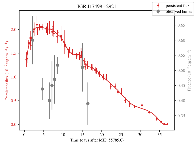
Figure 1: Observations of IGR J17498$-$2921 by RXTE/PCA, INTEGRAL/ISGRI and Swift/XRT during the 2011 outburst. The persistent flux in the 0.1–300 keV band estimated from spectral fits by Falanga et al. (2012) are shown as red points, and the observed burst fluences are shown as grey. Error bars indicate the $1\sigma$ uncertainties. Note the much longer duration of the outburst, and the larger number of detected bursts, compared to SAX J1808.4$-$3658. The spline approximation (smooth=0.1) used to integrate the persistent flux between bursts for the purposes of burst simulation is indicated as the solid red line.

3.3 Simulations

The simulation approach involves three principal steps. First, identifying a suitable parameter vector as a start point. The primary input parameters to the model are the hydrogen fraction $X$ and CNO metallicity $Z$; the base flux $Q_{b}$; the distance $d$ and anisotropy factors $\xi_{b}$ and $\xi_{p}$; and the neutron-star mass $M_{\rm NS}$ and radius $R_{\rm NS}$. The “systematic” error multipliers on the $\alpha$ and fluence values are two additional optional parameters, that are not used in the runs presented here (except where specified).

A qualitatively good initial solution will approximately replicate the burst history, including the burst times and number. Because the beansp code works both forward and backward in time from a “reference” burst, some adjustment of the reference burst choice (ref_ind) and the number of bursts to simulate (numburstssim) may also be required. For SAX J1808.4$-$3658, this exercise is trivial, as we can use the derived parameters from G19, along with the same parameters.

Second, running the MCMC sampler and identifying promising solution regions. Typically, running the sampler with 200 walkers for up to 1000 steps will provide a balance between run time and exploration of the parameter space. As the burst rate varies for different walker positions, the total number of bursts simulated at each step may also vary. Promising solution regions can be identified by plotting the burst predictions (which are divided up automatically as part of the do_analysis method based on the burst number) and comparing the RMS error between the average predicted burst times and the observations.

A key feature of this simulation approach is the necessity to match the predicted bursts with those observed. Because the data coverage is usually incomplete, there is a high probability of some bursts being missed; e.g. the pair of bursts inferred to have occurred between the first and second observed bursts in the 2002 outburst of SAX J1808.4$-$3658 (G19, Galloway & Cumming 2006). To compare the observed burst properties with the predictions, a burst in the predicted sequence must be selected for each observed event. The beansp code achieves this by selecting the mapping that minimises the RMS offset between the observed times and the predicted times for the selected bursts. However, as the walker positions evolve during the simulation, the mapping will sometimes change from step to step, likely introducing discontinuities in the likelihood hypersurface. Practically the consequences are that the confidence regions may be strongly multi-modal, and caution must be taken to ensure that the globally best-fit solution has been achieved.

Third, refining the walker ensemble to focus on the preferred solution. The user can “prune” the set of walkers after a preliminary run to remove those with sub-optimal burst matching sequences, and continue the simulation to fully explore the parameter space around the best identified solution.

The beansp code can take advantage of multi-core CPUs by using the threads option to run in parallel for as many threads as are available. The walker positions are adjusted each step with the emcee default “stretch move” of Goodman & Weare (2010), with default scale parameter $a=2.0$. For many of the runs presented here, the sampler gave an error which we understand is related to an insufficiently low fraction of successful moves (the average acceptance fraction at the end of the “base” runs for each source was 7–8%). We overcame this issue by successively reducing the scale factor in steps as $a^{\prime}=a/2+1/2$ (i.e. 1.5, 1.25, 1.125 etc). Typically the runs were completed with $a=1.25$.

4 Results

Here we describe the results from our simulations. In each case, the run parameters and posterior samples are available as accompanying data with the paper, at the companion repository site (see the “data availability” section).

4.1 SAX J1808.4–3658

We repeated the analysis of G19, running the MCMC sampler with 500 walkers and (initially) 2000 steps. We omitted the $\alpha$ values in the likelihood, for the reasons described in §2 (see also below). We also omitted the multiplicative factor for the fluence uncertainties.

We could not replicate the calculated autocorrelation times from G19; for our runs the initial values cluster around $\tau=10$ initially, rising linearly seemingly independent of the length of the run, and not reaching the target criteria even well beyond the 2000 steps of the previous runs. For that reason, we continued the MCMC chains for 8000 additional steps, for a total of 10000, and retained the last 1000 steps for the posteriors. The estimated $\tau\approx 1000$ by the end of this run, so still not meeting the rule-of-thumb for convergence.

The average of the predicted burst times and fluences match the observations well, with a residual RMS of 1.37 min (Fig. 2). This agreement is somewhat remarkable given the adopted error on the burst time of 10 min; in fact from the PCA data the start time of the bursts can be constrained to well under 1 s. As with previous analyses, we predict the occurrence of two additional bursts between the first two observed bursts; the predicted times fell within intervals during which no observations were available, so are still consistent with the observations. We estimated the recurrence time for the second observed burst from the difference of it’s observed time and the time of the third predicted burst (Table 1).

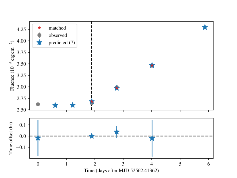
Figure 2: Comparison of observed and MCMC ensemble burst times and fluences for SAX J1808.4$-$3658 during the 2002 outburst. The top panel plots fluence as a function of burst times; the predicted bursts (blue stars) chosen for comparison with the observed bursts (grey circles) are additionally marked by a red star. Note the unobserved bursts between the first two observed events, and following the fourth. These events would have fallen during data gaps. The “reference” burst (from which the simulation proceeds both forward and backward in time) is marked as the black dashed line The lower panel shows the residuals between the observed and predicted times. There is no error on the second observed burst, as it is the reference for the simulations and hence is trivially identical to the observed time.

The calculated posteriors are broadly consistent with those of the previous analysis (Fig. 3). We find again the correlation between $X$ and $Z$ first noted by Galloway & Cumming (2006), although interestingly the track in the $X$–$Z$ plane has shifted to higher $Z$ values. We attribute this shift to the changes made to the code and the comparison algorithm, as described in §2.

Comparing the tabulated values, we note the posterior ranges have substantial overlap with the previous ranges (Table 2). We find that the hydrogen fraction $X$ is now much better constrained, with the value of $X=0.36$ having the maximum likelihood. The mass is instead shifted to much higher values, centred around $2.1\ M_{\odot}$; along with the slightly higher radius, these parameters lead to higher values of the surface gravity $g$ and redshift $1+z$, although not significantly discrepant from the previous analysis. The implied distance is somewhat closer, at $2.7\pm 0.3$ kpc. We also note a higher value for the burst anisotropy $\xi_{b}$, which could be the principal reason for the correspondingly lower distance.

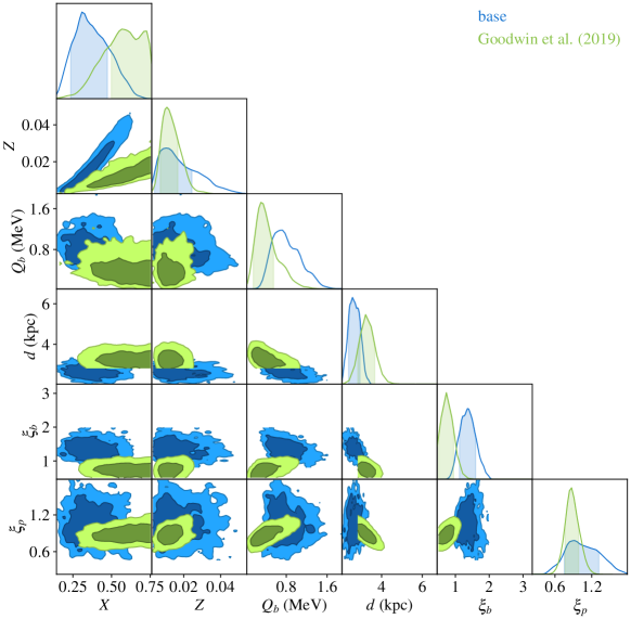
Figure 3: Two-dimensional posterior probabilities for the system parameters for SAX J1808.4$-$3658. The blue distributions show the results for our “base” run as described in §4.1, while the green distributions are those of G19. The displayed confidence contours within each 2-D panel are at 1 and $2\sigma$. The displayed parameters are the hydrogen mass fraction $X$, metallicity $Z$, base flux $Q_{\rm b}$, distance $d$, and the emission anisotropy parameters $\xi_{b}$ and $\xi_{p}$.

We revisit here the choice to omit the $\alpha$-values from the model-observation comparison. The measured values are generally derived from the persistent flux of the observation in which they occurred (see Table 1); this quantity may not cover the entire interval from the previous burst. Furthermore, for some events the inferred recurrence time may be subject to uncertainties from the number of missed bursts since the previous event. Also in Table 1 we compare the measured $\alpha$-values with the calculation incorporating both the model-predicted recurrence time (since the previous burst, whether observed or predicted) and the variations in the persistent flux over the entire interval (according to our flux model). We calculated the $\alpha$-values and propagated the uncertainties using routines from the concord suite of tools Galloway et al. (2022). We note that the measured values substantially underestimate the model-informed values, which further supports our choice (at least in this case) to omit them from the likelihood calculation.

Table 1: Measured and inferred properties for bursts from SAX J1808.4$-$3658 during the 2002 outburst, augmented by the model predictions. We infer the presence of two additional bursts between the first two observed events; hence, the recurrence time $\Delta t$ for the second event depends on the predictions, and thus introduces uncertainties. Similarly, the $\alpha$-values include this uncertainty, as well as the variation in persistent flux according to the model.

	MINBAR	Start	$\Delta t$	Fluence	$\alpha$-value
Burst	ID	(MJD)	(hr)	$10^{-6}\ {\rm erg\,cm^{-2}}$	Measured	Inferred
1	3037	52562.41362	…	$2.620\pm 0.021$	…	…
2	3038	52564.30514	$16.13\pm 0.05$	$2.649\pm 0.018$	$107.0\pm 2.0$	$117.5\pm 0.9$
3	3039	52565.18427	21.10	$2.990\pm 0.017$	$105.7\pm 1.9$	$121.7_{-0.6}^{+0.8}$
4	3040	52566.42677	29.82	$3.460\pm 0.022$	$121.1\pm 2.3$	$130.2\pm 0.8$

Table 2: System parameters for SAX J1808.4$-$3658 and IGR J17498$-$2921 derived from the burst comparison.

Parameter	SAX J1808.4$-$3658	IGR J17498$-$2921	Units
$X$	$0.36^{+0.13}_{-0.11}$	$0.15\pm 0.04$
$Z$	$0.016^{+0.014}_{-0.008}$	$0.0014^{+0.0004}_{-0.0003}$
$Q_{\rm b}$	$0.8^{+0.3}_{-0.2}$	$2.1^{+0.6}_{-0.5}$	MeV nucleon-1
$M$	$2.1^{+0.3}_{-0.4}$	$2.2^{+0.2}_{-0.4}$	$M_{\odot}$
$R$	$12.2\pm 0.9$	$12.0^{+0.9}_{-1.1}$	km
$g$	$2.5\pm 0.5$	$3.0^{+0.6}_{-0.5}$	$10^{14}\ {\rm cm\,s^{-2}}$
$1+z$	$1.41^{+0.08}_{-0.10}$	$1.48^{+0.07}_{-0.09}$
$d$	$2.7\pm 0.3$	$5.7^{+0.6}_{-0.5}$	kpc
$\xi_{p}$	$1.0^{+0.3}_{-0.2}$	$1.4\pm 0.20$
$\xi_{b}$	$1.4\pm 0.2$	$1.5^{+0.3}_{-0.2}$

4.2 IGR J17498–2921

The larger number of bursts for this source presented a much greater challenge for simulation. Falanga et al. (2012) suggested low inclination to explain the high $\alpha$ values, and we used this information (via the $\xi_{b}$ and $\xi_{p}$ parameters), along with the suggested distance range, to guide our initial choice of parameters.

The walkers in the early simulations tended to fragment into separate groups corresponding to different burst rates and consequently different mappings from the predicted to observed bursts. We gradually refined the available choices, prioritising the agreement on the burst time, for the final runs contributing to the parameter estimates here. For the final posteriors and model prediction ranges we chose a simulation running for 12,000 steps total, with 500 walkers. After 10,000 steps we “pruned” the set of walkers to retain only those which offered the best agreement in terms of the predicted times. The sub-optimal solutions, comprising only 5.7% of the walkers, had RMS time offsets of $>2$ hr, compared to $<1$ hr for the remainder. We replaced each of the walkers with sub-optimal solutios, with one chosen randomly from the set exhibiting better agreement, and ran for an additional 2,000 steps. For the final quantities and plots we discarded the initial 11,000 steps as burnin.

As before, the integrated autocorrelation time estimates did not indicate that the run had yet converged, as for SAX J1808.4$-$3658. The lack of convergence may be exacerbated by the low acceptance fraction for the walkers (see §3.3).

The comparison of predicted and observed times and fluences was good, with RMS 0.882 hr for the times (Fig. 4). However, the agreement was far from that of the SAX J1808.4$-$3658 bursts, and systematic variations apparently dominate the residuals. The observed variations in the fluences for the bursts from IGR J17498$-$2921 were also reproduced moderately well, generally consistent on average given the observational uncertainties. The predicted fluence was anticorrelated with the persistent flux (i.e. the inferred accretion rate).

The inferred burst recurrence times and $\alpha$-values are listed in Table 3. The burst recurrence times were also anticorrelated with the accretion rate, and varied between 13.85 hr at the peak of the outburst (between bursts 2 and 3) to 33.65 hr between bursts 7 and 8. The consistency of the $\alpha$ values around 250 for the main part of the burst train is perhaps a good indicator of reliability. As pointed out by Falanga et al. (2012), this value is well in excess of the maximum value expected for pure He bursts, of 150 (see also Galloway et al., 2022). However, the observed value also includes the ratio $\xi_{b}/\xi_{p}$, which according to the posteriors is $\approx 1.18$, bringing it closer to agreement.

It is interesting that the final observed burst in the train is at lower fluence than it’s predecessor, the opposite of the trend for the predicted bursts. In response the $\alpha$-value is even higher, around 400, and significantly in excess of the values earlier in the outburst. Although systematic effects and incorrect instrumental cross-calibration may affect the fluence measurement of this burst (observed with Swift), if the fluence is reliable it may indicate either that the burning is incomplete, or also that steady burning is removing a higher fraction of the accreted fuel than earlier in the outburst.

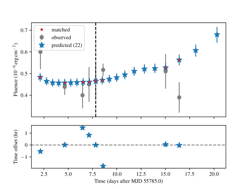
Figure 4: Comparison of observed and MCMC ensemble burst times and fluences for IGR J17498$-$2921 during the 2011 outburst. For this dataset the reference burst is chosen as the fifth observed event. The other details are as for Fig. 2

The system parameters appear to largely support the case for high inclination, with both $\xi_{b}$ and $\xi_{p}$ well in excess of 1 (Fig. 5). Interestingly, the preferred value of $\xi_{b}$ is in excess of typical ranges for the standard “model A”, and instead falls in the region traced by the flared trapezoidal (B) or triangular (C) model profiles of He & Keek (2016). The implied inclination is $60^{\circ}$ or higher, where the flared disk edge begins to obstruct the line of sight to the neutron star, substantially attenuating both the persistent and burst flux.

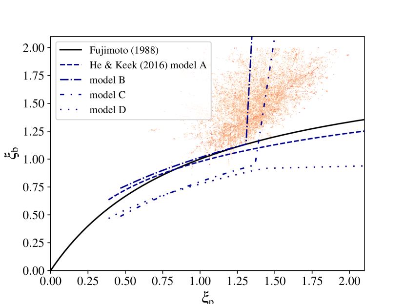
Figure 5: The distribution of burst and persistent emission anisotropy, $\xi_{b}$ and $\xi_{p}$ respectively, plotted against the predictions from analytic and numerical models. Note that the $\xi_{b}$ vlaue is generally in excess of the range spanned for thin or flared disks, instead suggesting a trapezoidal (B) or triangular (C) cross-sectional profile.

The implied composition for the burst fuel is both H- and CNO-poor (Fig. 6), with most remarkably the preferred $Z$ values an order of magnitude below solar. Perhaps to compensate, the implied base flux is higher than usually assumed, around 2 MeV nucleon^-1.

The distance posterior is centred around 5.7 kpc, which is somewhat closer than the range considered by Falanga et al. (2012). However, those authors did not take into account the emission anisotropy, which provides a significant correction given our best estimates. For that reason, we consider the closer distance more likely.

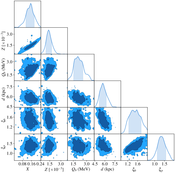
Figure 6: Two-dimensional posterior probabilities for the system parameters for IGR J17498$-$2921. Details as for Fig. 3

While the neutron-star radius is consistent with the canonical $\approx 12$ km value, the mass distribution is strongly skewed towards high values (Fig. 7). When combined with our inclination estimate and the the pulsar mass function $f(M_{2},M_{1},i)\simeq 2\times 10^{-3}\ M_{\odot}$ Papitto et al. (2011), the implied donor is lower mass, around $0.2\ M_{\odot}$, and must have significantly larger radius than a zero-age main sequence star of the same mass, in order to fill it’s Roche lobe.

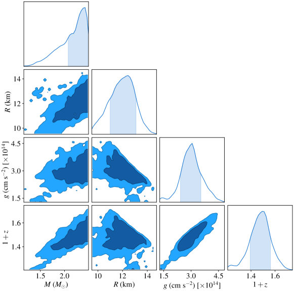
Figure 7: Two-dimensional posterior probabilities for the neutron star parameters for IGR J17498$-$2921.

Table 3: Measured and inferred properties for bursts from IGR J17498$-$2921 during the 2011 outburst, augmented by the model predictions.

	MINBAR	Start	$\Delta t$	Fluence	$\alpha$-value
Burst	ID	(MJD)	(hr)	$10^{-6}\ {\rm erg\,cm^{-2}}$	Measured	Inferred
1	8486	55787.13924	$18.92\pm 0.18$	$0.60\pm 0.08$	$160\pm 70$	$200_{-20}^{+30}$
2	8239	55789.64013	$14.88\pm 0.09$	$0.44\pm 0.04$	$310\pm 40$	$250_{-19}^{+23}$
3	8498	55791.47419	$13.85\pm 0.04$	$0.40\pm 0.06$	$320\pm 50$	$250_{-30}^{+40}$
4	8503	55792.14131	16.01	$0.45\pm 0.08$	$290\pm 60$	$260_{-40}^{+50}$
5	8508	55792.83207	16.58	$0.47\pm 0.08$	$270\pm 50$	$250_{-40}^{+50}$
6	8244	55793.5906	18.20	$0.52\pm 0.03$	$250\pm 20$	$244_{-13}^{+14}$
7	8526	55800.02405	$26.59\pm 0.16$	$0.51\pm 0.08$	$230\pm 40$	$270_{-40}^{+50}$
8	…	55801.42595	33.65	$0.39\pm 0.07$	$250\pm 50$	$400_{-60}^{+90}$

5 Discussion

We have made a detailed comparison of the predictions of an ignition model to 8 bursts observed from IGR J17498$-$2921 during it’s 2011 outburst, using the beansp code. We can broadly reproduce the behaviour with a model in which the accretion fuel is H-poor, with $X=0.15\pm 0.04$, and also low metallicity, at about a tenth of the solar value. The implied distance to the source is $5.7^{+0.6}_{-0.5}$ kpc, and the system is likely observed at an inclination of $\approx 60^{\circ}$, with indications that a “flared” accretion disk substantially attenuates both the burst and persistent luminosity towards our line of sight. The model predictions favour a massive neutron star, with $M\geq 2\ M_{\odot}$, and $R\approx 12$ km.

We achieved these constraints using an upgraded version of the beansp code, featuring substantial upgrades and improvements over the earlier versions. To quantify the effect of these changes, we have also re-analysed the observations of SAX J1808.4$-$3658 analysed by G19. We find that in general the new code produces comparable parameter confidence intervals, although we could not reproduce the autocorrelation times. Thus, the convergence of the MCMC chains remains uncertain.

We performed our comparisons on only the burst times and fluences, neglecting the estimated $\alpha$-values, as has been done in the past. By combining the predicted burst times with the observed fluences, we demonstrated that the $\alpha$ values estimated from the observations can have significant systematic errors, due to the varying persistent flux and uncertainties for the burst recurrence times.

We expect that the improvements in the code demonstrated here with the application to IGR J17498$-$2921 will enable further comparisons to burst trains from other sources.

5.1 Implications for the binary evolution of SAX J1808.4–3658 and IGR J17498–2921

In this work, we find that the accreted fuel composition in both binaries is hydrogen depleted. Given that the secondary star in both systems is low mass (0.05 M_⊙ and $>$0.16 M_⊙ respectively, Chakrabarty & Morgan 1998; Markwardt & Strohmayer 2011) this finding has important implications about the evolution of the binary systems. The present-day companions must represent the core of previously more massive stars. In order to deplete hydrogen in the core within the age of the Universe, both companion stars must have been significantly more massive than they are today, implying that they have lost a significant amount of mass via accretion to the neutron star in their lifetimes.

The binary evolution of SAX J1808.4$-$3658 was modelled by Goodwin & Woods (2020) taking into account the depleted hydrogen fraction of the companion star. Using the the Modules for Experiments in Stellar Astrophysics stellar evolution binary program (MESA; Paxton et al., 2015) to calculate evolutionary tracks of the binary system, they found that the companion star likely had an initial mass of 1.1 M_⊙, but at least $>0.6$ M_⊙.

Similarly for IGR J17498$-$2921, using MESA to evolve a single star for 14 billion yr, we deduce that the companion star must have been $>0.8$ M_⊙ in order to achieve a hydrogen fraction of 0.14 in its core within the age of the Universe. We plan more detailed simulation efforts in future to fully elucidate the evolutionary history of IGR J17498$-$2921 as well as SAX J1808.4$-$3658.

Data Availability

The data underlying this article are available in Monash University’s Bridges repository, at https://dx.doi.org/10.26180/24773367

References

- Alpar et al. (1982) Alpar M. A., Cheng A. F., Ruderman M. A., Shaham J., 1982, Nature, 300, 728
- Bult et al. (2019) Bult P., et al., 2019, ApJ, 885, L1
- Casten et al. (2023) Casten S., Strohmayer T. E., Bult P., 2023, ApJ, 948, 117
- Chakrabarty & Morgan (1998) Chakrabarty D., Morgan E. H., 1998, Nature, 394, 346
- Cumming & Bildsten (2000) Cumming A., Bildsten L., 2000, ApJ, 544, 453
- Di Salvo & Sanna (2022) Di Salvo T., Sanna A., 2022, in Bhattacharyya S., Papitto A., Bhattacharya D., eds, Astrophysics and Space Science Library Vol. 465, Astrophysics and Space Science Library. pp 87–124 (arXiv:2010.09005), doi:10.1007/978-3-030-85198-9_4
- Falanga et al. (2012) Falanga M., Kuiper L., Poutanen J., Galloway D. K., Bozzo E., Goldwurm A., Hermsen W., Stella L., 2012, A&A, 545, A26
- Ferrigno et al. (2011) Ferrigno C., Bozzo E., Belloni L. G. A. P. T. M., 2011, The Astronomer’s Telegram, 3560
- Foreman-Mackey et al. (2013) Foreman-Mackey D., Hogg D. W., Lang D., Goodman J., 2013, Publications of the Astronomical Society of the Pacific, 125, pp. 306
- Galloway & Cumming (2006) Galloway D. K., Cumming A., 2006, ApJ, 652, 559
- Galloway & Keek (2021) Galloway D. K., Keek L., 2021, Thermonuclear X-ray Bursts. pp 209–262 (arXiv:1712.06227), doi:10.1007/978-3-662-62110-3_5
- Galloway et al. (2006) Galloway D. K., Psaltis D., Muno M. P., Chakrabarty D., 2006, ApJ, 639, 1033
- Galloway et al. (2020) Galloway D. K., et al., 2020, ApJS, 249, 32
- Galloway et al. (2022) Galloway D. K., Johnston Z., Goodwin A., He C.-C., 2022, ApJS, 263, 30
- Goodman & Weare (2010) Goodman J., Weare J., 2010, CAMS, 5, 65
- Goodwin & Woods (2020) Goodwin A. J., Woods T. E., 2020, MNRAS, 495, 796
- Goodwin et al. (2019) Goodwin A. J., Galloway D. K., Heger A., Cumming A., Johnston Z., 2019, MNRAS, 490, 2228
- Goodwin et al. (2020) Goodwin A. J., et al., 2020, MNRAS, 498, 3429
- Grebenev et al. (2023) Grebenev S. A., Bryksin S. S., Sunyaev R. A., 2023, The Astronomer’s Telegram, 15996, 1
- He & Keek (2016) He C.-C., Keek L., 2016, ApJ, 819, 47
- Illiano et al. (2023) Illiano G., et al., 2023, ApJ, 942, L40
- Johnston et al. (2018) Johnston Z., Heger A., Galloway D. K., 2018, MNRAS, 477, 2112
- Linares et al. (2014) Linares M., et al., 2014, MNRAS, 438, 251
- Markwardt & Strohmayer (2011) Markwardt C. B., Strohmayer T. E., 2011, The Astronomer’s Telegram, 3601, 1
- Papitto et al. (2011) Papitto A., et al., 2011, A&A, 535, L4
- Papitto et al. (2014) Papitto A., Torres D. F., Rea N., Tauris T. M., 2014, A&A, 566, A64
- Patruno & Watts (2012) Patruno A., Watts A. L., 2012, preprint, (arXiv:1206.2727)
- Paxton et al. (2015) Paxton B., et al., 2015, ApJS, 220, 15
- Sanna et al. (2023) Sanna A., et al., 2023, The Astronomer’s Telegram, 15998, 1
- Tauris et al. (2012) Tauris T. M., Langer N., Kramer M., 2012, MNRAS, 425, 1601
- Virtanen et al. (2020) Virtanen P., et al., 2020, Nature Methods, 17, 261
- Wijnands & van der Klis (1998) Wijnands R., van der Klis M., 1998, Nature, 394, 344
- Worpel et al. (2013) Worpel H., Galloway D. K., Price D. J., 2013, ApJ, 772, 94
- Worpel et al. (2015) Worpel H., Galloway D. K., Price D. J., 2015, ApJ, 801, 60
- in ’t Zand et al. (1998) in ’t Zand J. J. M., Heise J., Muller J. M., Bazzano A., Cocchi M., Natalucci L., Ubertini P., 1998, A&A, 331, L25
- in ’t Zand et al. (2013) in ’t Zand J. J. M., et al., 2013, A&A, 553, A83