Certifiable lower bounds of Wigner negativity volume and
non-Gaussian entanglement with conditional displacement gates

Abstract

In circuit and cavity quantum electrodynamics devices where control qubits are dispersively coupled to high quality-factor cavities, characteristic functions of cavity states can be directly probed with echoed conditional displacement (ECD) gates. In this work, I propose a method to certify non-Gaussian entanglement between cavities using only ECD gates and qubit readouts. The ECD witness arises from an application of Bochner’s theorem to a surprising connection between two negativities: that of the reduced Wigner function, and that of the partial transpose. Non-Gaussian entanglement of some common states, like photon-subtracted two-mode squeezed vacua and entangled cats, can be detected by measuring as few as four points of the characteristic function. Furthermore, the expectation value of the witness is a simultaneous lower bound to the Wigner negativity volume and a geometric measure of entanglement conjectured to be the partial transpose negativity. Both negativities are strong monotones of non-Gaussianity and entanglement respectively, so the ECD witness provides experimentally-accessible lower bounds to quantities related to these monotones without the need for tomography on the cavity states.

I Introduction

Recent advances in both circuit and cavity quantum electrodynamics (cQED) has lead to a paradigm where continuous-variable (CV) computation is performed in high quality-factor cavities, such that operations on the quantum states of the cavities are mediated by qubits dispersively coupled to them [1, 2, 3, 4, 5, 6]. In systems with weak dispersive coupling, measurements with echoed conditional displacement (ECD) gates [7] can directly probe the pointwise characteristic function of the cavity states. Meanwhile, displaced parity measurements are possible but would take longer times, while quadrature measurements are unavailable.

As most CV entanglement witnesses are based on quadrature statistics [8, 9, 10], past demonstrations of entanglement in such architectures have instead resorted to violating Bell inequalities with measurements of different points of the Wigner function [11, 12] or by computing the entanglement fidelity from the tomographically-reconstructed state [13, 14, 15]. The former can be difficult in weakly-coupled systems due to the necessity of parity gates, while the latter is an expensive operation. Instead, an entanglement witness that uses only a few instances of ECD gates would be preferable in such setups.

Meanwhile, in the resource-theoretic studies of non-Gaussianity and entanglement, Wigner logarithmic negativity is a common measure used to quantify non-Gaussianity [16, 17], while logarithmic partial transpose negativity is a common measure that quantifies entanglement [18]. Apart from the property that they are non-Gaussian and entanglement monotones respectively, they are also favored in theoretical studies for their computability: the former only involves an integral over negative regions of the Wigner function, while the latter involves finding the eigenvalues of the partial transpose of a matrix. Given a state description, both can be easily calculated with numerical tools.

However, these quantities are difficult to obtain in experimental settings, as full tomography is required to reconstruct the state for either negativities to be calculated. Therefore, it is often desirable to instead find lower bounds to these quantities with just a few experimentally-accessible observables [19, 20].

The contributions of this work are twofold. First, I prove that a Wigner negativity witness based on Bochner’s theorem provides a lower bound to the Wigner negativity volume, which makes experimentally accessible a quantity often calculated in the resource-theoretic study of Wigner negativity and non-Gaussianity. To the best of my knowledge, existing Wigner negativity witnesses have only been shown to lower bound the trace distance of Wigner negativity, which, unlike the Wigner logarithmic volume, has not been shown to be a non-Gaussian monotone [21, 22].

Second, this work introduces a method to directly detect non-Gaussian entanglement between cavities using only ECD gates and qubit readouts. In most cases, very few settings of the ECD gates are needed for non-Gaussian entanglement to be certified: four for entangled Fock states, photon-subtracted two-mode squeezed vacua, and entangled cats.

These two contributions convene in the expected value of the proposed non-Gaussian entanglement witness, which simultaneously lower bounds the Wigner negativity volume and a geometric measure of entanglement of the state. The latter quantity is conjectured, and proven for a large family of states, to be equivalent to the partial transpose negativity.

Section II gives a brief background on the weak-dispersive regime of cQED systems and ECD gates, before the main results of this work are presented in Sec. III. Implementation details of the ECD witness, and its application to some example states, can be found in Sec. IV.

II Weak-dispersive Regime and ECD Gates

In the co-rotating frame of the free evolution of a cQED system, a qubit dispersively coupled to a driven cavity mode can be described by the Hamiltonian [23]

$$H(t)=-\frac{\hbar\chi}{2}a^{\dagger}a\sigma_{z}-\hbar Ka^{\dagger 2}a^{2}+\hbar\varepsilon^{*}(t)a+\hbar\varepsilon(t)a^{\dagger}+\cdots,$$ (1)

where $a$ is the creation operator of the cavity, $\sigma_{z}=\outerproduct{g}{g}-\outerproduct{e}{e}$ is Pauli Z on the qubit, $\chi$ is the cross-Kerr nonlinearity, $K$ is the self-Kerr nonlinearity, $\hbar\varepsilon(t)$ is the envelope of the time-dependent drive, and the ellipses contain higher-order terms.

As readout lines (control lasers) are coupled only to the qubit in circuit QED [2, 23] (cavity QED [3, 5, 6]), the only qubit measurements are available in both cases. Hence, to infer some properties of the cavity state from the qubit measurements, entangling operations between the qubit and the cavity are required. Such entangling operations typically have gate times of order $\sim\chi^{-1}$ [24].

On the other hand, to suppress the effects of higher-order terms, like the anharmonicity of the cavity, the Kerr nonlinearities, including $\chi$, have to be small in magnitude. This results in a trade-off between suppression of nonlinear effects and the length of entangling gate times.

A recent development offers an alternative to this trade-off. By setting the nonlinearities to be small and choosing an appropriate drive with a large amplitude, it is possible to induce the time evolution of the system to be a conditional displacement gate of the form [7]

$$U_{\text{ECD}}(\vec{\xi}):=D(\vec{\xi}/2)\outerproduct{e}{g}+D(-\vec{\xi}/2)\outerproduct{g}{e},$$ (2)

where $D(\vec{\xi})={\exp}(\sum_{k=1}^{M}\xi_{m}a_{m}^{\dagger}-\xi_{m}^{*}a_{m})=:{\exp}(\vec{\xi}\wedge\vec{a})$ is the usual $M$-mode displacement operator on the modes $\vec{a}$, with the shorthand $\vec{x}\wedge\vec{y}:=\sum_{k}[\vec{x}]_{k}[\vec{y}]_{k}^{\dagger}-[\vec{y}]_{k}[\vec{x}]_{k}^{\dagger}$. By initializing the qubit state to $\ket{+}\propto\ket{g}+\ket{e}$ so that the initial state of cavity and qubit system is $\rho\otimes\outerproduct{+}{+}$, then performing an ECD gate and measuring the qubit along the $\sigma_{x}=\outerproduct{g}{e}+\outerproduct{e}{g}$ or $\sigma_{y}=-i\outerproduct{g}{e}+i\outerproduct{e}{g}$ basis, the expectation values of $\sigma_{x}$ and $\sigma_{y}$ are

$$\expectationvalue{\sigma_{x}} =\tr[\sigma_{x}U_{\text{ECD}}(\vec{\xi})(\rho\otimes\outerproduct{+}{+})U^{\dagger}_{\text{ECD}}(\vec{\xi})]$$ (3)

$$=\real\!\Bqty{\tr[\rho D(\vec{\xi})]},$$

$$\expectationvalue{\sigma_{y}} =\tr[\sigma_{y}U_{\text{ECD}}(\vec{\xi})(\rho\otimes\outerproduct{+}{+})U^{\dagger}_{\text{ECD}}(\vec{\xi})]$$

$$=\imaginary\!\Bqty{\tr[\rho D(\vec{\xi})]},$$

from which ${\tr}[\rho D(\vec{\xi})]=\expectationvalue{\sigma_{x}}+i\expectationvalue{\sigma_{y}}$ can be obtained. This is the characteristic function of $\rho$, which is related to its Wigner function by a Fourier transform [25]

$$\tr[\rho D(\vec{\xi})]=\int\differential[2M]{\vec{\alpha}}W_{\rho}(\vec{\alpha})e^{\vec{\xi}\wedge\vec{\alpha}}.$$ (4)

The ECD gate time is of order $\sim[\chi\max_{t}\absolutevalue{\varepsilon(t)}]^{-1}$, so measuring each point of the characteristic function can be orders of magnitude faster than the $\sim\chi^{-1}$ of displaced parity gates required for the Wigner function [7, 24].

Both the characteristic and Wigner functions provide complete tomographic information of the cavity state, and entanglement can be deduced by obtaining either fully. However, as full tomography is an expensive procedure, it is desirable to deduce entanglement from just a few measurements. The rest of this work introduces a non-Gaussian entanglement witness based on measurements of the characteristic function, and hence one that can be easily implemented with ECD gates.

III Results

The ECD entanglement witness arises as a corollary of two theorems, whose proofs are given in Appendix A.

The first theorem is related to Bochner’s theorem, a result from harmonic analysis about the relationship between a nonnegative Wigner function and its Fourier transform [26, 27].

Theorem 1.

Certifiable Lower Bound of Wigner Negativity Volume. Given some phase-space points $\Xi:=\{\vec{\xi}_{k}\}_{k=1}^{N}$, define the matrix $\mathbf{C}(\rho,\Xi)$ with elements

$$[\mathbf{C}(\rho,\Xi)]_{j,k}=\frac{1}{N}\tr[\rho D(\vec{\xi}_{j}-\vec{\xi}_{k})].$$ (5)

Denoting the smallest eigenvalue of $\mathbf{C}(\rho,\Xi)$ as $\lambda_{-}$, the quantity $\mathcal{N}_{C}(\rho,\Xi):=\max(0,-\lambda_{-})$ is a lower bound for the Wigner negativity volume $\mathcal{N}_{V}(\rho)$ [28]:

$$\mathcal{N}_{C}(\rho,\Xi)\leq\mathcal{N}_{V}(\rho):=\frac{1}{2}\int\differential[2M]{\vec{\alpha}}\pqty\big{\absolutevalue{W_{\rho}(\vec{\alpha})}-W_{\rho}(\vec{\alpha})}.$$ (6)

Theorem 1 thus provides a method to lower bound the Wigner logarithmic negativity $\log[2\mathcal{N}_{V}(\rho)-1]$, which is a commonly-used monotone in the resource theories of non-Gaussianity and Wigner negativity [16, 17].

In a previous study of Bochner’s theorem as a negativity witness, Mari et al. [21] showed $\mathcal{N}_{C}(\rho,\Xi)$ to be a lower bound for the geometric measure $\mathcal{N}_{\tr}(\rho):=\min_{\sigma:W_{\sigma}\geq 0}\|\sigma-\rho\|_{1}$ based on the trace distance $\|\sigma-\rho\|_{1}=\tr|\sigma-\rho|$. As will be seen in later examples, $\mathcal{N}_{C}$ is a tighter bound for $\mathcal{N}_{V}$ than $\mathcal{N}_{\tr}$ for a few common states.

Note that Bochner’s theorem guarantees the existence of some $\Xi$ such that $\mathcal{N}_{C}(\rho,\Xi)>0$ for every $\rho$ with $\mathcal{N}_{V}(\rho)>0$ [26, 27]. Hence, the possible choices of $\Xi$ define a collection of negativity witnesses, for which every Wigner-negative state can be detected by at least one of them. This therefore forms a complete family of Wigner negativity witnesses [22].

The second theorem is a surprising connection between the negativity of the Wigner function and the negativity of the partial transpose.

Theorem 2.

Reduced Wigner Negativity Implies Partial Transpose Negativity. Consider the equal bipartition of $M$ modes into $\vec{a}_{A}:=\{a_{m}\}_{m=1}^{M/2}$ and $\vec{a}_{B}:=\{a_{m}\}_{m=M/2+1}^{M}$. Denote the partial transpose of $\rho$ over the modes $\vec{a}_{B}$ as $\rho^{T_{B}}$, and the partial trace of $\rho$ over the collective modes $\vec{a}_{-}:=(\vec{a}_{A}-\vec{a}_{B})/\sqrt{2}$ as $\tr_{-}\rho$. Then, negativities in the Wigner function of $\tr_{-}\rho$ implies negativities in $\rho^{T_{B}}$. That is,

$$W_{\tr_{-}\rho}(\vec{\alpha})\not\geq 0\implies\rho^{T_{B}}\not\succeq 0.$$ (7)

Although an equal bipartition was assumed, Theorem 2 can be trivially extended to an unequal bipartition $M_{A}>M_{B}$ by first performing a partial trace over $M_{A}-M_{B}$ modes in $\vec{a}_{A}$.

The two negativities were previously shown to be equivalent for a family of highly-symmetric pure states [29], while the nonnegativity of the reduced Wigner function over a collective mode was known for general product states in the context of quantum convolutions [27, 30], and later extended to separable states via convexity [31]. Theorem 2 thus subsumes the previous results about product and separable states [27, 30, 31], while Hudson’s theorem and a restriction to highly-symmetric pure states imply the result by Dahl et al. [29] (see Appendix B).

The preceding theorems imply the following corollary.

Corollary.

Certifiable Lower Bounds of Non-Gaussian Entanglement. Consider the equal bipartition of the $M$ total modes into $\vec{a}_{A}$ and $\vec{a}_{B}$. Choose some pairs of phase-space points $\Xi=\{(\vec{\xi}_{k}^{A},\vec{\xi}_{k}^{B})\}_{k=1}^{N}$, where every pair is symplectically related as

$$\forall k:\pmqty{undef}=\Lambda\pmqty{undef}$$ (8)

by the same $\Lambda$ for all $k$ such that $\Lambda^{\dagger}\spmqty{undef}\Lambda=\spmqty{undef}$. Then, define the matrix $\mathbf{C}_{2}(\rho,\Xi)$ with elements

$$[\mathbf{C}_{2}(\rho,\Xi)]_{j,k}=\frac{1}{N}\tr[\rho D_{A}(\vec{\xi}_{j}^{A}-\vec{\xi}_{k}^{A})D_{B}(\vec{\xi}_{j}^{B}-\vec{\xi}_{k}^{B})],$$ (9)

where $D_{A}(\vec{\xi})$ ($D_{B}(\vec{\xi})$) is the displacement operator over the $\vec{a}_{A}$ ($\vec{a}_{B}$) modes. Denoting the smallest eigenvalue of $\mathbf{C}_{2}(\rho,\Xi)$ as $\lambda_{-}$, the quantity $\mathcal{E}_{C}(\rho,\Xi):=\max(0,-\lambda_{-})$ lower bounds the following measures of entanglement

$$\mathcal{E}_{C}(\rho,\Xi)\leq\mathcal{E}_{\operatorname{SEP}}(\rho) :=\min_{\sigma\in\operatorname{SEP}}\|\sigma-\rho\|_{1},$$ (10)

$$\mathcal{E}_{C}(\rho,\Xi)\leq\mathcal{E}_{\operatorname{PPT}}(\rho) :=\min_{\sigma\in\operatorname{PPT}}\|\sigma^{T_{B}}-\rho^{T_{B}}\|_{1},$$

where $\operatorname{SEP}$ and $\operatorname{PPT}$ are respectively the set of separable states and positive-partial-transpose states over the $\vec{a}_{A}$–$\vec{a}_{B}$ bipartition.

Here, $\mathcal{E}_{\operatorname{SEP}}(\rho)$ is a familiar geometric measure defined as the distance between $\rho$ and the set of separable states [32]. It is not itself an entanglement monotone [33], although it can bound other measures that are [34]. Meanwhile, $\mathcal{E}_{\operatorname{PPT}}(\rho)$ is a similar geometric measure conjectured to be equivalent to the partial transpose negativity $\tr|\rho^{T_{B}}|-1$ [35]. The equivalence has been proven for a large class of states, including Schmidt-correlated states $\rho=\sum_{j,k}\rho_{j,k}\outerproduct{\psi_{j},\phi_{j}}{\psi_{k},\phi_{k}}$ and states with positive binegativity $\rho:|\rho^{T_{B}}|^{T_{B}}\succeq 0$ [35, 36]. Unlike $\mathcal{E}_{\operatorname{SEP}}(\rho)$, $\log\tr|\rho^{T_{B}}|$ is strongly monotonic [18].

By Theorem 1, $\mathcal{E}_{C}(\rho,\Xi)$ also lower bounds the Wigner negativity volume of $\rho$. Therefore, $\mathcal{E}_{C}>0$ simultaneously witnesses the Wigner negativity and entanglement of non-Gaussian entangled states, and provides quantitative lower bounds for some common measures of both.

Lastly, to consider how error bars in the experimental data will be propagated to $\mathcal{E}_{C}$, take that the data is reported to be $|\hat{d}_{j,k}-d_{j,k}|\leq\delta_{j,k}$ within a certain confidence level, where $\hat{d}_{j,k}$ ($d_{j,k}$) is the estimator (estimand) of $\langle D_{A}(\vec{\xi}_{j}^{A}-\vec{\xi}_{k}^{A})D_{B}(\vec{\xi}_{j}^{B}-\vec{\xi}_{k}^{B})\rangle$. Hence, the matrix $\mathbf{C}_{2}$ can be written as $\widehat{\mathbf{C}}_{2}=\mathbf{C}_{2}+\Delta$, where $[\widehat{\mathbf{C}}_{2}]_{j,k}=\hat{d}_{j,k}/N$, $[{\mathbf{C}}_{2}]_{j,k}=d_{j,k}/N$, and $[\Delta]_{j,k}$ can take any value within the radius $|[\Delta]_{j,k}|\leq\delta_{j,k}/N$. Writing the minimum eigenvalues of $(\widehat{\mathbf{C}}_{2},\mathbf{C}_{2},\Delta)$ as $(\hat{\lambda}_{-},\lambda_{-},\delta_{-})$, and the maximum eigenvalue of $\Delta$ as $\delta_{+}$, Weyl’s inequalities state that [37]

$$-\hat{\lambda}_{-}+\delta_{-}\leq-\lambda_{-}\leq-\hat{\lambda}_{-}+\delta_{+}.$$ (11)

Using Gershgorin circle theorem on $\Delta$ [37],

$$\absolutevalue{\max\delta_{+}},\absolutevalue{\min\delta_{-}}\leq\max_{j}\sum_{k\neq j}\frac{\delta_{j,k}}{N}=:\delta.$$ (12)

Hence, the widest range of Eq. (11) consistent with the experimental data and the reported error is $|\hat{\lambda}_{-}-\lambda_{-}|\leq\delta$. Therefore, within the given confidence level, the system is certain to be entangled when $\widehat{\mathcal{E}}_{C}>\delta$, and the experimental error bars are propagated to the computed lower bound as $\mathcal{E}_{C}=\widehat{\mathcal{E}}_{C}\pm\delta$.

IV The ECD Entanglement Witness

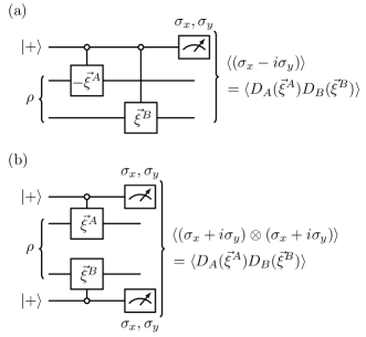
Figure 1: Circuit to measure the matrix elements $[\mathbf{C}_{2}]_{j,k}=\langle{D_{A}(\vec{\xi}_{j}^{A}-\vec{\xi}_{k}^{A})D_{B}(\vec{\xi}_{j}^{B}-\vec{\xi}_{k}^{B})}\rangle/N$, with (a) one or (b) two auxiliary qubits. The former requires less qubits and qubit measurements, while the latter requires only local gates and local measurements on the $A$ and $B$ subsystems. ECD gates $U_{\text{ECD}}(\alpha)$ are drawn as controlled unitary gates, where the open circles $\circ$ label the control qubit input and the target unitary are boxes containing the displacement argument $\vec{\xi}$. Note the negative signs in (a) due to an accumulated phase from chaining two ECD gates.

The ECD entanglement witness can be implemented with the following steps:

(1) Choose $N$ phase-space pairs $\Xi=\{(\vec{\xi}_{k}^{A},\vec{\xi}_{k}^{B})\}_{k=1}^{N}$ where $\vec{\xi}_{k}^{A}$ and $\vec{\xi}_{k}^{B}$ are symplectically related as per Eq. (8).

(2) Using ECD gates and qubit measurements (see Fig. 1), measure $\langle{D_{A}(\vec{\xi}^{A}_{j}-\vec{\xi}^{A}_{k})D_{B}(\vec{\xi}^{B}_{j}-\vec{\xi}^{B}_{k})}\rangle$ for all $j<k$. Denote the experimental error bars as $\delta_{j,k}$.

(3) Construct $\mathbf{C}_{2}$ with the matrix elements $[\mathbf{C}_{2}]_{j,k}=\langle{D_{A}(\vec{\xi}^{A}_{j}-\vec{\xi}^{A}_{k})D_{B}(\vec{\xi}^{B}_{j}-\vec{\xi}^{B}_{k})}\rangle/N$ for $j<k$ from the previous step, while the other elements are given by $[\mathbf{C}_{2}]_{j,j}=1$ and $[\mathbf{C}_{2}]_{j,k}=[\mathbf{C}_{2}]_{k,j}^{*}$ for $j>k$.

(4) Calculate $\lambda_{-}$, the minimum eigenvalue of $\mathbf{C}_{2}$. Define $\mathcal{E}_{C}:=\max(0,-\lambda_{-})$ and $\delta:=\max_{j}\sum_{k\neq j}\delta_{j,k}/N$. If $\mathcal{E}_{C}>\delta$, then the system is entangled, and $\mathcal{E}_{C}\pm\delta$ is a lower bound to $\mathcal{N}_{V}$, $\mathcal{N}_{\tr}$, $\mathcal{E}_{\operatorname{SEP}}$, and $\mathcal{E}_{\operatorname{PPT}}$.

The circuit that measures $[\mathbf{C}_{2}]_{j,k}$, which requires a single instance of the ECD gate for each subsystem and up to two auxiliary qubits, is shown in Fig. 1. Notice that there is the freedom to either use collective measurements, which reduces the number of auxiliary qubits needed, or measurements local to each subsystem, which would be required to witness entanglement between remote subsystems.

In total, up to $n_{q}N(N-1)$ measurement settings are needed, where $n_{q}\in\{1,2\}$ is the number of auxiliary qubits. This takes into account the $2n_{q}$ qubit settings ($\sigma_{x}$, $\sigma_{y}$ for each qubit) and the $N(N-1)/2$ ECD gate settings ($\vec{\xi}_{j}-\vec{\xi}_{k}$ for $j<k$). The number of measurement settings can be reduced with symmetries in the choice of $\Xi$, which will be shown in the following examples.

IV.1 Choice of Phase-space Points

As $\mathcal{E}_{C}(\rho,\Xi)>0$ is a witness of non-Gaussian entanglement for any $\Xi$, a good choice of $\Xi$ is one such that $\mathcal{E}_{C}$ is large for the target state $\rho$. This would ensure that the observed value of $\mathcal{E}_{C}$ would still be positive within experimental error bars, even with imperfect state preparation.

IV.1.1 Heuristic Maximization of Lower Bound

The best choice of phase-space points would be $\Xi_{\text{max}}$ such that $\mathcal{E}_{C}(\rho,\Xi_{\text{max}})=\max_{\Xi}\mathcal{E}_{C}(\rho,\Xi)$. However, closed form expressions of $\mathcal{E}_{C}$ tend to be unwieldy—if even obtainable—which can be difficult to optimize globally.

Instead, an initial heuristic choice $\Xi=\{(\vec{\xi}_{k}^{A},\vec{\xi}_{k}^{B})\}_{k=1}^{N}$ can be improved via gradient descent on the minimum eigenvalue $\lambda_{-}$ of $\mathbf{C}_{2}(\rho,\Xi)$. For simplicity, take the symplectic matrix $\Lambda$ in Eq. (8) to be fixed. Then, the partial derivative of $\lambda_{-}$ with respect to $\vec{\xi}_{k}^{A}$ is [38]

$$\frac{\partial\lambda_{-}}{\partial\vec{\xi}^{A*}_{k}}=\frac{\vec{v}^{\dagger}(\partial\mathbf{C}_{2}/\partial\vec{\xi}^{A*}_{k})\vec{v}}{\vec{v}^{\dagger}\vec{v}},$$ (13)

where $\vec{v}$ is the minimum eigenvector such that $\mathbf{C}_{2}\vec{v}=\lambda_{-}\vec{v}$, and $\partial\mathbf{C}_{2}/\partial\vec{\xi}^{A*}_{k}$ can be found by taking the partial derivative of each matrix element of $\mathbf{C}_{2}$.

For a small step size $\gamma>0$, the update $\forall k:\vec{\xi}_{k}^{A}\to\vec{\xi}_{k}^{A}-\gamma\partial\lambda_{-}/\partial\vec{\xi}^{A*}_{k}$ decreases the minimum eigenvalue of $\mathbf{C}_{2}(\rho,\Xi)$. This can be performed iteratively until the magnitude of the gradient $\sum_{k}|\partial\lambda_{-}/\partial\vec{\xi}^{A*}_{k}|^{2}$ is below a certain threshold, upon which a local minimum of $\mathcal{E}_{C}$ is approximately reached.

IV.1.2 Transformation Under Local Gaussian Unitaries

There are scenarios where an optimal choice of $\Xi$ for a state $\rho$ was already found from a prior optimization, and one would now be interested in witnessing the non-Gaussian entanglement of another state $\widetilde{\rho}$ sympletically related in some way to $\rho$. That is, $\widetilde{\rho}=U_{+}U_{-}U_{A}U_{B}\rho U_{B}^{\dagger}U_{A}^{\dagger}U_{-}^{\dagger}U_{+}^{\dagger}$ via Gaussian unitaries $U_{\mu}$ for $\mu\in\{A,B,+,-\}$, where [39]

$$\pmqty{undef}=\Lambda_{\mu}\pmqty{undef}+\pmqty{undef}$$ (14)

for some symplectic $\Lambda_{\mu}$, and

$$\pmqty{undef}:=\frac{1}{\sqrt{2}}\pmqty{undef}\pm\frac{1}{\sqrt{2}}\,\Lambda\pmqty{undef}$$ (15)

for the symplectic $\Lambda$ in Eq. (8) that relates $\vec{\xi}_{k}^{A}$ with $\vec{\xi}_{k}^{B}$. Substituting this into $\mathbf{C}_{2}(\rho,\Xi)$,

$${}[\mathbf{C}_{2}(\rho,\Xi)]_{j,k} =\tr_{+}\bigg{\{}U_{+}\Big{[}U_{A}D_{A}(\vec{\xi}_{j}^{A}-\vec{\xi}_{k}^{A})U_{A}^{\dagger}$$ (16)

$$\qquad\qquad\qquad{}\times{}U_{B}D_{B}(\vec{\xi}_{j}^{B}-\vec{\xi}_{k}^{B})U_{B}^{\dagger}\Big{]}U_{+}^{\dagger}$$

$$\qquad\qquad\qquad\qquad\qquad{}\times{}\tr_{-}\pqty{U_{-}^{\dagger}\widetilde{\rho}U_{-}}\bigg{\}}$$

$$=\tr[D_{A}(\widetilde{\xi}_{j}^{A}-\widetilde{\xi}_{k}^{A})D_{B}(\widetilde{\xi}_{j}^{B}-\widetilde{\xi}_{k}^{B})\widetilde{\rho}]$$

$$\qquad\qquad\qquad{}\times{}e^{\widetilde{\alpha}^{A}_{0}\wedge(\widetilde{\xi}_{j}^{A}-\widetilde{\xi}_{k}^{A})}e^{\widetilde{\alpha}^{B}_{0}\wedge(\widetilde{\xi}_{j}^{B}-\widetilde{\xi}_{k}^{B})}$$

$$=[\mathbf{C}_{2}(\widetilde{\rho},\widetilde{\Xi})]_{j,k}\;e^{\widetilde{\alpha}^{A}_{0}\wedge(\widetilde{\xi}_{j}^{A}-\widetilde{\xi}_{k}^{A})}e^{\widetilde{\alpha}^{B}_{0}\wedge(\widetilde{\xi}_{j}^{B}-\widetilde{\xi}_{k}^{B})},$$

where $\tr_{\pm}$ is the partial trace over the $\vec{a}_{\pm}$ modes. Here, I have also defined $\widetilde{\Xi}:=\{(\widetilde{\xi}_{k}^{A},\widetilde{\xi}_{k}^{B})\}_{k=1}^{N}$, where $\widetilde{\xi}_{k}^{\mu}$ and $\widetilde{\alpha}_{0}^{\mu}$ for $\mu\in\{A,B\}$ are given by

$$\pmqty{undef}=\Lambda_{+}\Lambda_{\mu}\pmqty{undef},\pmqty{undef}=\Lambda_{+}\pmqty{undef}+\pmqty{undef}.$$ (17)

The phase factors in the last line of Eq. (16) act as a unitary transformation on $\mathbf{C}_{2}(\widetilde{\rho},\widetilde{\Xi})$, which leaves the minimum eigenvalue unchanged. Therefore,

$$\mathcal{E}_{C}(\widetilde{\rho},\widetilde{\Xi})=\mathcal{E}_{C}(\rho,\Xi),$$ (18)

so the ECD witness can be also be used to detect $\widetilde{\rho}$ with the same expected value of $\mathcal{E}_{C}$ by simply choosing the phase-space pairs $\widetilde{\Xi}$ instead of $\Xi$.

IV.2 Examples

In this section, the witness is applied to some common non-Gaussian entangled states. The heuristically-optimized values of $\mathcal{E}_{C}(\rho,\Xi)$ are plotted for these states, and compared against the other measures of Wigner negativity and entanglement. Details on obtaining the other measures for the example states can be found in Appendix C. The choice of phase-space points $\Xi$ are also reported for the simplest cases. For brevity, $\Xi=\{(\vec{\xi}_{k}^{A}=\vec{\xi}_{k},\vec{\xi}_{k}^{B}=\vec{\xi}_{k})\}_{k=1}^{N}$ will be written as $\Xi=\{\vec{\xi}_{k}\}_{k=1}^{N}$ in the sections that follow.

IV.2.1 Entangled Single-photon Fock States

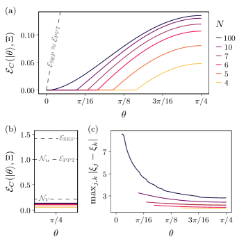
Figure 2: Entangled single-photon Fock states. (a) Expectation value $\mathcal{E}_{C}$ of the ECD witness against $\theta$. $\mathcal{E}_{\text{SEP}}\approx\mathcal{E}_{\text{PPT}}\approx 2\theta$ for $\theta\ll 1$ is plotted as a gray dashed line, while both $\mathcal{N}_{V}$ and $\mathcal{N}_{\tr}$ are outside plot range. Non-Gaussian entanglement is detected for $\theta\gtrsim 0.01\pi$ with $N=100$, and for $\theta\gtrsim 0.146\pi$ with $N=4$. (b) Same plot in the neighborhood of $\theta=\pi/4$, with the vertical axis expanded to show all negativity and entanglement measures. Notice in particular that $\mathcal{E}_{C}$ is a tighter bound for $\mathcal{N}_{V}$ than for $\mathcal{N}_{\tr}$, and $\mathcal{E}_{\operatorname{PPT}}$ than for $\mathcal{E}_{\operatorname{SEP}}$. (c) Maximum magnitude of the displacements required to implement the ECD witness, which scales approximately as $\sim(\theta-\pi/4)^{2}$.

The Fock state $\ket{1,0}$ passed through a beamsplitter gate $B(\theta):=e^{\theta(a_{1}^{\dagger}a_{2}-a_{1}a_{2}^{\dagger})}$ is given by

$$\ket{\theta}:=B(\theta)\ket{1,0}=\cos\theta\ket{1,0}+\sin\theta\ket{0,1},$$ (19)

which is entangled for any $\theta>0$ and maximally entangled at $\theta=\pi/4$.

Applying the ECD witness on $\ket{\theta}$, the expectation value $\mathcal{E}_{C}$ is plotted in Fig. 2(a), and compared in detail to the Wigner negativity and entanglement measures in the neighborhood of the maximally-entangled state $\ket{\theta=\pi/4}$ in Fig. 2(b). The measures $\mathcal{N}_{V}$, $\mathcal{N}_{\tr}$, $\mathcal{E}_{\operatorname{PPT}}$, and $\mathcal{E}_{\operatorname{SEP}}$ were all found analytically.

An immediate observation is that more measurements are required to detect the state at smaller angles: $\mathcal{E}_{C}>0$ for $\theta\gtrsim 0.146\pi$ with $N=4$, while $\mathcal{E}_{C}>0$ for $\theta\gtrsim 0.01\pi$ with $N=100$. Notice also that $\mathcal{E}_{C}$ is a tighter lower bound for $\mathcal{N}_{V}$ than $\mathcal{N}_{\tr}$, and for $\mathcal{E}_{\operatorname{PPT}}$ than $\mathcal{E}_{\operatorname{SEP}}$.

Figure 2(c) shows the maximum magnitude of the displacements needed when performing the ECD gates during the implementation of this witness. The dependence on $\theta$ is approximately quadratic, with the least displacement required when the state is maximally entangled.

For $N=4$, the phase-space points used in Fig. 2(a) are $\Xi=\{\pm\real[\xi_{0}],\pm i\imaginary[\xi_{0}]\}$, where

$$\xi_{0}{}={} i\Bqty{\frac{813}{1217}+\frac{\cos\!\bqty{\frac{1249}{171}\pqty{\frac{\pi}{4}-\theta}+\frac{2179}{215}\pqty{\frac{\pi}{4}-\theta}^{4}}}{1313}}$$ (20)

$$\quad{}+{}\frac{2531}{2745}+\frac{453}{2083}\pqty{\frac{\pi}{4}-\theta}^{2}.$$

For this choice of $\Xi$, the only displacements needed are $\xi_{j}-\xi_{k}\in\{2\real[\xi_{0}],i2\imaginary[\xi_{0}],2\xi_{0},2\xi_{0}^{*}\}$, as the other matrix elements of $\mathbf{C}_{2}$ can be obtained with $\langle{D(-\vec{\xi})}\rangle=\langle{D(\vec{\xi})}\rangle^{*}$. Thus, the non-Gaussian entanglement of $\ket{\theta}$ with $\theta\gtrsim 0.146\pi$ can be witnessed by measuring only four points of the characteristic function.

IV.2.2 Photon-subtracted Two-mode Squeezed Vacua

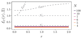
Figure 3: Photon-subtracted two-mode squeezed vacua. The expected value of the ECD witness and Wigner negativity measures are the same as for Fig. 2 at $\theta=\pi/4$, as this state is symplectically related to the maximally-entangled Fock state. Meanwhile, both entanglement measures increase with the amount of squeezing. Unlike before, $\mathcal{E}_{C}$ is not always a tighter bound for $\mathcal{E}_{\operatorname{PPT}}$, since $\mathcal{E}_{\operatorname{PPT}}>\mathcal{E}_{\operatorname{SEP}}$ for $r\gtrsim 0.25$. Generally, $\mathcal{E}_{C}$ is a rather loose bound for the entanglement measures, but it is also the case that $\mathcal{E}_{C}>0$ for all $r$, so the ECD witness can certify the non-Gaussian entanglement of all photon-subtracted two-mode squeezed vacua as defined in Eq. (21).

Photon-subtracted two-mode squeezed vacua, which can be prepared by postselecting on a photon-detection event on squeezed vacuum states, are of the form [40]

$$\ket{r} \propto B(\pi/4)\,a_{1}\,S_{1}(-r)S_{2}(r)\ket{0,0}$$ (21)

$$\propto(a_{1}+a_{2})\ket{\text{TMSV}(r)}$$

$$\propto S_{+}(-r)S_{-}(r)\ket{\theta=\pi/4},$$

where $B(\theta)$ is the beamsplitter gate from before, $S_{\mu}(r)=\exp[(r/2)(a_{\mu}^{2}-a_{\mu}^{\dagger 2})]$ is the squeeze operator for the mode $a_{\mu}\in\{a_{1},a_{2},a_{+},a_{-}\}$ with $a_{\pm}\propto a_{1}\pm a_{2}$, and $\ket{\text{TMSV}(r)}\propto\sum_{n=0}^{\infty}\tanh^{n}(r)\ket{n,n}$ is the two-mode squeezed vacuum.

The last line of Eq. (21) shows that $\ket{r}$ is symplectically related to the maximally-entangled Fock state from the previous section, so the Wigner negativity measures $\mathcal{N}_{V}$ and $\mathcal{N}_{\tr}$ for every $\ket{r}$ are the same as those for $\ket{\theta=\pi/4}$. Furthermore, using Eqs. (16) & (17), it is possible to obtain the same expected value $\mathcal{E}_{C}(\ket{r},\Xi_{r})=\mathcal{E}_{C}(\ket{\theta=\pi/4},\Xi)$ of the witness with

$$\Xi_{r}:=\{\real[\xi]e^{-r}+i\imaginary[\xi]e^{r}:\xi\in\Xi\}.$$ (22)

These quantities are plotted together with the entanglement measures in Fig. 3. Entanglement increases with squeezing parameter $r$, with $\mathcal{E}_{\operatorname{PPT}}\leq\mathcal{E}_{\operatorname{SEP}}$ for $r\lesssim 0.25$ and $\mathcal{E}_{\operatorname{PPT}}\geq\mathcal{E}_{\operatorname{SEP}}$ for $r\gtrsim 0.25$. Meanwhile, the value of $\mathcal{E}_{C}>0$ is the same for every $r$. On one hand, this means that it is a very loose lower bound for the entanglement measures, especially as $r$ increases. On the other hand, this also means that the ECD witness is able to witness the entanglement of a photon-subtracted two-mode squeezed vacuum state with any amount of squeezing.

IV.2.3 Entangled Cats

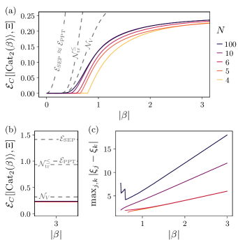
Figure 4: Entangled cats. (a) Expected value $\mathcal{E}_{C}$ of the ECD witness against $|\beta|$, with all Wigner negativity and entanglement measures also shown. $\mathcal{E}_{\text{SEP}}\approx\mathcal{E}_{\text{PPT}}$ only for $|\beta|\ll 1$. Non-Gaussian entanglement of every cat state with $|\beta|\gtrsim 3/4$ can be detected. (b) Plot expanded in the region around $|\beta|=3$. Notice again that $\mathcal{E}_{C}$ is a tighter bound for $\mathcal{N}_{V}$ than for $\mathcal{N}_{\tr}$, and $\mathcal{E}_{\operatorname{PPT}}$ than for $\mathcal{E}_{\operatorname{SEP}}$. (c) Maximum magnitude of ECD displacements, which scales linearly with $|\beta|$. The nonlinear variations at small $|\beta|$ are likely due to the small amount of Wigner negativities at those values, which are sensitive to the numerical precision during heuristic optimization.

Entangled cats are the form $\ket{\operatorname{Cat}_{2}(\beta)}\propto\ket{\beta,\beta}+\ket{-\beta,-\beta}$, where $\ket{\beta_{1},\beta_{2}}=D_{1}(\beta_{1})D_{2}(\beta_{2})\ket{0,0}$ are the usual coherent states.

The expectation value of the ECD witness applited to $\ket{\operatorname{Cat}_{2}(\beta)}$ is plotted in Fig. 4(a), and compared in detail to the other measures in the neighborhood of $|\beta|=3$ in Fig. 4(b). The entanglement measures $\mathcal{E}_{\operatorname{SEP}}$ and $\mathcal{E}_{\operatorname{PPT}}$ were found analytically, and the Wigner negativity volume $\mathcal{N}_{V}$ was computed with numerical integration, while only a lower bound $\mathcal{N}_{\tr}^{\leq}\leq\mathcal{N}_{\tr}$ could be obtained for the trace distance negativity.

Every cat state with $|\beta|\gtrsim 3/4$ can be detected with $N\geq 4$, while a larger $N$ is required to witness cat states of smaller magnitudes. Just like the entangled Fock states, $\mathcal{E}_{C}$ is once again a tighter lower bound for $\mathcal{N}_{V}$ than $\mathcal{N}_{\tr}$, and $\mathcal{E}_{\operatorname{PPT}}$ than $\mathcal{E}_{\operatorname{SEP}}$.

For $N=4$, the phase-space points used for the witness are $\Xi=\{\pm\xi_{+0},\pm\xi_{-0}\}$ with $\xi_{\pm 0}:=\beta+i\pi/(8\beta^{*})$. Hence, the only displacements needed are $\xi_{j}-\xi_{k}\in\{2\beta,i\pi/(4\beta^{*}),2\xi_{+0},2\xi_{-0}\}$, so the non-Gaussian entanglement of $\ket{\operatorname{Cat}_{2}(\beta)}$ with $|\beta|\gtrsim 3/4$ can also be witnessed with only four points of the characteristic function.

IV.3 Robustness of Witness Against Noise

As a case study of the effects of noise on the ECD witness, consider the noise channel

$$\mathcal{L}_{\eta}[\bullet]:=\tr_{\vec{b}}\{U_{\eta}[\bullet\otimes\outerproduct{0}{0}^{\otimes M}]U^{\dagger}_{\eta}\},$$ (23)

where $\vec{b}$ are the modes of the environment and $U_{\eta}\vec{a}U_{\eta}^{\dagger}=\sqrt{1-\eta}\vec{a}+\sqrt{\eta}\vec{b}$. This describes the loss of photons to the environment with some noise parameter $\eta$, where $\eta=0$ is the lossless case.

The performance of the witness in the presence of photon loss is plotted in Fig. 5 for the example states $\ket{\theta=\pi/4}$ and $\ket{\operatorname{Cat}_{2}(\beta=2)}$. Two scenarios with different choices of $\Xi$ are considered: where $\Xi$ of the lossless state is naïvely used (dotted traces), and where $\Xi$ has been further maximized for the noisy state (solid traces). The former scenario captures the case where noise is present but uncharacterized, in contrast to the latter scenario where the noise model is known.

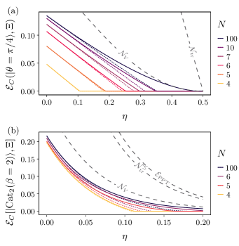
Figure 5: Performance of the ECD witness in the presence of photon loss for (a) the maximally-entangled Fock state $\ket{\theta=\pi/4}$ and (b) the entangled cat state $\ket{\operatorname{Cat}_{2}(\beta=2)}$. The Wigner negativity and entanglement measures not visible are beyond the limits of the graph. Two scenarios are plotted: where the phase-space points $\Xi$ of the lossless case is naïvely used even in the presence of noise (dotted traces), and where $\Xi$ have been further maximized for the noisy state (solid traces). The latter scenario captures the situation where the noise has been fully characterized. The ECD witness is robust in the presence of photon loss, even when the phase-space points are not further optimized with the knowledge of the noise model.

As seen in Fig. 5, the ECD witness is fairly robust against noise: even without further optimization of $\Xi$, it detects the non-Gaussian entanglement of $\ket{\theta=\pi/4}$ up to a photon loss of $\eta\lesssim 0.35$, and that of $\ket{\operatorname{Cat}_{2}(\beta=2)}$ up to $\eta\lesssim 0.19$. An even wider range of noisy states can be detected with $\Xi$ optimized for the characterized noise: in fact, $\mathcal{E}_{C}$ even saturates the Wigner negativity volume for $\ket{\theta=\pi/4}$ with photon loss $0.4\lesssim\eta<0.5$.

Note that the performance of the witness is of course dependent on the robustness of the state itself against noise. For example, the nonclassical features of the cat state are known to be sensitive to photon loss [41], which manifests in the exponential decay of all quantities plotted in Fig. 5(b). Recent theoretical and experimental efforts to mitigate the effect of photon loss have turned to squeezed cat states, which preserves these nonclassical features even at larger values of $\eta$ [42, 43, 44]. The ECD witness carries over easily to such squeezed cat states, as Eq. (14) can be used to find the new phase-space points with which to implement the witness.

V Conclusion

In this work, I have proposed a non-Gaussian entanglement witness that uses only ECD gates and qubit measurements. It does not require full or partial tomography, and is particularly suitable for weakly-dispersive cQED systems where quadrature measurements and parity gates are unavailable or prohibitively difficult.

Furthermore, the expected value of the witness is a lower bound to the Wigner negativity volume and a geometric measure of entanglement conjectured to be the partial transpose negativity. The Wigner and partial transpose negativities are non-Gaussian and entanglement monotones respectively, and are measures are commonly computed in the resource-theoretic studies of non-Gaussianity and entanglement. Estimating these measures in an experimental setting usually require tomography, which is an expensive operation. The ECD witness thus provides an experimentally-accessible method to lower bound quantities related to these measures.

Case studies for some common states, like entangled Fock states, photon-subtracted two-mode squeezed vacua, and entangled cats, show that they can be witnessed by measuring as few as four points of the characteristic function. In addition, the ECD witness is robust against photon loss, with or without any characterization of the noise present. It is also easily adaptable for states related by symplectic transformations, which makes it naturally applicable to noise mitigation techniques that were recently introduced in the literature.

While any Wigner negativity witness could be potentially used in tandem with Theorem 2 to certify non-Gaussian entanglement, the primary benefit of the ECD witness introduced in this work is the possibility for it to be implemented using local gates and local measurements. Contrast this, for example, with the family of witnesses introduced by Chabaud et al. [22]. A key part of detecting non-Gaussian entanglement with Theorem 2 requires detecting Wigner negativity in the collective mode $a_{+}\propto a_{1}+a_{2}$. With their witness, this requires measuring fidelities of the state against the collective Fock state $\ket{n}_{+}\propto\sum_{k=0}^{n}\sqrt{\binom{n}{k}}\ket{k}_{1}\otimes\ket{n-k}_{2}$, which is highly nonlocal in the $a_{1}$ and $a_{2}$ modes.

An open question that remains is the relationship between $\mathcal{E}_{C}$ and the partial transpose negativity. While the former is a lower bound for the latter for the example states studied, this relies on a yet-unproven conjecture about $\mathcal{E}_{\operatorname{PPT}}$ for more general states. As the ECD witness is not a fidelity witness, usual techniques that relate entanglement witnesses with quantitative estimates of the partial transpose negativity give trivial lower bounds [45].

Appendix A Proof of Theorems and Corollary

Theorem 1.

Certifiable Lower Bound of Wigner Negativity Volume. Given some phase-space points $\Xi:=\{\vec{\xi}_{k}\}_{k=1}^{N}$, define the matrix $\mathbf{C}(\rho,\Xi)$ with elements

$$[\mathbf{C}(\rho,\Xi)]_{j,k}=\frac{1}{N}\tr[\rho D(\vec{\xi}_{j}-\vec{\xi}_{k})].$$ (24)

Denoting the smallest eigenvalue of $\mathbf{C}(\rho,\Xi)$ as $\lambda_{-}$, the quantity $\mathcal{N}_{C}(\rho,\Xi):=\max(0,-\lambda_{-})$ is a lower bound for the Wigner negativity volume $\mathcal{N}_{V}(\rho)$ [28]:

$$\mathcal{N}_{C}(\rho,\Xi)\leq\mathcal{N}_{V}(\rho):=\frac{1}{2}\int\differential[2M]{\vec{\alpha}}\pqty\big{\absolutevalue{W_{\rho}(\vec{\alpha})}-W_{\rho}(\vec{\alpha})}.$$ (25)

Proof.

Using the fact that ${\tr}[\rho D(\vec{\xi})]$ is the Fourier transform of $W_{\rho}(\vec{\alpha})$, the matrix elements of $\mathbf{C}(\rho,\Xi)$ are

$$[\mathbf{C}(\rho,\Xi)]_{j,k}=\frac{1}{N}\int\differential[2M]{\vec{\alpha}}W_{\rho}(\vec{\alpha})e^{\vec{\xi}_{j}\wedge\vec{\alpha}}e^{-\vec{\xi}_{k}\wedge\vec{\alpha}}.$$ (26)

Recall that $\vec{\xi}\wedge\vec{\alpha}=\sum_{m=1}^{M}\alpha_{m}\xi_{m}^{*}-\alpha_{m}^{*}\xi_{m}$, which is antisymmetric with respect to conjugation $(\vec{\xi}\wedge\vec{\alpha})^{*}=-\vec{\xi}\wedge\vec{\alpha}$. Let $\vec{v}(\vec{\alpha}):=(e^{\vec{\xi}_{1}\wedge\vec{\alpha}},e^{\vec{\xi}_{2}\wedge\vec{\alpha}},\dots,e^{\vec{\xi}_{N}\wedge\vec{\alpha}})^{T}/\sqrt{N}$. Then,

$$\mathbf{C}(\rho,\Xi)=\int\differential[2M]{\vec{\alpha}}W_{\rho}(\vec{\alpha})\vec{v}(\alpha)\vec{v}^{\dagger}(\alpha),$$

with normalization $\lvert\vec{v}(\vec{\alpha})\rvert^{2}=1$. Hence, $0\leq\lvert\vec{u}^{\dagger}\vec{v}(\vec{\alpha})\rvert^{2}\leq\lvert\vec{u}\rvert^{2}$ by the Cauchy–Schwarz inequality [47].

Meanwhile, the Wigner function can be written as the difference $W_{\rho}(\vec{\alpha})=W_{\rho}^{+}(\vec{\alpha})-W_{\rho}^{-}(\vec{\alpha})$ of two nonnegative functions $\forall\vec{\alpha}:W_{\rho}^{\pm}(\vec{\alpha})\geq 0$. With this, the negativity volume is given by $\mathcal{N}_{V}(\rho)=\int\differential[2M]{\vec{\alpha}}\,W_{\rho}^{-}(\vec{\alpha})$, and

$$-\lambda_{\text{min}} =-\min_{\vec{u}:\absolutevalue{\vec{u}}^{2}=1}\vec{u}^{\dagger}\mathbf{C}(\rho,\Xi)\vec{u}$$ (27)

$$=\max_{\vec{u}:\absolutevalue{\vec{u}}^{2}=1}\int\differential[2M]{\vec{\alpha}}\Big{(}W_{\rho}^{-}(\vec{\alpha})\absolutevalue{\vec{u}^{\dagger}\vec{v}(\vec{\alpha})}^{2}$$

$$\qquad\qquad\qquad\qquad\qquad{}-{}W_{\rho}^{+}(\vec{\alpha})\absolutevalue{\vec{u}^{\dagger}\vec{v}(\vec{\alpha})}^{2}\Big{)}$$

$$\leq\max_{\vec{u}:\absolutevalue{\vec{u}}^{2}=1}\int\differential[2M]{\vec{\alpha}}\,W_{\rho}^{-}(\vec{\alpha})\absolutevalue{\vec{u}^{\dagger}\vec{v}(\vec{\alpha})}^{2}$$

$$\leq\underbrace{\max_{\vec{u}:\absolutevalue{\vec{u}}^{2}=1}\max_{\vec{\alpha}}\absolutevalue{\vec{u}^{\dagger}\vec{v}(\vec{\alpha})}^{2}}_{1}\underbrace{\int\differential[2M]{\vec{\alpha}}\,W_{\rho}^{-}(\vec{\alpha})}_{\mathcal{N}_{V}(\rho)}$$

$$=\mathcal{N}_{V}(\rho).$$

Together with the trivial condition $0\leq\mathcal{N}_{V}(\rho)$, it is therefore the case that $\mathcal{N}_{C}(\rho,\Xi)\leq\mathcal{N}_{V}(\rho)$, as desired. ∎

Theorem 2.

Reduced Wigner Negativity Implies Partial Transpose Negativity. Consider the equal bipartition of $M$ modes into $\vec{a}_{A}:=\{a_{m}\}_{m=1}^{M/2}$ and $\vec{a}_{B}:=\{a_{m}\}_{m=M/2+1}^{M}$. Denote the partial transpose of $\rho$ over the modes $\vec{a}_{B}$ as $\rho^{T_{B}}$, and the partial trace of $\rho$ over the collective modes $\vec{a}_{-}:=(\vec{a}_{A}-\vec{a}_{B})/\sqrt{2}$ as $\tr_{-}\rho$. Then, negativities in the Wigner function of $\tr_{-}\rho$ implies negativities in $\rho^{T_{B}}$. That is,

$$W_{\tr_{-}\rho}(\vec{\alpha})\not\geq 0\implies\rho^{T_{B}}\not\succeq 0.$$ (28)

Proof.

First, define the phase-space coordinates $\vec{\alpha}_{\pm}:=(\vec{\alpha}_{A}\pm\vec{\alpha}_{B})/\sqrt{2}$ of the collective modes $\vec{a}_{\pm}:=(\vec{a}_{A}\pm\vec{a}_{B})/\sqrt{2}$. The partial trace over $\vec{a}_{-}$ is given by the integral of the Wigner function over the $\vec{\alpha}_{-}$ coordinate [48]

$$W_{\tr_{-}\rho}(\vec{\alpha}_{+})$$ (29)

$$\quad{}={}\int\differential[M]{\vec{\alpha}_{-}}W_{\rho}\bqty{\frac{1}{\sqrt{2}}(\vec{\alpha}_{+}+\vec{\alpha}_{-}),\frac{1}{\sqrt{2}}(\vec{\alpha}_{+}-\vec{\alpha}_{-})}$$

$$\quad{}={}2^{M}\int\differential[M]{\vec{\gamma}_{-}}W_{\rho}\pqty{\vec{\gamma}_{+}+\vec{\gamma}_{-},\vec{\gamma}_{+}-\vec{\gamma}_{-}},$$

where the change of variables $\vec{\gamma}_{\pm}:=\vec{\alpha}_{\pm}/\sqrt{2}$ was carried out in the last step.

In terms of the Wigner function $W_{O}(\vec{\alpha}_{A},\vec{\alpha}_{B})$ of an operator $O$, the Wigner function of $O^{T_{B}}$ is given by $W_{O^{T_{B}}}(\vec{\alpha}_{A},\vec{\alpha}_{B})=W_{O}(\vec{\alpha}_{A},\vec{\alpha}_{B}^{*})$ [49]. As such,

$$\int\differential[M]{\vec{\gamma}_{-}}W_{\rho}(\vec{\gamma}_{+}-\vec{\gamma}_{-},\vec{\gamma}_{+}+\vec{\gamma}_{-})$$ (30)

$$=\int\differential[M]{\vec{\gamma}_{-}}W_{\rho^{T_{B}}}(\vec{\gamma}_{+}-\vec{\gamma}_{-},\vec{\gamma}_{+}^{*}+\vec{\gamma}_{-}^{*})$$

$$=\int\differential[M]{\vec{\alpha}_{A}}\int\differential[M]{\vec{\alpha}_{B}}\delta(\vec{\alpha}_{A}+\vec{\alpha}_{B}^{*}-2\vec{\gamma}_{+})W_{\rho^{T_{B}}}(\vec{\alpha}_{A},\vec{\alpha}_{B})$$

$$\propto\int\differential[M]{\vec{\alpha}_{A}}\int\differential[M]{\vec{\alpha}_{B}}W_{\Phi}(\vec{\alpha}_{A},\vec{\alpha}_{B})W_{\rho^{T_{B}}}(\vec{\alpha}_{A},\vec{\alpha}_{B}).$$

Here, I have identified $\delta(\vec{\alpha}_{A}+\vec{\alpha}_{B}^{*}-2\vec{\gamma}_{+})$ as the Wigner function of the Einstein–Poldosky–Rosen (EPR) state $\Phi$ with center-of-mass position $\sqrt{2}\real(\vec{\gamma}_{+})$ and relative momentum $2\sqrt{2}\imaginary(\vec{\gamma}_{+})$ [50]. Although there are subtleties involved with the normalization of the EPR state , $\Phi\succeq 0$ is positive semidefinite for any choice of normalization. Therefore,

$$\begin{gathered}\rho^{T_{B}}\succeq 0\implies\tr(\Phi\rho^{T_{B}})\geq 0\\ \implies\int\differential[M]{\vec{\gamma}_{-}}W_{\rho}(\vec{\gamma}_{+}-\vec{\gamma}_{-},\vec{\gamma}_{+}+\vec{\gamma}_{-})\geq 0\\ \implies W_{\tr_{-}\rho}(\vec{\alpha}_{+})\geq 0.\end{gathered}$$ (31)

Taking the converse gives Eq. (7), as desired. ∎

Corollary.

Certifiable Lower Bounds of Non-Gaussian Entanglement. Consider the equal bipartition of the $M$ total modes into $\vec{a}_{A}$ and $\vec{a}_{B}$. Choose some pairs of phase-space points $\Xi=\{(\vec{\xi}_{k}^{A},\vec{\xi}_{k}^{B})\}_{k=1}^{N}$, where every pair is symplectically related as

$$\forall k:\pmqty{undef}=\Lambda\pmqty{undef}$$ (32)

by the same $\Lambda$ for all $k$ such that $\Lambda^{\dagger}\spmqty{undef}\Lambda=\spmqty{undef}$. Then, define the matrix $\mathbf{C}_{2}(\rho,\Xi)$ with elements

$$[\mathbf{C}_{2}(\rho,\Xi)]_{j,k}=\frac{1}{N}\tr[\rho D_{A}(\vec{\xi}_{j}^{A}-\vec{\xi}_{k}^{A})D_{B}(\vec{\xi}_{j}^{B}-\vec{\xi}_{k}^{B})],$$ (33)

where $D_{A}(\vec{\xi})$ ($D_{B}(\vec{\xi})$) is the displacement operator of the $\vec{a}_{A}$ ($\vec{a}_{B}$) modes. Denoting the smallest eigenvalue of $\mathbf{C}_{2}(\rho,\Xi)$ as $\lambda_{-}$, the quantity $\mathcal{E}_{C}(\rho,\Xi):=\max(0,-\lambda_{-})$ lower bounds the following measures of entanglement

$$\mathcal{E}_{C}(\rho,\Xi)\leq\mathcal{E}_{\operatorname{SEP}}(\rho) :=\min_{\sigma\in\operatorname{SEP}}\|\sigma-\rho\|_{1},$$ (34)

$$\mathcal{E}_{C}(\rho,\Xi)\leq\mathcal{E}_{\operatorname{PPT}}(\rho) :=\min_{\sigma\in\operatorname{PPT}}\|\sigma^{T_{B}}-\rho^{T_{B}}\|_{1},$$

where $\operatorname{SEP}$ and $\operatorname{PPT}$ are respectively the set of separable states and positive-partial-transpose states over the $\vec{a}_{A}$–$\vec{a}_{B}$ bipartition.

Proof.

Assume first that $\Lambda=\mathbbm{1}$ in Eq. (32). That is, $\vec{\xi}_{k}^{A}=\vec{\xi}_{k}^{B}=:\vec{\xi}_{k}$ for all $k$. Then, the corollary is trivially true when $\mathcal{E}_{C}(\rho,\Xi)=0$. Otherwise, when $\mathcal{E}_{C}(\rho,\Xi)>0$, this means that there is a normalized vector $\vec{v}=(v_{k})_{k=1}^{N}$ such that $\vec{v}^{\dagger}\mathbf{C}_{2}(\rho,\Xi)\vec{v}=-\mathcal{E}_{C}(\rho,\Xi)$. Now, consider the operator

$$C_{2}:=\frac{1}{N}\sum_{j,k=1}^{N}v_{j}^{*}v_{k}D_{A}(\vec{\xi}_{j}-\vec{\xi}_{k})D_{B}(\vec{\xi}_{j}-\vec{\xi}_{k}),$$ (35)

defined such that $\forall\sigma:\tr(\sigma C_{2})=\vec{v}^{\dagger}\mathbf{C}_{2}(\sigma,\Xi)\vec{v}$. Notice that both $C_{2}$ and its partial transpose [49]

$$C_{2}^{T_{B}}=\frac{1}{N}\sum_{j,k=1}^{N}v_{j}^{*}v_{k}D_{A}(\vec{\xi}_{j}-\vec{\xi}_{k})D_{B}(\vec{\xi}_{k}^{*}-\vec{\xi}_{j}^{*})$$ (36)

take the form $\sum_{j,k}v_{j}^{*}v_{k}D(\vec{\xi}_{j,k}^{\prime})/N$ for some argument of $\vec{\xi}_{j,k}^{\prime}$ with $\vec{\xi}_{j,j}^{\prime}=0$. As such, writing $C_{2}^{\square}$ in place of either $C_{2}$ or $C_{2}^{T_{B}}$,

$$\lambda_{-}^{\square}\leq\tr(\sigma C_{2}^{\square})\leq\lambda_{+}^{\square}$$ (37)

where $\lambda_{-}^{\square}$ and $\lambda_{+}^{\square}$ are the smallest and largest eigenvalues of the matrix with elements ${\tr}[\sigma D(\vec{\xi}_{j,k}^{\prime})]/N$. By the Gershgorin circle theorem [37],

$$\absolutevalue{\lambda_{\pm}-\frac{1}{N}}\leq\max_{j}\frac{1}{N}\sum_{k\neq j}\absolutevalue{\tr[\sigma D(\vec{\xi}_{j,k}^{\prime})]}\leq 1-\frac{1}{N},$$ (38)

hence $|\lambda_{\pm}|\leq 1$. It can also be directly verified that $C_{2}^{\square}$ is Hermitian, so $\lambda_{\pm}$ must be real. Therefore,

$$\forall\sigma:-1\leq\tr(\sigma C_{2}^{\square})\leq 1\implies-\mathbbm{1}\preceq C_{2},C_{2}^{T_{B}}\preceq\mathbbm{1}.$$ (39)

Notice also that the elements of $\mathbf{C}_{2}(\sigma,\Xi)$ are

$${[\mathbf{C}_{2}(\sigma,\Xi)]}_{j,k} =\tr[\sigma\;D_{A}(\vec{\xi}_{j}-\vec{\xi}_{k})D_{B}(\vec{\xi}_{j}-\vec{\xi}_{k})]$$ (40)

$$=\tr{\sigma\;\exp[\pqty{\sqrt{2}\vec{\xi}_{j}-\sqrt{2}\vec{\xi}_{k}}\wedge\frac{\vec{a}_{1}+\vec{a}_{2}}{\sqrt{2}}]}$$

$$=\tr[\sigma\;D_{+}(\sqrt{2}\vec{\xi}_{j}-\sqrt{2}\vec{\xi}_{k})]$$

$$=\tr[\tr_{-}\sigma\;D_{+}(\sqrt{2}\vec{\xi}_{j}-\sqrt{2}\vec{\xi}_{k})],$$

where $D_{+}(\alpha)$ is the displacement operator defined on the $\vec{a}_{+}$ modes, $\tr_{-}\sigma$ is the partial trace of $\sigma$ over the $\vec{a}_{-}$ modes, and $\vec{a}_{\pm}:=(\vec{a}_{1}\pm\vec{a}_{2})/\sqrt{2}$.

By Theorem 2, for any $\sigma:\sigma^{T_{B}}\succeq 0$, the Wigner function of $\tr_{-}\sigma$ will be nonnegative, for which Theorem 1 further implies that $\tr(\sigma C_{2})=\vec{v}^{\dagger}\mathbf{C}_{2}(\sigma,\Xi)\vec{v}\geq 0$. Then, with $\|\sigma-\rho\|_{1}=\max_{-\mathbbm{1}\preceq V\preceq\mathbbm{1}}\tr[V(\sigma-\rho)]$ [47],

$$\mathcal{E}_{\operatorname{PPT}}(\rho) =\min_{\sigma\in\operatorname{PPT}}\|\sigma^{T_{B}}-\rho^{T_{B}}\|_{1}$$ (41)

$$=\min_{\sigma\in\operatorname{PPT}}\max_{-\mathbbm{1}\preceq V\preceq\mathbbm{1}}\tr[V(\sigma^{T_{B}}-\rho^{T_{B}})]$$

$$\geq\min_{\sigma\in\operatorname{PPT}}\tr(\sigma^{T_{B}}C_{2}^{T_{B}})-\tr(\rho^{T_{B}}C_{2}^{T_{B}})$$

$$\geq 0-\tr(\rho C_{2})=\mathcal{E}_{C}(\rho,\Xi).$$

Analogous steps give $\mathcal{E}_{\operatorname{SEP}}(\rho)\geq\mathcal{E}_{C}(\rho,\Xi)$, thus completing the proof for the case when $\Lambda=\mathbbm{1}$ in Eq. (32).

To extend this to $\Lambda\neq\mathbbm{1}$, use the fact that there exists a Gaussian unitary $U$ such that [39]

$$U^{\dagger}\vec{a}_{A}U=\vec{a}_{A},\quad\pmqty{undef}=\Lambda\pmqty{undef},$$ (42)

where $U$ is separable over the $\vec{a}_{A}$–$\vec{a}_{B}$ bipartition. Let $\Xi_{A}:=\{(\vec{\xi}_{k}^{A},\vec{\xi}_{k}^{A})\}_{k=1}^{N}$. From the preceding proof,

$$\mathcal{E}_{C}(U\rho U^{\dagger},\Xi_{A}) \leq\mathcal{E}_{\operatorname{SEP}}(U\rho U^{\dagger})=\mathcal{E}_{\operatorname{SEP}}(\rho),$$ (43)

$$\mathcal{E}_{C}(U\rho U^{\dagger},\Xi_{A}) \leq\mathcal{E}_{\operatorname{PPT}}(U\rho U^{\dagger})=\mathcal{E}_{\operatorname{PPT}}(\rho),$$

where the entanglement measures are unchanged under the separable unitary transformation. Finally, since

$${[\mathbf{C}_{2}(U\rho U^{\dagger},\Xi_{A})]}_{j,k}$$ (44)

$$\quad{}={}\tr[U\rho U^{\dagger}D_{A}(\vec{\xi}_{j}^{A}-\vec{\xi}_{k}^{A})D_{B}(\vec{\xi}_{j}^{A}-\vec{\xi}_{k}^{A})]$$

$$\quad{}={}\tr[\rho D_{A}(\vec{\xi}_{j}^{A}-\vec{\xi}_{k}^{A})\,U^{\dagger}D_{B}(\vec{\xi}_{j}^{A}-\vec{\xi}_{k}^{A})U]$$

$$\quad{}={}\tr[\rho D_{A}(\vec{\xi}_{j}^{A}-\vec{\xi}_{k}^{A})D_{B}(\vec{\xi}_{j}^{B}-\vec{\xi}_{k}^{B})]$$

$$\quad{}={}{[\mathbf{C}_{2}(\rho,\Xi)]}_{j,k},$$

with $\Xi=\{(\vec{\xi}_{k}^{A},\vec{\xi}_{k}^{B})\}_{k=1}^{N}$ and $\vec{\xi}_{k}^{B}$ as defined in Eq. (32), this implies that $\mathcal{E}_{C}(U\rho U^{\dagger},\Xi_{A})=\mathcal{E}_{C}(\rho,\Xi)$, which substituted back into Eq. (43) completes the proof. ∎

Appendix B Equivalence of Wigner Negativity and Entanglement for Pure Hyperspherical $s$ Waves

Dahl et al. [29] studied hyperspherical $s$ waves of the form $\ket{\Psi}=\int\differential{\vec{x}}\Psi(\absolutevalue{\vec{x}})\ket{\vec{x}}$ that depend only on the magnitude of the total position vector. Note that $\vec{x}$ includes the positions of multiple particles, hence their nomenclature of “hyperspherical”. Such states are invariant under the transformation $\vec{x}\to R\vec{x}$ for every orthogonal matrix $R^{T}R=\mathbbm{1}$, which imply that their Wigner functions similarly satisfy $W_{\ket{\Psi}}(R\vec{\alpha})=W_{\ket{\Psi}}(\vec{\alpha})$.

Note that the proof for the first implication appeared in the original work by Dahl et al. [29], repeated here for convenience. The proof for the second implication is unique to this work.

Theorem 3.

Dahl et al. [29]. A pure hyperspherical $s$ wave is entangled if and only if its Wigner function has negativities.

Proof.

(Entanglement Implies Wigner Negativity). Assume that $W_{\ket{\Psi}}$ is nonnegative. The multimode extension of Hudson’s theorem [52] by Soto and Claverie [53] implies that $W_{\ket{\Psi}}(\vec{\alpha})$ must be Gaussian. The only Gaussian invariant under all rotations is the Wigner function for the separable state $\ket{\xi}^{\otimes M}$, where $\ket{\xi}=\exp(-\xi\wedge a^{2}/2)\ket{0}$ is the squeezed state. Therefore, taking the converse implies that if $\ket{\Psi}$ is entangled, then it must have negativities in its Wigner function.

(Wigner Negativity Implies Entanglement). Take any bipartition of the $M$ modes into $\vec{a}_{A}$ and $\vec{a}_{B}$ with $M_{A}\geq M_{B}$. Assume $\ket{\Psi}=\ket{\Psi_{A}}\otimes\ket{\Psi_{B}}$. If $M_{A}>M_{B}$, further split $\vec{a}_{A}$ into modes $\vec{a}_{A^{\prime}}$ and $\vec{a}_{\Delta}$ such that $M_{A^{\prime}}=M_{B}$, then take a partial trace over $\vec{a}_{\Delta}$ so that $\tr_{\Delta}\outerproduct{\Psi}{\Psi}=\rho_{A^{\prime}}\otimes\outerproduct{\Psi_{B}}{\Psi_{B}}$. Define the collective modes $\vec{a}_{\pm}:=(\vec{a}_{A^{\prime}}\pm\vec{a}_{B})/\sqrt{2}$, which can be transformed to $\vec{a}_{A^{\prime}}$ or $\vec{a}_{B}$ by a rotation. Therefore, by rotational invariance,

$$\tr_{-}\pqty{\tr_{\Delta}\outerproduct{\Psi}{\Psi}} =\tr_{{A^{\prime}}}\pqty{\tr_{\Delta}\outerproduct{\Psi}{\Psi}} =\tr_{B}\pqty{\tr_{\Delta}\outerproduct{\Psi}{\Psi}}$$ (45)

$$=\outerproduct{\Psi_{B}}{\Psi_{B}} =\rho_{A^{\prime}}.$$

Firstly, since $\rho_{A^{\prime}}=\tr_{\Delta}\outerproduct{\Psi_{A}}{\Psi_{A}}=\outerproduct{\Psi_{B}}{\Psi_{B}}$, this means that $\ket{\Psi_{A}}=\ket{\Psi_{B}}\otimes\ket{\Psi_{\Delta}}$ for some $\ket{\Psi_{\Delta}}$ defined on the modes $\vec{a}_{\Delta}$. Secondly, since $\tr_{\Delta}\outerproduct{\Psi}{\Psi}$ is separable, Theorem 2 implies that the Wigner function of $\tr_{-}(\tr_{\Delta}\outerproduct{\Psi}{\Psi})$, hence that of every state in Eq. (45), must be nonnegative. Repeating this argument with a bipartition over $\vec{a}_{A^{\prime}+B}$ and $\vec{a}_{\Delta}$ imply that the Wigner function of $\ket{\Psi_{\Delta}}$ is also nonnegative, so the Wigner function of $\ket{\Psi}=\ket{\Psi_{B}}\otimes\ket{\Psi_{\Delta}}\otimes\ket{\Psi_{B}}$ is a product of nonnegative Wigner functions, which must itself be nonnegative. Taking the converse implies that if the Wigner function of $\ket{\Psi}$ has negativities, then it must be entangled. ∎

Appendix C Wigner Negativity and Entanglement Measures for Example States

For convenience, the measures to be found are

$$\mathcal{N}_{V}(\rho) =\frac{1}{2}\int\differential[2m]{\vec{\alpha}}\pqty{|W_{\rho}(\vec{\alpha})|-W_{\rho}(\vec{\alpha})}$$ (46)

$$\mathcal{N}_{\tr}(\rho) =\min_{\sigma:W_{\sigma}\geq 0}\|\sigma-\rho\|_{1}$$

$$\mathcal{E}_{\operatorname{SEP}}(\rho) =\min_{\sigma\in\operatorname{SEP}}\|\sigma-\rho\|_{1}=\min_{\ket{a,b}\in\operatorname{SEP}}\|\outerproduct{a,b}{a,b}-\rho\|_{1}$$

$$\mathcal{E}_{\operatorname{PPT}}(\rho) =\min_{\sigma\in\operatorname{PPT}}\|\sigma^{T_{B}}-\rho^{T_{B}}\|_{1},$$

where the minimization over the convex set $\operatorname{SEP}$ is replaced by the minimization over its extremal points, which are the pure seperable states.

For pure states with the Schmidt decomposition $\ket{\psi}=\sum_{k}\sqrt{p_{k}}|{\phi_{k}^{A}}\rangle\otimes|{\phi_{k}^{B}}\rangle$,

$$\mathcal{E}_{\operatorname{SEP}}(\ket{\psi}) =2\sqrt{1-\max_{\ket{a,b}\in\operatorname{SEP}}\absolutevalue{\innerproduct{a,b}{\psi}}^{2}}=2\sqrt{1-\max_{k}p_{k}}$$ (47)

$$\mathcal{E}_{\operatorname{PPT}}(\ket{\psi}) =\pqty{\sum_{k}\sqrt{p_{k}}}^{2}-1.$$

The last line comes from the closed-form expression of $\mathcal{E}_{\operatorname{PPT}}(\ket{\psi})=|\outerproduct{\psi}{\psi}^{T_{B}}|-1$ by Khasin et al. [36]. Meanwhile, the first line is obtained from rewriting the trace distance in terms of the fidelity as $\|\outerproduct{\phi}{\phi}-\outerproduct{\psi}{\psi}\|_{1}=2(1-\absolutevalue{\innerproduct{\phi}{\psi}}^{2})^{1/2}$ [47]. Then, with

$$\absolutevalue{\innerproduct{a,b}{\psi}} =\absolutevalue{\sum_{k}\sqrt{p_{k}}\innerproduct{a}{\phi_{k}^{A}}\innerproduct{b}{\phi_{k}^{B}}}$$ (48)

$$\leq\sum_{k}\sqrt{p_{k}}\absolutevalue{\innerproduct{a}{\phi_{k}^{A}}}\absolutevalue{\innerproduct{b}{\phi_{k}^{B}}}.$$

It can be seen that $|\innerproduct{a,b}{\psi}|$ is maximized by some $\ket{a}=\sum_{k}\sqrt{q_{k}}\lvert{\phi_{k}^{A}}\rangle$ and $\ket{b}=\sum_{k}\sqrt{r_{k}}\lvert{\phi_{k}^{B}}\rangle$ such that $\langle{a}\lvert{\phi_{k}^{A}}\rangle$ and $\langle{b}\lvert{\phi_{k}^{B}}\rangle$ are nonnegative. Finally, from the inequality

$$|\innerproduct{a,b}{\psi}| =\sum_{k}\sqrt{p_{k}q_{k}r_{k}}$$ (49)

$$\leq\sqrt{\max_{k}p_{k}}\sum_{k^{\prime}}\sqrt{q_{k^{\prime}}r_{k^{\prime}}}$$

$$\leq\sqrt{\max_{k}p_{k}},$$

this gives

$$\mathcal{E}_{\operatorname{SEP}}(\ket{\psi})\geq 2\sqrt{1-\max_{k}p_{k}},$$ (50)

which is saturated by the choice $\ket{a,b}=|\phi_{k}^{A}\rangle\otimes|{\phi_{k}^{B}}\rangle$, proving the equality.

Therefore, both entanglement measures can be found for pure states by simply substituting their Schmidt coefficients into Eq. (47). This covers the entanglement measures for the example states, so the rest of the appendix will only discuss the Wigner negativity measures.

C.1 Entangled Single-photon Fock States and Photon-subtracted Two-mode Squeezed Vacuum

Since Wigner negativity is invariant under symplectic transformations, the negativity volume can directly integrated to find $\mathcal{N}_{V}(\ket{\theta})=\mathcal{N}_{V}(\ket{r})=\mathcal{N}_{V}(\ket{1,0})=2e^{-1/2}-1$ [28].

Meanwhile, the geometric measure of Wigner negativity is lower-bounded by $\mathcal{N}_{\tr}(\ket{1,0})\geq\mathcal{N}_{\tr}(\ket{1})\geq 2(1-\max_{\sigma:W_{\sigma}\geq 0}\bra{1}\sigma\ket{1})$ by the contractive property of the trace distance and its relationship to the fidelity [47]. The maximum fidelity is known to be $\max_{\sigma:W_{\sigma}\geq 0}\bra{1}\sigma\ket{1}=1/2$ [22]. Hence, $\mathcal{N}_{\tr}(\ket{1,0})\geq 1$. This bound is tight, as it is saturated by the Wigner-nonnegative state

$$\sigma=\frac{1}{2}\pqty{\outerproduct{0}{0}+\outerproduct{1}{1}}\otimes\outerproduct{0}{0}.$$ (51)

Therefore, $\mathcal{N}_{V}(\ket{\theta})=\mathcal{N}_{V}(\ket{r})=\mathcal{N}_{\tr}(\ket{1,0})=1$.

C.2 Entangled Cat States

The Wigner negativity volume of $\ket{\operatorname{Cat}_{2}(\beta)}\propto\ket{\beta,\beta}+\ket{-\beta,-\beta}$ was found using numerical integration. Meanwhile, a lower bound on the trace distance negativity for a single-mode state $\rho_{1}$ is [22]

$$\min_{\sigma:W_{\sigma}\geq 0}\|\sigma-\rho_{1}\|_{1}\geq-\frac{\pi}{2}W_{\rho_{1}}(\alpha).$$ (52)

Noting that the entangled cat state can be symplectically transformed with a beamsplitter transformation to $\ket{\operatorname{Cat}_{1}(\sqrt{2}\beta)}\propto(|{\sqrt{2}\beta}\rangle+|{-\sqrt{2}\beta}\rangle)\otimes\ket{0}$,

$$\mathcal{N}_{\tr}\bqty{\ket{\operatorname{Cat}_{2}(\beta)}} \geq\mathcal{N}_{\tr}\bqty{\ket{\operatorname{Cat}_{1}(\sqrt{2}\beta)}}$$ (53)

$$\geq-\frac{\pi}{2}W_{\ket{\operatorname{Cat}_{1}(\sqrt{2}\beta)}}(\alpha).$$

The lower bound reported in the main text is $\mathcal{N}^{\leq}_{\tr}(\rho):=\max[0,-(\pi/2)\min_{\alpha}W_{\ket{\operatorname{Cat}_{1}(\sqrt{2}\beta)}}(\alpha)]$, where the minimization was done numerically.

References

- Haroche et al. [2020] S. Haroche, M. Brune, and J. M. Raimond, From cavity to circuit quantum electrodynamics, Nature Physics 16, 243 (2020).
- Copetudo et al. [2024] A. Copetudo, C. Y. Fontaine, F. Valadares, and Y. Y. Gao, Shaping photons: Quantum information processing with bosonic cQED, Applied Physics Letters 124, 080502 (2024).
- Farokh Mivehvar and Ritsch [2021] T. D. Farokh Mivehvar, Francesco Piazza and H. Ritsch, Cavity QED with quantum gases: new paradigms in many-body physics, Advances in Physics 70, 1 (2021).
- Burkard et al. [2020] G. Burkard, M. J. Gullans, X. Mi, and J. R. Petta, Superconductor–semiconductor hybrid-circuit quantum electrodynamics, Nature Reviews Physics 2, 129 (2020).
- Ortiz-Gutiérrez et al. [2017] L. Ortiz-Gutiérrez, B. Gabrielly, L. F. Muñoz, K. T. Pereira, J. G. Filgueiras, and A. S. Villar, Continuous variables quantum computation over the vibrational modes of a single trapped ion, Optics Communications 397, 166 (2017).
- Chen et al. [2021] W. Chen, J. Gan, J.-N. Zhang, D. Matuskevich, and K. Kim, Quantum computation and simulation with vibrational modes of trapped ions, Chinese Physics B 30, 060311 (2021).
- Eickbusch et al. [2022] A. Eickbusch, V. Sivak, A. Z. Ding, S. S. Elder, S. R. Jha, J. Venkatraman, B. Royer, S. M. Girvin, R. J. Schoelkopf, and M. H. Devoret, Fast universal control of an oscillator with weak dispersive coupling to a qubit, Nature Physics 18, 1464 (2022).
- Simon [2000] R. Simon, Peres-Horodecki Separability Criterion for Continuous Variable Systems, Phys. Rev. Lett. 84, 2726 (2000).
- Duan et al. [2000] L.-M. Duan, G. Giedke, J. I. Cirac, and P. Zoller, Inseparability criterion for continuous variable systems, Phys. Rev. Lett. 84, 2722 (2000).
- Valido et al. [2014] A. A. Valido, F. Levi, and F. Mintert, Hierarchies of multipartite entanglement for continuous-variable states, Phys. Rev. A 90, 052321 (2014).
- Vlastakis et al. [2015] B. Vlastakis, A. Petrenko, N. Ofek, L. Sun, Z. Leghtas, K. Sliwa, Y. Liu, M. Hatridge, J. Blumoff, L. Frunzio, M. Mirrahimi, L. Jiang, M. H. Devoret, and R. J. Schoelkopf, Characterizing entanglement of an artificial atom and a cavity cat state with Bell’s inequality, Nature Communications 6, 8970 (2015).
- Wang et al. [2016] C. Wang, Y. Y. Gao, P. Reinhold, R. W. Heeres, N. Ofek, K. Chou, C. Axline, M. Reagor, J. Blumoff, K. M. Sliwa, L. Frunzio, S. M. Girvin, L. Jiang, M. Mirrahimi, M. H. Devoret, and R. J. Schoelkopf, A Schrödinger cat living in two boxes, Science 352, 1087 (2016).
- Axline et al. [2018] C. J. Axline, L. D. Burkhart, W. Pfaff, M. Zhang, K. Chou, P. Campagne-Ibarcq, P. Reinhold, L. Frunzio, S. M. Girvin, L. Jiang, M. H. Devoret, and R. J. Schoelkopf, On-demand quantum state transfer and entanglement between remote microwave cavity memories, Nature Physics 14, 705 (2018).
- Wang et al. [2022] Z. Wang, Z. Bao, Y. Wu, Y. Li, W. Cai, W. Wang, Y. Ma, T. Cai, X. Han, J. Wang, Y. Song, L. Sun, H. Zhang, and L. Duan, A flying Schrödinger’s cat in multipartite entangled states, Science Advances 8, eabn1778 (2022).
- Chapman et al. [2023] B. J. Chapman, S. J. de Graaf, S. H. Xue, Y. Zhang, J. Teoh, J. C. Curtis, T. Tsunoda, A. Eickbusch, A. P. Read, A. Koottandavida, S. O. Mundhada, L. Frunzio, M. Devoret, S. Girvin, and R. Schoelkopf, High-On-Off-Ratio Beam-Splitter Interaction for Gates on Bosonically Encoded Qubits, PRX Quantum 4, 020355 (2023).
- Takagi and Zhuang [2018] R. Takagi and Q. Zhuang, Convex resource theory of non-Gaussianity, Phys. Rev. A 97, 062337 (2018).
- Albarelli et al. [2018] F. Albarelli, M. G. Genoni, M. G. A. Paris, and A. Ferraro, Resource theory of quantum non-Gaussianity and Wigner negativity, Phys. Rev. A 98, 052350 (2018).
- Plenio [2005] M. B. Plenio, Logarithmic Negativity: A Full Entanglement Monotone That is not Convex, Phys. Rev. Lett. 95, 090503 (2005).
- Elben et al. [2020] A. Elben, R. Kueng, H.-Y. R. Huang, R. van Bijnen, C. Kokail, M. Dalmonte, P. Calabrese, B. Kraus, J. Preskill, P. Zoller, and B. Vermersch, Mixed-State Entanglement from Local Randomized Measurements, Phys. Rev. Lett. 125, 200501 (2020).
- Hillery et al. [2024] M. Hillery, C. Polvara, V. Oganesyan, and N. Ali, Two entanglement conditions and their connection to negativity, Phys. Rev. A 109, 022417 (2024).
- Mari et al. [2011] A. Mari, K. Kieling, B. M. Nielsen, E. S. Polzik, and J. Eisert, Directly Estimating Nonclassicality, Phys. Rev. Lett. 106, 010403 (2011).
- Chabaud et al. [2021] U. Chabaud, P.-E. Emeriau, and F. Grosshans, Witnessing Wigner Negativity, Quantum 5, 471 (2021).
- Blais et al. [2021] A. Blais, A. L. Grimsmo, S. M. Girvin, and A. Wallraff, Circuit quantum electrodynamics, Rev. Mod. Phys. 93, 025005 (2021).
- Lutterbach and Davidovich [1997] L. G. Lutterbach and L. Davidovich, Method for Direct Measurement of the Wigner Function in Cavity QED and Ion Traps, Phys. Rev. Lett. 78, 2547 (1997).
- Lee [1995] H.-W. Lee, Theory and application of the quantum phase-space distribution functions, Physics Reports 259, 147 (1995).
- Loomis [1953] L. Loomis, An Introduction to Abstract Harmonic Analysis (Van Nostrand, New York, 1953).
- Werner [1984] R. Werner, Quantum harmonic analysis on phase space, Journal of Mathematical Physics 25, 1404 (1984).
- Kenfack and Życzkowski [2004] A. Kenfack and K. Życzkowski, Negativity of the Wigner function as an indicator of non-classicality, Journal of Optics B: Quantum and Semiclassical Optics 6, 396 (2004).
- Dahl et al. [2006] J. P. Dahl, H. Mack, A. Wolf, and W. P. Schleich, Entanglement versus negative domains of Wigner functions, Phys. Rev. A 74, 042323 (2006).
- Becker et al. [2021] S. Becker, N. Datta, L. Lami, and C. Rouzé, Convergence Rates for the Quantum Central Limit Theorem, Communications in Mathematical Physics 383, 223 (2021).
- Jayachandran et al. [2023] P. Jayachandran, L. H. Zaw, and V. Scarani, Dynamics-Based Entanglement Witnesses for Non-Gaussian States of Harmonic Oscillators, Phys. Rev. Lett. 130, 160201 (2023).
- Chen et al. [2014] L. Chen, M. Aulbach, and M. Hajdušek, Comparison of different definitions of the geometric measure of entanglement, Phys. Rev. A 89, 042305 (2014).
- Qiao et al. [2018] L.-F. Qiao, A. Streltsov, J. Gao, S. Rana, R.-J. Ren, Z.-Q. Jiao, C.-Q. Hu, X.-Y. Xu, C.-Y. Wang, H. Tang, A.-L. Yang, Z.-H. Ma, M. Lewenstein, and X.-M. Jin, Entanglement activation from quantum coherence and superposition, Phys. Rev. A 98, 052351 (2018).
- Sun et al. [2024] L.-L. Sun, X. Zhou, A. Tavakoli, Z.-P. Xu, and S. Yu, Bounding the amount of entanglement from witness operators, Phys. Rev. Lett. 132, 110204 (2024).
- Ganardi et al. [2022] R. Ganardi, M. Miller, T. Paterek, and M. Żukowski, Hierarchy of correlation quantifiers comparable to negativity, Quantum 6, 654 (2022).
- Khasin et al. [2007] M. Khasin, R. Kosloff, and D. Steinitz, Negativity as a distance from a separable state, Phys. Rev. A 75, 052325 (2007).
- Horn and Johnson [1985] R. A. Horn and C. R. Johnson, Matrix Analysis (Cambridge University Press, 1985).
- Magnus [1985] J. R. Magnus, On Differentiating Eigenvalues and Eigenvectors, Econometric Theory 1, 179–191 (1985).
- Weedbrook et al. [2012] C. Weedbrook, S. Pirandola, R. García-Patrón, N. J. Cerf, T. C. Ralph, J. H. Shapiro, and S. Lloyd, Gaussian quantum information, Rev. Mod. Phys. 84, 621 (2012).
- Song et al. [2023] H. Song, G. Zhang, and H. Yonezawa, Strong quantum entanglement based on two-mode photon-subtracted squeezed vacuum states, Phys. Rev. A 108, 052420 (2023).
- Caldeira and Leggett [1985] A. O. Caldeira and A. J. Leggett, Influence of damping on quantum interference: An exactly soluble model, Phys. Rev. A 31, 1059 (1985).
- Hillmann and Quijandría [2023] T. Hillmann and F. Quijandría, Quantum error correction with dissipatively stabilized squeezed-cat qubits, Phys. Rev. A 107, 032423 (2023).
- Xu et al. [2023] Q. Xu, G. Zheng, Y.-X. Wang, P. Zoller, A. A. Clerk, and L. Jiang, Autonomous quantum error correction and fault-tolerant quantum computation with squeezed cat qubits, npj Quantum Information 9, 78 (2023).
- Pan et al. [2023] X. Pan, J. Schwinger, N.-N. Huang, P. Song, W. Chua, F. Hanamura, A. Joshi, F. Valadares, R. Filip, and Y. Y. Gao, Protecting the Quantum Interference of Cat States by Phase-Space Compression, Phys. Rev. X 13, 021004 (2023).
- Eisert et al. [2007] J. Eisert, F. G. S. L. Brandão, and K. M. R. Audenaert, Quantitative entanglement witnesses, New Journal of Physics 9, 46 (2007).
- Johansen [1997] L. M. Johansen, EPR correlations and EPW distributions revisited, Physics Letters A 236, 173 (1997).
- Nielsen and Chuang [2010] M. A. Nielsen and I. L. Chuang, Quantum Computation and Quantum Information: 10th Anniversary Edition (Cambridge University Press, 2010).
- Cohen [1987] L. Cohen, Wigner Distributions as Representations of the Density Matrix, in Density Matrices and Density Functionals, edited by R. Erdahl and V. H. Smith (Springer Netherlands, Dordrecht, 1987) pp. 305–325.
- Hu et al. [2021] L. Hu, L. Zhang, X. Chen, W. Ye, Q. Guo, and H. Fan, Operator Transpose within Normal Ordering and its Applications for Quantifying Entanglement, Annalen der Physik 533, 2000589 (2021).
- Bell [1986] J. S. Bell, EPR Correlations and EPW Distributions, Annals of the New York Academy of Sciences 480, 263 (1986).
- Note [1] While interpretations of Eq. (30) as a probability can be problematic due to the unnormalizability of the EPR state [46], there are no issues here as the only property needed is its positive semidefiniteness.
- Hudson [1974] R. Hudson, When is the Wigner quasi-probability density non-negative?, Reports on Mathematical Physics 6, 249 (1974).
- Soto and Claverie [1983] F. Soto and P. Claverie, When is the Wigner function of multidimensional systems nonnegative?, Journal of Mathematical Physics 24, 97 (1983).