Nonlinear Quantum Dynamics in Superconducting NISQ Processors

Abstract

A recently proposed variational quantum algorithm has expanded the horizon of variational quantum computing to nonlinear physics and fluid dynamics. In this work, we employ this algorithm to find the ground state of the nonlinear Schrödinger equation with a quadratic potential and implement it on the cloud superconducting quantum processors. We analyze the expressivity of real-amplitude ansatz to capture the ground state of the nonlinear system across various interaction regimes characterized by varying strengths of nonlinearity. Our investigation reveals that although quantum hardware noise impairs the evaluation of the energy cost function, small instances of the problem consistently converge to the ground state. We implement a variety of problem instances on IBM Q devices and report analogous discrepancies in the energy cost function evaluation attributable to quantum hardware noise. The latter are absent in the state fidelity estimation. Our comprehensive analysis offers valuable insights into the practical implementation and advancement of the variational algorithms for nonlinear quantum dynamics.

I Introduction

Quantum computing has gained significant attention in past decades with the potential to efficiently solve classically intractable problems. In this regard, various quantum algorithms have been proposed to use quantum devices for computation. Such algorithms include but are not limited to, Shor’s algorithm [1] for efficiently factorizing a composite number into its prime factors, Grover’s algorithm [2] for searching unsorted databases, Harrow-Hassidim-Lloyd (HHL) algorithm [3] for solving systems of linear equations, and quantum simulation algorithms [4, *Abrams1999] for simulating quantum systems. These quantum algorithms promise performance, in terms of solving the above-mentioned problems more quickly, unparalleled to any classical algorithm, to date, for the same problem. Unfortunately, the quantum hardware requirements of these algorithms are far beyond the current capabilities of the noisy intermediate-scale quantum (NISQ) devices [6, 7].

In light of the constrained capabilities of NISQ devices, variational quantum algorithms (VQAs) [6, 8, 9, 10, 7] have garnered considerable traction over the past decade. VQAs are hybrid quantum-classical algorithms designed to utilize a quantum device to approximately construct the solution to a problem through a parameterized quantum circuit (PQC), the parameters of which are optimized using a classical computer. The parameterized quantum circuit (PQC) generates a quantum state, and the expectation value of an observable related to the problem is evaluated, serving as the cost function for the classical optimizer, whose minimum/maximum value represents the solution to the problem at hand. VQAs exhibit a broad range of applications that are ever-expanding and span areas such as quantum chemistry [8, 9, 11, 12, 13, 14] for material and drug discovery, addressing combinatorial optimization problems [15, 16, 17, 18] in logistics and finance, and handling various machine learning tasks [19, 20, 21].

Recently, the domain of VQAs has been further expanded to encompass applications in computational fluid dynamics (CFD) and other nonlinear physics areas [22]. These advancements have led to the development of Variational Quantum Computational Fluid Dynamics (VQCFD) algorithms [23], which pave the way for solving complex nonlinear problems using quantum devices. In addition to other building blocks of the VQAs, VQCFD algorithm has an additional component, the quantum nonlinear processing unit (QNPU), which accepts multiple trial states (which could be identical or otherwise) to evaluate a nonlinear cost function. A generic schematic of the VQCFD algorithm is illustrated in Fig. 1, highlighting its structure and operational flow. The VQCFD algorithm offers exponentially large Hilbert space for the encoding of the fluid configurations and a considerable speed-up may transpire during the phases of evaluation of the fluid properties, such as its dynamics, which are governed by nonlinear equations [23].

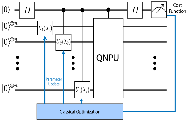
Figure 1: Depiction of variational algorithm for nonlinear quantum dynamics. Here, $H$ is the Hadamard operator, $|{0}\rangle$ ($|{0}\rangle^{\otimes{n}}$) is the single- (multi-) qubit initial state, $U_{i}(\lambda_{i})$ is the unitary operator representing a quantum ansatz that prepares a trial state on the ${i}^{\rm th}$ quantum register, and QNPU is the quantum nonlinear processing unit that evaluates the nonlinear cost function. The value of the cost function is measured from the ancilla qubit and fed into the classical optimizer, which updates the variational parameters of the ansatz until convergence is achieved.

In this article, our objective is twofold. Our first objective is to solve the ground state problem of a one-dimensional, time-independent, nonlinear Schrödinger equation (NLSE) by utilizing the variational quantum computational fluid dynamics (VQCFD) algorithm. We report that real-amplitude ansatz captures the ground state of the problem across various regimes characterized by varying strengths of nonlinearity. Our second objective is to investigate the effects of quantum hardware noise on the performance of the VQCFD algorithm. For this purpose, we first incorporate the quantum noise in simulations to solve for the ground state of the NLSE within the strong nonlinearity regime, for a small system size. We then implement a pre-trained version of the VQCFD algorithm on digital, gate-based superconducting devices. Our findings reveal that quantum hardware noise affects the execution of various blocks within the VQCFD algorithm, leading to discrepancies in the cost function values. We observe a substantial overlap between the trial states constructed in noisy and noiseless settings, demonstrating that the variations in the cost function values arise from the computation processes executed on the variational state. Furthermore, we reveal that despite the discrepancies in the cost function values, the VQCFD algorithm converges to a set of parameters that captures the ground state with over $99\%$ fidelity. Our investigation underscores the adaptability of the VQCFD algorithm in solving complex nonlinear problems, concurrently highlighting the limitations imposed by the quantum hardware noise inherent in the NISQ devices.

The rest of the article is structured as follows: Sec. II introduces the ground state problem of the nonlinear Schrödinger equation (NLSE) and discusses its implementation using the VQCFD algorithm. Sec. III presents numerical results for solving the ground state problem of the NLSE, first in the absence of quantum noise and then in its presence, detailed in Sec. III.1 and Sec. III.2, respectively. Furthermore, Sec. III.3 discusses results obtained from quantum hardware simulations. We summarize in Sec. IV and also present an outlook for future research directions.

II Nonlinear Quantum Dynamics on a Quantum Computer

The nonlinear Schrödinger equation (NLSE) and its variants model various phenomena [24, 25, 26, 27, 28, 29, 30, 31, 32, 33], such as dynamics of light in nonlinear optics [26, 27], envelope solitons and modulation instabilities in plasma physics and surface gravity waves [28], and characteristics including superfluidity and vortex formation in Bose-Einstein Condensates (BEC) [29, 30, 31, 32, 33], to name a few. In dimensionless form, the time-independent NLSE is given as

$$\begin{aligned} \big{[}-\frac{1}{2}\frac{d^{2}}{d{x}^{2}}+V(x)+g{I_{f(x)}}\big{]}{f(x)}=E{f(x)}\;.\end{aligned}$$ (1)

Here, $f(x)$, with $x$ being spatial coordinates, represents a normalized single real-valued function defined over the interval $[a,b]$. The term $I_{f(x)}$ represents the nonlinear interaction, $g$ denotes the strength of the nonlinearity, and $V(x)$ is the external potential. In this study, we consider $I_{f(x)}=|{f(x)}|^{2}$, quadratic potential $V(x)=V_{0}(x-x_{0})^{2}$ centered around $x_{0}=\frac{b-a}{2}$, and periodic boundary conditions such that $f(b)=f(a)$ and $V(b)=V(a)$. It is worth mentioning that small instances of the Eq. (1) can be solved numerically on classical computers by employing imaginary-time evolution [34, 31, 35] or other methods. However, when addressing large instances of nonlinear problems, the limitations associated with memory capacity and computational time inherent in classical computation become increasingly apparent.

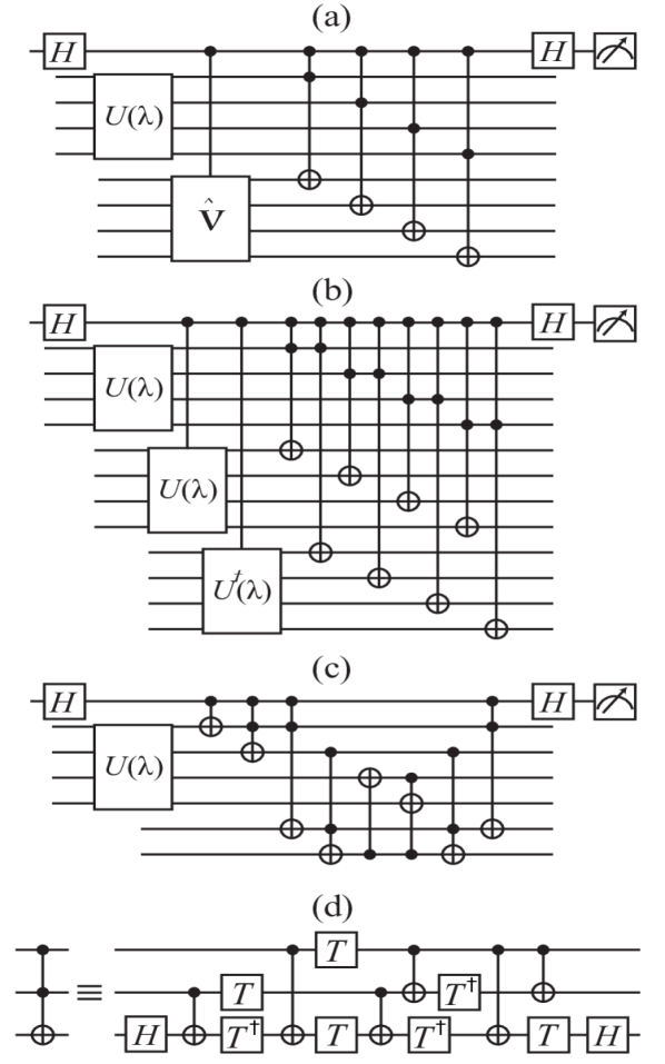
Figure 2: Design of the quantum circuits used to measure the (a) potential, (b) interaction, and (c) kinetic energies. Here, $H$ is the Hadamard gate, $U(\lambda)$ is the quantum ansatz that represents the trial state, and $\hat{V}$ is the potential unitary which encodes the potential function values to the basis states. Here, we have shown an example of $n=4$ ($n^{\prime}=13$), which can be generalized to an arbitrary number of qubits. Panel (d) shows the decomposition of the Toffoli gate into a sequence of single-qubit gates and controlled-NOT gates, where $T=R_{z}(\pi/4)$ and $T^{\dagger}=R_{z}(-\pi/4)$.

Following standard numerical approaches, we discretize the interval $[a,b]$ into $N$ equidistant points $x_{k}=a+\delta{k}$, where $\delta=(b-a)/N$ is the spacing between two adjacent points, and $k\in\{0,1,2,\dots,N-1\}$. The normalization condition on the function $f(x)$ takes the form $1=\delta\sum_{k=0}^{N-1}|{f(x_{k})}|^{2}=\sum_{k=0}^{N-1}|{\psi_{k}}|^{2}$, where we have defined $\psi_{k}=\sqrt{\delta}f(x_{k})$. We encode the $N=2^{n}$ amplitudes $\psi_{k}$, which may also incorporate the initial conditions of the problem, into the basis states $|{\rm binary}(k)\rangle$ of the $n$-qubit quantum register such that the quantum state takes the form $|\Psi\rangle=\sum_{k}\psi_{k}|{\rm binary}(k)\rangle$. By applying the finite-difference method, the expectation value of the total energy [from Eq. (1)] of the system is given as the sum of potential, interaction, and kinetic energies, $\langle\langle{E}\rangle\rangle=\langle\langle{E_{P}}\rangle\rangle+\langle\langle{E_{I}}\rangle\rangle+\langle\langle{E_{K}}\rangle\rangle$, where

$$\begin{aligned} \langle\langle{E_{P}}\rangle\rangle&=\sum_{k=0}^{N-1}~{}|\psi_{k}|^{2}V_{k}\;,~{}~{}~{}~{}\langle\langle{E_{I}}\rangle\rangle=\sum_{k=0}^{N-1}~{}\frac{g}{\delta}|\psi_{k}|^{4}\;,\\ \langle\langle{E_{K}}\rangle\rangle&=-\frac{1}{2\delta^{2}}\sum_{k=0}^{N-1}\big{(}\psi^{\ast}_{k}\psi_{k+1}-2\psi^{\ast}_{k}\psi_{k}+\psi^{\ast}_{k}\psi_{k-1}\big{)}\;,\end{aligned}$$ (2)

for the discretized problem and $\langle\langle{\cdots}\rangle\rangle$ represent the expectation value [22]. We consider the total energy as the cost function $\mathcal{C}=\sum_{j}\mathcal{C}_{j}=\sum_{j}\langle\langle{E_{j}}\rangle\rangle$ for the VQCFD algorithm such that the minimum value of the cost function represents the ground state solution.

In the VQCFD algorithm, each component of the energy cost function is evaluated separately and requires a dedicated quantum nonlinear processing unit (QNPU), as shown in Fig. 2(a-c). For the measurement of potential (interaction) energy, the relevant QNPU constructs the potential function (variational states) on the separate quantum register(s) and performs its (their) bit-wise multiplication with the primary variational state, as depicted in Fig. 2(a) (Fig. 2(b)). The procedure for constructing the unitary operator $\hat{V}$, which represents the potential function, is elaborated in Appendix A. The kinetic energy is calculated using an adder circuit [36, 37, 22] as the QNPU, which requires an additional $n-2$ ancilla qubits, illustrated in Fig. 2(c), where $n$ represents the number of qubits in the primary quantum register. It is important to highlight that performing the Hadamard test and measuring the control qubit in the Pauli-$z$ basis $M$ times allows for an estimation of the cost function value, albeit with a larger variance than direct measurement methods of the $n$-qubit quantum register [38]. This variance stems from the Hadamard test outcomes being either $+1$ or $-1$, contrasting with direct measurements that yield probability densities across $2^{n}$ distinct basis states for more precise cost function estimations. In Sec. III.1, we briefly compare the Hadamard test with direct measurement methods, deferring a detailed analysis to future research.

From Fig. 2(a-c), it is observed that the size of the primary quantum register, $n$, dictating the spatial grid points, $N=2^{n}$, is distinct from the size of the quantum circuit, which also incorporates additional quantum registers and ancilla qubits for evaluating the energy expectation value. For the NLSE problem, the requisite qubit counts for potential, interaction, and kinetic energy calculations are $2n+1$, $3n+1$, and $2n-1$, respectively, necessitating a minimum of $3n+1$ qubits for the cost function evaluation. Throughout this article, we specify the size of the primary quantum register, $n$, and the minimum qubits needed for the evaluation of the cost function, $n^{\prime}$, to elucidate both the scale of the problem and the qubit resources essential for the execution of the VQCFD algorithm.

III Results and Discussion

In this section, we discuss the results of the VQCFD algorithm, where we solve for the ground state of the NLSE (Eq. (1)). First, we consider the noiseless (noisy) settings in Sec. III.1 (III.2) and employ the quantum assembly language (QASM) simulator of the Qiskit [39] platform. Then, we turn our attention to digital, gate-based quantum hardware simulations of pre-trained quantum circuits on superconducting IBM Q devices in Sec. III.3, where we utilize the ibmq-kolkata and ibmq-mumbai devices. Across all simulations, we consider $0.1$ million shots per circuit and adopt the COBYLA optimizer [40, 41, 42]. To prepare the trial state, we consider a real-amplitude ansatz. The ansatz consists of $l$ number of layers where each layer consists of a single-qubit $R_{y}$ gate applied on each qubit followed by a sequence of controlled-NOT (CNOT) gates as depicted in Fig. 3(a). Following the last layer, we apply $R_{y}$ gates to each qubit again such that the ansatz consists of $n(l+1)$ single-qubit gates and variational parameters and $(n-1)l$ CNOT gates. This ansatz transforms the probability amplitudes within the $2^{n}$-dimensional real space of the nonlinear problem.

To benchmark the performance of the VQCFD algorithm, we solve the exact ground state $|\Psi_{\rm GS}\rangle$ (and its energy $\langle\langle{E}\rangle\rangle_{\rm GS}$) of the NLSE using the imaginary time evolution method [34, 31], enabling us to not only gauge the minimum value of the energy cost function but also to calculate state fidelity $F=|\langle\Psi_{\rm GS}|\Psi_{\rm VQCFD}\rangle|^{2}$, which measures how closely the trial state $|\Psi_{\rm VQCFD}\rangle$ resembles the ground state.

III.1 Simulations

As our method is variational and involves probing the total quantum system indirectly, we first test our approach in simulators. This allows us to distinguish the possible deviation from the ideal results originating from the method itself to the one coming from the quantum hardware noise. To analyze the Hadamard test measurement error present in the VQCFD algorithm, we also evaluate the energy expectation value $\langle\langle{E}\rangle\rangle_{\rm Direct}$, which we assume to be exact , using the direct measurement of the n-qubit primary quantum register (see Appendix B for details). It is important to note that while $\langle\langle{E}\rangle\rangle_{\rm Direct}$ is also measured, the classical optimization algorithm exclusively utilizes the $\langle\langle{E}\rangle\rangle_{\rm VQCFD}$ value to update the variational parameters. To this end, we define $\Delta_{r,j}=\langle\langle{E}\rangle\rangle^{r,j}_{\rm VQCFD}-\langle\langle{E}\rangle\rangle^{r,j}_{\rm Direct}$, where $\langle\langle{E}\rangle\rangle^{r,j}_{\rm VQCFD}$ and $\langle\langle{E}\rangle\rangle^{r,j}_{\rm Direct}$ represent the energy expectation values obtained from the Hadamard test and direct measurement methods, respectively, during the $j^{th}$ iteration and $r^{th}$ execution of the VQCFD algorithm. Given that each execution of the VQCFD algorithm is independent of the others, with a different energy value and set of variational parameters, we define the average standard deviation $\sigma=\frac{1}{\sqrt{R{J}}}\sum_{r,j=1}^{R,J}\sqrt{\langle\Delta_{r,j}\rangle_{R,J}-\Delta_{r,j}}$. Here, $\langle\dots\rangle_{R,J}$ denotes the average over the $J$ iterations and $R$ executions of the VQCFD algorithm. The standard deviation, $\sigma$, highlights the average spread of the cost function values, $\langle\langle{E}\rangle\rangle_{\rm VQCFD}$, arising from the Hadamard test measurement error.

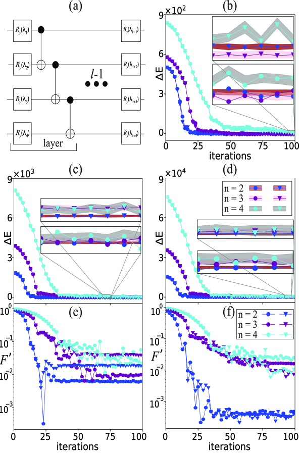
Figure 3: Panel (a) shows the real-amplitude ansatz for the case of $n=4$, where $R_{y}$ is a parameterized single-qubit rotation gate. Energy difference $\Delta{E}=E_{\rm VQCFD}-E_{\rm GS}$ vs iterations of classical optimizer has been shown for (b) weak nonlinearity $g=10$, (c) intermediate value of nonlinearity $g=500$, and (d) strong nonlinearity strength $g=5000$. Trial state infidelity $F^{\prime}=1-|\langle\Psi_{\rm VQCFD}|\Psi_{\rm GS}\rangle|^{2}$, with the ground state, is shown in panel (e) and (f) for $g=500$ and $g=5000$, respectively. Here, blue, purple, and cyan color indicates the qubit numbers $n=2$ ($n^{\prime}=7$), $n=3$ ($n^{\prime}=10$), and $n=4$ ($n^{\prime}=13$) for $l=2$, $l=4$, and $l=7$ layers, respectively. Moreover, circular and triangular markers indicates two different method of executing the VQCFD algorithm (see Sec. III.1 for details).

Figs. 3(b-f) presents the results of noiseless simulations of the VQCFD algorithm. We examine systems comprising $n=2$ ($n^{\prime}=7$), $n=3$ ($n^{\prime}=10$), and $n=4$ ($n^{\prime}=13$) qubits, depicted by blue, purple, and cyan colors, respectively. Circular markers within these figures indicate the best result among $R=20$ executions of the VQCFD algorithm. Additionally, brown, pink, and grey colored regions around the circular markers in Figs. 3(b - d) highlight the range of one standard deviation from the $\langle\langle{E}\rangle\rangle_{\rm Direct}$ values (not shown on the plot).

First, considering a relatively weak nonlinearity strength, $g=10$, circular markers in Fig. 3(b) demonstrate that the VQCFD algorithm converges toward the minimum energy, with the energy difference between the variational energy and the ground state energy approaching zero. Second, for intermediate ($g=500$) and strong ($g=5000$) nonlinearity strengths, circular markers in Fig. 3(c) and 3(d) depict that the VQCFD algorithm converges to the minimum energy. The infidelity ($F^{\prime}=1-F$) between the trial state and the ground state, indicated by circular markers in Figs. 3(e) and 3(f) for $g=500$ and $g=5000$, respectively, highlights that in scenarios of intermediate and strong nonlinearity strengths, the VQCFD algorithm leads to a final trial state with the fidelity exceeding $98\%$. This fidelity may substantially improve by initiating the VQCFD algorithm with an educated guess that possesses a considerable overlap with the ground state. These results highlight that the real-amplitude ansatz efficiently approximates the ground state of the NLSE across different regimes characterized by varying strengths of nonlinearity, thereby demonstrating its expressivity for solving the NLSE with high fidelity.

The insets and circular markers in Figs. 3(b-d) highlight that the range of standard deviation (uncertainty in $\langle\langle{E}\rangle\rangle_{\rm VQCFD}$ due to the Hadamard test measurement) increases with increasing system size. Notably, the energy values (refer to circular markers in insets of Figs. 3(b-d)) obtained from the VQCFD algorithm exhibit fluctuations that may arise for the following reasons: At a given instance of the classical optimization process, the energy cost function value, $\langle\langle{E}\rangle\rangle_{\rm VQCFD}$, which incurs an error due to the Hadamard test measurement, is fed to the classical optimizer and results in an erroneous update of the variational parameters. These updated variational parameters, in turn, lead to an energy value with inherent error, resulting in fluctuating behavior near the minimum value.

To feed a correct or less erroneous value of the energy cost function to the classical optimizer, we average out the Hadamard test measurement error. For this purpose, we consider $R=20$ executions of the quantum circuit at each instance of the classical optimization and obtain an averaged cost function value, $\overline{\langle\langle{E}\rangle\rangle_{\rm VQCFD}}$. This averaged value is then fed to the classical optimizer for the subsequent update of the variational parameters . In Figs. 3(b - d), the triangular markers and colored regions illustrate the difference between the averaged cost function value and the ground state energy, $\overline{\langle\langle{E}\rangle\rangle_{\rm VQCFD}^{j}}-E_{\rm GS}$, and the span of one standard deviation, $\sigma^{\prime}_{j}=\frac{1}{\sqrt{R}}\sum_{r=1}^{R}\sqrt{\overline{\langle\langle{E}\rangle\rangle_{\rm VQCFD}^{j}}-\langle\langle{E}\rangle\rangle_{\rm VQCFD}^{r,j}}$, at $j^{th}$ iteration of the classical optimization. The insets within Figs. 3(b - d) reveal that the process of averaging out the Hadamard test measurement error leads to a smoother convergence toward the ground state energy while maintaining the same level of fidelity between the final trial state and the ground state, as demonstrated in Figs. 3(e - f).

III.2 Simulations Incorporating Superconducting Quantum Hardware Noise

Before we run the circuits on the real quantum hardware, we first implement the algorithm in simulators in the presence of realistic noise (see Appendix C for details). The hardware noise features a mean thermal relaxation time ($T_{1}$) of $100\mu{s}$ and a mean dephasing time ($T_{2}$) of $85\mu{s}$, with standard deviations of $30\mu{s}$ and $50\mu{s}$, respectively. It exhibits mean error rates of $2.625\times 10^{-4}$ for single-qubit gates and $9.616\times 10^{-3}$ for two-qubit gates. Here, we assume trivial qubit reset noise, ensuring that each qubit is perfectly initialized in the $|{0}\rangle$ state at the onset of each computation.

Considering $n=2~{}(n^{\prime}=7)$ qubit system with strong nonlinearity, $g=5000$, triangular (circular) markers in Fig. 4(a) depict the energy expectation in the presence (absence) of quantum noise. It is important to note that only the energy cost function value obtained in the noisy settings is utilized in the classical optimization to update the variational parameters. Fig. 4(a) highlights that although the energy expectation values from the noisy simulations have smaller magnitudes, they exhibit similar behavior to those obtained in the noiseless settings. Furthermore, Fig. 4(b) illustrates that the final trial state in the noisy settings closely matches the ground state, indicating that the noisy simulation converges to the set of variational parameters that approximate the ground state for the problem. The measure of state infidelity $F^{\prime\prime}=1-|\langle\Psi_{\rm VQCFD}^{{}^{\rm{\scriptscriptstyle Noiseless}}}|\Psi_{\rm VQCFD}^{{}^{\rm{\scriptscriptstyle Noisy}}}\rangle|^{2}$ between the trial states generated in noisy and noiseless settings, as depicted in the inset of Fig. 4(b), further suggests that quantum noise scarcely affects the state preparation process within the primary quantum register for system of smaller size.

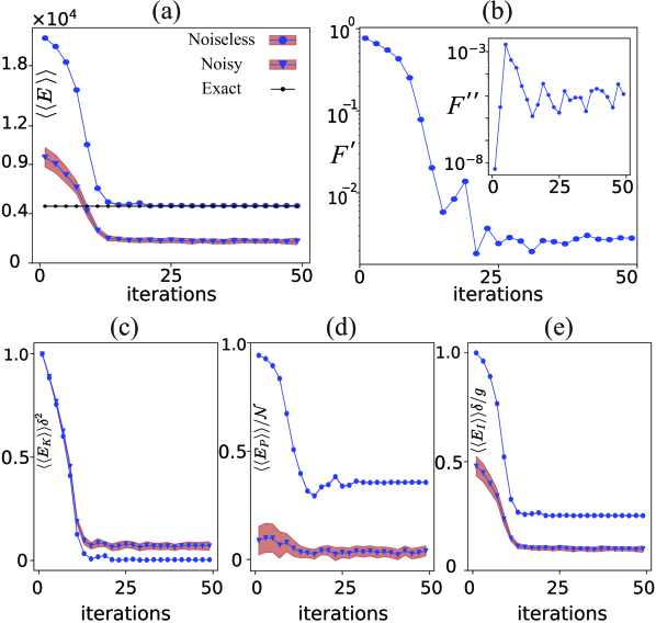
Figure 4: Circular (triangular) markers in panel (a) shows the energy $\langle\langle{E}\rangle\rangle_{\rm VQCFD}$ vs iterations of classical optimizer for $g=5000$, $n=2$ ($n^{\prime}=7$) and $l=2$ of real amplitude ansatz in the absence (presence) of quantum noise. Panel (b) (and the inset therein) shows the infidelity $F^{\prime}=1-|\langle\Psi_{\rm GS}|\Psi^{{}^{\rm Noisy}}_{\rm VQCFD}\rangle|^{2}$ ($F^{\prime\prime}=1-|\langle\Psi^{{}^{\rm Noiseless}}_{\rm VQCFD}|\Psi^{{}^{\rm Noisy}}_{\rm VQCFD}\rangle|^{2}$). Panel (c, d, e) shows the quantities $\langle\langle{E_{K}}\rangle\rangle\delta^{2}$, $\langle\langle{E_{P}}\rangle\rangle/\mathcal{N}$, and $\langle\langle{E_{I}}\rangle\rangle\delta/g$, which are measured from the ancilla qubit during the VQCFD algorithms. Here, $\delta=1/2^{n}$ and $\mathcal{N}$ is the norm of the potential function. Circular (triangular) markers indicates the absence (presence) of quantum noise while brown color highlights the region of one standard deviation.

Given the preparation of a high-fidelity trial state on the primary quantum register, it is pertinent to consider that quantum noise might influence other distinct processes, such as encoding of the potential function, replication of the variational state, and computation of the energy cost function. To analyze the effect of quantum noise, we examine each component individually, noting the difference in outcomes in the presence and absence of quantum noise. First, we assess the kinetic energy component, $\langle\langle{E_{K}}\rangle\rangle/\delta^{2}$, where the corresponding quantum circuit comprises $16$ ($42$) CNOT (single-qubit) quantum gates. As depicted in Fig. 4(c), a minor deviation of approximately $0.05$ is observed in the kinetic energy values. With the trial state already prepared to high fidelity, the observed discrepancy in kinetic energy values could be attributed to the impact of quantum gate noise during the computation process.

Second, we analyze the potential and interaction energy components, $\langle\langle{E_{P}}\rangle\rangle/\mathcal{N}$ and $\langle\langle{E_{I}}\rangle\rangle\delta/g$, with the corresponding quantum circuits incorporating $62$ ($170$) and $133$ ($273$) CNOT (single-qubit) gates, respectively. Notable differences, approximately $0.85$ to $0.35$ and $0.5$ to $0.15$ at the initial and final stages of classical optimization, are observed in Figs. 4(d) and 4(e), reflecting the impact of quantum noise. These disparities in potential and interaction energies likely arise from quantum noise affecting the process of encoding the potential function and replicating the trial states on distinct quantum registers, as well as from the bit-wise multiplication across these registers. For instance, noise impacting the encoding (replication) of the potential function $\hat{V}$ (variational state $|\Psi_{\rm VQCFD}\rangle$) could result in an entirely different potential function $\hat{V}\pm\hat{\delta{V}}$ (variational state $|\Psi^{\prime}_{\rm VQCFD}\rangle$). Consequently, these discrepancies result in the potential, interaction, and total energy dropping below the minimum levels for the given system. Our investigation reveals that deeper quantum circuits with a substantial number of imperfect CNOT and single-qubit gates result in significant deviation and variance in the cost function values, emphasizing the necessity for advanced noise mitigation and/or error correction strategies to improve the quantum computational accuracy and reliability of the VQCFD algorithm.

III.3 Implementation on Superconducting Cloud Hardware

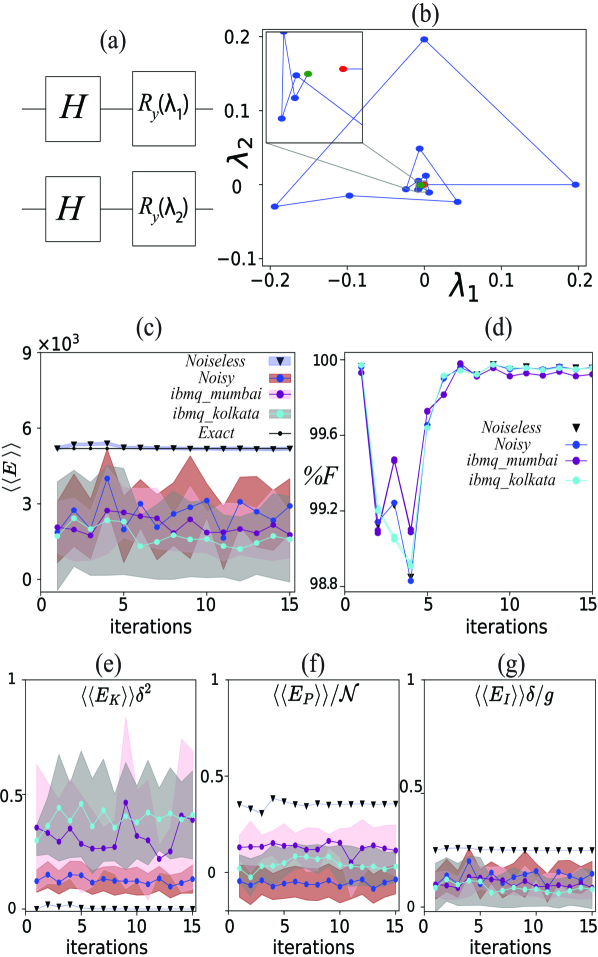
Figure 5: Panel (a) shows the simplified quantum ansatz adopted for the quantum device demonstration of the VQCFD algorithm. Panel (b) represent the training of variational parameters, where red (green) marker highlight the initial (final) point of the classical optimization. Panel (c) shows the energy $\langle\langle{E}\rangle\rangle_{\rm VQCFD}$ vs iterations of classical optimizer for $g=5000$, $n=2$ ($n^{\prime}=7$). Here, blue (black) color indicate the noisy (noiseless) simulations, while purple and cyan colors represent simulations performed on ibmq-mumbai and ibmq-kolkata devices, respectively. Moreover, the blue, brown, pink, and gray colors highlight the region of one standard deviation. Panel (d) shows the fidelity $\%F=|\langle\Psi_{\rm GS}|\Psi_{\rm VQCFD}\rangle|^{2}\times{100}$ of the trial state with respect to the ground state solution. Panel (e, f, g) shows the quantities $\langle\langle{E_{K}}\rangle\rangle\delta^{2}$, $\langle\langle{E_{P}}\rangle\rangle/\mathcal{N}$, and $\langle\langle{E_{I}}\rangle\rangle\delta/g$, and corresponding standard deviations.

We now implement a pre-trained VQCFD algorithm on the digital gate-based quantum devices, ibmq-kolkata and ibmq-mumbai [45]. Despite both devices featuring identical topology and basis gate set, the selection of these two devices is motivated by the differences in their single and two-qubit error rates. We focus on an $n=2$ ($n^{\prime}=7$) qubit system with $g=5000$ and design the quantum ansatz tailored to the strong nonlinearity case, such that each qubit has a Hadamard gate followed by a parameterized single-qubit $R_{y}$ rotation gate, as shown in Fig. 5(a). This simplified ansatz offers two advantages. The first advantage is the absence of controlled-NOT gates, resulting in quantum circuits with fewer entangling gates and a shallow circuit depth. Consequently, the quantum circuits to measure kinetic, potential, and interaction energies consist of $14$, $59$, and $70$ ($33$, $160$, and $124$) CNOT (single-qubit) gates, respectively. The second advantage is that, for the zero value of each variational parameter, the quantum ansatz generates a uniform trial state with over $99\%$ fidelity with the exact ground state in the strong nonlinearity regime. This insight allows us to restrict the variational space closer to the ground state, such that even for the non-zero but smaller values of the variational parameters, the trial state maintains considerable overlap with the ground state. With this setting, we train the quantum ansatz in the presence of quantum noise, where each variational parameter is initiated at a zero value (red point in Fig. 5(b)). The classical optimizer explores the two-dimensional variational space for a few iterations before converging toward the zero values of the variational parameters (a green point in Fig. 5(b) indicates the set of final values of the variational parameters).

With the pre-trained variational parameters, we measure the energy cost function and trial state fidelity in both noiseless simulations and noisy settings of simulations and digital quantum hardware. It is worth noting that, unlike the noisy simulations, quantum hardware simulations exhibit qubit reset noise. Fig. 5(d) demonstrates the fidelity of the trial state with a maximum disparity of $0.25\%$ between noiseless simulations and quantum device simulations, highlighting the high-fidelity preparation of the trial state across the two devices. Additionally, the evaluation of the energy cost function in both noiseless (depicted in black) and noisy (depicted in blue) simulations, as shown in Figs. 5(c), 5(e-g), aligns with the findings presented in Sec. III.2, with differences and variances stemming from the impact of quantum noise.

Figs. 5(c) and 5(e-g) show the energy cost function and individual components measured on the ibmq-mumbai (in purple color) and ibmq-kolkata (in cyan color) devices. The results exhibit behavior akin to those observed in the noisy simulations. Here, the qubit reset noise, causing imperfect initialization of ancilla qubits and quantum registers, further impacts the encoding (preparation) of the potential function (variational state) and the execution of the adder circuit, resulting in significant increases in standard deviation values. These findings reveal large errors and variances, thereby highlighting the limitations of the current NISQ devices in executing the VQCFD algorithm.

IV Summary and Outlook

In this work, we studied the ground state problem of the nonlinear Schrödinger equation by utilizing the variational quantum computational fluid dynamics (VQCFD) algorithm. For a quadratic potential, we demonstrated that the real-amplitude ansatz, which spans the $2^{n}$-dimensional real space of the problem, has the expressivity to represent the ground state in the weak, intermediate, and strong regimes of nonlinearity. Furthermore, we analyzed the Hadamard test measurement error against a direct method and observed that the Hadamard test measurement error results in fluctuations in the cost function, potentially leading to optimization challenges. These fluctuations in the cost function can be averaged out by repeated measurements of the same quantum circuit, thus providing a more stable and reliable basis for the optimization process.

Secondly, we incorporated quantum hardware noise into the simulations and reported that while the VQCFD algorithm produces a high-fidelity ground state for the small system, the values of the cost function and its constituting components are significantly influenced by hardware noise. We argued that, given the high-fidelity trial state, quantum noise affects the cost function computation during the execution of the quantum nonlinear processing unit (QNPU). Finally, we implemented pre-trained circuits on the ibmq-kolkata and ibmq-mumbai devices and observed that qubit reset noise, which was not considered in the noisy simulations, further affects the evaluation of the cost function. Our results highlight the limitations of the current NISQ devices for the implementation of the VQCFD algorithm.

In the future, an extensive analysis of the Hadamard test measurement error might be an interesting aspect to pursue, especially where it is critical to explore how the Hadamard test measurement error scales with the number of qubits, depth of the quantum circuit, and the number of entangling gates. Furthermore, studying noise mitigation and error correction techniques to improve the cost function evaluation in the VQCFD algorithm would be intriguing. Lastly, the investigation of fluid dynamics problems, modeled by the one-dimensional Burgers’ equation and the two- and three-dimensional Navier-Stokes equations, is worthwhile, where a few key aspects to analyze may include the expressivity of various ansatzes, challenges of classical optimization, and the impact of quantum noise, to name a few.

Appendix A Construction of Potential Unitary

In this section, we discuss the encoding of the potential function into a unitary matrix $\hat{V}$ such that $V_{k}=\mathcal{N}\langle{\rm binary}(k)|\hat{V}|{0}\rangle=\mathcal{N}\langle{\rm binary}(k)|{\psi_{P}}\rangle$, where $\mathcal{N}$ is the norm of the potential function, $|{\rm binary}(k)\rangle$ is the $k^{th}$ basis state, and

$$\begin{aligned} |\psi_{P}\rangle=\hat{V}|{0}\rangle=\sum_{i_{1},\dots,i_{n}}V_{i_{1},\dots,i_{n}}|i_{1},\dots,i_{n}\rangle\end{aligned}$$

is the state that we intend to prepare on a separate quantum register (refer to Fig. 2(a)). Here, $|i_{1},\dots,i_{n}\rangle=|{\rm binary}(k)\rangle$ are the $n$-qubit basis states, $V_{i_{1},\dots,i_{n}}=V_{k}/\mathcal{N}$ are the potential values or probability amplitudes of the state, and $i^{\prime}$s are the physical indices representing qubits. For this purpose, we utilize the framework of matrix product states (MPS) [46, 47, 48, 49] and transform the state $|{\psi_{P}}\rangle$ in the form

$$\begin{aligned} |\psi_{P}\rangle=\sum_{i_{1},\dots,i_{n}}A_{i_{1},r_{1}}A_{r_{1},i_{2},r_{2}}\dots&~{}{A_{r_{n-2},i_{n-1},r_{n-1}}}\\ &~{}~{}~{}~{}~{}~{}~{}~{}A_{r_{n-1},i_{n}}|i_{1},\dots,i_{n}\rangle,\end{aligned}$$ (3)

where the first and last tensors are of rank-$2$, the middle tensors are of rank-$3$, and $r^{\prime}$s represent dummy indices that control the bond-dimension of the matrix product states [48, 49]. Here, we have considered the Einstein summation convention where repeated indices are summed over. Moreover, without loss of generality, we consider each ($i$) $r$ to be (two-) $2^{j}$-dimensional for $j\in\{1,2,\dots,n-1\}$.

Given a high-rank tensor $V_{i_{1},\dots,i_{n}}$, we perform successive operations: reshaping, where a high-rank tensor is reshaped into a rank-$2$ tensor; singular value decomposition (SVD) $M=\mathcal{S}\mathcal{V}\mathcal{D}^{T}$, where a rank-$2$ tensor is decomposed into matrices of singular values and corresponding right and left eigenvectors; and tensor contraction, where two or more tensors are contracted to form a single tensor. Here, singular values of matrix $M$ are arranged in descending order in the diagonal of the $\mathcal{V}$-matrix, and left (right) eigenvectors of $M$ form the columns of matrix $\mathcal{S}$ ($\mathcal{D}$). The general algorithm to obtain the MPS format of Eq. (3) is as follows.

1 Input: High rank tensor;

2 while Number of tensors $<$ Number of qubits do

3       Reshape tensor into matrix: $V_{i_{1},\dots,i_{n}}\rightarrow M_{i_{1},i_{2}\dots i_{n}}$ ;

4       Perform SVD decomposition of matrix: $M=\mathcal{S}\mathcal{V}\mathcal{D}^{T}$ ;

5       Contract $\mathcal{V}$ and $\mathcal{D}^{T}$: $M^{{}^{\prime}}=\mathcal{V}\mathcal{D}^{T}$ ;

6       Update: $V=M^{{}^{\prime}}$ ;

7      

8Reshape isometries to appropriate rank ;

return MPS Format.

Algorithm 1 MPS Algorithm

With a maximum value of bond dimension $\nu=2^{\kappa}$, the MPS in the left canonical form is written as

$$\begin{aligned} &V_{i_{1},\dots,i_{n}}\\ &~{}~{}~{}~{}=\sum_{\begin{subarray}{c}r_{j}=1\\ j=1,\dots,n-1\end{subarray}}^{D}{A}_{i_{1},r_{1}}{A}_{r_{1},i_{2},r_{2}}\dots&{A}_{r_{n-2},i_{n-1},r_{n-1}}{A}_{r_{n-1},i_{n}}\end{aligned}$$

where,

$$D=\left\{\begin{array}[]{ll}2^{j},&~{}~{}~{}if~{}~{}~{}2^{j}\leq\nu\\ \nu,&~{}~{}~{}if~{}~{}~{}2^{j}>\nu.\end{array}\right.$$ (6)

Here, $\nu=2^{\kappa}$ determines the accuracy of the approximation of the matrix product states (MPS) and bond dimensions between adjacent tensors are $2,2^{2},...,2^{\kappa-1},2^{\kappa},...,2^{\kappa},2^{\kappa-1},...,2^{2},2$. The contraction of two adjacent tensors with a common bond dimension of $2^{j}$ is represented by $j$ overlapping qubits between the two unitary gates, as shown in Fig. 6(a).

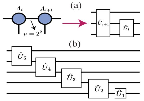
Figure 6: Panel (a) illustrates the transformation of a small tensor network into a unitary circuit, highlighting that the bond dimension of $2^{j}$ between two adjacent tensors results in $j$ overlapping qubits for the two unitary gates. Schematic of a quantum circuit obtained from a tensor network with a maximum bond dimension of $2$ is shown in panel (b).

To transform the MPS format into unitary gates, we follow the procedure described in Ref. [22]. For the given MPS format, we first contract all the leftmost tensors up to the bond dimension $2^{\kappa-1}$. The MPS representation then comprises of $n-(\log_{2}(v)-1)$ tensors with bond dimensions ranging from $2^{\kappa}$ to $2$, between adjacent tensors. Given the compact MPS representation, each tensor contains fewer elements, which are insufficient for creating the appropriate gates. To address this issue, we extend each tensor by combining it with its nullspace and adding an additional index, thus compensating for the missing elements needed for the suitable gate. Each middle tensor is transformed into a rank-$4$, while the leftmost and rightmost tensors are transformed into rank-$3$ tensors. Finally, we reshape each extended tensor into a matrix, carefully maintaining the qubit ordering. The placement of each element within the unitary is critical, as it corresponds to different qubits in the quantum circuit. A generic algorithm for transforming the MPS format into a quantum circuit is as follows.

1 Input: MPS format;

2 Contract tensors up to bond dimension $2^{\kappa-1}$;

3 for each remaining tensor do

4       Reshape rank-$3$ tensor into matrix: $A_{r_{j-1},i_{j},r_{j}}\xrightarrow{}M_{r_{j-1}i_{j},r_{j}}$ ;

5       Stack the tensor with its nullspace by introducing an extra index ;

6       Reshape the extended tensor into a matrix ;

7       Rearrange indices according to qubit ordering convention ;

8      

9Apply resulting unitaries to a quantum circuit ;

10 return Quantum Circuit;

Algorithm 2 MPS to Quantum Circuit

An example of a quantum circuit representing a generic MPS of bond dimension $2$ is shown in Fig. 6(b).

Appendix B Direct measurement of cost function

In this section, we describe a direct measurement method of evaluating the cost function discussed in Ref. [22], which does not involve a quantum nonlinear processing unit (QNPU), ancilla qubits, and the Hadamard test measurement. We use this direct measurement method to validate the cost function evaluation of the VQCFD algorithm.

We consider an $n$-qubit quantum register such that it describes the nonlinear problem on $N=2^{n}$ grid points. This quantum register is initialized in the fixed $|{0}\rangle^{\otimes{n}}$ state. The initial state is then transformed into some final state by applying the quantum ansatz $U(\lambda)$ considered in the VQCFD algorithm. As the final step, we measure all the qubits, as shown in Fig. 7(a), and obtain the probability outcome $|\psi_{k}|^{2}$ associated with each basis state $|{\rm binary}(k)\rangle$. The probability density is then plugged into Eq. (2) to compute the expectation values of potential energy $\langle\langle{E_{P}}\rangle\rangle=\sum_{k}|\psi_{k}|^{2}V_{k}$ and interaction energy $\langle\langle{E_{I}}\rangle\rangle=\sum_{k}|\psi_{k}|^{m+2}$ on a classical computer.

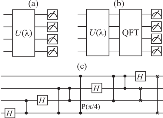
Figure 7: Panel (a) depicts the quantum circuit to calculate the probability density of the final state. This probability density is used to calculate the expectation value of potential and interaction energies. Panel (b) depicts the quantum circuit used to construct the quantum state $|\Psi^{\prime}\rangle={\rm QFT}|\Psi\rangle$ in the basis of the Laplace operator. Measuring all the qubits give probability density $|\psi^{\prime}_{k}|^{2}$. Panel (c) shows the decomposition of the quantum Fourier transform operation, where $H$ is the Hadamard gate and $P(\pi/4)$ is the controlled-phase gate.

To evaluate the expectation value of kinetic energy, we transform the final state using a quantum Fourier transform (QFT) circuit [35], which also diagonalizes the Laplace operator. This way we represent the final state in the basis of the Laplace operator. The expectation value of kinetic energy is then given as $\langle\langle{E_{K}}\rangle\rangle=\frac{1}{2}\langle\psi|{\rm(QFT)}^{\dagger}\hat{D}_{\Delta}{\rm(QFT)}|\psi\rangle=\frac{1}{2}\sum_{k}|\psi^{{}^{\prime}}_{k}|^{2}\Delta_{k}$, where $\hat{D}_{\Delta}$ has $\Delta_{k}$ values along the diagonal, and $\Delta_{k}=2^{2n}\big{[}\cos(2\pi{k}/2^{n})-1\big{]}$ are the eigenvalues of the Laplace operator. Here, $|\psi^{{}^{\prime}}_{k}|^{2}$ is the probability of the $k^{th}$ basis state obtained by measuring all the qubits after applying quantum Fourier transform to the final state as depicted in Fig. 7(b-c). We obtain the expectation value of total energy by summing up individual components $\langle\langle{E_{Direct}}\rangle\rangle=\langle\langle{E_{P}}\rangle\rangle+\langle\langle{E_{I}}\rangle\rangle+\langle\langle{E_{K}}\rangle\rangle$. Here, $\langle\langle{E_{Direct}}\rangle\rangle$ is the energy expectation value obtained using the direct method, as discussed above. In the absence of any noise, direct measurement method gives the correct expectation values of kinetic, potential, and interaction energies.

Appendix C Noisy Simulator

Various types of noise errors have been identified that detrimentally impact the computational performance of quantum hardware. These sources encompass reset errors, wherein the qubit is initialized in an imperfect state; measurement errors, wherein the qubit’s state (either $|{0}\rangle$ or $|{1}\rangle$) is inaccurately measured ($|{1}\rangle$ or $|{0}\rangle$, respectively); and gate errors, wherein interactions with the environment induce irregularities in the outcomes of quantum operations.

To model the effect of quantum hardware noise within our simulations, we prepare a noisy quantum assembly language (QASM) simulator tailored to the noise properties of the ibmq-kolkata device and execute the simulations on this noisy QASM simulator. The device properties include relaxation and coherence times ($T_{1}$ and $T_{2}$) for each qubit, gate duration ($\tau$) for each single- and two-qubit gate, and probabilities $P_{01}$ ($P_{10}$) of measuring state $|{0}\rangle$ ($|{1}\rangle$) when the qubit is prepared in state $|{1}\rangle$ ($|{0}\rangle$). Given that the device calibration data does not contain any information on the qubit reset error, we neglect the effect of this error in the noisy simulations. Subsequently, we utilize the calibration data within Qiskit’s integrated functions to configure a noisy QASM simulator. Moreover, we incorporate the device’s coupling map and transpile each quantum circuit to the basis gate set of the ibmq-kolkata device. This methodology yields an approximate noise model, albeit one that does not encapsulate all potential sources of noise errors inherent to the quantum devices. In the noisy simulations presented in this work, we utilized the ibmq-kolkata device calibration data obtained at $05:37$ GMT on November $28$, $2023$.

References

- Shor [1994] P. W. Shor, Proceedings 35th Annual Symposium on Foundations of Computer Science , 124 (1994).
- Grover [1996] L. K. Grover, Proceedings of the 28th annual ACM symposium on Theory of computing , 212 (1996).
- Harrow et al. [2009] A. W. Harrow, A. Hassidim, and S. Lloyd, Phys. Rev. Lett. 103, 150502 (2009).
- Abrams and Lloyd [1997] D. S. Abrams and S. Lloyd, Phys. Rev. Lett. 79, 2586 (1997).
- Abrams and Lloyd [1999] D. S. Abrams and S. Lloyd, Phys. Rev. Lett. 83, 5162 (1999).
- Cerezo et al. [2021] M. Cerezo, A. Arrasmith, R. Babbush, S. C. Benjamin, S. Endo, K. Fujii, J. R. McClean, K. Mitarai, X. Yuan, L. Cincio, et al., Nature Reviews Physics 3, 625 (2021).
- Bharti et al. [2022] K. Bharti, A. Cervera-Lierta, T. H. Kyaw, T. Haug, S. Alperin-Lea, A. Anand, M. Degroote, H. Heimonen, J. S. Kottmann, T. Menke, W.-K. Mok, S. Sim, L.-C. Kwek, and A. Aspuru-Guzik, Rev. Mod. Phys. 94, 015004 (2022).
- Peruzzo et al. [2014] A. Peruzzo, J. McClean, P. Shadbolt, M.-H. Yung, X.-Q. Zhou, P. J. Love, A. Aspuru-Guzik, and J. L. O’brien, Nature communications 5, 4213 (2014).
- Kandala et al. [2017] A. Kandala, A. Mezzacapo, K. Temme, M. Takita, M. Brink, J. M. Chow, and J. M. Gambetta, Nature 549, 242 (2017).
- McClean et al. [2016] J. R. McClean, J. Romero, R. Babbush, and A. Aspuru-Guzik, New Journal of Physics 18, 023023 (2016).
- O’Malley et al. [2016] P. J. J. O’Malley, R. Babbush, I. D. Kivlichan, J. Romero, J. R. McClean, R. Barends, J. Kelly, P. Roushan, A. Tranter, N. Ding, B. Campbell, Y. Chen, Z. Chen, B. Chiaro, A. Dunsworth, A. G. Fowler, E. Jeffrey, E. Lucero, A. Megrant, J. Y. Mutus, M. Neeley, C. Neill, C. Quintana, D. Sank, A. Vainsencher, J. Wenner, T. C. White, P. V. Coveney, P. J. Love, H. Neven, A. Aspuru-Guzik, and J. M. Martinis, Phys. Rev. X 6, 031007 (2016).
- Hempel et al. [2018] C. Hempel, C. Maier, J. Romero, J. McClean, T. Monz, H. Shen, P. Jurcevic, B. P. Lanyon, P. Love, R. Babbush, A. Aspuru-Guzik, R. Blatt, and C. F. Roos, Phys. Rev. X 8, 031022 (2018).
- Ganzhorn et al. [2019] M. Ganzhorn, D. Egger, P. Barkoutsos, P. Ollitrault, G. Salis, N. Moll, M. Roth, A. Fuhrer, P. Mueller, S. Woerner, I. Tavernelli, and S. Filipp, Phys. Rev. Appl. 11, 044092 (2019).
- Quantum et al. [2020] G. A. Quantum, Collaborators*†, F. Arute, K. Arya, R. Babbush, D. Bacon, J. C. Bardin, R. Barends, S. Boixo, M. Broughton, B. B. Buckley, et al., Science 369, 1084 (2020).
- Farhi et al. [2014] E. Farhi, J. Goldstone, and S. Gutmann, arXiv preprint arXiv:1411.4028 https://doi.org/10.48550/arXiv.1411.4028 (2014), https://arxiv.org/abs/1411.4028 .
- Pagano et al. [2020] G. Pagano, A. Bapat, P. Becker, K. S. Collins, A. De, P. W. Hess, H. B. Kaplan, A. Kyprianidis, W. L. Tan, C. Baldwin, et al., Proceedings of the National Academy of Sciences 117, 25396 (2020).
- Tan et al. [2021] B. Tan, M.-A. Lemonde, S. Thanasilp, J. Tangpanitanon, and D. G. Angelakis, Quantum 5, 454 (2021).
- Zhu et al. [2022] L. Zhu, H. L. Tang, G. S. Barron, F. A. Calderon-Vargas, N. J. Mayhall, E. Barnes, and S. E. Economou, Phys. Rev. Res. 4, 033029 (2022).
- Benedetti et al. [2019] M. Benedetti, E. Lloyd, S. Sack, and M. Fiorentini, Quantum Science and Technology 4, 043001 (2019).
- Zhu et al. [2019] D. Zhu, N. M. Linke, M. Benedetti, K. A. Landsman, N. H. Nguyen, C. H. Alderete, A. Perdomo-Ortiz, N. Korda, A. Garfoot, C. Brecque, et al., Science advances 5, eaaw9918 (2019).
- Tangpanitanon et al. [2020] J. Tangpanitanon, S. Thanasilp, N. Dangniam, M.-A. Lemonde, and D. G. Angelakis, Phys. Rev. Res. 2, 043364 (2020).
- Lubasch et al. [2020] M. Lubasch, J. Joo, P. Moinier, M. Kiffner, and D. Jaksch, Physical Review A 101, 010301 (2020).
- Jaksch et al. [2023] D. Jaksch, P. Givi, A. J. Daley, and T. Rung, AIAA journal 61, 1885 (2023).
- Scott [2006] A. Scott, Encyclopedia of nonlinear science (Routledge, New York, 2006).
- Agrawal [2013] G. Agrawal, Nonlinear fiber optics. (2013).
- Nakkeeran [2002] K. Nakkeeran, Chaos, Solitons & Fractals 13, 673 (2002).
- Triki et al. [2019] H. Triki, C. Bensalem, A. Biswas, S. Khan, Q. Zhou, S. Adesanya, S. P. Moshokoa, and M. Belic, Optics Communications 437, 392 (2019).
- Sulem and Sulem [1999] C. Sulem and P.-L. Sulem, The nonlinear schrödinger equation: self-focusing and wave collapse (Springer Science & Business Media, 1999).
- Gross [1961] E. P. Gross, Il Nuovo Cimento (1955-1965) 20, 454 (1961).
- Pitaevskii [1961] L. P. Pitaevskii, Sov. Phys. JETP 13, 451 (1961).
- Dalfovo et al. [1999] F. Dalfovo, S. Giorgini, L. P. Pitaevskii, and S. Stringari, Reviews of modern physics 71, 463 (1999).
- Leggett [2001] A. J. Leggett, Reviews of modern physics 73, 307 (2001).
- Pitaevskii and Stringari [2003] L. Pitaevskii and S. Stringari, Bose-Einstein condensation (2003).
- Edwards and Burnett [1995] M. Edwards and K. Burnett, Physical Review A 51, 1382 (1995).
- Lubasch et al. [2018] M. Lubasch, P. Moinier, and D. Jaksch, Journal of Computational Physics 372, 587 (2018).
- Vedral et al. [1996] V. Vedral, A. Barenco, and A. Ekert, Physical Review A 54, 147 (1996).
- Nielsen and Chuang [2010] M. A. Nielsen and I. L. Chuang, Quantum computation and quantum information (Cambridge University Press, 2010).
- Polla et al. [2023] S. Polla, G.-L. R. Anselmetti, and T. E. O’Brien, Phys. Rev. A 108, 012403 (2023).
- Anis et al. [2021] M. S. Anis, H. Abraham, R. A. AduOffei, G. Agliardi, M. Aharoni, I. Y. Akhalwaya, G. Aleksandrowicz, T. Alexander, M. Amy, S. Anagolum, et al., Qiskit/qiskit 10.5281/zenodo.2573505 (2021).
- Powell [1994] M. J. Powell, A direct search optimization method that models the objective and constraint functions by linear interpolation (Springer, 1994).
- Powell [1998] M. J. Powell, Acta numerica 7, 287 (1998).
- Powell [2007] M. J. Powell, Mathematics Today-Bulletin of the Institute of Mathematics and its Applications 43, 170 (2007).
- Note [1] Direct measurement does not involve the QNPU and ancilla qubits. Direct measurement of quantum registers has small statistical errors due to shot noise. This error decreases as we increase the number of shots. In our case, we consider to be exact, given the large number of shots - million. Therefore, we do not analyze the statistical error in the energy values obtained from the direct measurement method.
- Note [2] We execute the VQCFD algorithm in two distinct ways. In the first method, we implement the VQCFD algorithm times with the same set of initial parameters. It is worth noting that each execution differs, given the randomness of the classical optimization procedure. We then choose the best result out of executions. In the second method, we execute each quantum circuit times for a given set of variational parameters and obtain the cost function value as the average of these executions. We then feed this average value of the cost function to the classical optimizer and update the variational parameters for the next iteration.
- [45] IBM Quantum, https://quantum.ibm.com/, 2021.
- Verstraete et al. [2008] F. Verstraete, V. Murg, and J. I. Cirac, Advances in physics 57, 143 (2008).
- Oseledets [2013] I. V. Oseledets, Constructive Approximation 37, 1 (2013).
- Orús [2014] R. Orús, Annals of physics 349, 117 (2014).
- Cirac et al. [2021] J. I. Cirac, D. Pérez-García, N. Schuch, and F. Verstraete, Rev. Mod. Phys. 93, 045003 (2021).