Optimal testing in a class of nonregular models

Abstract.

This paper studies optimal hypothesis testing for nonregular statistical models with parameter-dependent support. We consider both one-sided and two-sided hypothesis testing and develop asymptotically uniformly most powerful tests based on the likelihood ratio process. The proposed one-sided test involves randomization to achieve asymptotic size control, some tuning constant to avoid discontinuities in the limiting likelihood ratio process, and a user-specified alternative hypothetical value to achieve the asymptotic optimality. Our two-sided test becomes asymptotically uniformly most powerful without imposing further restrictions such as unbiasedness. Simulation results illustrate desirable power properties of the proposed tests.

1. Introduction

This paper studies optimal hypothesis testing of a class of nonregular statistical models in which the boundary of the support of the observed data depends on some parameter of interest. Such nonregular models have been often applied in the statistics literature, and typically imply discontinuous likelihood functions and nonstandard convergence rates of estimators. Classic examples include Ibragimov and Hasminskii, (1981, Chapter V) who conducted an asymptotic analysis on univariate densities with jumps at an end point of parameter-dependent support, and Cheng and Amin, (1983) and Smith, (1985) who studied properties of the maximum likelihood estimator of parametric models with shifted origins. In contrast to most existing papers, this paper focuses on optimal (composite) hypothesis testing for nonregular models instead of point estimation.

For testing a simple null hypothesis against a simple alternative one, Neyman-Pearson’s fundamental lemma yields an optimal power property of the likelihood ratio test even for the case of parameter-dependent support. However, such an optimality result is not available for general testing problems, such as one-sided testing. On the other hand, for regular statistical models, it is known that standard testing methods (such as the likelihood ratio, Wald, and score tests) can achieve certain asymptotic optimal power properties for testing general composite hypotheses (see, Chapter 15 of Lehmann and Romano,, 2022). An open question is whether we can establish an analogous asymptotic optimality result for testing composite hypotheses on nonregular parameters in the case of parameter-dependent support.

In a special case where the monotone likelihood ratio condition holds, the uniformly most powerful one-sided test can be typically constructed by the minimum (or maximum) of the sample. However, this condition is violated for many cases including (parameter-dependent) truncated versions of the normal, t, Laplace, and logistic distributions. Moreover, if the model contains conditioning variables, the conventional theory based on the monotone likelihood ratio condition is typically not applicable.

In this paper, we consider one-sided and two-sided hypothesis testing for parametric models with parameter-dependent support and develop an asymptotically uniformly most powerful (AUMP) test based on the likelihood ratio process, called the nonregular likelihood ratio (NLR) test. Our construction of the one-sided test involves (i) certain randomization to achieve asymptotic size control, (ii) a tuning constant to avoid discontinuous points of the limiting likelihood ratio process, and (iii) an alternative hypothetical value to evaluate the likelihood ratio, which needs to be chosen to achieve the optimality. Moreover, we construct a two-sided NLR test that attains the AUMP property without imposing further restrictions such as unbiasedness. Our two-sided NLR test does not have randomization, and can be inverted to construct a confidence set for the nonregular parameter. For clarity we first present the main results under a benchmark setup in Section 2, where there is no nuisance parameter. Then we extend our optimality results for the NLR test to a general setup in Section 3 that involves nuisance parameters and covariates. For the general case, we need some independent auxiliary sample to estimate the nuisance parameters, which is typically obtained by sample splitting. Our simulation results in Section 4 illustrate desirable power properties of the proposed NLR test.

In addition to the papers cited above, Hirano and Porter, (2003) studied efficient point estimation of parameter-dependent support models by extending the limits of experiments argument, and showed that the Bayes estimator is asymptotically efficient under a minimax criterion but the maximum likelihood estimator is generally inefficient. To the best of our knowledge, this paper is the first one that studies optimal hypothesis testing for nonregular models with parameter-dependent support. In contrast to the Bayes estimator in Hirano and Porter, (2003) that involves priors on parameters, our optimal testing methods are developed as modifications of likelihood ratio statistics associated with randomization and a tuning constant to deal with discontinuities in the likelihood ratio. Chernozhukov and Hong, (2004) also investigated nonstandard asymptotic properties of estimation and testing methods for parameter-dependent support models. They established asymptotic optimality of the Bayes estimators in terms of the asymptotic average risk, and showed that the Wald test and Bayes posterior quantiles are valid for inference. However, they did not discuss optimality of the testing methods. In our simulation study, we demonstrate that the proposed NLR test exhibits higher power than the Wald type test by Chernozhukov and Hong, (2004). Severini, (2004) studied higher-order approximations for the likelihood ratio statistics of parameter-dependent support models. Fan et al., (2000) derived the asymptotic distribution of the likelihood ratio statistic for some nonregular models whose asymptotic distribution follows a gamma distribution. Lin et al., (2019) generalized the notion of the Fisher information to non-regular problems.

2. Benchmark case

This section presents our main results for a simple nonregular model with a scalar parameter and no covariate. This model, covering the uniform distribution as a canonical example, provides a useful benchmark to highlight our developments. We propose one-sided tests for this model and derive several asymptotic properties of these tests, including asymptotic uniform power optimality.

Let $Y\in\mathcal{Y}\subset\mathbb{R}$ follow the parametric model

$$Y\sim f(y|\theta)\mathbb{I}\{y\geq g(\theta)\},$$ (1)

where $\mathbb{I}\{\cdot\}$ is the indicator function, $\theta\in\Theta\subset\mathbb{R}$ is the true value of a scalar parameter, and conditions on the functions $f$ and $g$ are specified below. For this model, we consider the one-sided testing problem

$$H_{0}:\theta=\theta_{0}\quad\text{against}\quad H_{1}^{+}:\theta>\theta_{0}\text{ (or }H_{1}^{-}:\theta<\theta_{0}\text{)},$$ (2)

for a given $\theta_{0}\in\Theta$. Hereafter we focus on the case of $\nabla_{\theta}g(\theta_{0})>0$. The case of $\nabla_{\theta}g(\theta_{0})<0$ is analyzed in the same manner. Based on the reparametrization $h=n(\theta-\theta_{0})$, this testing problem is written as

$$H_{0}:h=0\quad\text{against}\quad H_{1}^{+}:h>0,\text{ (or }H_{1}^{-}:h<0\text{)}.$$ (3)

We wish to test $H_{0}$ based on an independent and identically distributed (iid) sample $Y^{n}=(Y_{1},\ldots,Y_{n})$ of $Y$. Although our results can be easily extended to cover a more general reparametrization $h=n(\theta-\theta_{0})+\zeta_{n}$ with $\zeta_{n}=o(1)$, we focus on the case of $\zeta_{n}=0$ for simplicity.

Our testing procedure is constructed based on the likelihood ratio process. Since the joint density of $Y^{n}$ is written as

$$\mathrm{d}P_{\theta}^{n}(y^{n})=\mathbb{I}\{y_{(1)}\geq g(\theta)\}\prod_{i=1}^{n}f(y_{i}|\theta),$$

where $y_{(1)}=\min\{y_{1},\ldots,y_{n}\}$, the likelihood ratio process on a parameter space $\mathcal{H}\subseteq\mathbb{R}$ is

$$Z_{n}(h,\bar{h}):=\frac{\mathrm{d}P_{\theta_{0}+\frac{\bar{h}}{n}}^{n}}{\mathrm{d}P_{\theta_{0}+\frac{h}{n}}^{n}}(Y^{n})=\frac{\mathbb{I}\{Y_{(1)}\geq g(\theta_{0}+\bar{h}/n)\}}{\mathbb{I}\{Y_{(1)}\geq g(\theta_{0}+h/n)\}}\prod_{i=1}^{n}\frac{f(Y_{i}|\theta_{0}+\bar{h}/n)}{f(Y_{i}|\theta_{0}+h/n)},$$

for $h,\bar{h}\in\mathcal{H}$. To characterize asymptotic properties of this process, we impose the following assumptions.

Assumption 1.

   

(i):

$\{Y_{i}\}_{i=1}^{n}$ is an iid sample of $Y\in\mathcal{Y}\subset\mathbb{R}$ with the Lebesgue density in (1). The parameter space $\Theta$ is convex.

(ii):

$f(y|\theta)$ is twice continuously differentiable in $\theta$ for all $y$. In some open neighborhood $\mathcal{N}$ of $\theta_{0}$, $f(y|\theta)$ and $\nabla_{\theta}f(y|\theta)$ are continuous in $y$ for $\theta\in\mathcal{N}$, there exists a constant $C$ such that $0<f(y|\theta)<C<\infty$ for all $y$ and $\theta\in\mathcal{N}$, and

$$\int\sup_{\theta\in\mathcal{N}}\left\|\nabla_{\theta}f(y|\theta)\right\|\mathbb{I}\{y\geq g(\theta)\}dy<\infty,$$

$$\int\sup_{\theta,\bar{\theta}\in\mathcal{N}}\frac{\left\|\nabla_{\theta}f(y|\bar{\theta})\right\|^{2}}{f(y|\bar{\theta})^{2}}\mathbb{I}\{y\geq g(\theta)\}f(y|\theta)dy<\infty,$$

$$\int\sup_{\theta,\bar{\theta}\in\mathcal{N}}\frac{\left\|\nabla_{\theta\theta}f(y|\bar{\theta})\right\|}{f(y|\bar{\theta})}\mathbb{I}\{y\geq g(\theta)\}f(y|\theta)dy<\infty.$$

$g(\theta)$ is continuously differentiable in $\theta$, $\nabla_{\theta}g(\theta_{0})>0$, and $\sup_{\theta\in\mathcal{N}}\left\|\nabla_{\theta}g(\theta)\right\|<\infty$.

Assumption 1 (i) is standard, and Assumption 1 (ii) contains smoothness and boundedness conditions on the functions $f$ and $g$ in (1). By adapting Hirano and Porter, (2003, Theorem 2) to our setup, Assumption 1 guarantees weak convergence (denoted by “$\rightsquigarrow$”) of the likelihood ratio process

$$\{Z_{n}(h,\bar{h})\}_{\bar{h}\in I}\rightsquigarrow\{Z(h,\bar{h})\}_{\bar{h}\in I}:=\{e^{(\bar{h}-h)/\lambda}D_{h,\bar{h}}\}_{\bar{h}\in I}\quad\text{under }P_{\theta_{0}+\frac{h}{n}},$$ (4)

for every finite $I\subset\mathcal{H}$, where $\lambda=\{f(g(\theta_{0})|\theta_{0})\nabla_{\theta}g(\theta_{0})\}^{-1}$ and

$$D_{h,\bar{h}}:=\mathbb{I}\{W_{h}>\bar{h}\}\text{ with }W_{h}\sim f_{W}(w|h)=\frac{1}{\lambda}e^{-(w-h)/\lambda}\mathbb{I}\{w>h\}.$$

Note that $\lambda$ is a known constant in the present setup. In contrast to the standard likelihood ratio process, which is locally asymptotically normal, $Z_{n}(h,\bar{h})$ converges to a limit of experiment whose randomness is given by the binary variable $D_{h,\bar{h}}$. This is due to lack of differentiability in quadratic mean of the density $\mathrm{d}P_{\theta}^{n}(y^{n})$. Since $D_{h,\bar{h}}$ is discrete, the limiting likelihood ratio process $Z(h,\bar{h})$ is discontinuous in the sense that $\Pr\{Z(h,\bar{h})\leq z\}$ is not continuous at $z=0$ and $e^{(\bar{h}-h)/\lambda}$. Thus, we cannot use the conventional asymptotic theory to evaluate asymptotic size and power properties of testing procedures for $H_{0}$.

To overcome this difficulty, we propose the nonregular likelihood ratio (NLR) test that shifts the rejection cutoff slightly above the discontinuous point. In particular, our testing procedure for $H_{0}:h=0$ against $H_{1}^{+}:h>0$ (or $H_{1}^{-}:h<0$) is constructed by using the likelihood ratio statistic $Z_{n}(0,\bar{h})$ combined with a suitably chosen $\bar{h}$ to achieve a certain power optimality and rejection rule for controlling its asymptotic size. Hereafter we separately consider testing against the alternatives $H_{1}^{+}:h>0$ (Section 2.1) and $H_{1}^{-}:h<0$ (Section 2.2). Based on the one-sided tests, we also propose a two-sided test against the alternative $H_{1}:h\neq 0$ (Section 2.3).

2.1. Test against $H_{1}^{+}:h>0$

We first consider testing $H_{0}:h=0$ against $H_{1}^{+}:h>0$. In this case, we choose some $\bar{h}>0$. Given the significance level $\alpha\in(0,1)$, our NLR test is defined as

$$\phi_{n}(Y^{n}|\bar{h},\varepsilon)=\left\{\begin{array}[]{lll}1&\text{if}&Z_{n}(0,\bar{h})>e^{\bar{h}/\lambda}(1+\varepsilon)\text{ or }Y_{(1)}<g(\theta_{0})\\ \alpha e^{\bar{h}/\lambda}&\text{if}&Z_{n}(0,\bar{h})\in[e^{\bar{h}/\lambda}(1-\varepsilon),e^{\bar{h}/\lambda}(1+\varepsilon)]\\ 0&\text{if}&Z_{n}(0,\bar{h})<e^{\bar{h}/\lambda}(1-\varepsilon)\end{array}\right.,$$ (5)

for $\alpha\leq e^{-\bar{h}/\lambda}$ with some $\varepsilon\in(0,1)$, and

$$\phi_{n}(Y^{n}|\bar{h},\varepsilon)=\left\{\begin{array}[]{lll}1&\text{if}&Z_{n}(0,\bar{h})>e^{\bar{h}/\lambda}\varepsilon\text{ or }Y_{(1)}<g(\theta_{0})\\ \frac{\alpha-e^{-\bar{h}/\lambda}}{1-e^{-\bar{h}/\lambda}}&\text{if}&Z_{n}(0,\bar{h})\in[-e^{\bar{h}/\lambda}\varepsilon,e^{\bar{h}/\lambda}\varepsilon]\\ 0&\text{if}&Z_{n}(0,\bar{h})<-e^{\bar{h}/\lambda}\varepsilon\end{array}\right.,$$ (6)

for $\alpha>e^{-\bar{h}/\lambda}$ with some $\varepsilon\in(0,e^{-\bar{h}/\lambda})$ (see Remark 3 below for the choice of $\varepsilon$). Here $\phi_{n}(Y^{n}|\bar{h},\varepsilon)=1$ and $0$ mean rejection and acceptance of $H_{0}$, respectively. When $Y_{(1)}<g(\theta_{0})$, the likelihood ratio $Z_{n}(0,\bar{h})$ is indeterminant, and we reject $H_{0}$ by convention.

Remark 1.

There are three key features of the construction of the NLR test. First, the test is constructed for two categories, $\alpha\leq e^{-\bar{h}/\lambda}$ and $\alpha>e^{-\bar{h}/\lambda}$. This categorization comes from the Neyman-Pearson test for the limiting one sample problem; see Remark 2. Second, the NLR test involves randomization. Applied researchers who dislike the randomization results can simply report the randomization probability instead of “flipping coin” to reject or accept. Third, the NLR test requires a tuning constant $\varepsilon$, which is introduced to avoid discontinuous points of the limiting likelihood ratio process $Z(h,\bar{h})$. Our simulation results in the supplement (Section B) also confirm the importance of non-zero $\varepsilon$. See Remark 3 below for a practical choice of $\varepsilon$.

Let $E_{\theta}[\cdot]$ be the expectation under $P_{\theta}^{n}$. The asymptotic properties of the NLR test are obtained as follows.

Lemma 1.

Suppose that Assumption 1 holds true with the (unknown) true local parameter value $h\geq 0$. Then the NLR test in (5) and (6) with a user specified value $\bar{h}>0$ satisfies the following:

(i):

It is of asymptotic level $\alpha$ (i.e., $\limsup_{n}E_{\theta_{0}}[\phi_{n}(Y^{n}|\bar{h},\varepsilon)]\leq\alpha$).

(ii):

Its asymptotic local power satisfies $\lim\inf_{n}E_{\theta_{0}+h/n}[\phi_{n}(Y^{n}|\bar{h},\varepsilon)]\geq\pi_{L}(h,\bar{h})$ for $h>0$, where

$$\pi_{L}(h,\bar{h}):=\left\{\begin{array}[]{ll}\alpha e^{\min\{h,\bar{h}\}/\lambda}&\text{for }\alpha\leq e^{-\bar{h}/\lambda}\\ \frac{\alpha-e^{-\bar{h}/\lambda}}{1-e^{-\bar{h}/\lambda}}+\min\{e^{(h-\bar{h})/\lambda},1\}\frac{1-\alpha}{1-e^{-\bar{h}/\lambda}}&\text{for }\alpha>e^{-\bar{h}/\lambda}\end{array}\right..$$ (7)

(iii):

$\Pi(\bar{h}):=\pi_{L}(\bar{h},\bar{h})$ attains power of the Neyman-Pearson test for testing $H_{0}^{W}:W\sim f_{W}(w|0)$ against $H_{1}^{W}:W\sim f_{W}(w|\bar{h})$. Moreover,

$$\Pi(h)=\begin{cases}\alpha e^{h/\lambda}&\text{for }\alpha\leq e^{-h/\lambda}\\ 1&\text{for }\alpha>e^{-h/\lambda}\end{cases}$$

satisfies $\Pi(h)\geq\pi_{L}(h,\bar{h})$ for any $h,\bar{h}>0$.

Remark 2.

In the limiting one sample test for $W$ (i.e., $H_{0}^{W}$ against $H_{1}^{W}$ in (iii)), the Neyman-Pearson test is constructed as

$$\phi(W)=\begin{cases}\left\{\begin{array}[]{lll}1&\text{if}&Z(\bar{h},\bar{h})>e^{\bar{h}/\lambda}Z(\bar{h},0)\\ \alpha e^{\bar{h}/\lambda}&\text{if}&Z(\bar{h},\bar{h})=e^{\bar{h}/\lambda}Z(\bar{h},0)\\ 0&\text{if}&Z(\bar{h},\bar{h})<e^{\bar{h}/\lambda}Z(\bar{h},0)\end{array}\right.&\text{for }\alpha\leq e^{-\bar{h}/\lambda}\\ \left\{\begin{array}[]{lll}1&\text{if}&Z(\bar{h},\bar{h})>0\\ \frac{\alpha-e^{-\bar{h}/\lambda}}{1-e^{-\bar{h}/\lambda}}&\text{if}&Z(\bar{h},\bar{h})=0\\ 0&\text{if}&Z(\bar{h},\bar{h})<0\end{array}\right.&\text{for }\alpha>e^{-\bar{h}/\lambda}\end{cases}.$$

The NLR test in (5) and (6) is a (smoothed) sample counterpart of this Neyman-Pearson test.

Note that Lemma 1 contains three local parameter values: the null hypothetical value $0$, fixed alternative value $\bar{h}$ chosen by users, and true local parameter value $h$ generating the data. Lemma 1 (i) says that the NLR test achieves asymptotic size control, and Lemma 1 (ii) characterizes a lower bound for the asymptotic local power of the NLR test. Furthermore, Lemma 1 (iii) says that the NLR test is tangent to the power envelope at $h=\bar{h}$. We note that the value $\alpha e^{\min\{h,\bar{h}\}/\lambda}$ in (7) originates in the randomization. Thus, randomization is essential even in the Neyman-Pearson test for $H_{0}^{W}$ against $H_{1}^{W}$ because of the discreteness of the limiting likelihood ratio.

To implement the NLR test, we need to choose $\bar{h}$. To this end, we invert the envelope power function $\Pi(h)$ with a fixed level $\alpha$. This approach is also used in Elliott et al., (1996) for unit root testing. For the case of $\alpha\leq e^{-\bar{h}/\lambda}$, Lemma 1 (iii) suggests that $\bar{h}$ may be chosen to satisfy $\pi=\Pi(\bar{h})$ for a specified value of $\pi$, that is

$$\bar{h}^{+}(\pi)=\lambda\log\left(\frac{\pi}{\alpha}\right).$$

Indeed if we set $\pi=1$ (i.e., $\bar{h}^{+}:=\bar{h}^{+}(1)=-\lambda\log\alpha$), then the NLR test $\phi_{n}(Y^{n}|\bar{h}^{+},\varepsilon)$ achieves an asymptotic optimal property in Definition 1 below, introduced by Choi et al., (1996). Since we can choose $\bar{h}$ to satisfy $\alpha\leq e^{-\bar{h}/\lambda}$, we can ignore the case of $\alpha>e^{-\bar{h}/\lambda}$. Indeed, our simulation in the supplement (Section B) suggests that the power decreases for large $\bar{h}$ with $\alpha>e^{-\bar{h}/\lambda}$.

Definition 1 (Asymptotically uniformly most powerful test).

For testing $H_{0}:\theta=\theta_{0}$ against $H_{1}:\theta>\theta_{0}$ (or $\theta<\theta_{0}$ or $\theta\neq\theta_{0}$), a sequence of tests $\{\phi_{n}\}$ is called asymptotically uniformly most powerful (AUMP) in $\mathcal{H}$ at asymptotic level $\alpha$ if $\limsup_{n}E_{\theta_{0}}[\phi_{n}]\leq\alpha$ and for any other sequence of test functions $\{\psi_{n}\}$ satisfying $\limsup_{n}E_{\theta_{0}}[\psi_{n}]\leq\alpha$,

$$\liminf_{n}E_{\theta_{0}+h/n}[\phi_{n}]\geq\limsup_{n}E_{\theta_{0}+h/n}[\psi_{n}],$$

for every $h>0$ (or $h<0$ or $h\neq 0$) in $\mathcal{H}$.

Theorem 1.

Suppose that Assumption 1 holds true with the true local parameter $h\geq 0$. The NLR test $\phi_{n}(Y^{n}|\bar{h}^{+},\varepsilon)$ is AUMP in $\mathcal{H}$ at level $\alpha$ for testing $H_{0}:\theta=\theta_{0}$ against $H_{1}^{+}:\theta>\theta_{0}$.

Based on Lemma 1 (ii) and (iii), we know that the NLR test is asymptotically most powerful test when $h=\bar{h}$, i.e., the true local parameter equals to what we choose. However, this choice is infeasible since $h$ is unknown. Theorem 1 says that if we choose $\bar{h}$ carefully (i.e., $\bar{h}=\bar{h}^{+}$), the NLR test becomes asymptotically uniformly most powerful.

The choice $\bar{h}=\bar{h}^{+}$ is reasonable since $\bar{h}^{+}$ attains the maximum of the power envelope function. The simple reason why this choice is AUMP is that $\bar{h}=\bar{h}^{+}$ is at the end point of the region $\alpha\leq e^{-\bar{h}/\lambda}$. For the case $\alpha\leq e^{-\bar{h}/\lambda}$, the NLR test rejects on the region $[e^{\bar{h}/\lambda}(1+\varepsilon),\infty)$ and randomly reject with probability $\alpha e^{\bar{h}/\lambda}$ on the region $[e^{\bar{h}/\lambda}(1-\varepsilon),e^{\bar{h}/\lambda}(1+\varepsilon)]$. The choice $\bar{h}=\bar{h}^{+}$ maximizes the rejection region since we reject with probability $\alpha e^{\bar{h}^{+}/\lambda}=1$ on the randomization region, i.e., the randomization region becomes the rejection region. Hence, $\bar{h}=\bar{h}^{+}$ should attain the power envelope as long as true data generating process occurs by $h$ with $e^{-\bar{h}^{+}/\lambda}=\alpha\leq e^{-h/\lambda}$. Moreover, when true data generating process occurs by $h$ with $e^{-\bar{h}^{+}/\lambda}=\alpha>e^{-h/\lambda}$, i.e. $h>\bar{h}^{+}$, it is easier to reject $H_{0}:h=0$ since the true parameter $h$ is grater than the fixed local alternative $\bar{h}^{+}$. Indeed, the power curve is saturated at $h=\bar{h}^{+}$ and equals to one.

Remark 3 (Choice of $\varepsilon$).

Theorem 1 holds true for any $\varepsilon\in(0,1)$. If we choose $\bar{h}=\bar{h}^{+}$, the NLR test in (5) does not involve randomization and the rejection region gets larger as $\varepsilon$ approaches to $1$. On the other hand, if we choose $\bar{h}\neq\bar{h}^{+}$, then there is no such a clear conclusion for the choice of $\varepsilon$ due to presence of randomization. However, our simulation in the supplement (Section B) suggests that the power increases as $\varepsilon$ approaches to 1 for (5) or approaches to 0 for (6).

2.2. Test against $H_{1}^{-}:h<0$

We now consider testing $H_{0}:h=0$ against $H_{1}^{-}:h<0$. The basic idea is same as the previous case. In this case, we choose some $\bar{h}<0$ and significance level $\alpha\in(0,1)$. We consider the following test:

$$\phi_{n}(Y^{n}|\bar{h},\varepsilon)=\left\{\begin{array}[]{lll}1&\text{if}&Z_{n}(0,\bar{h})>e^{\bar{h}/\lambda}(1+\varepsilon)\text{ or }Y_{(1)}<g(\theta_{0})\\ \alpha&\text{if}&Z_{n}(0,\bar{h})\in[e^{\bar{h}/\lambda}(1-\varepsilon),e^{\bar{h}/\lambda}(1+\varepsilon)]\\ 0&\text{if}&Z_{n}(0,\bar{h})<e^{\bar{h}/\lambda}(1-\varepsilon)\end{array}\right.,$$ (8)

where $\varepsilon\in(0,1)$ is a constant (see Section 4 below for its choice). When $Y_{(1)}<g(\theta_{0})$, we reject $H_{0}$. In contrast to the previous subsection, the test is not categorized by the value of $\alpha$ since the Neyman-Pearson test for the limiting one sample test (i.e, $H_{0}^{W}$ against $H_{1}^{W}$ in Lemma 2 (iii)) does not depend on the value of $\bar{h}$. Thus, it will essentially be a simpler problem than the one in the previous subsection. In this case, the asymptotic properties of $\phi_{n}(Y^{n}|\bar{h},\varepsilon)$ are obtained as follows.

Lemma 2.

Suppose that Assumption 1 holds true with the true local parameter $h\leq 0$. Then the test $\phi_{n}(Y^{n}|\bar{h},\varepsilon)$ with $\bar{h}<0$ and $\varepsilon\in(0,1)$ satisfies the following:

(i):

It is of asymptotic level $\alpha$ (i.e., $\limsup_{n}E_{\theta_{0}}[\phi_{n}(Y^{n}|\bar{h},\varepsilon)]\leq\alpha$),

(ii):

Its asymptotic local power, $\lim\inf_{n}E_{\theta_{0}+h/n}[\phi_{n}(Y^{n}|\bar{h},\varepsilon)]$, is at least

$$\pi_{L}(h,\bar{h})=\min\{e^{(h-\bar{h})/\lambda},1\}-(1-\alpha)e^{h/\lambda},$$

(iii):

$\Pi(\bar{h})=\pi_{L}(\bar{h},\bar{h})$ attains power of the Neyman-Pearson test for testing $H_{0}^{W}:W\sim f_{W}(w|0)$ against $H_{1}^{W}:W\sim f_{W}(w|\bar{h})$. Moreover, $\Pi(h)=1-(1-\alpha)e^{h/\lambda}$ satisfies $\Pi(h)\geq\pi_{L}(h,\bar{h})$ for any $h,\bar{h}>0$.

Similar comments to Lemma 1 apply. Lemma 2 (iii) suggests that $\bar{h}$ may be chosen to satisfy $\pi=\Pi(\bar{h})$ for a specified value of $\pi$, that is

$$\bar{h}^{-}(\pi)=\lambda\log\left(\frac{1-\pi}{1-\alpha}\right).$$

A default choice is $\pi=1$, which gives $\bar{h}^{-}(1)=-\infty$. However, weak convergence and the previous lemma do not cover the local alternative $\bar{h}=-\infty$. Thus, for the test against $H_{1}^{-}:h<0$ we will restrict the local parameter space $\mathcal{H}$ as $\mathcal{H}\subset[-M,+\infty)$, where $M$ is an arbitrary large constant. We denote $\bar{h}^{-}:=-M$, and consider the NLR test $\phi_{n}(Y^{n}|\bar{h}^{-},\varepsilon)$ for $H_{1}^{-}$. Similar to Theorem 1, asymptotic optimality of this test is obtained as follows.

Theorem 2.

Suppose that Assumption 1 holds true with the true local parameter $h\leq 0$. The NLR test $\phi_{n}(Y^{n}|\bar{h}^{-},\varepsilon)$ for any $\varepsilon\in(0,1)$ is AUMP in $\mathcal{H}\subset[-M,+\infty)$ at level $\alpha$ for testing $H_{0}:\theta=\theta_{0}$ against $H_{1}^{-}:\theta<\theta_{0}$.

Remark 4 (Choice of $\varepsilon$).

Theorem 2 holds true for any $\varepsilon\in(0,1)$. In practice, we can use $\bar{h}=-\infty$. If we choose $\bar{h}=-\infty$, the NLR test in (8) does not involve the tuning constant $\varepsilon$ nor randomization. Our simulation in Section 4 also suggests that the power is insensitive to the choice of $\varepsilon$ when we set sufficiently small negative numbers for $\bar{h}$.

2.3. Two-sided test

For two-sided testing

$$H_{0}:h=0\quad\text{against}\quad H_{1}:h\in[-M,0)\cup(0,+\infty),$$

we propose a test function $\phi_{n}(Y^{n}|\bar{h}^{+},\bar{h}^{-},\varepsilon):=\min\{1,\phi_{n}(Y^{n}|\bar{h}^{+},\varepsilon)+\phi_{n}(Y^{n}|\bar{h}^{-},\varepsilon)\}$ with $\bar{h}^{+}=-\lambda\log\alpha$ and $\bar{h}^{-}=-M$, where we combine $\phi_{n}(Y^{n}|\bar{h}^{+},\varepsilon)$ with level $\alpha$ and $\phi_{n}(Y^{n}|\bar{h}^{-},\varepsilon)$ with level $0$. That is,

$$\phi_{n}(Y^{n}|\bar{h}^{+},\bar{h}^{-},\varepsilon)$$ (11)

$$= \left\{\begin{array}[]{lll}1&\text{if}&Z_{n}(0,\bar{h}^{+})\geq e^{\bar{h}^{+}/\lambda}(1-\varepsilon)\text{ or }Z_{n}(0,\bar{h}^{-})>e^{\bar{h}^{-}/\lambda}(1+\varepsilon)\text{ or }Y_{(1)}<g(\theta_{0})\\ 0&\text{if}&Z_{n}(0,\bar{h}^{+})<e^{\bar{h}^{+}/\lambda}(1-\varepsilon)\text{ and }Z_{n}(0,\bar{h}^{-})\leq e^{\bar{h}^{-}/\lambda}(1+\varepsilon)\end{array}\right.,$$

with some $\varepsilon\in(0,1)$. Note that (11) does not include a randomized rejection area because $\phi_{n}(Y^{n}|\bar{h}^{+},\varepsilon)$ and $\phi_{n}(Y^{n}|\bar{h}^{-},\varepsilon)$ with level $0$ do not randomize. The next theorem shows that this test is AUMP.

Theorem 3.

Suppose that Assumption 1 holds true with the true local parameter $h\in\mathcal{H}$. The NLR test $\phi_{n}(Y^{n}|\bar{h}^{+},\bar{h}^{-},\varepsilon)$ for any $\varepsilon\in(0,1)$ is AUMP in $\mathcal{H}\subset[-M,+\infty)$ at level $\alpha$ for testing $H_{0}:\theta=\theta_{0}$ against $H_{1}:\theta\neq\theta_{0}$.

Remark 5.

Importantly, the proposed test attains an AUMP property without imposing any restrictions such as unbiasedness. Also, the weightings for two sides are unequal, in the sense that we assign level $\alpha$ for $h>0$ and level $0$ for $h<0$. These two features are shared by a finite sample UMP two-sided test for the uniform distributions $U(0,\theta)$ (e.g., Lehmann and Romano,, 2022, Problem 3.2, p.105).

Remark 6 (Confidence set).

Since the two-sided test does not randomize, we can easily construct a $(1-\alpha)$% confidence set by test inversion:

$$CS=\{\theta\in\Theta:Z_{n}^{\theta}(0,\bar{h}^{+})<e^{\bar{h}^{+}/\lambda}(1-\varepsilon)\text{ and }Z_{n}^{\theta}(0,\bar{h}^{-})\leq e^{\bar{h}^{-}/\lambda}(1+\varepsilon)\},$$

where

$$Z_{n}^{\theta}(0,\bar{h}):=\frac{\mathbb{I}\{Y_{(1)}\geq g(\theta+\bar{h}/n)\}}{\mathbb{I}\{Y_{(1)}\geq g(\theta)\}}\prod_{i=1}^{n}\frac{f(Y_{i}|\theta+\bar{h}/n)}{f(Y_{i}|\theta)}.$$

This confidence set also has a pointwise optimal property (asymptotically uniformly most accurate) by the same reasoning as in the finite sample case.

3. General case

In this section, we generalize the parametric model to contain discrete covariates and nuisance parameters:

$$Y|X=x\sim f(y|x,\theta,\gamma)\mathbb{I}\{y\geq g(x,\theta)\},$$ (12)

where $\theta\in\Theta\subset\mathbb{R}$ is a scalar parameter of interest, $\gamma\in\mathbb{R}^{d}$ is a vector of (regular) nuisance parameters, $Y$ is a scalar dependent variable, and $X$ is an $m$-dimensional vector of discrete covariates with support $\mathcal{X}=\{a_{1},\dots,a_{L}\}$. This section considers the one-sided testing problem

$$H_{0}:\theta=\theta_{0},\gamma\in\mathbb{R}^{d}\quad\text{against}\quad H_{1}^{+}:\theta>\theta_{0},\gamma\in\mathbb{R}^{d}\text{ (or }H_{1}^{-}:\theta<\theta_{0},\gamma\in\mathbb{R}^{d}\text{)},$$

for a given $\theta_{0}\in\mathbb{R}$ with the asymptotic level of significance $\alpha$. By reparametrization $h=n(\theta-\theta_{0})$, this testing problem is written as

$$H_{0}:h=0,\gamma\in\mathbb{R}^{d}\quad\text{against}\quad H_{1}^{+}:h>0,\gamma\in\mathbb{R}^{d}\text{ (or }H_{1}^{-}:h<0,\gamma\in\mathbb{R}^{d}\text{)}.$$

Let $(Y^{n},X^{n})=((Y_{1},\ldots,Y_{n}),(X_{1},\ldots,X_{n}))$ be an iid sample of $(Y,X)\in\mathbb{R}\times\mathcal{X}$. To extend our benchmark results in the last section, we consider the plug-in likelihood ratio process

$$Z_{n}(h,\check{h}_{n},\check{\gamma}_{n}):=\prod_{i=1}^{n}\frac{f(Y_{i}|X_{i},\theta_{0}+\check{h}_{n}/n,\check{\gamma}_{n})\mathbb{I}\{Y_{i}\geq g(X_{i},\theta_{0}+\check{h}_{n}/n)\}}{f(Y_{i}|X_{i},\theta_{0}+h/n,\check{\gamma}_{n})\mathbb{I}\{Y_{i}\geq g(X_{i},\theta_{0}+h/n)\}},$$ (13)

for $h\in\mathcal{H}$ with a parameter space $\mathcal{H}\subseteq\mathbb{R}$, where $\check{\gamma}_{n}$ and $\check{h}_{n}$ are some estimators of the nuisance parameters $\gamma$ and the user-specified alternative value $\bar{h}$, respectively, based on auxiliary data independent from the main sample $(Y^{n},X^{n})$. In contrast to the benchmark case, optimal values of $\bar{h}$ for the NLR test will depend on some population objects which need to be estimated (see Theorems 4 and 5 below). Thus we introduce an estimator $\check{h}_{n}$ for $\bar{h}$ in this general case. Typically we split the sample (say, $(Y^{2n},X^{2n})$) into the main sample $(Y^{n},X^{n})$ and auxiliary one $((Y_{n+1},\ldots,Y_{2n}),(X_{n+1},\ldots,X_{2n}))$ to obtain $\check{\gamma}_{n}$ and $\check{h}_{n}$.

In this section, we impose the following assumptions.

Assumption 2.

   

(i):

$\{Y_{i},X_{i}\}_{i=1}^{n}$ is an iid sample of $\mathcal{Y}\times\mathcal{X}$, where $\mathcal{Y}\subset\mathbb{R}$ and $\mathcal{X}=\{a_{1},\dots,a_{L}\}$ with the conditional density in (12). The parameter space $\Theta\times\Gamma$ of $(\theta,\gamma)$ is convex.

(ii):

$\{\check{h}_{n}\}$ is a random sequence independent from $(Y^{n},X^{n})$ satisfying $\sqrt{n}(\check{h}_{n}-\bar{h})=O_{P_{\theta_{0}+\frac{h}{n},\gamma}}(1)$ for some user specified constant $\bar{h}$. $\{\check{\gamma}_{n}\}$ is a random sequence independent from $(Y^{n},X^{n})$ satisfying $\sqrt{n}(\check{\gamma}_{n}-\gamma)=O_{P_{\theta_{0}+\frac{h}{n},\gamma}}(1)$.

(iii):

Let $\beta=(\theta,\gamma^{\prime})^{\prime}$ and $\beta_{0}=(\theta_{0},\gamma^{\prime})^{\prime}$. $f(y|x,\beta)$ is twice continuously differentiable in $\beta$ for all $y$ and $x$, and $g(x,\theta)$ is continuously differentiable in $\theta$ for all $x$. In some open neighborhood $\mathcal{N}$ of $\beta_{0}$, $f(y|x,\beta)$ and $\nabla_{\beta}f(y|x,\beta)$ are continuous in $y$ for $\beta\in\mathcal{N}$, there exists a constant $C$ such that $0<f(y|x,\beta)<C<\infty$ for all $y$, $x$, and $\beta\in\mathcal{N}$, and for each $j=1,\ldots,L$,

$$\int\sup_{\beta\in\mathcal{N}}\left\|\nabla_{\beta}f(y\mid a_{j},\beta)\right\|\mathbb{I}\{y\geq g(a_{j},\theta)\}dy<\infty,$$

$$\int\sup_{\bar{\beta},\beta\in\mathcal{N}}\frac{\left\|\nabla_{\beta}f(y\mid a_{j},\bar{\beta})\right\|^{2}}{f(y\mid a_{j},\bar{\beta})^{2}}\mathbb{I}\{y\geq g(a_{j},\theta)\}f(y\mid a_{j},\beta)dy<\infty,$$

$$\int\sup_{\bar{\beta},\beta\in\mathcal{N}}\frac{\left\|\nabla_{\beta\beta}f(y\mid a_{j},\bar{\beta})\right\|}{f(y\mid a_{j},\bar{\beta})}\mathbb{I}\{y\geq g(a_{j},\theta)\}f(y\mid a_{j},\beta)dy<\infty.$$

$\nabla_{\theta}g(a_{j},\theta_{0})>0$, $\sup_{\beta\in\mathcal{N}}\left\|\nabla_{\theta}g(a_{j},\theta)\right\|<\infty$, and $\Pr\{X=a_{j}\}>0$ for each $j=1,\ldots,L$.

As specified in Assumption 2 (i), we focus on the case where covariates are discrete variables. Assumption 2 (ii) requires that the nuisance parameters $\gamma$ and the alternative value $\bar{h}$ to construct our NLR statistics below can be estimated at the $\sqrt{n}$ rate. For example, based on an auxiliary sample independent from $(Y^{n},X^{n})$, $\gamma$ can be estimated by the maximum likelihood and $\bar{h}$ can be estimated by the method of moments. This assumption enables us to focus on a neighborhood to establish the weak convergence in Lemma 3 below. Since $\check{h}_{n}$ and $\gamma_{n}$ are independent from the main sample $(Y^{n},X^{n})$, we can argue the weak convergence in a straightforward way even after conditioning on the concentration to the neighborhood. Assumption 2 (iii) lists boundedness and smoothness conditions on the functions $f$ and $g$.

To present the limiting distribution of the plug-in likelihood ratio process $\{Z_{n}(h,\check{h}_{n},\check{\gamma}_{n})\}$, we introduce further notations. Let

$$\lambda = E_{X}[f(g(X,\theta_{0})|X,\beta_{0})\nabla_{\theta}g(X,\theta_{0})]^{-1},$$

$$D_{h,\bar{h}} = \mathrm{Bernoulli}(\exp(-E_{X}[\mathbb{I}\{\bar{h}-h\geq 0\}f(g(X,\theta_{0})|X,\beta_{0})\nabla_{\theta}g(X,\theta_{0})(\bar{h}-h)])),$$

$G_{j}=\nabla_{\theta}g(a_{j},\theta_{0})$, $\lambda_{j}=\{\Pr(X=a_{j})f(g(a_{j},\theta_{0})|a_{j},\beta_{0})\}^{-1}$, and $(W_{h,1},\cdots,W_{h,L})$ be mutually independent random variables that follow

$$W_{h,j}\sim f_{W_{j}}(w\mid h,\gamma)=e^{-(w-G_{j}h)/\lambda_{j}}\mathbb{I}\{w>G_{j}h\}/\lambda_{j}.$$

Then the weak convergence of the plug-in likelihood ratio process is established as follows.

Lemma 3.

Under Assumption 2, it holds

$$\{Z_{n}(h,\check{h}_{n},\check{\gamma}_{n})\}_{\bar{h}\in I}\rightsquigarrow\{Z(h,\bar{h})\}_{\bar{h}\in I}:=\{e^{(\bar{h}-h)/\lambda}D_{h,\bar{h}}\}_{\bar{h}\in I}\quad\text{ under }P_{\theta_{0}+\frac{h}{n},\gamma},$$ (14)

for every finite $I\subset\mathcal{H}$, where $\lambda=(\sum_{j=1}^{L}G_{j}/\lambda_{j})^{-1}$ and $D_{h,\bar{h}}=\prod_{j=1}^{L}\mathbb{I}\{W_{h,j}>G_{j}\bar{h}\}$.

This lemma is different from the weak convergence in (4) for the benchmark case in the following aspects. First, the process $\{Z_{n}(h,\check{h}_{n},\check{\gamma}_{n})\}$ contains the estimated parameters $\check{h}_{n}$ and $\check{\gamma}_{n}$, which also covers the case of deterministic parameter sequences. Second, due to presence of the discrete covariates $X\in\{a_{1},\ldots,a_{L}\}$, the limiting process $Z(h,\bar{h})$ involves an $L$-dimensional object $(W_{h,1},\cdots,W_{h,L})$. Third, the limiting process $Z(h,\bar{h})$ depends on the nuisance parameters $\gamma$.

Hereafter we separately consider testing against the alternatives $H_{1}^{+}:h>0,\gamma\in\mathbb{R}^{d}$ (Section 3.1) and $H_{1}^{-}:h<0,\gamma\in\mathbb{R}^{d}$ (Section 3.2). Let $\check{\lambda}_{nj}$ and $\check{\lambda}_{n}$ be consistent estimators of $\lambda_{j}$ and $\lambda$, respectively. For example, based on an auxiliary sample $\{X_{n+1},\ldots,X_{n}\}$, $\lambda_{j}$ can be estimated by $\check{\lambda}_{nj}=\{n^{-1}\sum_{i=n+1}^{2n}\mathbb{I}\{X_{i}=a_{j}\}f(g(a_{j},\theta_{0})|a_{j},\theta_{0},\check{\gamma}_{n})\}^{-1}$, and then $\lambda$ can be estimated by $\check{\lambda}_{n}=(\sum_{j=1}^{L}G_{j}/\check{\lambda}_{nj})^{-1}$. Let $\check{p}_{n}(\bar{h})=\exp\left(\sum_{j=1}^{L}\min\{-G_{j}\bar{h},0\}/\check{\lambda}_{nj}\right)$ be a consistent estimator of $\Pr\{D_{0,\bar{h}}=1\}$.

3.1. Test against $H_{1}^{+}:h>0,\gamma\in\mathbb{R}^{d}$

Choose some $\bar{h}>0$ and significance level $\alpha\in(0,1)$. In this case, the NLR test for the general model in (12) is defined as

$$\phi_{n}(\bar{h},\varepsilon_{1},\varepsilon_{2})=\mathbb{I}\{\alpha\leq\check{p}_{n}(\bar{h})\}\phi_{1n}(\bar{h},\varepsilon_{1})+\mathbb{I}\{\alpha>\check{p}_{n}(\bar{h})\}\phi_{2n}(\bar{h},\varepsilon_{2}),$$ (15)

for some $\varepsilon_{1}\in(0,1)$ and $\varepsilon_{2}\in(0,e^{-\bar{h}/\check{\lambda}_{n}})$, where

$$\phi_{1n}(\bar{h},\varepsilon_{1}) = \left\{\begin{array}[]{lll}1&\text{if}&e^{-\bar{h}/\check{\lambda}_{n}}Z_{n}(0,\bar{h},\check{\gamma}_{n})>1+\varepsilon_{1}\text{ or }Y_{i}<g(X_{i},\theta_{0})\text{ for some }i\\ \frac{\alpha}{\check{p}_{n}(\bar{h})}&\text{if}&e^{-\bar{h}/\check{\lambda}_{n}}Z_{n}(0,\bar{h},\check{\gamma}_{n})\in[1-\varepsilon_{1},1+\varepsilon_{1}]\\ 0&\text{if}&e^{-\bar{h}/\check{\lambda}_{n}}Z_{n}(0,\bar{h},\check{\gamma}_{n})<1-\varepsilon_{1}\end{array}\right.,$$

$$\phi_{2n}(\bar{h},\varepsilon_{2}) = \left\{\begin{array}[]{lll}1&\text{if}&e^{-\bar{h}/\check{\lambda}_{n}}Z_{n}(0,\bar{h},\check{\gamma}_{n})>\varepsilon_{2}\text{ or }Y_{i}<g(X_{i},\theta_{0})\text{ for some }i\\ \frac{\alpha-\check{p}_{n}(\bar{h})}{1-\check{p}_{n}(\bar{h})}&\text{if}&e^{-\bar{h}/\check{\lambda}_{n}}Z_{n}(0,\bar{h},\check{\gamma}_{n})\in[-\varepsilon_{2},\varepsilon_{2}]\\ 0&\text{if}&e^{-\bar{h}/\check{\lambda}_{n}}Z_{n}(0,\bar{h},\check{\gamma}_{n})<-\varepsilon_{2}\end{array}\right..$$

The idea of the test construction is essentially the same as the benchmark case in Section 2. The main difference is that $\Pr\{D_{0,\bar{h}}=1\}$ and $\lambda$ are unknown and need to be estimated. The asymptotic properties of this NLR test are obtained as follows.

Lemma 4.

Suppose that Assumption 2 holds true with the true local parameter $h\geq 0$. Then the NLR test in (15) with a user specified value $\bar{h}>0$ satisfies the following:

(i):

It is of asymptotic level $\alpha$ (i.e., $\limsup_{n}E_{\theta_{0},\gamma}[\phi_{n}(\bar{h},\varepsilon_{1},\varepsilon_{2})]\leq\alpha$).

(ii):

Its asymptotic local power, $\lim\inf_{n}E_{\theta_{0}+h/n,\gamma}[\phi_{n}(\bar{h},\varepsilon_{1},\varepsilon_{2})]$, is at least

$$\pi_{L}(h,\bar{h})=\left\{\begin{array}[]{l}\exp\left(\sum_{j=1}^{L}\min\{G_{j}(h-\bar{h}),0\}/\lambda_{j}\right)-\exp\left(\sum_{j=1}^{L}\min\{G_{j}(h-\bar{h}),G_{j}h,0\}/\lambda_{j}\right)\\ \qquad+\alpha\exp\left(\sum_{j=1}^{L}\min\{G_{j}h,\max\{G_{j},0\}\bar{h}\}/\lambda_{j}\right)\\ \qquad\qquad\qquad\qquad\qquad\qquad\qquad\qquad\qquad\qquad\qquad\qquad\text{for }\alpha\leq\Pr\{D_{0,\bar{h}}=1\}\\ \exp\left(\sum_{j=1}^{L}\min\{G_{j}(h-\bar{h}),0\}/\lambda_{j}\right)+\frac{\alpha-\exp\left(\sum_{j=1}^{L}\min\{G_{j}(-\bar{h}),0\}/\lambda_{j}\right)}{1-\exp\left(\sum_{j=1}^{L}\min\{G_{j}(-\bar{h}),0\}/\lambda_{j}\right)}\\ \qquad\times\left\{\exp\left(\sum_{j=1}^{L}\min\{G_{j}h,0\}/\lambda_{j}\right)-\exp\left(\sum_{j=1}^{L}\min\{G_{j}(h-\bar{h}),G_{j}h,0\}/\lambda_{j}\right)\right\}\\ \qquad\qquad\qquad\qquad\qquad\qquad\qquad\qquad\qquad\qquad\qquad\qquad\text{for }\alpha>\Pr\{D_{0,\bar{h}}=1\}\end{array}\right.$$

for $h>0$.

(iii):

Because of $G_{j}>0$ for all $j$, $\pi_{L}(h,\bar{h})$ can be alternatively written as

$$\pi_{L}(h,\bar{h})=\left\{\begin{array}[]{ll}\alpha e^{\min\{h,\bar{h}\}/\lambda}&\text{for }\alpha\leq\Pr\{D_{0,\bar{h}}=1\}\\ \frac{\alpha-e^{-\bar{h}/\lambda}}{1-e^{-\bar{h}/\lambda}}+\min\{e^{(h-\bar{h})/\lambda},1\}\frac{1-\alpha}{1-e^{-\bar{h}/\lambda}}&\text{for }\alpha>\Pr\{D_{0,\bar{h}}=1\}\end{array}\right..$$

Furthermore, $\Pi(\bar{h})=\pi_{L}(\bar{h},\bar{h})$ attains power of the Neyman-Pearson test for testing $H_{0}^{W}:W\sim\prod_{j=1}^{L}f_{W_{j}}(w_{j}|0,\gamma)$ against $H_{1}^{W}:W\sim\prod_{j=1}^{L}f_{W_{j}}(w_{j}|\bar{h},\gamma)$, where $W=(W_{1},\dots,W_{L})$. Finally,

$$\Pi(h)=\begin{cases}\alpha e^{h/\lambda}&\text{for }\alpha\leq\Pr\{D_{0,\bar{h}}=1\}\\ 1&\text{for }\alpha>\Pr\{D_{0,\bar{h}}=1\}\end{cases}$$

satisfies $\Pi(h)\geq\pi_{L}(h,\bar{h})$ for any $h,\bar{h}>0$.

Similar to the benchmark case in Section 2, Lemma 4 (iii) suggests that for the case of $\alpha\leq\check{p}_{n}(\bar{h})$, $\bar{h}$ may be chosen to satisfy $\pi=\Pi(\bar{h})$ for a specified value of $\pi$, that is $\bar{h}^{+}(\pi)=\lambda\log(\pi/\alpha)$. Since this value is not feasible because of the unknown parameter $\lambda$, we propose to plug-in a consistent estimator $\check{\lambda}_{n}$ that is independent from the data, and employ

$$\check{h}_{n}^{+}(\pi)=\check{\lambda}_{n}\log\left(\frac{\pi}{\alpha}\right).$$

The next theorem shows that if we set $\pi=1$ (i.e., $\check{h}_{n}^{+}=\check{h}_{n}^{+}(1)=-\check{\lambda}_{n}\log\alpha$), then the NLR test $\phi_{n}(\check{h}_{n}^{+},\varepsilon_{1},\varepsilon_{2})$ achieves an asymptotic optimal property.

Theorem 4.

Suppose that Assumption 2 holds with the true local parameter $h\geq 0$. Let $\{\check{h}_{n}^{+}\}$ be any random sequence independent from the data such that $\sqrt{n}(\check{h}_{n}^{+}-\bar{h}^{+}(\pi))=O_{P_{\theta_{0}+\frac{h}{n},\gamma}}(1)$ for some constant $\bar{h}^{+}(\pi)$ and $\{\check{\lambda}_{n1},\cdots,\check{\lambda}_{nL}\}$ be any random sequence independent from the data such that $\sqrt{n}(\check{\lambda}_{nj}-\lambda_{j})=O_{P_{\theta_{0}+\frac{h}{n},\gamma}}(1)$ for each $j=1,\cdots,L$. The NLR test $\phi_{n}(\check{h}_{n}^{+},\varepsilon_{1},\varepsilon_{2})$ defined with $\check{h}_{n}^{+}$, $\check{p}_{n}(\check{h}_{n}^{+})$, and $\check{\lambda}_{n}$ constructed by $\{\check{\lambda}_{n1},\cdots,\check{\lambda}_{nL}\}$ independent from the data is AUMP in $\mathcal{H}$ at level $\alpha$ for testing $H_{0}$ against $H_{1}^{+}$.

3.2. Test against $H_{1}^{-}:h<0,\gamma\in\mathbb{R}^{d}$,

Choose some $\bar{h}<0$ and significance level $\alpha\in(0,1)$. In this case, the NLR test is defined as

$$\phi_{n}(\bar{h},\varepsilon) = \phi_{1n}(\bar{h},\varepsilon)$$ (21)

$$= \left\{\begin{array}[]{lll}1&\text{if}&e^{-\bar{h}/\check{\lambda}_{n}}Z_{n}(0,\bar{h},\check{\gamma}_{n})>1+\varepsilon\text{ or }Y_{i}<g(X_{i},\theta_{0})\text{ for some }i\\ \frac{\alpha}{\check{p}_{n}(\bar{h})}&\text{if}&e^{-\bar{h}/\check{\lambda}_{n}}Z_{n}(0,\bar{h},\check{\gamma}_{n})\in[1-\varepsilon,1+\varepsilon]\\ 0&\text{if}&e^{-\bar{h}/\check{\lambda}_{n}}Z_{n}(0,\bar{h},\check{\gamma}_{n})<1-\varepsilon\end{array}\right.,$$

for some $\varepsilon\in(0,1)$.

The asymptotic properties of this NLR test is obtained as follows.

Lemma 5.

Suppose that Assumption 2 holds true with the true local parameter $h\leq 0$. Then the NLR test in (21) with $\bar{h}<0$ satisfies the following:

(i):

It is of asymptotic level $\alpha$ (i.e., $\limsup_{n}E_{\theta_{0},\gamma}[\phi_{n}(\bar{h},\varepsilon)]\leq\alpha$).

(ii):

Its asymptotic local power, $\lim\inf_{n}E_{\theta_{0}+h/n,\gamma}[\phi_{n}(\bar{h},\varepsilon)]$, is at least

$$\pi_{L}(h,\bar{h})= \exp\left(\sum_{j=1}^{L}\min\{G_{j}(h-\bar{h}),0\}/\lambda_{j}\right)-\exp\left(\sum_{j=1}^{L}\min\{G_{j}(h-\bar{h}),G_{j}h,0\}/\lambda_{j}\right)$$

$$\qquad+\alpha\exp\left(\sum_{j=1}^{L}\min\{G_{j}h,\min\{G_{j},0\}\bar{h}\}/\lambda_{j}\right)$$

for $h<0$.

(iii):

Because of $G_{j}>0$ for all $j$, $\pi_{L}(h,\bar{h})$ can be alternatively written as

$$\pi_{L}(h,\bar{h})=\min\{e^{(h-\bar{h})/\lambda},1\}-(1-\alpha)e^{h/\lambda}.$$

Furthermore, $\Pi(\bar{h})=\pi_{L}(\bar{h},\bar{h})$ attains power of the Neyman-Pearson test for testing $H_{0}^{W}:W\sim\prod_{j=1}^{L}f_{W_{j}}(w_{j}|0,\gamma)$ against $H_{1}^{W}:W\sim\prod_{j=1}^{L}f_{W_{j}}(w_{j}|\bar{h},\gamma)$, where $W=(W_{1},\dots,W_{L})$. Finally,

$$\Pi(h)=1-(1-\alpha)e^{h/\lambda},$$

satisfies $\Pi(h)\geq\pi_{L}(h,\bar{h})$ for any $h,\bar{h}<0$.

Lemma 5 (iii) suggests that $\bar{h}$ may be chosen to satisfy $\pi=\Pi(\bar{h})$ for a specified value of $\pi$, that is $\bar{h}^{-}(\pi)=\lambda\log((1-\pi)/(1-\alpha))$. Since this value is not feasible because of the unknown parameter $\lambda$, we propose to use the feasible version of this plugged in $\check{\lambda}_{n}$ estimated independently from the data,

$$\check{h}_{n}^{-}(\pi)=\check{\lambda}_{n}\log\left(\frac{1-\pi}{1-\alpha}\right).$$

As we did for the test against $H_{1}^{-}:h<0$ in the baseline case (Section 2.2), we will restrict the local parameter space $\mathcal{H}$ as $\mathcal{H}\subset[-M,+\infty)$, where $M$ is an arbitrary large constant. We denote $\check{h}_{n}^{-}:=-M$, and the NLR test for $H_{1}^{-}$ defined as $\phi_{n}(\check{h}_{n}^{-},\varepsilon)$. Similar to Theorem 4, asymptotic optimality of this test is obtained as follows.

Theorem 5.

Suppose that $G_{j}=\nabla_{\theta}g(a_{j},\theta_{0})>0$ for all $j$ and Assumption 2 holds with the true local parameter $h\leq 0$. Let $\check{h}_{n}^{-}=-M$ and $\{\check{\lambda}_{n1},\cdots,\check{\lambda}_{nL}\}$ be any random sequence independent from the data such that $\sqrt{n}(\check{\lambda}_{nj}-\lambda_{j})=O_{P_{\theta_{0}+\frac{h}{n},\gamma}}(1)$ for each $j=1,\cdots,L$. The NLR test $\phi_{n}(\check{h}_{n}^{-},\varepsilon)$ defined with $\check{\lambda}_{n}$ constructed by $\{\check{\lambda}_{n1},\cdots,\check{\lambda}_{nL}\}$ independent from the data is AUMP in $\mathcal{H}\subset[-M,+\infty)$ at level $\alpha$ for testing $H_{0}$ against $H_{1}^{-}$.

Remark 7.

Let $\varepsilon_{1}\in(0,1)$, $\varepsilon_{2}\in(0,\alpha)$, and $\varepsilon_{3}\in(0,1)$. As the baseline case (Section 2.3), we can construct an optimal two-sided test by $\phi_{n}(\check{h}_{n}^{+},\check{h}_{n}^{-},\varepsilon_{1},\varepsilon_{2},\varepsilon_{3}):=\min\{1,\phi_{n}(\check{h}_{n}^{+},\varepsilon_{1},\varepsilon_{2})+\phi_{n}(\check{h}_{n}^{-},\varepsilon_{3})\}$ for $\check{h}_{n}^{+}=-\check{\lambda}_{n}\log\alpha$ and $\check{h}_{n}^{-}=-M$, where we combine $\phi_{n}(\check{h}_{n}^{+},\varepsilon_{1},\varepsilon_{2})$ with level $\alpha$ and $\phi_{n}(\check{h}_{n}^{-},\varepsilon_{3})$ with level $0$.

4. Simulation

In this section we investigate finite sample performance of the proposed NLR test by a simulation study. We generate random samples by the density

$$f(y|\theta)=2\phi(y-\theta)\mathbb{I}\{y\geq\theta\},$$

where $\phi(\cdot)$ is the probability density function of $N(0,1)$, and $\theta$ is a scalar parameter of interest. This truncated density is that of a normal distribution $N(\theta,1)$ restricted to the range $[\theta,\infty)$. We set the significance level as $\alpha=0.05$ and sample size as $n=200$. The number of Monte Carlo replications is set to 2000.

Figure 1 depicts the power curves of the NLR tests $\phi_{n}(Y^{n}|\bar{h}^{+},\varepsilon)$ in Theorem 1 for testing positive alternatives $H_{1}^{+}:h>0$ (upper panel) and $\phi_{n}(Y^{n}|\bar{h}^{-},\varepsilon)$ in Theorem 2 for testing negative alternatives $H_{1}^{-}:h<0$ (lower panel). In this simulation, we set $\bar{h}^{-}=-\infty$. We plot the power curves for different values of the tuning constant $\varepsilon\in\{0,0.2,0.5,0.9,0.9999\}$ along with the power envelope $\Pi(h)$. For testing $H_{1}^{+}$, we confirm Remark 3 and the power curves get closer to the envelope as $\varepsilon$ approaches to 1. For testing $H_{1}^{-}$, we also confirm Remark 4 and the power curves almost coincide with the envelope and are insensitive to the choice of $\varepsilon$.

Figure 1. Power curves of NLR test for testing $H_{1}^{+}:h>0$ (upper panel) and $H_{1}^{-}:h<0$ (lower panel) with $\varepsilon\in\{0,0.2,0.5,0.9,0.9999\}$

We compare the proposed NLR test with the Wald test using the maximum likelihood estimator based on the asymptotic distribution derived by Chernozhukov and Hong, (2004), i.e., we reject $H_{0}:h=0$ against $H_{1}^{+}:h>0$ if $n(\hat{\theta}-\theta_{0})>q_{1-\alpha}(Z^{\theta})$, where $\hat{\theta}$ is the maximum likelihood estimator following the asymptotic distribution $n(\hat{\theta}-(\theta+h/n))\rightsquigarrow Z^{\theta}$ under $P_{\theta+h/n}$, and $q_{1-\alpha}(Z^{\theta})$ is the $(1-\alpha)$-th quantile of $Z^{\theta}$. In our benchmark setup in (1), the limiting distribution can be written as

$$Z^{\theta}=\frac{\mathrm{Exp}(1)}{f(g(\theta)|\theta)\nabla_{\theta}g(\theta)}.$$

As a data generating process, we consider the truncated normal distribution $N(\theta,1)$ restricted to the range $[\theta-1.25,\infty)$, i.e., the benchmark model in (1) with $f(y|\theta)=\frac{\phi(y-\theta)}{1-\Phi(-1.25)}$ and $g(\theta)=\theta-1.25$. The sample size is set as $n=20$.

Figure 2 presents the power curves of the proposed NLR test with $\bar{h}=\bar{h}^{+}$ and $\varepsilon=0.9999$, Wald test based on Chernozhukov and Hong, (2004), and the power envelope. This shows that the NLR test exhibits better power over the whole range of the true parameter value $h$, and is closer to the power envelope.

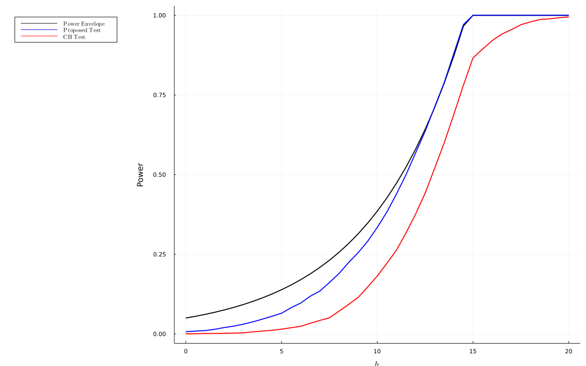
Figure 2. Comparison of NLR test with Wald test based on Chernozhukov and Hong, (2004)

In the supplement (Section B), we present further simulation results for the NLR test with different choices of $\bar{h}$, $\varepsilon$ and sample sizes $n$.

Supplement to “Optimal testing in a class of nonregular models”

Appendix A Mathematical appendix

A.1. Proof of Lemma 1

A.1.1. Proof of (i)

We first consider the case of $\alpha\leq e^{-\bar{h}/\lambda}$. From (4) with $h=0$, we have

$$Z_{n}(0,\bar{h})\rightsquigarrow Z(0,\bar{h})=e^{\bar{h}/\lambda}D_{0,\bar{h}}\quad\text{under }P_{\theta_{0}}.$$ (A.1)

Therefore, it holds

$$\underset{n\to\infty}{\lim\sup}E_{\theta_{0}}[\phi_{n}(Y^{n}|\bar{h},\varepsilon)]$$

$$= \underset{n\to\infty}{\lim}P_{\theta_{0}}\{Z_{n}(0,\bar{h})>e^{\bar{h}/\lambda}(1+\varepsilon)\}+\alpha e^{\bar{h}/\lambda}\underset{n\to\infty}{\lim\sup}P_{\theta_{0}}\{Z_{n}(0,\bar{h})\in[e^{\bar{h}/\lambda}(1-\varepsilon),e^{\bar{h}/\lambda}(1+\varepsilon)]\}$$

$$\leq \Pr\{Z(0,\bar{h})>e^{\bar{h}/\lambda}(1+\varepsilon)\}+\alpha e^{\bar{h}/\lambda}\Pr\{Z(0,\bar{h})\in[e^{\bar{h}/\lambda}(1-\varepsilon),e^{\bar{h}/\lambda}(1+\varepsilon)]\}$$

$$= \Pr\{D_{0,\bar{h}}>1+\varepsilon\}+\alpha e^{\bar{h}/\lambda}\Pr\{D_{0,\bar{h}}=1\}$$

$$= \alpha,$$

where the first equality follows from the definition of $\phi_{n}(Y^{n}|\bar{h},\varepsilon)$ and $P_{\theta_{0}}\{Y_{(1)}<g(\theta_{0})\}=0$, the inequality follows from (A.1), the fact that $Z(0,\bar{h})$ is continuous at $e^{\bar{h}/\lambda}(1+\varepsilon)$ (for the first term), and Portmanteau theorem (for the second term), the second equality follows from the definition of $Z(0,\bar{h})$ and the fact that $D_{0,\bar{h}}$ is binary, and the last equality follows from $\Pr\{D_{0,\bar{h}}>1+\varepsilon\}=0$ and $\Pr\{D_{0,\bar{h}}=1\}=\Pr\{W_{0}>\bar{h}\}=e^{-\bar{h}/\lambda}$.

Similarly, for the case of $\alpha>e^{-\bar{h}/\lambda}$, we have

$$\underset{n\to\infty}{\lim\sup}E_{\theta_{0}}[\phi_{n}(Y^{n}|\bar{h},\varepsilon)]$$

$$= \underset{n\to\infty}{\lim}P_{\theta_{0}}\{Z_{n}(0,\bar{h})>e^{\bar{h}/\lambda}\varepsilon\}+\frac{\alpha-e^{-\bar{h}/\lambda}}{1-e^{-\bar{h}/\lambda}}\underset{n\to\infty}{\lim\sup}P_{\theta_{0}}\{Z_{n}(0,\bar{h})\in[-e^{\bar{h}/\lambda}\varepsilon,e^{\bar{h}/\lambda}\varepsilon]\}$$

$$\leq \Pr\{Z(0,\bar{h})>e^{\bar{h}/\lambda}\varepsilon\}+\frac{\alpha-e^{-\bar{h}/\lambda}}{1-e^{-\bar{h}/\lambda}}\Pr\{Z(0,\bar{h})\in[-e^{\bar{h}/\lambda}\varepsilon,e^{\bar{h}/\lambda}\varepsilon]\}$$

$$= \Pr\{D_{0,\bar{h}}=1\}+\frac{\alpha-e^{-\bar{h}/\lambda}}{1-e^{-\bar{h}/\lambda}}\Pr\{D_{0,\bar{h}}=0\}$$

$$= \alpha,$$

where the first equality follows from the definition of $\phi_{n}(Y^{n}|\bar{h},\varepsilon)$ and $P_{\theta_{0}}\{Y_{(1)}<g(\theta_{0})\}=0$, the inequality follows from (A.1), the fact that $Z(0,\bar{h})$ is continuous at $e^{\bar{h}/\lambda}\varepsilon$ (for the first term), and Portmanteau theorem (for the second term), the second equality follows from the definition of $Z(0,\bar{h})$ and the fact that $D_{0,\bar{h}}$ is binary and $0<e^{\bar{h}/\lambda}\varepsilon<1$, and the last equality follows from $\Pr\{D_{0,\bar{h}}=1\}=e^{-\bar{h}/\lambda}$ and $\Pr\{D_{0,\bar{h}}=0\}=1-e^{-\bar{h}/\lambda}$.

A.1.2. Proof of (ii)

For the case of $\alpha\leq e^{-\bar{h}/\lambda}$, observe that

$$\underset{n\to\infty}{\lim\inf}E_{\theta_{0}+h/n}[\phi_{n}(Y^{n}|\bar{h},\varepsilon)]$$

$$\geq \underset{n\to\infty}{\lim\inf}P_{\theta_{0}+\frac{h}{n}}\{Z_{n}(0,\bar{h})>e^{\bar{h}/\lambda}(1+\varepsilon)\}+\alpha e^{\bar{h}/\lambda}\underset{n\to\infty}{\lim\inf}P_{\theta_{0}+\frac{h}{n}}\{Z_{n}(0,\bar{h})\in[e^{\bar{h}/\lambda}(1-\varepsilon),e^{\bar{h}/\lambda}(1+\varepsilon)]\}$$

$$\geq \alpha e^{\bar{h}/\lambda}\underset{n\to\infty}{\lim\inf}P_{\theta_{0}+\frac{h}{n}}\left\{Z_{n}(h,\bar{h})\in(e^{\bar{h}/\lambda}(1-\varepsilon)Z_{n}(h,0),e^{\bar{h}/\lambda}(1+\varepsilon)Z_{n}(h,0))\right\}$$

$$\geq \alpha e^{\bar{h}/\lambda}\Pr\left\{Z(h,\bar{h})\in(e^{\bar{h}/\lambda}(1-\varepsilon)Z(h,0),e^{\bar{h}/\lambda}(1+\varepsilon)Z(h,0))\right\}$$

$$= \alpha e^{\bar{h}/\lambda}\Pr\left\{\mathbb{I}\{W_{h}>0\}(1-\varepsilon)<\mathbb{I}\{W_{h}>\bar{h}\}<\mathbb{I}\{W_{h}>0\}(1+\varepsilon)\right\}$$

$$= \alpha e^{\bar{h}/\lambda}\Pr\{W_{h}>0,W_{h}>\bar{h}\}$$

$$= \alpha e^{\bar{h}/\lambda}\Pr\{W_{h}>\bar{h}\}$$

$$= \alpha e^{\min\{h,\bar{h}\}/\lambda},$$

where the first inequality follows from the definition of $\phi_{n}(Y^{n}|\bar{h},\varepsilon)$, the second inequality follows from $P_{\theta_{0}+\frac{h}{n}}\{Z_{n}(0,\bar{h})>e^{\bar{h}/\lambda}(1+\varepsilon)\}\geq 0$, $Z_{n}(0,\bar{h})=\frac{Z_{n}(h,\bar{h})}{Z_{n}(h,0)}$, and a set inclusion relationship, the third inequality follows from (4) and Portmanteau theorem, the first equality follows from the definition of $Z(h,\bar{h})$, the second and third equalities follow from set relations, and the last equality follows from the definition of $W_{h}$ and a direct calculation (i.e., $\Pr\{W_{h}>\bar{h}\}=\frac{1}{\lambda}\int_{\max\{\bar{h},h\}}^{\infty}e^{-(w-h)/\lambda}\mathrm{d}w=\min\{e^{(h-\bar{h})/\lambda},1\}$.

Similarly, for the case of $\alpha>e^{-\bar{h}/\lambda}$, we have

$$\underset{n\to\infty}{\lim\inf}E_{\theta_{0}+h/n}[\phi_{n}(Y^{n}|\bar{h},\varepsilon)]$$

$$\geq \underset{n\to\infty}{\lim\inf}P_{\theta_{0}+\frac{h}{n}}\{Z_{n}(0,\bar{h})>e^{\bar{h}/\lambda}\varepsilon\}+\frac{\alpha-e^{-\bar{h}/\lambda}}{1-e^{-\bar{h}/\lambda}}\underset{n\to\infty}{\lim\inf}P_{\theta_{0}+\frac{h}{n}}\{Z_{n}(0,\bar{h})\in[-e^{\bar{h}/\lambda}\varepsilon,e^{\bar{h}/\lambda}\varepsilon]\}$$

$$\geq \underset{n\to\infty}{\lim\inf}P_{\theta_{0}+\frac{h}{n}}\left\{Z_{n}(h,\bar{h})>e^{\bar{h}/\lambda}\varepsilon Z_{n}(h,0)\right\}$$

$$+\frac{\alpha-e^{-\bar{h}/\lambda}}{1-e^{-\bar{h}/\lambda}}\underset{n\to\infty}{\lim\inf}P_{\theta_{0}+\frac{h}{n}}\left\{Z_{n}(h,\bar{h})\in(-e^{\bar{h}/\lambda}\varepsilon Z_{n}(h,0),e^{\bar{h}/\lambda}\varepsilon Z_{n}(h,0))\right\}$$

$$\geq \Pr\left\{Z(h,\bar{h})>e^{\bar{h}/\lambda}\varepsilon Z(h,0)\right\}+\frac{\alpha-e^{-\bar{h}/\lambda}}{1-e^{-\bar{h}/\lambda}}\Pr\left\{Z(h,\bar{h})\in(-e^{\bar{h}/\lambda}\varepsilon Z(h,0),e^{\bar{h}/\lambda}\varepsilon Z(h,0))\right\}$$

$$= \Pr\{\mathbb{I}\{W_{h}>\bar{h}\}>\mathbb{I}\{W_{h}>0\}\varepsilon\}+\frac{\alpha-e^{-\bar{h}/\lambda}}{1-e^{-\bar{h}/\lambda}}\Pr\left\{-\mathbb{I}\{W_{h}>0\}\varepsilon<\mathbb{I}\{W_{h}>\bar{h}\}<\mathbb{I}\{W_{h}>0\}\varepsilon\right\}$$

$$= \Pr\{W_{h}>\bar{h}\}+\frac{\alpha-e^{-\bar{h}/\lambda}}{1-e^{-\bar{h}/\lambda}}(1-\Pr\{W_{h}>\bar{h}\})$$

$$= \frac{\alpha-e^{-\bar{h}/\lambda}}{1-e^{-\bar{h}/\lambda}}+\min\{e^{(h-\bar{h})/\lambda},1\}\frac{1-\alpha}{1-e^{-\bar{h}/\lambda}},$$

where the first inequality follows from the definition of $\phi_{n}(Y^{n}|\bar{h},\varepsilon)$, the second inequality follows from $Z_{n}(0,\bar{h})=\frac{Z_{n}(h,\bar{h})}{Z_{n}(h,0)}$ and a set inclusion relation, the third inequality follows from (4) the fact that $Z(h,\bar{h})/Z(h,0)$ is continuous at $e^{\bar{h}/\lambda}\varepsilon$ (for the first term), and Portmanteau theorem (for the second term), the first equality follows from the definition of $Z(h,\bar{h})$, the second equality follows from set relations, and the last equality follows from the definition of $W_{h}$.

A.1.3. Proof of (iii)

In this proof, let $P_{h}\{\cdot\}$ and $E_{h}[\cdot]$ be the probability and the expectation under $f_{W}(w|h)$, and define $\alpha(k)=P_{0}\{f_{W}(W|\bar{h})>kf_{W}(W|0)\}$. Pick any $\alpha\in(0,1)$ and let $k_{0}$ be such that $\alpha(k_{0})\leq\alpha\leq\alpha(k_{0}-0)$. Then the Neyman-Pearson test is defined as

$$\phi(W)=\left\{\begin{array}[]{lll}1&\text{if}&f_{W}(W|\bar{h})>k_{0}f_{W}(W|0)\\ \frac{\alpha-\alpha(k_{0})}{\alpha(k_{0}-0)-\alpha(k_{0})}&\text{if}&f_{W}(W|\bar{h})=k_{0}f_{W}(W|0)\\ 0&\text{if}&f_{W}(W|\bar{h})<k_{0}f_{W}(W|0)\end{array}\right..$$

Note that this test satisfies $E_{0}[\phi(W)]=\alpha$. By Neyman-Pearson lemma (e.g., Theorem 3.2.1 (ii) of Lehmann and Romano,, 2022), this test is most powerful. Letting $Z(h,\bar{h})=e^{(\bar{h}-h)/\lambda}\mathbb{I}\{W>\bar{h}\}$, observe that

$$f_{W}(W|\bar{h})\gtreqless k_{0}f_{W}(W|0)\text{ if and only if }Z(\bar{h},\bar{h})\gtreqless k_{0}Z(\bar{h},0).$$

Thus, $\phi(W)$ can be alternatively written as

$$\phi(W) = \left\{\begin{array}[]{lll}1&\text{if}&Z(\bar{h},\bar{h})>k_{0}Z(\bar{h},0)\\ \frac{\alpha-\alpha(k_{0})}{\alpha(k_{0}-0)-\alpha(k_{0})}&\text{if}&Z(\bar{h},\bar{h})=k_{0}Z(\bar{h},0)\\ 0&\text{if}&Z(\bar{h},\bar{h})<k_{0}Z(\bar{h},0)\end{array}\right..$$

By computing $k_{0}$ and $\frac{\alpha-\alpha(k_{0})}{\alpha(k_{0}-0)-\alpha(k_{0})}$ for the each case, $\phi(W)$ becomes

$$\phi(W)=\begin{cases}\left\{\begin{array}[]{lll}1&\text{if}&Z(\bar{h},\bar{h})>e^{\bar{h}/\lambda}Z(\bar{h},0)\\ \alpha e^{\bar{h}/\lambda}&\text{if}&Z(\bar{h},\bar{h})=e^{\bar{h}/\lambda}Z(\bar{h},0)\\ 0&\text{if}&Z(\bar{h},\bar{h})<e^{\bar{h}/\lambda}Z(\bar{h},0)\end{array}\right.&\text{for }\alpha\leq e^{-\bar{h}/\lambda}\\ \left\{\begin{array}[]{lll}1&\text{if}&Z(\bar{h},\bar{h})>0\cdot Z(\bar{h},0)\\ \frac{\alpha-e^{-\bar{h}/\lambda}}{1-e^{-\bar{h}/\lambda}}&\text{if}&Z(\bar{h},\bar{h})=0\cdot Z(\bar{h},0)\\ 0&\text{if}&Z(\bar{h},\bar{h})<0\cdot Z(\bar{h},0)\end{array}\right.&\text{for }\alpha>e^{-\bar{h}/\lambda}\end{cases}.$$

For this test, we now compute the power function $\Pi(\bar{h})=\int\phi(w)\mathrm{d}P_{\bar{h}}(w)$. When $\alpha\leq e^{-\bar{h}/\lambda}$, it holds

$$\Pi(\bar{h}) = \Pr\left\{Z(\bar{h},\bar{h})>e^{\bar{h}/\lambda}Z(\bar{h},0)\right\}+\alpha e^{\bar{h}/\lambda}\Pr\left\{Z(\bar{h},\bar{h})=e^{\bar{h}/\lambda}Z(\bar{h},0)\right\}$$

$$= \Pr\left\{\underbrace{\mathbb{I}\{W_{\bar{h}}>\bar{h}\}}_{=1}>\underbrace{\mathbb{I}\{W_{\bar{h}}>0\}}_{=1}\right\}+\alpha e^{\bar{h}/\lambda}\Pr\{\mathbb{I}\{W_{\bar{h}}>\bar{h}\}=\mathbb{I}\{W_{\bar{h}}>0\}=1\}$$

$$= \alpha e^{\bar{h}/\lambda}.$$

Also when $\alpha>e^{-\bar{h}/\lambda}$, we have

$$\Pi(\bar{h}) = \Pr\left\{Z(\bar{h},\bar{h})>0\right\}+\frac{\alpha-e^{-\bar{h}/\lambda}}{1-e^{-\bar{h}/\lambda}}\Pr\left\{Z(\bar{h},\bar{h})=0\right\}$$

$$= \Pr\{W_{\bar{h}}>\bar{h}\}=1.$$

Finally, the inequality $\Pi(h)\geq\pi_{L}(h,\bar{h})$ for any $h,\bar{h}>0$ is obvious.

A.2. Proof of Theorem 1

Pick any $h\geq 0$ and any sequence of tests $\{\psi_{n}\}$ satisfying $\limsup_{n}E_{\theta_{0}}[\psi_{n}]\leq\alpha$. Lemma 1 (i) guarantees $\limsup_{n}E_{\theta_{0}}[\phi_{n}(Y^{n}|\bar{h}^{+},\varepsilon)]\leq\alpha$. Also Lemma 1 (ii) with $\alpha=e^{-\bar{h}^{+}/\lambda}$ implies

$$\liminf_{n}E_{\theta_{0}+\frac{h}{n}}[\phi_{n}(Y^{n}|\bar{h}^{+},\varepsilon)]\geq\alpha e^{\min\{h,\bar{h}^{+}\}/\lambda}=\begin{cases}\alpha e^{h/\lambda}&\text{ if }\alpha\leq e^{-h/\lambda}\\ 1&\text{ if }\alpha>e^{-h/\lambda}\end{cases}=\Pi(h),$$

where the first equality follows from $\alpha=e^{-\bar{h}^{+}/\lambda}$ . Thus, it is sufficient to show that

$$\Pi(h)\geq\limsup_{n}E_{\theta_{0}+\frac{h}{n}}[\psi_{n}].$$ (A.3)

Consider a subsequence $\{\psi_{m}\}$ of $\{\psi_{n}\}$ such that

$$\lim_{m}E_{\theta_{0}}[\psi_{m}] \leq \limsup_{n}E_{\theta_{0}}[\psi_{n}]\leq\alpha,$$

$$\lim_{m}E_{\theta_{0}+\frac{h}{m}}[\psi_{m}] = \limsup_{n}E_{\theta_{0}+\frac{h}{n}}[\psi_{n}].$$

By Van der Vaart, (2000, Theorem 15.1), if a sequence of power functions of tests $\{E_{\theta_{0}+\frac{h}{m}}[\psi_{m}]\}$ pointwise converges to a some function (denoted by $\pi_{\psi}(h)$) for every $h$, then, this $\pi_{\psi}(h)$ is a power function for testing $H_{0}^{W}:h=0$ against $H_{1}^{W+}:h>0$ in one sample $W\sim f_{W}(w|h)$. On the other hand, Lemma 1 (iii) implies that $\Pi(\bar{h})$ is power of the Neyman-Pearson test for $H_{0}^{W}:h=0$ against $H_{1}^{W}:h=\bar{h}$ in one sample $W\sim f_{W}(w|h)$. Therefore, we have $\Pi(h)\geq\pi_{\psi}(h)$, which implies (A.3) and the conclusion is obtained.

A.3. Proof of Lemma 2

A.3.1. Proof of (i)

By a similar argument to the proof of Lemma 1 (i), we have

$$\underset{n\to\infty}{\lim\sup}E_{\theta_{0}}[\phi_{n}(Y^{n}|\bar{h},\varepsilon)]$$

$$= \underset{n\to\infty}{\lim}P_{\theta_{0}}\{Z_{n}(0,\bar{h})>e^{\bar{h}/\lambda}(1+\varepsilon)\}+\alpha\underset{n\to\infty}{\lim\sup}P_{\theta_{0}}\{Z_{n}(0,\bar{h})\in[e^{\bar{h}/\lambda}(1-\varepsilon),e^{\bar{h}/\lambda}(1+\varepsilon)]\}$$

$$\leq \Pr\{Z(0,\bar{h})>e^{\bar{h}/\lambda}(1+\varepsilon)\}+\alpha\Pr\{Z(0,\bar{h})\in[e^{\bar{h}/\lambda}(1-\varepsilon),e^{\bar{h}/\lambda}(1+\varepsilon)]\}$$

$$= \Pr\{D_{0,\bar{h}}>1+\varepsilon\}+\alpha\Pr\{D_{0,\bar{h}}=1\}$$

$$= \alpha,$$

where the last equality follows from $\Pr\{D_{0,\bar{h}}=1\}=\Pr\{W_{0}>\bar{h}\}=1$ for any $\bar{h}<0$.

A.3.2. Proof of (ii)

By a similar argument to the proof of Lemma 1 (ii), we have

$$\underset{n\to\infty}{\lim\inf}E_{\theta_{0}+h/n}[\phi_{n}(Y^{n}|\bar{h},\varepsilon)]$$

$$\geq \underset{n\to\infty}{\lim\inf}P_{\theta_{0}+\frac{h}{n}}\left\{Z_{n}(h,\bar{h})>e^{\bar{h}/\lambda}(1+\varepsilon)Z_{n}(h,0)\right\}$$

$$+\alpha\underset{n\to\infty}{\lim\inf}P_{\theta_{0}+\frac{h}{n}}\left\{Z_{n}(h,\bar{h})\in(e^{\bar{h}/\lambda}(1-\varepsilon)Z_{n}(h,0),e^{\bar{h}/\lambda}(1+\varepsilon)Z_{n}(h,0))\right\}$$

$$\geq \Pr\left\{Z(h,\bar{h})>e^{\bar{h}/\lambda}(1+\varepsilon)Z(h,0)\right\}+\alpha\Pr\left\{Z(h,\bar{h})\in(e^{\bar{h}/\lambda}(1-\varepsilon)Z(h,0),e^{\bar{h}/\lambda}(1+\varepsilon)Z(h,0))\right\}$$

$$= \Pr\{\mathbb{I}\{W_{h}>\bar{h}\}>\mathbb{I}\{W_{h}>0\}(1+\varepsilon)\}+\alpha\Pr\{\mathbb{I}\{W_{h}>0\}(1-\varepsilon)<\mathbb{I}\{W_{h}>\bar{h}\}<\mathbb{I}\{W_{h}>0\}(1+\varepsilon)\}$$

$$= \Pr\{\bar{h}<W_{h}\leq 0\}+\alpha\Pr\{W_{h}>0,W_{h}>\bar{h}\}$$

$$= \Pr\{\bar{h}<W_{h}\leq 0\}+\alpha\Pr\{W_{h}>0\}$$

$$= \min\{e^{(h-\bar{h})/\lambda},1\}-(1-\alpha)e^{h/\lambda},$$

where the first inequality follows from the definition of $\phi_{n}(Y^{n}|\bar{h},\varepsilon)$ and set inclusion relations, the second inequality follows from (4), the fact that $Z(h,\bar{h})/Z(h,0)$ is continuous at $e^{\bar{h}/\lambda}(1+\varepsilon)$ (for the first term), and Portmanteau theorem (for the second term), the first equality follows from the definition of $Z(h,\bar{h})$, the second and third equalities follow from set relations, and the last equality follows from direct calculations, i.e.,

$$\Pr\{\bar{h}<W_{h}\leq 0\} = \frac{1}{\lambda}\int_{\max\{\bar{h},h\}}^{0}e^{-(w-h)/\lambda}\mathrm{d}w=\min\{e^{(h-\bar{h})/\lambda},1\}-e^{h/\lambda},$$

$$\Pr\{W_{h}>0\} = \frac{1}{\lambda}\int_{0}^{\infty}e^{-(w-h)/\lambda}\mathrm{d}w=e^{h/\lambda}.$$

A.3.3. Proof of (iii)

Similarly to the proof of Lemma 1 (iii), Neyman-Pearson lemma implies that

$$\phi(W) = \left\{\begin{array}[]{lll}1&\text{if}&Z(\bar{h},\bar{h})>e^{\bar{h}/\lambda}Z(\bar{h},0)\\ \alpha&\text{if}&Z(\bar{h},\bar{h})=e^{\bar{h}/\lambda}Z(\bar{h},0)\\ 0&\text{if}&Z(\bar{h},\bar{h})<e^{\bar{h}/\lambda}Z(\bar{h},0)\end{array}\right.,$$

is the most powerful test. For this test, its power is obtained as

$$\Pi(\bar{h}) = \Pr\left\{Z(\bar{h},\bar{h})>e^{\bar{h}/\lambda}Z(\bar{h},0)\right\}+\alpha\Pr\left\{Z(\bar{h},\bar{h})=e^{\bar{h}/\lambda}Z(\bar{h},0)\right\}$$

$$= \Pr\left\{\underbrace{\mathbb{I}\{W_{\bar{h}}>\bar{h}\}}_{=1}>\mathbb{I}\{W_{\bar{h}}>0\}\right\}+\alpha\Pr\{\mathbb{I}\{W_{\bar{h}}>\bar{h}\}=\mathbb{I}\{W_{\bar{h}}>0\}=1\}$$

$$= \Pr\{W_{\bar{h}}\leq 0\}+\alpha\Pr\{W_{\bar{h}}>0\}$$

$$= 1-(1-\alpha)\Pr\{W_{\bar{h}}>0\}$$

$$= 1-(1-\alpha)e^{\bar{h}/\lambda}.$$

Finally, the inequality $\Pi(h)\geq\pi_{L}(h,\bar{h})$ for any $h,\bar{h}<0$ is obvious.

A.4. Proof of Theorem 2

Pick any $h\leq 0$ and any sequence of tests $\{\psi_{n}\}$ satisfying $\limsup_{n}E_{\theta_{0}}[\psi_{n}]\leq\alpha$. Lemma 2 (i) guarantees $\limsup_{n}E_{\theta_{0}}[\phi_{n}(Y^{n}|\bar{h}^{-},\varepsilon)]\leq\alpha$. Also Lemma 2 (ii) implies

$$\liminf_{n}E_{\theta_{0}+\frac{h}{n}}[\phi_{n}(Y^{n}|\bar{h}^{-},\varepsilon)] \geq \min\{e^{(h-\bar{h}^{-})/\lambda},1\}-(1-\alpha)e^{h/\lambda}=1-(1-\alpha)e^{h/\lambda}=\Pi(h)$$

$$\geq \limsup_{n}E_{\theta_{0}+\frac{h}{n}}[\psi_{n}].$$

where the first equality follows from $\bar{h}^{-}<h$ for any $h\leq 0$ in $\mathcal{H}$, and the second inequality follows from the same argument to obtain (A.3) by Lemma 2 (iii).

A.5. Proof of Theorem 3

The proof has three steps. First, we will show that the asymptotic size is $\alpha$, $\underset{n\to\infty}{\lim\sup}E_{\theta_{0}}[\phi_{n}(Y^{n}|\bar{h}^{+},\bar{h}^{-},\varepsilon)]\leq\alpha$. Next, we will derive the lower bound for $\underset{n\to\infty}{\lim\inf}E_{\theta_{0}+h/n}[\phi_{n}(Y^{n}|\bar{h}^{+},\bar{h}^{-},\varepsilon)]$. Finally, we will prove that $\phi_{n}(Y^{n}|\bar{h}^{+},\bar{h}^{-},\varepsilon)$ satisfies the definition of AUMP.

A.5.1. Size control.

By a similar argument to the proof of Lemma 1 (i), we have

$$\underset{n\to\infty}{\lim\sup}E_{\theta_{0}}[\phi_{n}(Y^{n}|\bar{h}^{+},\bar{h}^{-},\varepsilon)]$$

$$\leq \underset{n\to\infty}{\lim}P_{\theta_{0}}\left\{Z_{n}(0,\bar{h}^{+})\geq e^{\bar{h}^{+}/\lambda}(1-\varepsilon)\right\}+\underset{n\to\infty}{\lim}P_{\theta_{0}}\left\{Z_{n}(0,\bar{h}^{-})>e^{\bar{h}^{-}/\lambda}(1+\varepsilon)\right\}$$

$$= \Pr\left\{Z(0,\bar{h}^{+})\geq e^{\bar{h}^{+}/\lambda}(1-\varepsilon)\right\}+\Pr\left\{Z(0,\bar{h}^{-})>e^{\bar{h}^{-}/\lambda}(1+\varepsilon)\right\}$$

$$= \Pr\left\{D_{0,\bar{h}^{+}}\geq(1-\varepsilon)\right\}+\Pr\left\{D_{0,\bar{h}^{-}}>(1+\varepsilon)\right\}$$

$$= \Pr\left\{D_{0,\bar{h}^{+}}=1\right\}$$

$$= \min\left\{e^{-\bar{h}^{+}/\lambda},1\right\}$$

$$= \alpha,$$

where the inequality follows from the definition of $\phi_{n}(Y^{n}|\bar{h}^{+},\bar{h}^{-},\varepsilon)$, the union bound, and $P_{\theta_{0}}\{Y_{(1)}<g(\theta_{0})\}=0$, the first equality follows from (A.1), the fact that $Z(0,\bar{h}^{+})$ is continuous at $e^{\bar{h}^{+}/\lambda}(1-\varepsilon)$ (for the first term) and the fact that $Z(0,\bar{h}^{-})$ is continuous at $e^{\bar{h}^{-}/\lambda}(1+\varepsilon)$ (for the second term), the second equality follows from the definition of $Z(0,\bar{h})$, the third equality follows by the fact that $D_{0,\bar{h}}$ is binary, the fourth equality follows from $\Pr\{D_{0,\bar{h}^{+}}=1\}=\Pr\{W_{0}>\bar{h}^{+}\}=e^{-\bar{h}^{+}/\lambda}$, and the last equality follows by the construction of $\bar{h}^{+}$.

A.5.2. Lower bound of power.

By a similar argument to the proof of Lemma 1 (ii), we have

$$\underset{n\to\infty}{\lim\inf}E_{\theta_{0}+h/n}[\phi_{n}(Y^{n}|\bar{h}^{+},\bar{h}^{-},\varepsilon)]$$

$$\geq \underset{n\to\infty}{\lim\inf}P_{\theta_{0}+\frac{h}{n}}\left\{Z_{n}(0,\bar{h}^{+})\geq e^{\bar{h}^{+}/\lambda}(1-\varepsilon)\text{ or }Z_{n}(0,\bar{h}^{-})>e^{\bar{h}^{-}/\lambda}(1+\varepsilon)\right\}$$

$$\geq \underset{n\to\infty}{\lim\inf}P_{\theta_{0}+\frac{h}{n}}\left\{Z_{n}\left(0,\bar{h}^{+}\right)\in\left(e^{\bar{h}^{+}/\lambda}(1-\varepsilon),e^{\bar{h}^{+}/\lambda}(1+\varepsilon)\right)\text{ or }Z_{n}\left(0,\bar{h}^{-}\right)>e^{\bar{h}^{-}/\lambda}(1+\varepsilon)\right\}$$

$$\geq \underset{n\to\infty}{\lim\inf}P_{\theta_{0}+\frac{h}{n}}\left\{Z_{n}\left(h,\bar{h}^{+}\right)\in\left(e^{\bar{h}^{+}/\lambda}(1-\varepsilon)Z_{n}(h,0),e^{\bar{h}^{+}/\lambda}(1+\varepsilon)Z_{n}(h,0)\right)\right.$$

$$\qquad\qquad\qquad\qquad\left.\text{ or }Z_{n}\left(h,\bar{h}^{-}\right)>e^{\bar{h}^{-}/\lambda}(1+\varepsilon)Z_{n}(h,0)\right\}$$

$$\geq \Pr\left\{Z\left(h,\bar{h}^{+}\right)\in\left(e^{\bar{h}^{+}/\lambda}(1-\varepsilon)Z(h,0),e^{\bar{h}^{+}/\lambda}(1+\varepsilon)Z(h,0)\right)\text{ or }Z\left(h,\bar{h}^{-}\right)>e^{\bar{h}^{-}/\lambda}(1+\varepsilon)Z(h,0)\right\}$$

$$= \Pr\left\{D_{h,\bar{h}^{+}}\in\left((1-\varepsilon)D_{h,0},(1+\varepsilon)D_{h,0}\right)\text{ or }D_{h,\bar{h}^{-}}>(1+\varepsilon)D_{h,0}\right\}$$

$$= \Pr\left\{\mathbb{I}\left\{W_{h}>\bar{h}^{+}\right\}\in\left((1-\varepsilon)\mathbb{I}\{W_{h}>0\},(1+\varepsilon)\mathbb{I}\{W_{h}>0\}\right)\text{ or }\mathbb{I}\left\{W_{h}>\bar{h}^{-}\right\}\geq\mathbb{I}\{W_{h}>0\}(1+\varepsilon)\right\}$$

$$= \Pr\left\{\left(W_{h}>0\text{ and }W_{h}>\bar{h}^{+}\right)\text{ or }\bar{h}^{-}<W_{h}\leq 0\right\}$$

$$= \Pr\left\{W_{h}>\bar{h}^{+}\text{ or }W_{h}\leq 0\right\}$$

$$= \Pr\left\{W_{h}>\bar{h}^{+}\right\}+\Pr\left\{W_{h}\leq 0\right\}$$

$$= \min\left\{e^{\left(h-\bar{h}^{+}\right)/\lambda},1\right\}+1-\min\left\{e^{h/\lambda},1\right\}$$

$$= \min\left\{\alpha e^{h/\lambda},1\right\}+1-\min\left\{e^{h/\lambda},1\right\},$$

where the first inequality follows from the definition of $\phi_{n}(Y^{n}|\bar{h}^{+},\bar{h}^{-},\varepsilon)$, the second inequality follows from a set inclusion relationship, the third inequality follows from $Z_{n}(0,\bar{h})=\frac{Z_{n}(h,\bar{h})}{Z_{n}(h,0)}$, the fourth inequality follows from (4) and Portmanteau theorem, the first equality follows from the definition of $Z(h,\bar{h})$, the second equality follows from the definition of $D_{h,\bar{h}}$, the third and forth equalities follow from set relations, $\bar{h}^{+}>0$, and $\bar{h}^{-}=-M$, the fifth equality follows from $\left\{W_{h}>\bar{h}^{+}\text{ and }W_{h}\leq 0\right\}=\emptyset$, the sixth equalities follows from $\Pr\{W_{h}>\bar{h}\}=\min\{e^{(h-\bar{h})/\lambda},1\}$, and the last equality follows by the construction of $\bar{h}^{+}$.

A.5.3. Optimality.

The lower bound equals to the power envelope:

$$\underset{n\to\infty}{\lim\inf}E_{\theta_{0}+h/n}[\phi_{n}(Y^{n}|\bar{h}^{+},\bar{h}^{-},\varepsilon)] \geq\min\left\{\alpha e^{h/\lambda},1\right\}+1-\min\left\{e^{h/\lambda},1\right\}$$

$$=\begin{cases}\alpha e^{h/\lambda}&\text{ if }\alpha\leq e^{-h/\lambda}\text{ and }h>0\\ 1&\text{ if }\alpha>e^{-h/\lambda}\text{ and }h>0\\ 1-(1-\alpha)e^{h/\lambda}&\text{ if }h<0\end{cases}$$

$$=\Pi\left(h\right),$$

where $\Pi\left(h\right)$ is derived in proofs of Lemma 1 (iii) and Lemma 2 (iii). Pick any $h\in\mathcal{H}$ and any sequence of tests $\{\psi_{n}\}$ satisfying $\limsup_{n}E_{\theta_{0}}[\psi_{n}]\leq\alpha$. Lemma 1 (iii) and Lemma 2 (iii) imply that $\Pi(\bar{h})$ is power of the Neyman-Pearson test for $H_{0}^{W}:h=0$ against $H_{1}^{W}:h=\bar{h}$ in one sample $W\sim f_{W}(w|h)$ for any $\bar{h}\in\mathcal{H}$. Thus, we have

$$\Pi(h)\geq\limsup_{n}E_{\theta_{0}+\frac{h}{n}}[\psi_{n}]$$ (A.5)

by the same argument to obtain (A.3).

A.6. Proof of Lemma 3

Let $\delta_{n}=n^{-1/4}$. Pick any $h$, $\bar{h}\in I$, and $z$. Observe that

$$\underset{n\to\infty}{\lim}P_{\theta_{0}+\frac{h}{n},\gamma}\{Z(h,\check{h}_{n},\check{\gamma}_{n})\leq z\}$$

$$= \underset{n\to\infty}{\lim}P_{\theta_{0}+\frac{h}{n},\gamma}\{Z(h,\check{h}_{n},\check{\gamma}_{n})\leq z,|\check{h}_{n}-\bar{h}|+\left\|\check{\gamma}_{n}-\gamma\right\|\leq\delta_{n}\}$$

$$+\underset{n\to\infty}{\lim}P_{\theta_{0}+\frac{h}{n},\gamma}\{Z(h,\check{h}_{n},\check{\gamma}_{n})\leq z,|\check{h}_{n}-\bar{h}|+\left\|\check{\gamma}_{n}-\gamma\right\|>\delta_{n}\}$$

$$= \underset{n\to\infty}{\lim}P_{\theta_{0}+\frac{h}{n},\gamma}\{Z(h,\check{h}_{n},\check{\gamma}_{n})\leq z,|\check{h}_{n}-\bar{h}|+\left\|\check{\gamma}_{n}-\gamma\right\|\leq\delta_{n}\}$$

$$= \underset{n\to\infty}{\lim}P_{\theta_{0}+\frac{h}{n},\gamma}\{Z(h,\check{h}_{n},\check{\gamma}_{n})\leq z\text{ }|\text{ }|\check{h}_{n}-\bar{h}|+\left\|\check{\gamma}_{n}-\gamma\right\|\leq\delta_{n}\}P_{\theta_{0}+\frac{h}{n},\gamma}\{|\check{h}_{n}-\bar{h}|+\left\|\check{\gamma}_{n}-\gamma\right\|\leq\delta_{n}\},$$

where the first equality follows from the set relationship, and the second equality follows from

$$P_{\theta_{0}+\frac{h}{n},\gamma}\{Z(h,\check{h}_{n},\check{\gamma}_{n})\leq z,|\check{h}_{n}-\bar{h}|+\left\|\check{\gamma}_{n}-\gamma\right\|>\delta_{n}\}\leq P_{\theta_{0}+\frac{h}{n},\gamma}\{|\check{h}_{n}-\bar{h}|+\left\|\check{\gamma}_{n}-\gamma\right\|>\delta_{n}\}\rightarrow 0.$$

Thus, under $P_{\theta_{0}+\frac{h}{n},\gamma}$ conditional on $|\check{h}_{n}-\bar{h}|+\left\|\check{\gamma}_{n}-\gamma\right\|\leq\delta_{n}$,

$$Z_{n}(h,\check{h}_{n},\check{\gamma}_{n})$$

$$= \prod_{i=1}^{n}\frac{f(Y_{i}|X_{i},\theta_{0}+\check{h}_{n}/n,\check{\gamma}_{n})\mathbb{I}\{Y_{i}\geq g(X_{i},\theta_{0}+\check{h}_{n}/n)\}}{f(Y_{i}|X_{i},\theta_{0}+h/n,\check{\gamma}_{n})\mathbb{I}\{Y_{i}\geq g(X_{i},\theta_{0}+h/n)\}}$$

$$\geq \prod_{i=1}^{n}\frac{f(Y_{i}|X_{i},\theta_{0}+\check{h}_{n}/n,\check{\gamma}_{n})\mathbb{I}\{Y_{i}\geq g(X_{i},\theta_{0}+\bar{h}/n+n^{-3/2})\}}{f(Y_{i}|X_{i},\theta_{0}+h/n,\check{\gamma}_{n})\mathbb{I}\{Y_{i}\geq g(X_{i},\theta_{0}+h/n)\}},$$

where the equality follows by the definition of $Z_{n}$, and the inequality holds eventually by the continuity assumption of $\nabla_{\theta}g(X_{i},\theta_{0})>0$. Now define

$$D_{n} = \prod_{i=1}^{n}\mathbb{I}\{Y_{i}\geq g(X_{i},\theta_{0}+\bar{h}/n+n^{-3/2})\},$$

$$R_{n} = \sum_{i=1}^{n}\{\log f(Y_{i}|X_{i},\theta_{0}+\check{h}_{n}/n,\check{\gamma}_{n})-\log f(Y_{i}|X_{i},\theta_{0}+h/n,\check{\gamma}_{n})\}.$$

First, we show that $D_{n}\rightsquigarrow D_{h,\bar{h}}$ under $P_{\theta_{0}+\frac{h}{n},\gamma}$. Let $\bar{\theta}_{n}=\theta_{0}+\bar{h}/n+n^{-3/2}$. Under $P_{\theta_{0}+\frac{h}{n},\gamma}$, we have

$$D_{n}=\prod_{i=1}^{n}\mathbb{I}\{Y_{i}\geq g(X_{i},\bar{\theta}_{n})\}\rightsquigarrow\mathrm{Bernoulli}\left(\lim_{n\rightarrow\infty}E_{\theta_{0}+\frac{h}{n},\gamma}\left[\prod_{i=1}^{n}\mathbb{I}\{Y_{i}\geq g(X_{i},\bar{\theta}_{n})\}\right]\right).$$

Let’s compute $\lim_{n\rightarrow\infty}E_{\theta_{0}+\frac{h}{n},\gamma}\left[\prod_{i=1}^{n}\mathbb{I}\{Y_{i}\geq g(X_{i},\bar{\theta}_{n})\}\right]$. Note that for some $\grave{h}_{n}$ such that $g(x,\theta_{0}+\grave{h}_{n}/n)$ is between $g(x,\theta_{0}+\bar{h}/n+n^{-3/2})$ and $g(x,\theta_{0}+h/n)$, and some $\tilde{\theta}_{n}$ is between $\theta_{0}+\bar{h}/n+n^{-3/2}$ and $\theta_{0}+h/n$, it holds

$$E_{\theta_{0}+\frac{h}{n},\gamma}[\mathbb{I}\{Y\geq g(X,\bar{\theta}_{n})\}]$$

$$= 1-E_{X}[F_{Y\mid X,\theta_{0}+\frac{h}{n},\gamma}(g(X,\bar{\theta}_{n}))]$$

$$= 1-E_{X}\left[\int_{-\infty}^{g(X,\bar{\theta}_{n})}f(y|X,\theta_{0}+h/n,\gamma)\mathbb{I}\{y-g(X,\theta_{0}+h/n)\geq 0\}dy\right]$$

$$= 1-E_{X}\left[\mathbb{I}\{g(X,\bar{\theta}_{n})-g(X,\theta_{0}+h/n)\geq 0\}\int_{g(X,\theta_{0}+h/n)}^{g(X,\bar{\theta}_{n})}f(y|X,\theta_{0}+h/n,\gamma)dy\right]$$

$$= 1-E_{X}\left[\begin{array}[]{c}\mathbb{I}\{g(X,\bar{\theta}_{n})-g(X,\theta_{0}+h/n)\geq 0\}\\ \times f(g(X,\theta_{0}+\grave{h}_{n}/n)|X,\theta_{0}+h/n,\gamma)\{g(X,\bar{\theta}_{n})-g(X,\theta_{0}+h/n)\}\end{array}\right]$$

$$= 1-E_{X}\left[\begin{array}[]{c}\mathbb{I}\{\nabla_{\theta}g(X,\tilde{\theta}_{n})(\bar{h}+n^{-1/2}-h)\geq 0\}\\ \times f(g(X,\theta_{0}+\grave{h}_{n}/n)|X,\theta_{0}+h/n,\gamma)\nabla_{\theta}g(X,\tilde{\theta}_{n})(\bar{h}+n^{-1/2}-h)/n\end{array}\right]$$

where where the second inequality follows from the model (12), the fourth equality follows from an expansion of $\int_{g(X,\theta_{0}+h/n)}^{g(X,\bar{\theta}_{n})}f(y|X,\theta_{0}+h/n,\gamma)dy$ around $g(x,\bar{\theta}_{n})=g(X,\theta_{0}+h/n)$, and the fifth equality follows from an expansion of $g(x,\bar{\theta}_{n})$ around $\bar{\theta}_{n}=\theta_{0}+h/n$. Thus, recalling that $\bar{\theta}_{n}$ and $\tilde{\theta}_{n}$ are non-random, we have

$$E_{\theta_{0}+\frac{h}{n},\gamma}\left[\prod_{i=1}^{n}\mathbb{I}\{Y_{i}\geq g(X_{i},\bar{\theta}_{n})\}\right]=[P_{\theta_{0}+\frac{h}{n},\gamma}\{Y\geq g(X,\bar{\theta}_{n})\}]^{n}$$

$$= \left[1-\frac{1}{n}E_{X}\left[\begin{array}[]{c}\mathbb{I}\{\nabla_{\theta}g(X,\tilde{\theta}_{n})(\bar{h}+n^{-1/2}-h)\geq 0\}\\ \times f(g(X,\theta_{0}+\grave{h}_{n}/n)|X,\theta_{0}+h/n,\gamma)\nabla_{\theta}g(X,\tilde{\theta}_{n})(\bar{h}+n^{-1/2}-h)\end{array}\right]\right]^{n}$$

$$\rightarrow \exp\left(\lim_{n\rightarrow\infty}-E_{X}\left[\begin{array}[]{c}\mathbb{I}\{\nabla_{\theta}g(X,\tilde{\theta}_{n})(\bar{h}+n^{-1/2}-h)\geq 0\}\\ \times f(g(X,\theta_{0}+\grave{h}_{n}/n)|X,\theta_{0}+h/n,\gamma)\nabla_{\theta}g(X,\tilde{\theta}_{n})(\bar{h}+n^{-1/2}-h)\end{array}\right]\right)$$

$$= \exp\left(-E_{X}\left[\lim_{n\rightarrow\infty}\left[\begin{array}[]{c}\mathbb{I}\{\nabla_{\theta}g(X,\tilde{\theta}_{n})(\bar{h}+n^{-1/2}-h)\geq 0\}\\ \times f(g(X,\theta_{0}+\grave{h}_{n}/n)|X,\theta_{0}+h/n,\gamma)\nabla_{\theta}g(X,\tilde{\theta}_{n})(\bar{h}+n^{-1/2}-h)\end{array}\right]\right]\right)$$

$$= \exp\left(-E_{X}\left[\begin{array}[]{c}\lim_{n\rightarrow\infty}\mathbb{I}\{\nabla_{\theta}g(X,\tilde{\theta}_{n})(\bar{h}+n^{-1/2}-h)\geq 0\}\\ \times f(g(X,\theta_{0})|X,\theta_{0},\gamma)\nabla_{\theta}g(X,\theta_{0})(\bar{h}-h)\end{array}\right]\right),$$

where the first equality follows from the iid assumption, the second equality follows from the calculation above, the third equality follows from the dominated convergence theorem with the uniform boundedness of $f(y|x,\theta,\gamma)$ and $\sup_{\beta\in\mathcal{N}}\left\|\nabla_{\theta}g(x,\theta)\right\|<\infty$, and the last equality follows from the continuity of $f(y|x,\theta,\gamma)$ in $y$ and $\theta$ and the continuity of $g(x,\theta)$ and $\nabla_{\theta}g(x,\theta)$ in $\theta$. Since the assumption $\nabla_{\theta}g(a_{j},\theta_{0})>0$ guarantees

$$\lim_{n\rightarrow\infty}\mathbb{I}\{\nabla_{\theta}g(a_{j},\tilde{\theta}_{n})(\bar{h}+n^{-1/2}-h)\geq 0\}$$

$$= \lim_{n\rightarrow\infty}\mathbb{I}\{\bar{h}+n^{-1/2}-h\geq 0\}=\mathbb{I}\left[\bigcap_{n=1}^{\infty}\left\{\bar{h}-h\geq-n^{-1/2}\right\}\right]=\mathbb{I}\{\bar{h}-h\geq 0\},$$

for each $j=1,\ldots,L$, we obtain

$$D_{n} \rightsquigarrow \mathrm{Bernoulli}(\exp(-E_{X}[\mathbb{I}\{\bar{h}-h\geq 0\}f(g(X,\theta_{0})|X,\theta_{0},\gamma)\nabla_{\theta}g(X,\theta_{0})(\bar{h}-h)]))$$

$$= D_{h,\bar{h}}.$$

Next, we expand $R_{n}$.

$$R_{n} = \frac{1}{n}\sum_{i=1}^{n}\nabla_{\theta}\log f(Y_{i}|X_{i},\theta_{0}+\tilde{h}_{n}/n,\check{\gamma}_{n})(\check{h}_{n}-h)$$

$$= \frac{1}{n}\sum_{i=1}^{n}\left\{\nabla_{\theta}\log f(Y_{i}|X_{i},\theta_{0},\gamma)+\frac{\tilde{h}_{n}}{n}\nabla_{\theta\theta}\log f(Y_{i}|X_{i},\tilde{\theta}_{n},\tilde{\gamma}_{n})\right.$$

$$\qquad\left.+\sqrt{n}(\check{\gamma}_{n}-\gamma)^{\prime}\frac{1}{\sqrt{n}}\nabla_{\gamma\theta}\log f(Y_{i}|X_{i},\tilde{\theta}_{n},\tilde{\gamma}_{n})\right\}(\check{h}_{n}-h),$$

where the first equality follows from an expansion of $\log f(Y_{i}\mid X_{i},\theta_{0}+\check{h}_{n}/n,\check{\gamma}_{n})$ around $\theta_{0}+\check{h}_{n}/n=\theta_{0}+h/n$ (with $\tilde{h}_{n}$ being between $\check{h}_{n}$ and $h$), and the second equality follows from an expansion of $\nabla_{\theta}\log f(Y_{i}|X_{i},\theta_{0}+\tilde{h}_{n}/n,\check{\gamma}_{n})$ around $(\theta_{0}+\tilde{h}_{n}/n,\check{\gamma}_{n})=(\theta_{0},\gamma)$ (with $\tilde{\theta}_{n}$ being between $\theta_{0}+\tilde{h}_{n}/n$ and $\theta_{0}$, and $\tilde{\gamma}_{n}$ being between $\check{\gamma}_{n}$ and $\gamma$). Since we are conditioning on the event $|\check{h}_{n}-\bar{h}|+\left\|\check{\gamma}_{n}-\gamma\right\|\leq\delta_{n}$, we have

$$|\tilde{\theta}_{n}-\theta_{0}|\leq|\tilde{h}_{n}|/n\leq(|\check{h}_{n}-\bar{h}|+|\bar{h}|)/n\leq n^{-5/4}+|\bar{h}|n^{-1},$$

and $\left\|\tilde{\gamma}-\gamma\right\|\leq n^{-1/4}$ almost surely. Thus, Assumption 2 (iii) and Markov’s inequality imply that $\frac{1}{n^{2}}\sum_{i=1}^{n}\nabla_{\theta\theta}\log f(Y_{i}|X_{i},\tilde{\theta}_{n},\tilde{\gamma})=o_{P_{\theta_{0}+\frac{h}{n},\gamma}}(1)$ and $\frac{1}{n^{3/2}}\sum_{i=1}^{n}\nabla_{\gamma\theta}\log f(Y_{i}|X_{i},\tilde{\theta}_{n},\tilde{\gamma})=o_{P_{\theta_{0}+\frac{h}{n},\gamma}}(1)$. Combining these results,

$$R_{n} = \frac{1}{n}\sum_{i=1}^{n}\nabla_{\theta}\log f(Y_{i}|X_{i},\theta_{0},\gamma)(\check{h}_{n}-h)+o_{P_{\theta_{0}+\frac{h}{n},\gamma}}(1)$$

$$\stackrel{{\scriptstyle p}}{{\rightarrow}} E[\nabla_{\theta}\log f(Y|X,\beta_{0})](\bar{h}-h),$$

where the convergence follows from the weak law of large numbers.

Also, note that

$$E[\nabla_{\theta}\log f(Y|X,\beta_{0})]$$

$$= E_{X}\left[\int_{g(X,\theta_{0})}^{\infty}\nabla_{\theta}f(y|X,\beta_{0})dy\right]$$

$$= E_{X}\left[\nabla_{\theta}\int_{g(X,\theta_{0})}^{\infty}f(y|X,\beta_{0})dy+f(g(X,\theta_{0})|X,\beta_{0})\nabla_{\theta}g(X,\theta_{0})\right]$$

$$= E_{X}[f(g(X,\theta_{0})|X,\beta_{0})\nabla_{\theta}g(X,\theta_{0})]=\lambda^{-1},$$

where the first equality follows from (12), the second equality follows from Assumption 2 (iii) and the Leibniz integral rule, and the third equality follows from $E_{X}\left[\int_{g(X,\theta_{0})}^{\infty}f(y|X,\beta_{0})dy\right]=1$.

Hence, under $P_{\theta_{0}+\frac{h}{n},\gamma}$ (so that $\prod_{i=1}^{n}\mathbb{I}\{Y_{i}\geq g(X_{i},\theta_{0}+h/n)\}=1$)

$$Z_{n}(h,\check{h}_{n},\check{\gamma}_{n}) \geq \prod_{i=1}^{n}\frac{f(Y_{i}|X_{i},\theta_{0}+\check{h}_{n}/n,\check{\gamma}_{n})\mathbb{I}\{Y_{i}\geq g(X_{i},\theta_{0}+\bar{h}/n+n^{-3/2})\}}{f(Y_{i}|X_{i},\theta_{0}+h/n,\check{\gamma}_{n})\mathbb{I}\{Y_{i}\geq g(X_{i},\theta_{0}+h/n)\}}$$

$$= \exp(R_{n})D_{n}$$

$$\rightsquigarrow e^{(\bar{h}-h)/\lambda}D_{h,\bar{h}}=Z(h,\bar{h}).$$

Similarly, we obtain

$$Z_{n}(h,\check{h}_{n},\check{\gamma}_{n}) \leq \prod_{i=1}^{n}\frac{f(Y_{i}|X_{i},\theta_{0}+\check{h}_{n}/n,\check{\gamma}_{n})\mathbb{I}\{Y_{i}\geq g(X_{i},\theta_{0}+\bar{h}/n-n^{-3/2})\}}{f(Y_{i}|X_{i},\theta_{0}+h/n,\check{\gamma}_{n})\mathbb{I}\{Y_{i}\geq g(X_{i},\theta_{0}+h/n)\}}$$

$$\rightsquigarrow e^{(\bar{h}-h)/\lambda}D_{h,\bar{h}}=Z(h,\bar{h}).$$

Combining these results,

$$\underset{n\to\infty}{\lim}P_{\theta_{0}+\frac{h}{n},\gamma}\{Z_{n}(h,\check{h}_{n},\check{\gamma}_{n})\leq z\text{ }|\text{ }|\check{h}_{n}-\bar{h}|+\left\|\check{\gamma}_{n}-\gamma\right\|\leq\delta_{n}\}=\Pr\{Z(h,\bar{h})\leq z\},$$

which yields the conclusion.

A.7. Proof of Lemma 4

A.7.1. Proof of (i)

From (14) with $h=0$ and $\check{h}_{n}=\bar{h}$, we have

$$e^{-\bar{h}/\check{\lambda}_{n}}Z_{n}(0,\bar{h},\check{\gamma}_{n})\rightsquigarrow e^{-\bar{h}/\lambda}Z(0,\bar{h})=D_{0,\bar{h}}\quad\text{under }P_{\theta_{0},\gamma}$$ (A.12)

by continuous mapping theorem. By the definition in (15), decompose

$$\underset{n\to\infty}{\lim\sup}E_{\theta_{0},\gamma}[\phi_{n}(\bar{h},\varepsilon_{1},\varepsilon_{2})] \leq \underset{n\to\infty}{\lim\sup}E_{\theta_{0},\gamma}[\mathbb{I}\{\alpha\leq\check{p}_{n}(\bar{h})\}\phi_{1n}(\bar{h},\varepsilon_{1})]$$

$$+\underset{n\to\infty}{\lim\sup}E_{\theta_{0},\gamma}[\mathbb{I}\{\alpha>\check{p}_{n}(\bar{h})\}\phi_{2n}(\bar{h},\varepsilon_{2})]$$

$$=: T_{1}+T_{2}.$$

We first consider the case of $\alpha\leq\Pr\{D_{0,\bar{h}}=1\}$. Let $U$ be a $U[0,1]$ random variable independently drawn from the data.

For $T_{1}$, note that

$$T_{1} \leq \underset{n\to\infty}{\lim\sup}P_{\theta_{0},\gamma}\{\alpha\leq\check{p}_{n}(\bar{h})\text{, }e^{-\bar{h}/\check{\lambda}_{n}}Z_{n}(0,\bar{h},\check{\gamma}_{n})>1+\varepsilon_{1}\}$$ (A.13)

$$+\underset{n\to\infty}{\lim\sup}P_{U}P_{\theta_{0},\gamma}\{\alpha\leq\check{p}_{n}(\bar{h})\text{, }e^{-\bar{h}/\check{\lambda}_{n}}Z_{n}(0,\bar{h},\check{\gamma}_{n})\in[1-\varepsilon_{1},1+\varepsilon_{1}]\text{, }U\leq\alpha/\check{p}_{n}(\bar{h})\}$$

$$\leq \underset{n\to\infty}{\lim}P_{\theta_{0},\gamma}\{e^{-\bar{h}/\check{\lambda}_{n}}Z_{n}(0,\bar{h},\check{\gamma}_{n})>1+\varepsilon_{1}\}$$

$$+\underset{n\to\infty}{\lim\sup}P_{U}P_{\theta_{0},\gamma}\{e^{-\bar{h}/\check{\lambda}_{n}}Z_{n}(0,\bar{h},\check{\gamma}_{n})\in[1-\varepsilon_{1},1+\varepsilon_{1}]\text{, }U\leq\alpha/\check{p}_{n}(\bar{h})\}$$

$$\leq \underset{n\to\infty}{\lim}P_{\theta_{0},\gamma}\{e^{-\bar{h}/\check{\lambda}_{n}}Z_{n}(0,\bar{h},\check{\gamma}_{n})>1+\varepsilon_{1}\}$$

$$+P_{U}\underset{n\to\infty}{\lim\sup}P_{\theta_{0},\gamma}\{e^{-\bar{h}/\check{\lambda}_{n}}Z_{n}(0,\bar{h},\check{\gamma}_{n})\in[1-\varepsilon_{1},1+\varepsilon_{1}]\text{, }\check{p}_{n}(\bar{h})\leq\alpha/U\}$$

$$\leq \Pr\{e^{-\bar{h}/\lambda}Z(0,\bar{h})>1+\varepsilon_{1}\}+\frac{\alpha}{\Pr\{D_{0,\bar{h}}=1\}}\Pr\{e^{-\bar{h}/\lambda}Z(0,\bar{h})\in[1-\varepsilon_{1},1+\varepsilon_{1}]\}$$

$$= \alpha$$

where the first and second inequalities follow from the definition of $\phi_{1n}(\bar{h},\varepsilon_{1})$ and set relations, the third inequality follows from reverse Fatou’s Lemma, the fourth inequality the fact that $e^{-\bar{h}/\lambda}Z(0,\bar{h})$ is continuous at $1+\varepsilon_{1}$ (for the first term), and Portmanteau theorem (for the second term) with the weak convergence

$$\left(\begin{array}[]{c}e^{-\bar{h}/\check{\lambda}_{n}}Z_{n}(0,\bar{h},\check{\gamma}_{n})\\ \check{p}_{n}(\bar{h})\end{array}\right)\rightsquigarrow\left(\begin{array}[]{c}e^{-\bar{h}/\lambda}Z(0,\bar{h})\\ \Pr\{D_{0,\bar{h}}=1\}\end{array}\right)\quad\text{under }P_{\theta_{0},\gamma},$$

and the equality follows from the definition $e^{-\bar{h}/\lambda}Z(0,\bar{h})=D_{0,\bar{h}}$ and the fact that $D_{0,\bar{h}}$ is binary on $\{0,1\}$. For $T_{2}$, we have

$$T_{2}\leq\underset{n\to\infty}{\lim\sup}P_{\theta_{0},\gamma}\{\alpha>\check{p}_{n}(\bar{h})\}=0,$$ (A.14)

where the first inequality follows from $\phi_{2n}(\bar{h},\varepsilon_{2})\leq 1$ and the equality follows from $\check{p}_{n}(\bar{h})\overset{p}{\to}\Pr\{D_{0,\bar{h}}=1\}$ and the condition $\alpha\leq\Pr\{D_{0,\bar{h}}=1\}$. Combining these results, we obtain the conclusion for the case of $\alpha\leq\Pr\{D_{0,\bar{h}}=1\}$.

We next consider the case of $\alpha>\Pr\{D_{0,\bar{h}}=1\}$. The similar argument to (A.14) yields $T_{1}=0$. For $T_{2}$, the similar arguments as in (A.13) imply

$$T_{2} \leq \underset{n\to\infty}{\lim\sup}P_{\theta_{0},\gamma}\{\alpha>\check{p}_{n}(\bar{h})\text{, }e^{-\bar{h}/\check{\lambda}_{n}}Z_{n}(0,\bar{h},\check{\gamma}_{n})>\varepsilon_{2}\}$$

$$+\underset{n\to\infty}{\lim\sup}P_{U}P_{\theta_{0},\gamma}\{\alpha>\check{p}_{n}(\bar{h})\text{, }e^{-\bar{h}/\check{\lambda}_{n}}Z_{n}(0,\bar{h},\check{\gamma}_{n})\in[-\varepsilon_{2},\varepsilon_{2}]\text{, }U\leq(\alpha-\check{p}_{n}(\bar{h}))/(1-\check{p}_{n}(\bar{h}))\}$$

$$\leq \underset{n\to\infty}{\lim}P_{\theta_{0},\gamma}\{e^{-\bar{h}/\check{\lambda}_{n}}Z_{n}(0,\bar{h},\check{\gamma}_{n})>\varepsilon_{2}\}$$

$$+\underset{n\to\infty}{\lim\sup}P_{U}P_{\theta_{0},\gamma}\{e^{-\bar{h}/\check{\lambda}_{n}}Z_{n}(0,\bar{h},\check{\gamma}_{n})\in[-\varepsilon_{2},\varepsilon_{2}]\text{, }U\leq(\alpha-\check{p}_{n}(\bar{h}))/(1-\check{p}_{n}(\bar{h}))\}$$

$$\leq \underset{n\to\infty}{\lim}P_{\theta_{0},\gamma}\{e^{-\bar{h}/\check{\lambda}_{n}}Z_{n}(0,\bar{h},\check{\gamma}_{n})>\varepsilon_{2}\}$$

$$+P_{U}\underset{n\to\infty}{\lim\sup}P_{\theta_{0},\gamma}\{e^{-\bar{h}/\check{\lambda}_{n}}Z_{n}(0,\bar{h},\check{\gamma}_{n})\in[-\varepsilon_{2},\varepsilon_{2}]\text{, }U\leq(\alpha-\check{p}_{n}(\bar{h}))/(1-\check{p}_{n}(\bar{h}))\}$$

$$\leq \Pr\{e^{-\bar{h}/\lambda}Z(0,\bar{h})>\varepsilon_{2}\}+\frac{\alpha-\Pr\{D_{0,\bar{h}}=1\}}{1-\Pr\{D_{0,\bar{h}}=1\}}\Pr\{e^{-\bar{h}/\lambda}Z(0,\bar{h})\in[-\varepsilon_{2},\varepsilon_{2}]\}$$

$$= \alpha,$$

where the first and second inequalities follow from the definition of $\phi_{2n}(\bar{h},\varepsilon_{2})$ and set relations, the third inequality follows from reverse Fatou’s Lemma, the fourth inequality follows from the fact that $e^{-\bar{h}/\lambda}Z(0,\bar{h})$ is continuous at $\varepsilon_{2}$ (for the first term), and Portmanteau theorem (for the second term), and the equality follows from the definition $e^{-\bar{h}/\lambda}Z(0,\bar{h})=D_{0,\bar{h}}$ and the fact that $D_{0,\bar{h}}$ is binary on $\{0,1\}$.

A.7.2. Proof of (ii)

By the definition in (15), decompose

$$\underset{n\to\infty}{\lim\inf}E_{\theta_{0}+\frac{h}{n},\gamma}[\phi_{n}(\bar{h},\varepsilon_{1},\varepsilon_{2})] \geq \underset{n\to\infty}{\lim\inf}E_{\theta_{0}+\frac{h}{n},\gamma}[\mathbb{I}\{\alpha\leq\check{p}_{n}(\bar{h})\}\phi_{1n}(\bar{h},\varepsilon_{1})]$$

$$+\underset{n\to\infty}{\lim\inf}E_{\theta_{0}+\frac{h}{n},\gamma}[\mathbb{I}\{\alpha>\check{p}_{n}(\bar{h})\}\phi_{2n}(\bar{h},\varepsilon_{2})]$$

$$=: T_{3}+T_{4}.$$

We first consider the case of $\alpha\leq\Pr\{D_{0,\bar{h}}=1\}$. Let $U$ be a $U[0,1]$ random variable independently drawn from the data. For $T_{3}$, observe that

$$T_{3} \geq \underset{n\to\infty}{\lim\inf}P_{\theta_{0}+\frac{h}{n},\gamma}\{\alpha\leq\check{p}_{n}(\bar{h})\text{, }e^{-\bar{h}/\check{\lambda}_{n}}Z_{n}(0,\bar{h},\check{\gamma}_{n})>1+\varepsilon_{1}\}$$ (A.15)

$$+\underset{n\to\infty}{\lim\inf}P_{U}P_{\theta_{0}+\frac{h}{n},\gamma}\{\alpha\leq\check{p}_{n}(\bar{h})\text{, }e^{-\bar{h}/\check{\lambda}_{n}}Z_{n}(0,\bar{h},\check{\gamma}_{n})\in[1-\varepsilon_{1},1+\varepsilon_{1}]\text{, }U\leq\alpha/\check{p}_{n}(\bar{h})\}$$

$$= \underset{n\to\infty}{\lim\inf}\left[P_{\theta_{0}+\frac{h}{n},\gamma}\{e^{-\bar{h}/\check{\lambda}_{n}}Z_{n}(0,\bar{h},\check{\gamma}_{n})>1+\varepsilon_{1}\}\right.$$

$$\qquad\qquad\left.-P_{\theta_{0}+\frac{h}{n},\gamma}\{\alpha>\check{p}_{n}(\bar{h})\text{, }e^{-\bar{h}/\check{\lambda}_{n}}Z_{n}(0,\bar{h},\check{\gamma}_{n})>1+\varepsilon_{1}\}\right]$$

$$+\underset{n\to\infty}{\lim\inf}P_{U}P_{\theta_{0}+\frac{h}{n},\gamma}\{\alpha\leq\check{p}_{n}(\bar{h})\text{, }e^{-\bar{h}/\check{\lambda}_{n}}Z_{n}(0,\bar{h},\check{\gamma}_{n})\in[1-\varepsilon_{1},1+\varepsilon_{1}]\text{, }U\leq\alpha/\check{p}_{n}(\bar{h})\}$$

$$\geq \underset{n\to\infty}{\lim}P_{\theta_{0}+\frac{h}{n},\gamma}\left\{e^{-\bar{h}/\check{\lambda}_{n}}Z_{n}(h,\bar{h},\check{\gamma}_{n})>(1+\varepsilon_{1})Z_{n}(h,0,\check{\gamma}_{n})\right\}-\underset{n\to\infty}{\lim\sup}P_{\theta_{0}+\frac{h}{n},\gamma}\{\alpha>\check{p}_{n}(\bar{h})\}$$

$$+\underset{n\to\infty}{\lim\inf}P_{U}P_{\theta_{0}+\frac{h}{n},\gamma}\left\{\alpha<\check{p}_{n}(\bar{h})\text{, }\right.$$

$$\qquad\qquad\left.e^{-\bar{h}/\check{\lambda}_{n}}Z_{n}(h,\bar{h},\check{\gamma}_{n})\in((1-\varepsilon_{1})Z_{n}(h,0,\check{\gamma}_{n}),(1+\varepsilon_{1})Z_{n}(h,0,\check{\gamma}_{n}))\text{, }U<\alpha/\check{p}_{n}(\bar{h})\right\}$$

$$\geq \underset{n\to\infty}{\lim}P_{\theta_{0}+\frac{h}{n},\gamma}\left\{e^{-\bar{h}/\check{\lambda}_{n}}Z_{n}(h,\bar{h},\check{\gamma}_{n})>(1+\varepsilon_{1})Z_{n}(h,0,\check{\gamma}_{n})\right\}-\underset{n\to\infty}{\lim\sup}P_{\theta_{0}+\frac{h}{n},\gamma}\{\alpha>\check{p}_{n}(\bar{h})\}$$

$$+P_{U}\underset{n\to\infty}{\lim\inf}P_{\theta_{0}+\frac{h}{n},\gamma}\left\{\alpha<\check{p}_{n}(\bar{h})\text{, }\right.$$

$$\qquad\qquad\left.e^{-\bar{h}/\check{\lambda}_{n}}Z_{n}(h,\bar{h},\check{\gamma}_{n})\in((1-\varepsilon_{1})Z_{n}(h,0,\check{\gamma}_{n}),(1+\varepsilon_{1})Z_{n}(h,0,\check{\gamma}_{n}))\text{, }U<\alpha/\check{p}_{n}(\bar{h})\right\}$$

$$\geq \Pr\left\{e^{-\bar{h}/\lambda}Z(h,\bar{h})>(1+\varepsilon_{1})Z(h,0)\right\}-0$$

$$+\frac{\alpha}{\Pr\{D_{0,\bar{h}}=1\}}\Pr\left\{e^{-\bar{h}/\lambda}Z(h,\bar{h})\in((1-\varepsilon_{1})Z(h,0),(1+\varepsilon_{1})Z(h,0))\right\}$$

$$= \Pr\{D_{h,\bar{h}}=1\}-\Pr\{D_{h,\bar{h}}=1,D_{h,0}=1\}+\alpha\frac{\Pr\{D_{h,\bar{h}}=1,D_{h,0}=1\}}{\Pr\{D_{0,\bar{h}}=1\}}$$

$$= \exp\left(\sum_{j=1}^{L}\min\{G_{j}(h-\bar{h}),0\}/\lambda_{j}\right)-\exp\left(\sum_{j=1}^{L}\min\{G_{j}(h-\bar{h}),G_{j}h,0\}/\lambda_{j}\right)$$

$$+\alpha\exp\left(\sum_{j=1}^{L}[\min\{G_{j}(h-\bar{h}),G_{j}h,0\}-\min\{G_{j}(-\bar{h}),0\}]/\lambda_{j}\right)$$

$$= \exp\left(\sum_{j=1}^{L}\min\{G_{j}(h-\bar{h}),0\}/\lambda_{j}\right)-\exp\left(\sum_{j=1}^{L}\min\{G_{j}(h-\bar{h}),G_{j}h,0\}/\lambda_{j}\right)$$

$$+\alpha\exp\left(\sum_{j=1}^{L}\min\{G_{j}h,\max\{G_{j},0\}\bar{h}\}/\lambda_{j}\right),$$

where the first inequality follows from the definition of $\phi_{1n}(\bar{h},\varepsilon_{1})$, the first equality and the second inequality follow from set relations, the third inequality follows from Fatou’s Lemma, the fourth inequality the fact that $e^{-\bar{h}/\lambda}Z(h,\bar{h})/Z(h,0)$ is continuous at $1+\varepsilon_{1}$ (for the first term), $\check{p}_{n}(\bar{h})\overset{p}{\to}\Pr\{D_{0,\bar{h}}=1\}$ and the condition $\alpha\leq\Pr\{D_{0,\bar{h}}=1\}$ (for the second term) and Portmanteau theorem (for the third term) with the weak convergence

$$\left(\begin{array}[]{c}e^{-\bar{h}/\check{\lambda}_{n}}Z_{n}(h,\bar{h},\check{\gamma}_{n})\\ Z_{n}(h,0,\check{\gamma}_{n})\\ \check{p}_{n}(\bar{h})\end{array}\right)\rightsquigarrow\left(\begin{array}[]{c}e^{-\bar{h}/\lambda}Z(h,\bar{h})\\ Z(h,0)\\ \Pr\{D_{0,\bar{h}}=1\}\end{array}\right)\quad\text{under }P_{\theta_{0}+\frac{h}{n},\gamma},$$

the second equality follows from the definition $e^{-\bar{h}/\lambda}Z(h,\bar{h})=D_{h,\bar{h}}$ and the fact that $D_{h,\bar{h}}$ and $D_{h,0}$ are binary on $\{0,1\}$, the third equality follows from

$$\Pr\{D_{h,\bar{h}}=1,D_{h,0}=1\} = \prod_{j=1}^{L}\Pr\{W_{h,j}>\max\{G_{j}\bar{h},0\}\}$$ (A.16)

$$= \prod_{j=1}^{L}\int_{\max\{G_{j}\bar{h},0,G_{j}h\}}^{\infty}\exp(-(w_{j}-G_{j}h)/\lambda_{j})/\lambda_{j}\mathrm{d}w_{j}$$

$$= \prod_{j=1}^{L}\exp\left(-(\max\{G_{j}\bar{h},0,G_{j}h\}-G_{j}h)/\lambda_{j}\right)$$

$$= \exp\left(\sum_{j=1}^{L}\min\{G_{j}(h-\bar{h}),G_{j}h,0\}/\lambda_{j}\right),$$

and the fourth equality follows by

$$\min\{G_{j}(h-\bar{h}),G_{j}h,0\}-\min\{G_{j}(-\bar{h}),0\}$$

$$= \begin{cases}\min\{G_{j}(h-\bar{h}),0\}+G_{j}\bar{h}=\min\{G_{j}h,G_{j}\bar{h}\}&\text{ when }G_{j}>0\\ 0&\text{ when }G_{j}=0\\ \min\{G_{j}(h-\bar{h}),G_{j}h,0\}=G_{j}h&\text{ when }G_{j}<0\end{cases}$$

$$= \min\{G_{j}h,\max\{G_{j},0\}\bar{h}\}.$$

For $T_{4}$, we clearly have $T_{4}\geq 0$. Combining these results, we conclude for the case of $\alpha\leq\Pr\{D_{0,\bar{h}}=1\}$.

Next, we consider the case of $\alpha>\Pr\{D_{0,\bar{h}}=1\}$. For $T_{3}$, we have $T_{3}\geq 0$. For $T_{4}$, similar arguments as in (A.15) imply

$$T_{4} \geq \underset{n\to\infty}{\lim\inf}P_{\theta_{0}+\frac{h}{n},\gamma}\{\alpha>\check{p}_{n}(\bar{h})\text{, }e^{-\bar{h}/\check{\lambda}_{n}}Z_{n}(0,\bar{h},\check{\gamma}_{n})>\varepsilon_{2}\}$$

$$+\underset{n\to\infty}{\lim\inf}P_{U}P_{\theta_{0}+\frac{h}{n},\gamma}\{\alpha>\check{p}_{n}(\bar{h})\text{, }e^{-\bar{h}/\check{\lambda}_{n}}Z_{n}(0,\bar{h},\check{\gamma}_{n})\in[-\varepsilon_{2},\varepsilon_{2}]\text{, }U\leq(\alpha-\check{p}_{n}(\bar{h}))/(1-\check{p}_{n}(\bar{h}))\}$$

$$= \underset{n\to\infty}{\lim\inf}\left[P_{\theta_{0}+\frac{h}{n},\gamma}\{e^{-\bar{h}/\check{\lambda}_{n}}Z_{n}(0,\bar{h},\check{\gamma}_{n})>\varepsilon_{2}\}-P_{\theta_{0}+\frac{h}{n},\gamma}\{\alpha\leq\check{p}_{n}(\bar{h})\text{, }e^{-\bar{h}/\check{\lambda}_{n}}Z_{n}(0,\bar{h},\check{\gamma}_{n})>\varepsilon_{2}\}\right]$$

$$+\underset{n\to\infty}{\lim\inf}P_{U}P_{\theta_{0}+\frac{h}{n},\gamma}\{\alpha>\check{p}_{n}(\bar{h})\text{, }e^{-\bar{h}/\check{\lambda}_{n}}Z_{n}(0,\bar{h},\check{\gamma}_{n})\in[-\varepsilon_{2},\varepsilon_{2}]\text{, }U\leq(\alpha-\check{p}_{n}(\bar{h}))/(1-\check{p}_{n}(\bar{h}))\}$$

$$\geq \underset{n\to\infty}{\lim}P_{\theta_{0}+\frac{h}{n},\gamma}\left\{e^{-\bar{h}/\check{\lambda}_{n}}Z_{n}(h,\bar{h},\check{\gamma}_{n})>\varepsilon_{2}Z_{n}(h,0,\check{\gamma}_{n})\right\}-\underset{n\to\infty}{\lim\sup}P_{\theta_{0}+\frac{h}{n},\gamma}\{\alpha\leq\check{p}_{n}(\bar{h})\}$$

$$+\underset{n\to\infty}{\lim\inf}P_{U}P_{\theta_{0}+\frac{h}{n},\gamma}\left\{\alpha>\check{p}_{n}(\bar{h}),\right.$$

$$\qquad\qquad\left.e^{-\bar{h}/\check{\lambda}_{n}}Z_{n}(h,\bar{h},\check{\gamma}_{n})\in(-\varepsilon_{2}Z_{n}(h,0,\check{\gamma}_{n}),\varepsilon_{2}Z_{n}(h,0,\check{\gamma}_{n})),U<(\alpha-\check{p}_{n}(\bar{h}))/(1-\check{p}_{n}(\bar{h}))\right\}$$

$$\geq \underset{n\to\infty}{\lim}P_{\theta_{0}+\frac{h}{n},\gamma}\left\{e^{-\bar{h}/\check{\lambda}_{n}}Z_{n}(h,\bar{h},\check{\gamma}_{n})>\varepsilon_{2}Z_{n}(h,0,\check{\gamma}_{n})\right\}-\underset{n\to\infty}{\lim\sup}P_{\theta_{0}+\frac{h}{n},\gamma}\{\alpha\leq\check{p}_{n}(\bar{h})\}$$

$$+P_{U}\underset{n\to\infty}{\lim\inf}P_{\theta_{0}+\frac{h}{n},\gamma}\left\{\alpha>\check{p}_{n}(\bar{h}),\right.$$

$$\qquad\qquad\left.e^{-\bar{h}/\check{\lambda}_{n}}Z_{n}(h,\bar{h},\check{\gamma}_{n})\in(-\varepsilon_{2}Z_{n}(h,0,\check{\gamma}_{n}),\varepsilon_{2}Z_{n}(h,0,\check{\gamma}_{n})),U<(\alpha-\check{p}_{n}(\bar{h}))/(1-\check{p}_{n}(\bar{h}))\right\}$$

$$\geq \Pr\left\{e^{-\bar{h}/\lambda}Z(h,\bar{h})>\varepsilon_{2}Z(h,0)\right\}-0$$

$$+\frac{\alpha-\Pr\{D_{0,\bar{h}}=1\}}{1-\Pr\{D_{0,\bar{h}}=1\}}\Pr\left\{e^{-\bar{h}/\lambda}Z(h,\bar{h})\in(-\varepsilon_{2}Z(h,0),\varepsilon_{2}Z(h,0))\right\}$$

$$= \Pr\{D_{h,\bar{h}}=1\}+\frac{\alpha-\Pr\{D_{0,\bar{h}}=1\}}{1-\Pr\{D_{0,\bar{h}}=1\}}(\Pr\{D_{h,0}=1\}-\Pr\{D_{h,\bar{h}}=1,D_{h,0}=1\})$$

$$= \exp\left(\sum_{j=1}^{L}\min\{G_{j}(h-\bar{h}),0\}/\lambda_{j}\right)$$

$$+\frac{\alpha-\exp\left(\sum_{j=1}^{L}\min\{G_{j}(-\bar{h}),0\}/\lambda_{j}\right)}{1-\exp\left(\sum_{j=1}^{L}\min\{G_{j}(-\bar{h}),0\}/\lambda_{j}\right)}$$

$$\quad\times\left\{\exp\left(\sum_{j=1}^{L}\min\{G_{j}h,0\}/\lambda_{j}\right)-\exp\left(\sum_{j=1}^{L}\min\{G_{j}(h-\bar{h}),G_{j}h,0\}/\lambda_{j}\right)\right\},$$

where the first inequality follows from the definition of $\phi_{2n}(\bar{h},\varepsilon_{2})$, the first equality and the second inequality follow from set relations, the third inequality follows from Fatou’s Lemma, the fourth inequality the fact that $e^{-\bar{h}/\lambda}Z(h,\bar{h})/Z(h,0)$ is continuous at $\varepsilon_{2}$ (for the first term), $\check{p}_{n}(\bar{h})\overset{p}{\to}\Pr\{D_{0,\bar{h}}=1\}$ and the condition $\alpha>\Pr\{D_{0,\bar{h}}=1\}$ (for the second term) and Portmanteau theorem (for the third term), the second equality follows from the definition $e^{-\bar{h}/\lambda}Z(h,\bar{h})=D_{h,\bar{h}}$ and the fact that $D_{h,\bar{h}}$ and $D_{h,0}$ are binary on $\{0,1\}$, the third equality follows from (A.16)

A.7.3. Proof of (iii)

In this proof, let $P_{h}\{\cdot\}$ and $E_{h}[\cdot]$ be the probability and the expectation under $f_{W}(w|h)\equiv\prod_{j=1}^{L}f_{W_{j}}(w_{j}|h,\gamma)$, and define $\alpha(k)=P_{0}\{f_{W}(W|\bar{h})>kf_{W}(W|0)\}$. Pick any $\alpha\in(0,1)$ and let $k_{0}$ be such that $\alpha(k_{0})\leq\alpha\leq\alpha(k_{0}-0)$. Then the Neyman-Pearson test is defined as

$$\phi(W)=\left\{\begin{array}[]{lll}1&\text{if}&f_{W}(W|\bar{h})>k_{0}f_{W}(W|0)\\ \frac{\alpha-\alpha(k_{0})}{\alpha(k_{0}-0)-\alpha(k_{0})}&\text{if}&f_{W}(W|\bar{h})=k_{0}f_{W}(W|0)\\ 0&\text{if}&f_{W}(W|\bar{h})<k_{0}f_{W}(W|0)\end{array}\right..$$

Note that this test satisfies $E_{0}[\phi(W)]=\alpha$. By Neyman-Pearson lemma, this test is most powerful. Letting $Z(h,\bar{h})=e^{(\bar{h}-h)/\lambda}\prod_{j=1}^{L}\mathbb{I}\{w_{j}>G_{j}\bar{h}\}$, observe that

$$f_{W}(W|\bar{h})\gtreqless k_{0}f_{W}(W|0)\text{ if and only if }Z(\bar{h},\bar{h})\gtreqless k_{0}Z(\bar{h},0).$$

Thus, $\phi(W)$ can be alternatively written as

$$\phi(W) = \left\{\begin{array}[]{lll}1&\text{if}&Z(\bar{h},\bar{h})>k_{0}Z(\bar{h},0)\\ \frac{\alpha-\alpha(k_{0})}{\alpha(k_{0}-0)-\alpha(k_{0})}&\text{if}&Z(\bar{h},\bar{h})=k_{0}Z(\bar{h},0)\\ 0&\text{if}&Z(\bar{h},\bar{h})<k_{0}Z(\bar{h},0)\end{array}\right..$$

By computing $k_{0}$ and $\frac{\alpha-\alpha(k_{0})}{\alpha(k_{0}-0)-\alpha(k_{0})}$ for the each case, $\phi(W)$ becomes

$$\phi(W)=\begin{cases}\left\{\begin{array}[]{lll}1&\text{if}&Z(\bar{h},\bar{h})>e^{\bar{h}/\lambda}Z(\bar{h},0)\\ \frac{\alpha}{\Pr\{D_{0,\bar{h}}=1\}}&\text{if}&Z(\bar{h},\bar{h})=e^{\bar{h}/\lambda}Z(\bar{h},0)\\ 0&\text{if}&Z(\bar{h},\bar{h})<e^{\bar{h}/\lambda}Z(\bar{h},0)\end{array}\right.&\text{for }\alpha\leq\Pr\{D_{0,\bar{h}}=1\}\\ \left\{\begin{array}[]{lll}1&\text{if}&Z(\bar{h},\bar{h})>0\cdot Z(\bar{h},0)\\ \frac{\alpha-\Pr\{D_{0,\bar{h}}=1\}}{1-\Pr\{D_{0,\bar{h}}=1\}}&\text{if}&Z(\bar{h},\bar{h})=0\cdot Z(\bar{h},0)\\ 0&\text{if}&Z(\bar{h},\bar{h})<0\cdot Z(\bar{h},0)\end{array}\right.&\text{for }\alpha>\Pr\{D_{0,\bar{h}}=1\}\end{cases}.$$

For this test, we now compute the power function $\Pi(\bar{h})=\int\phi(w)\mathrm{d}P_{\bar{h}}(w)$. Hereafter, we rely on the assumption $G_{j}>0$ for all $j$. We can simplify

$$\Pr\{D_{0,\bar{h}}=1\}=\exp\left(\sum_{j=1}^{L}\min\{G_{j}(-\bar{h}),0\}/\lambda_{j}\right)=e^{-\bar{h}/\lambda}.$$

When $\alpha\leq\Pr\{D_{0,\bar{h}}=1\}$, it holds

$$\Pi(\bar{h}) = \Pr\left\{Z(\bar{h},\bar{h})>e^{\bar{h}/\lambda}Z(\bar{h},0)\right\}+\frac{\alpha}{\Pr\{D_{0,\bar{h}}=1\}}\Pr\left\{Z(\bar{h},\bar{h})=e^{\bar{h}/\lambda}Z(\bar{h},0)\right\}$$

$$= \Pr\{D_{\bar{h},\bar{h}}=1,D_{\bar{h},0}=0\}+\frac{\alpha}{\Pr\{D_{0,\bar{h}}=1\}}\Pr\{D_{\bar{h},\bar{h}}=1,D_{\bar{h},0}=1\}$$

$$= \Pr\{D_{\bar{h},0}=0\}+\alpha\frac{\Pr\{D_{\bar{h},0}=1\}}{\Pr\{D_{0,\bar{h}}=1\}}$$

$$= 1-\exp\left(\sum_{j=1}^{L}\min\{G_{j}\bar{h},0\}/\lambda_{j}\right)+\alpha\frac{\exp\left(\sum_{j=1}^{L}\min\{G_{j}\bar{h},0\}/\lambda_{j}\right)}{\exp\left(\sum_{j=1}^{L}\min\{G_{j}(-\bar{h}),0\}/\lambda_{j}\right)}$$

$$= \alpha\exp\left(\sum_{j=1}^{L}G_{j}\bar{h}/\lambda_{j}\right)=\alpha e^{\bar{h}/\lambda},$$

and

$$\pi_{L}(h,\bar{h}) = \exp\left(\sum_{j=1}^{L}\min\{G_{j}(h-\bar{h}),0\}/\lambda_{j}\right)-\exp\left(\sum_{j=1}^{L}\min\{G_{j}(h-\bar{h}),0\}/\lambda_{j}\right)$$

$$+\alpha\exp\left(\sum_{j=1}^{L}\min\{G_{j}h,G_{j}\bar{h}\}/\lambda_{j}\right)$$

$$= \alpha\exp\left(\sum_{j=1}^{L}G_{j}\min\{h,\bar{h}\}/\lambda_{j}\right)=\alpha e^{\min\{h,\bar{h}\}/\lambda}.$$

Also when $\alpha>\Pr\{D_{0,\bar{h}}=1\}$, we have

$$\Pi(\bar{h}) = \Pr\left\{Z(\bar{h},\bar{h})>0\right\}+\frac{\alpha-\Pr\{D_{0,\bar{h}}=1\}}{1-\Pr\{D_{0,\bar{h}}=1\}}\Pr\left\{Z(\bar{h},\bar{h})=0\right\}$$

$$= \underbrace{\Pr\{D_{\bar{h},\bar{h}}=1\}}_{=1}+\frac{\alpha-\Pr\{D_{0,\bar{h}}=1\}}{1-\Pr\{D_{0,\bar{h}}=1\}}\underbrace{\Pr\{D_{\bar{h},\bar{h}}=0,D_{\bar{h},0}=1\}}_{=0}$$

$$= 1,$$

and

$$\pi_{L}(h,\bar{h}) = \exp\left(\sum_{j=1}^{L}\min\{G_{j}(h-\bar{h}),0\}/\lambda_{j}\right)$$

$$+\frac{\alpha-\exp\left(-\sum_{j=1}^{L}G_{j}\bar{h}/\lambda_{j}\right)}{1-\exp\left(-\sum_{j=1}^{L}G_{j}\bar{h}/\lambda_{j}\right)}\left\{1-\exp\left(\sum_{j=1}^{L}\min\{G_{j}(h-\bar{h}),0\}/\lambda_{j}\right)\right\}$$

$$= \min\left\{\exp\left(\sum_{j=1}^{L}G_{j}(h-\bar{h})/\lambda_{j}\right),1\right\}$$

$$+\frac{\alpha-\exp\left(-\sum_{j=1}^{L}G_{j}\bar{h}/\lambda_{j}\right)}{1-\exp\left(-\sum_{j=1}^{L}G_{j}\bar{h}/\lambda_{j}\right)}\left\{1-\min\left\{\exp\left(\sum_{j=1}^{L}G_{j}(h-\bar{h})/\lambda_{j}\right),1\right\}\right\}$$

$$= \frac{\alpha-\exp\left(-\sum_{j=1}^{L}G_{j}\bar{h}/\lambda_{j}\right)}{1-\exp\left(-\sum_{j=1}^{L}G_{j}\bar{h}/\lambda_{j}\right)}$$

$$+\min\left\{\exp\left(\sum_{j=1}^{L}G_{j}(h-\bar{h})/\lambda_{j}\right),1\right\}\frac{1-\alpha}{1-\exp\left(-\sum_{j=1}^{L}G_{j}\bar{h}/\lambda_{j}\right)}$$

$$= \frac{\alpha-e^{-\bar{h}/\lambda}}{1-e^{-\bar{h}/\lambda}}+\min\left\{e^{(h-\bar{h})/\lambda},1\right\}\frac{1-\alpha}{1-e^{-\bar{h}/\lambda}}.$$

Therefore, the equality $\Pi(\bar{h})=\pi_{L}(\bar{h},\bar{h})$ and the inequality $\Pi(h)\geq\pi_{L}(h,\bar{h})$ for any $h,\bar{h}>0$ hold.

A.8. Proof of Theorem 4

Note that $e^{-\check{h}_{n}^{+}/\check{\lambda}_{n}}=\alpha=e^{-\bar{h}^{+}/\lambda}$. Also, under the assumption $G_{j}>0$ for all $j$,

$$\check{p}_{n}(\bar{h}_{n}^{+})=\exp\left(\sum_{j=1}^{L}\min\{-G_{j}\check{h}_{n}^{+},0\}/\check{\lambda}_{nj}\right)=e^{-\check{h}_{n}^{+}/\check{\lambda}_{n}}=e^{-\bar{h}^{+}/\lambda}.$$

Thus, Lemma 4 still remains to be valid with $\bar{h}=\check{h}_{n}^{+}$ by Lemma 3. The remaining part of the proof is almost the same as the one for Theorem 1.

A.9. Proof of Lemma 5

A.9.1. Proof of (i)

By a similar argument to the proof of Lemma 4 (i), we have

$$\underset{n\to\infty}{\lim\sup}E_{\theta_{0},\gamma}[\phi_{n}(\bar{h},\varepsilon)]$$

$$= \underset{n\to\infty}{\lim}P_{\theta_{0},\gamma}\{e^{-\bar{h}/\check{\lambda}_{n}}Z_{n}(0,\bar{h},\check{\gamma}_{n})>1+\varepsilon\}$$

$$+\underset{n\to\infty}{\lim\sup}P_{U}P_{\theta_{0},\gamma}\{e^{-\bar{h}/\check{\lambda}_{n}}Z_{n}(0,\bar{h},\check{\gamma}_{n})\in[1-\varepsilon,1+\varepsilon]\text{, }U\leq\alpha/\check{p}_{n}(\bar{h})\}$$

$$\leq \underset{n\to\infty}{\lim}P_{\theta_{0},\gamma}\{e^{-\bar{h}/\check{\lambda}_{n}}Z_{n}(0,\bar{h},\check{\gamma}_{n})>1+\varepsilon\}$$

$$+P_{U}\underset{n\to\infty}{\lim\sup}P_{\theta_{0},\gamma}\{e^{-\bar{h}/\check{\lambda}_{n}}Z_{n}(0,\bar{h},\check{\gamma}_{n})\in[1-\varepsilon,1+\varepsilon]\text{, }U\leq\alpha/\check{p}_{n}(\bar{h})\}$$

$$\leq \Pr\{e^{-\bar{h}/\lambda}Z(0,\bar{h})>1+\varepsilon\}+\frac{\alpha}{\Pr\{D_{0,\bar{h}}=1\}}\Pr\{e^{-\bar{h}/\lambda}Z(0,\bar{h})\in[1-\varepsilon,1+\varepsilon]\}$$

$$= \alpha,$$

where the first equality from the definition of $\phi_{n}(\bar{h},\varepsilon)$, the first inequality follows from reverse Fatou’s Lemma, the second inequality the fact that $e^{-\bar{h}/\lambda}Z(0,\bar{h})$ is continuous at $1+\varepsilon$ (for the first term), and Portmanteau theorem (for the second term), and the second equality follows from the definition $e^{-\bar{h}/\lambda}Z(0,\bar{h})=D_{0,\bar{h}}$ and the fact that $D_{0,\bar{h}}$ is binary on $\{0,1\}$.

A.9.2. Proof of (ii)

By a similar argument to the proof of Lemma 4 (ii), we have

$$\underset{n\to\infty}{\lim\inf}P_{\theta_{0}+\frac{h}{n},\gamma}\{\phi_{n}(\bar{h},\varepsilon)\}$$

$$= \underset{n\to\infty}{\lim}P_{\theta_{0}+\frac{h}{n},\gamma}\{e^{-\bar{h}/\check{\lambda}_{n}}Z_{n}(0,\bar{h},\check{\gamma}_{n})>1+\varepsilon\}$$

$$+\underset{n\to\infty}{\lim\inf}P_{U}P_{\theta_{0}+\frac{h}{n},\gamma}\{e^{-\bar{h}/\check{\lambda}_{n}}Z_{n}(0,\bar{h},\check{\gamma}_{n})\in[1-\varepsilon,1+\varepsilon]\text{, }U\leq\alpha/\check{p}_{n}(\bar{h})\}$$

$$\geq \underset{n\to\infty}{\lim}P_{\theta_{0}+\frac{h}{n},\gamma}\{e^{-\bar{h}/\check{\lambda}_{n}}Z_{n}(h,\bar{h},\check{\gamma}_{n})>(1+\varepsilon)Z_{n}(h,0,\check{\gamma}_{n})\}$$

$$+\underset{n\to\infty}{\lim\inf}P_{U}P_{\theta_{0}+\frac{h}{n},\gamma}\{e^{-\bar{h}/\check{\lambda}_{n}}Z_{n}(h,\bar{h},\check{\gamma}_{n})\in((1-\varepsilon)Z_{n}(h,0,\check{\gamma}_{n}),(1+\varepsilon)Z_{n}(h,0,\check{\gamma}_{n}))\text{, }U<\alpha/\check{p}_{n}(\bar{h})\}$$

$$\geq \underset{n\to\infty}{\lim}P_{\theta_{0}+\frac{h}{n},\gamma}\{e^{-\bar{h}/\check{\lambda}_{n}}Z_{n}(h,\bar{h},\check{\gamma}_{n})>(1+\varepsilon)Z_{n}(h,0,\check{\gamma}_{n})\}$$

$$+P_{U}\underset{n\to\infty}{\lim\inf}P_{\theta_{0}+\frac{h}{n},\gamma}\{e^{-\bar{h}/\check{\lambda}_{n}}Z_{n}(h,\bar{h},\check{\gamma}_{n})\in((1-\varepsilon)Z_{n}(h,0,\check{\gamma}_{n}),(1+\varepsilon)Z_{n}(h,0,\check{\gamma}_{n}))\text{, }U<\alpha/\check{p}_{n}(\bar{h})\}$$

$$\geq \Pr\left\{e^{-\bar{h}/\lambda}Z(h,\bar{h})>(1+\varepsilon)Z(h,0)\right\}$$

$$+\frac{\alpha}{\Pr\{D_{0,\bar{h}}=1\}}\Pr\left\{e^{-\bar{h}/\lambda}Z(h,\bar{h})\in((1-\varepsilon)Z(h,0),(1+\varepsilon)Z(h,0))\right\}$$

$$= \Pr\{D_{h,\bar{h}}=1\}-\Pr\{D_{h,\bar{h}}=1,D_{h,0}=1\}+\alpha\frac{\Pr\{D_{h,\bar{h}}=1,D_{h,0}=1\}}{\Pr\{D_{0,\bar{h}}=1\}}$$

$$= \exp\left(\sum_{j=1}^{L}\min\{G_{j}(h-\bar{h}),0\}/\lambda_{j}\right)-\exp\left(\sum_{j=1}^{L}\min\{G_{j}(h-\bar{h}),G_{j}h,0\}/\lambda_{j}\right)$$

$$+\alpha\exp\left(\sum_{j=1}^{L}[\min\{G_{j}(h-\bar{h}),G_{j}h,0\}-\min\{G_{j}(-\bar{h}),0\}]/\lambda_{j}\right)$$

$$= \exp\left(\sum_{j=1}^{L}\min\{G_{j}(h-\bar{h}),0\}/\lambda_{j}\right)-\exp\left(\sum_{j=1}^{L}\min\{G_{j}(h-\bar{h}),G_{j}h,0\}/\lambda_{j}\right)$$

$$+\alpha\exp\left(\sum_{j=1}^{L}\min\{G_{j}h,\min\{G_{j},0\}\bar{h}\}/\lambda_{j}\right),$$

where the first equality follows from the definition of $\phi_{n}(\bar{h},\varepsilon)$, the first inequality follow from set relations, the second inequality follows from Fatou’s Lemma, the third inequality the fact that $e^{-\bar{h}/\lambda}Z(h,\bar{h})/Z(h,0)$ is continuous at $1+\varepsilon$ (for the first term), and Portmanteau theorem (for the second term), the second equality follows from the definition $e^{-\bar{h}/\lambda}Z(h,\bar{h})=D_{h,\bar{h}}$ and the fact that $D_{h,\bar{h}}$ and $D_{h,0}$ are binary on $\{0,1\}$, the third equality follows from (A.16), and the fourth equality follows by

$$\min\{G_{j}(h-\bar{h}),G_{j}h,0\}-\min\{G_{j}(-\bar{h}),0\}$$

$$= \begin{cases}\min\{G_{j}(h-\bar{h}),G_{j}h\}=G_{j}h&\text{ when }G_{j}>0\\ 0&\text{ when }G_{j}=0\\ \min\{G_{j}(h-\bar{h}),0\}-G_{j}(-\bar{h})=\min\{G_{j}h,G_{j}\bar{h}\}&\text{ when }G_{j}<0\end{cases}$$

$$= \min\{G_{j}h,\min\{G_{j},0\}\bar{h}\}.$$

A.9.3. Proof of (iii)

By a similar argument to the proof of Lemma 4 (iii), Neyman-Pearson lemma implies that

$$\phi(W)=\left\{\begin{array}[]{lll}1&\text{if}&Z(\bar{h},\bar{h})>e^{\bar{h}/\lambda}Z(\bar{h},0)\\ \frac{\alpha}{\Pr\{D_{0,\bar{h}}=1\}}&\text{if}&Z(\bar{h},\bar{h})=e^{\bar{h}/\lambda}Z(\bar{h},0)\\ 0&\text{if}&Z(\bar{h},\bar{h})<e^{\bar{h}/\lambda}Z(\bar{h},0)\end{array}\right.$$

is the most powerful test. Under the assumption $G_{j}>0$ for all $j$, its power is obtained as

$$\Pi(\bar{h}) = \Pr\left\{Z(\bar{h},\bar{h})>e^{\bar{h}/\lambda}Z(\bar{h},0)\right\}+\frac{\alpha}{\Pr\{D_{0,\bar{h}}=1\}}\Pr\left\{Z(\bar{h},\bar{h})=e^{\bar{h}/\lambda}Z(\bar{h},0)\right\}$$

$$= \Pr\{D_{\bar{h},\bar{h}}=1,D_{\bar{h},0}=0\}+\frac{\alpha}{\Pr\{D_{0,\bar{h}}=1\}}\Pr\{D_{\bar{h},\bar{h}}=1,D_{\bar{h},0}=1\}$$

$$= \Pr\{D_{\bar{h},0}=0\}+\alpha\frac{\Pr\{D_{\bar{h},0}=1\}}{\Pr\{D_{0,\bar{h}}=1\}}$$

$$= 1-\exp\left(\sum_{j=1}^{L}\min\{G_{j}\bar{h},0\}/\lambda_{j}\right)+\alpha\frac{\exp\left(\sum_{j=1}^{L}\min\{G_{j}\bar{h},0\}/\lambda_{j}\right)}{\exp\left(\sum_{j=1}^{L}\min\{G_{j}(-\bar{h}),0\}/\lambda_{j}\right)}$$

$$= 1-\exp\left(\sum_{j=1}^{L}G_{j}\bar{h}/\lambda_{j}\right)+\alpha\exp\left(\sum_{j=1}^{L}G_{j}\bar{h}/\lambda_{j}\right)$$

$$= 1-(1-\alpha)e^{\bar{h}/\lambda}.$$

Also,

$$\pi_{L}(h,\bar{h}) = \exp\left(\sum_{j=1}^{L}\min\{G_{j}(h-\bar{h}),0\}/\lambda_{j}\right)-\exp\left(\sum_{j=1}^{L}G_{j}h/\lambda_{j}\right)$$

$$+\alpha\exp\left(\sum_{j=1}^{L}G_{j}h/\lambda_{j}\right)$$

$$= \min\left\{\exp\left(\sum_{j=1}^{L}G_{j}(h-\bar{h})/\lambda_{j}\right),1\right\}-(1-\alpha)\exp\left(\sum_{j=1}^{L}G_{j}h/\lambda_{j}\right)$$

$$= \min\left\{e^{(h-\bar{h})/\lambda},1\right\}-(1-\alpha)e^{h/\lambda}.$$

Thus, the equality $\Pi(\bar{h})=\pi_{L}(\bar{h},\bar{h})$ and the inequality $\Pi(h)\geq\pi_{L}(h,\bar{h})$ for any $h,\bar{h}>0$ hold.

A.10. Proof of Theorem 5

Unlike $\check{h}_{n}^{+}$, the value $\check{h}_{n}^{-}$ is non-random. The proof is almost the same as the one for Theorem 2.

Appendix B Additional simulations

We will show additional simulations. The basic simulation setting is the same as Figure 1 in Section 4 unless we give specific explanations. First, we check the sensitivity of power curves on a user specified value $\bar{h}$ and a tuning parameter $\varepsilon$.

In Figure B.1, we draw power curves of the NLR tests $\phi_{n}\left(Y^{n}\mid\bar{h},\varepsilon=0.5\right)$ for testing positive alternatives $H_{1}^{+}:h>0$ with $\bar{h}\in\{0,1,5,7\}$ (upper panel) and testing negative alternatives $H_{1}^{-}:h<0$ with $\bar{h}\in\{0,-1,-5,-7\}$ (lower panel). The solid line is the power envelope $\Pi(h)$. For testing $H_{1}^{+}$, power curves are below the envelope with every $\bar{h}\in\{0,1,5,7\}$, while the power curves almost coincide with the envelope under the choice of $\bar{h}=\bar{h}^{+}$ ($\simeq 3.754$ in this simulation setup) as we confirmed in Figure 1. For testing $H_{1}^{-}$, the power curves almost coincide with the envelope and are insensitive to the choice of $\bar{h}$.

Figure B.1. Power curves of NLR test for testing $H_{1}^{+}:h>0$ (upper panel) and $H_{1}^{-}:h<0$ (lower panel) with $\bar{h}\in\{0,\pm 1,\pm 5,\pm 7\}$ and $\varepsilon=0.5$

In Section 4, we find that moderate or large $\varepsilon$ attains high power of $\phi_{n}(Y^{n}|\bar{h}^{+},\varepsilon)$ for testing positive alternatives $H_{1}^{+}:h>0$. However, for $\bar{h}\neq\bar{h}^{+}\simeq 3.754$, the choice of $\varepsilon$ is not trivial. Figure B.2 shows the power curves of the NLR tests when $\bar{h}=3.7$ (upper panel) and when $\bar{h}=3.8$ (lower panel) for testing positive alternatives $H_{1}^{+}:h>0$. We plot the power curves for different values of the tuning constant $\varepsilon\in\{0,0.2,0.5,0.9,0.9999\}$ along with the power envelope $\Pi(h)$. Recall that $\bar{h}^{+}$ satisfies $e^{-\bar{h}^{+}/\lambda}=\alpha$. These results imply that larger $\varepsilon$ is preferable when $\alpha\leq e^{-\bar{h}/\lambda}$, while smaller $\varepsilon$ is preferable when $\alpha>e^{-\bar{h}/\lambda}$. That is, the power increases as $\varepsilon$ approaches to 1 for (5) or approaches to 0 for (6).

Figure B.2. Power curves of NLR test for testing $H_{1}^{+}:h>0$ under $\bar{h}=3.7$ (upper panel) and under $\bar{h}=3.8$ (lower panel) with $\varepsilon\in\{0,0.2,0.5,0.9,0.9999\}$

Next, we check the convergence behaviors of power curves to the envelope as $n$ becomes large. To check the effect of the sample size $n$, we draw power curves for different sample sizes $n=\left\{100,200,500,100,1000\right\}$ along with the power envelope $\Pi(h)$.

Figure B.3 shows the power curves of the NLR tests $\phi_{n}(Y^{n}|\bar{h}^{+},\varepsilon)$ for testing positive alternatives $H_{1}^{+}:h>0$ with $\varepsilon=0.1$ (upper panel) and $\varepsilon=0$ (lower panel). For the purpose of making convergence easier to see, we intentionally use small values of $\varepsilon$. The figure implies that when we use $\varepsilon=0.1$, the power curves converge to the envelope as $n$ becomes larger. On the other hand, when $\varepsilon=0$, power curves do not converge to the envelope even under large sample sizes, such as $n=10000$. We confirm that the existence of randomization ($\varepsilon>0$) is important for the convergence results.

Figure B.3. Power curves of NLR test for testing $H_{1}^{+}:h>0$ under $\varepsilon=0.1$ (upper panel) and under $\varepsilon=0$ (lower panel) with $\bar{h}=\bar{h}^{+}$ and $n\in\left\{100,200,500,100,1000\right\}$

Figure B.4 show the power curves of the NLR tests $\phi_{n}(Y^{n}|\bar{h},\varepsilon)$ for testing negative alternatives $H_{1}^{-}:h<0$ under $\varepsilon=0.01$ (upper panel) and under $\varepsilon=0$ (lower panel) with $\bar{h}=\bar{h}_{-}\left(0.5\right)$. For the purpose of making convergence easier to see, we intentionally use a non-optimal $\bar{h}$. The figure implies that when we use $\varepsilon=0.01$, the power curves converge to the envelope as $n$ becomes larger. On the other hand, when $\varepsilon=0$, power curves do not converge to the envelope even under large sample sizes.

Figure B.4. Power curves of NLR test for testing $H_{1}^{-}:h<0$ under $\varepsilon=0.01$ (upper panel) and under $\varepsilon=0$ (lower panel) with $\bar{h}=\bar{h}_{-}\left(0.5\right)$ and $n\in\left\{100,200,500,100,1000\right\}$

References

- Cheng and Amin, (1983) Cheng, R. and Amin, N. (1983). Estimating parameters in continuous univariate distributions with a shifted origin. Journal of the Royal Statistical Society: Series B (Methodological), 45(3):394–403.
- Chernozhukov and Hong, (2004) Chernozhukov, V. and Hong, H. (2004). Likelihood estimation and inference in a class of nonregular econometric models. Econometrica, 72(5):1445–1480.
- Choi et al., (1996) Choi, S., Hall, W. J., and Schick, A. (1996). Asymptotically uniformly most powerful tests in parametric and semiparametric models. The Annals of Statistics, 24(2):841–861.
- Elliott et al., (1996) Elliott, G., Rothenberg, T. J., and Stock, J. H. (1996). Efficient tests for an autoregressive unit root. Econometrica, pages 813–836.
- Fan et al., (2000) Fan, J., Hung, H.-N., and Wong, W.-H. (2000). Geometric understanding of likelihood ratio statistics. Journal of the American Statistical Association, 95(451):836–841.
- Hirano and Porter, (2003) Hirano, K. and Porter, J. R. (2003). Asymptotic efficiency in parametric structural models with parameter-dependent support. Econometrica, 71(5):1307–1338.
- Ibragimov and Hasminskii, (1981) Ibragimov, I. and Hasminskii, R. (1981). Statistical Estimation: Asymptotic Theory. Springer.
- Lehmann and Romano, (2022) Lehmann, E. L. and Romano, J. P. (2022). Testing statistical hypotheses, volume 4. Springer.
- Lin et al., (2019) Lin, Y., Martin, R., and Yang, M. (2019). On optimal designs for nonregular models. The Annals of Statistics, 47(6):3335–3359.
- Severini, (2004) Severini, T. A. (2004). A modified likelihood ratio statistic for some nonregular models. Biometrika, 91(3):603–612.
- Smith, (1985) Smith, R. L. (1985). Maximum likelihood estimation in a class of nonregular cases. Biometrika, 72(1):67–90.
- Van der Vaart, (2000) Van der Vaart, A. W. (2000). Asymptotic statistics, volume 3. Cambridge university press.