A Geometric Perspective on Fusing Gaussian Distributions on Lie Groups

Abstract

Stochastic inference on Lie groups plays a key role in state estimation problems, such as inertial navigation, visual inertial odometry, pose estimation in virtual reality, etc. A key problem is fusing independent concentrated Gaussian distributions defined at different reference points on the group. In this paper we approximate distributions at different points in the group in a single set of exponential coordinates and then use classical Gaussian fusion to obtain the fused posteriori in those coordinates. We consider several approximations including the exact Jacobian of the change of coordinate map, first and second order Taylor’s expansions of the Jacobian, and parallel transport with and without curvature correction associated with the underlying geometry of the Lie group. Preliminary results on $\mathbf{SO}(3)$ demonstrate that a novel approximation using parallel transport with curvature correction achieves similar accuracy to the state-of-the-art optimisation based algorithms at a fraction of the computational cost.

1 Introduction

Given a prior distribution $p(\mathbf{x})$ and a likelihood $p(\mathbf{y}\mid\mathbf{x})$, the Bayes theorem states that the posterior is given by

$$p(\mathbf{x}\mid\mathbf{y})=\frac{1}{p(\mathbf{y})}p(\mathbf{y}\mid\mathbf{x})p(\mathbf{x}).$$

While the formal statement is non-parametric, the theorem is often applied to parametric distributions, the archetypal example being Gaussian distributions on Euclidean space, where the exact mean and covariance of a Gaussian posteriori can be computed for Gaussian prior and likelihood [1]. The parametric implementation of Bayes theorem underpins algorithms such as the Kalman filter [2], the sequential Monte Carlo [3] and the Rauch–Tung–Striebel smoother [4]. With the rising attention in modern robotics and avionics systems in the past 20 years, systems that live on differentiable manifolds, in particular Lie groups and homogeneous spaces have gained interest. There have been many works that propose generalisations of Bayes theorem and associated filter architectures to manifolds and Lie groups in particular. For the extended Kalman filter (EKF) methods [5][6], the fusion process is conducted on tangent spaces by choosing a set of local coordinates. In [7][8], the authors propose an optimization algorithm to fit the posterior distribution. In [9], the fusion problem is solved numerically by truncating the Baker-Campbell-Hausdorff (BCH) formula with different number of terms. In [10][11], the authors present a new scheme by modelling the covariance as a tensor object and using parallel transport to compensate the curvature of the underlying space.

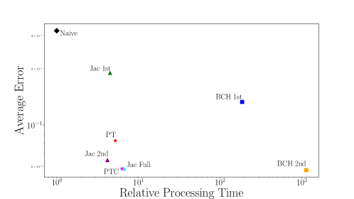
Figure 1: Comparative study of the average error (12) and the relative processing time of each fusion method. Relative processing time is measured as a ratio of algorithm run-time with respect to run-time for the naive fusion ($\diamond$) algorithm. “Jac Full($\triangle$)” refers to using the analytic form of the Jacobian of the transition functions. “Jac 1st($\triangle$)” and “Jac 2nd($\triangle$)” refer to first and second order Taylor approximations of the Jacobian. “PT($\star$)” refers to parallel transport and “PTC($\star$)” to parallel transport with curvature correction. “BCH 1st($\square$)” and “BCH 2nd($\square$)” refer to the Baker-Campbell-Hausdorff approximation methods proposed in [9].

In this paper we revisit the problem of stochastic fusion of concentrated Gaussians on Lie groups. We extend the concept of concentrated Gaussian to allow the mean of the Gaussian to be separate from the group element at which the exponential coordinates for the distribution are centred. This allows us to treat Gaussian fusion on the tangent space without requiring computationally expensive optimisation procedures. However, it is important to compensate for the change of coordinates associated with defining a covariance of a distribution at a non-zero mean in a given set of coordinates. We consider several approximations based on computing the exact Jacobian of the change of exponential coordinates map, first and second order Taylor’s expansions of the Jacobian, and parallel transport method. We also propose a novel method by using the parallel transport with curvature correction associated with the underlying geometry of the Lie group. This is particularly of interest since it can be implemented using only the matrix exponential function for which efficient implementations are readily available. We compare these five approximations with the BCH-based optimisation algorithms that are commonly used for fusion of concentrated Gaussians [9]. Preliminary results on $\mathbf{SO}(3)$ demonstrate that using parallel transport with curvature correction achieves similar accuracy to the state-of-the-art optimisation based algorithms at a fraction of the computational cost, as shown in Fig 1.

2 Preliminaries

2.1 General Lie groups

Let $\mathbf{G}$ be a general Lie group with dimension $n$, associated with Lie algebra $\mathfrak{g}$. Let $\mathrm{id}$ denote the identity element of $\mathbf{G}$. Given arbitrary $X,Y\in\mathbf{G}$, the left and right translations are denoted by $\textrm{L}_{X}$ and $\textrm{R}_{X}$, and are defined by

$$\textrm{L}_{X}(Y):=XY,\quad\textrm{R}_{X}(Y):=YX.$$

The Lie algebra $\mathfrak{g}$ is isomorphic to a vector space $\mathbb{R}^{n}$ with the same dimension. We use the wedge $(\cdot)^{\wedge}:\mathbb{R}^{n}\rightarrow\mathfrak{g}$ and vee $(\cdot)^{\vee}:\mathfrak{g}\rightarrow\mathbb{R}^{n}$ operators to map between the Lie algebra and vector space. The Adjoint map for the group $\mathbf{G}$, $\operatorname{Ad}_{X}:{\mathfrak{g}}\to{\mathfrak{g}}$ is defined by

$$\operatorname{Ad}_{X}[{{u}^{\wedge}}]=\mathrm{D}\textrm{L}_{X}\circ\mathrm{D}\textrm{R}_{X^{-1}}\left[{u}^{\wedge}\right],$$

for every $X\in\mathbf{G}$ and ${{u}^{\wedge}\in\mathfrak{g}}$, where $\mathrm{D}\textrm{L}_{X}$, and $\mathrm{D}\textrm{R}_{X}$ denote the differentials of the left, and right translation, respectively. Given particular wedge and vee maps, the Adjoint matrix is defined as the map ${\operatorname{Ad}_{X}^{\vee}:{\mathbb{R}^{n}}\to{\mathbb{R}^{n}}}$

$$\operatorname{Ad}_{X}^{\vee}u=\left(\operatorname{Ad}_{X}{{u}^{\wedge}}\right)^{\vee}.$$

The adjoint map for the Lie algebra $\operatorname{ad}_{{u}^{\wedge}}:{\mathfrak{g}}\to{\mathfrak{g}}$ is given by

$$\operatorname{ad}_{{u}^{\wedge}}{{v}^{\wedge}}=\left[{u}^{\wedge},{v}^{\wedge}\right],$$

and is equivalent to the Lie bracket. Given particular wedge and vee maps, the adjoint matrix $\operatorname{ad}_{u}^{\vee}:\mathbb{R}^{n}\to\mathbb{R}^{n}$ is defined to be

$$\operatorname{ad}_{u}^{\vee}v=\left(u^{\wedge}v^{\wedge}-v^{\wedge}u^{\wedge}\right)^{\vee}=\left[{u}^{\wedge},{v}^{\wedge}\right]^{\vee}.$$

Let $\exp_{\mathbf{G}}:\mathfrak{g}\to\mathbf{G}$ denote the exponential map from the Lie algebra element to the group element. For matrix Lie groups such as $\mathbf{SO}(3),\mathbf{SE}(3)$, this map is simply the matrix exponential. Let $\mathbf{G}^{\prime}\subset\mathbf{G}$ be the subset of $\mathbf{G}$ where the exponential map is invertible, one can then define the logarithm map $\log_{\mathbf{G}}:\mathbf{G}^{\prime}\to\mathfrak{g}$ and $\log_{\mathbf{G}}^{\vee}:\mathbf{G}^{\prime}\to\mathbb{R}^{n}$. For simplicity, we will suppress the wedge ‘$\wedge$’ operator in the exponential map throughout this paper.

Consider the directional derivative of $\exp_{\mathbf{G}}$ at a point $v\in\mathfrak{g}$ in the direction of $w\in\mathfrak{g}$, given by [12, Theorem 1.7]

$$\left.\frac{\mathrm{d}}{\mathrm{d}t}\exp_{\mathbf{G}}({u+tw})\right|_{t=0}=\mathrm{D}\textrm{L}_{\exp_{\mathbf{G}}(u)}\left\{\frac{\textrm{I}-\exp_{\mathbf{G}}({-\operatorname{ad}_{u}})}{\operatorname{ad}_{u}}(w)\right\}.$$

The differential $\mathrm{D}_{u}\exp_{\mathbf{G}}:\mathfrak{g}\to\mathrm{T}_{\exp_{\mathbf{G}}(u)}\mathbf{G}$ of $\exp_{\mathbf{G}}$ at $u$ can be derived immediately:

$$\mathrm{D}_{u}\exp_{\mathbf{G}}:=\mathrm{D}\textrm{L}_{\exp_{\mathbf{G}}(u)}\circ\frac{\textrm{I}-\exp({-\operatorname{ad}_{u}})}{\operatorname{ad}_{u}}.$$

This map is transcendental and is computed using asymptotic expansions for a general Lie group, although for specific Lie groups such as $\mathbf{SO}(3)$ and $\mathbf{SE}(3)$, algebraic forms exist in terms of known trigonometric transcendental functions $\sin$ and $\cos$ [13]. By identifying $\mathrm{T}_{\exp_{\mathbf{G}}(u)}\mathbf{G}$ with $\mathbb{R}^{n}$ via left trivialization and ‘$\vee$’ operator, one can define the left trivialised Jacobian map $J_{u}:\mathbb{R}^{n}\to\mathbb{R}^{n}$ as

$$J_{u}:=\mathrm{D}\textrm{L}_{\exp_{\mathbf{G}}(u)}^{-1}\mathrm{D}_{u}\exp_{\mathbf{G}}(u)=\frac{\textrm{I}-\exp(-\operatorname{ad}_{u}^{\vee})}{\operatorname{ad}_{u}^{\vee}},$$

for any $u\in\mathfrak{g}$ in the domain of $\exp_{\mathbf{G}}$. This expression corresponds to the right Jacobian in most literatures [13], where the left Jacobian can be obtained similarly by using a right trivialisation in the construction. The inverse Jacobian map is given by [hausdorffSymbolischeExponentialformelGruppentheorie2001]:

$$J_{u}^{-1}:=\sum_{k=0}^{\infty}\frac{B_{k}}{k!}\operatorname{ad}_{u}^{k},$$

with the Bernoulli numbers $B_{k}$.

2.2 Connection, curvature and parallel transport

For an arbitrary manifold, an affine connection is a geometric structure that is additional to the underlying differential structure. On Lie groups, however, there is a canonical connection (also known as the Cartan-Schouten (0)-connection), which is defined as the only affine connection that is left-invariant, torsion-free, and has geodesics given by the Lie exponential [14]. Other connections of interest in studying Lie groups include the Cartan-Schouten (-) and (+) connections [14], which share the same left-invariance and exponential geodesics, but have non-zero torsion that results in their parallel transport maps being given by left- and right-translation, respectively. In the case of compact Lie groups, such as $\mathbf{SO}(3)$, the canonical connection coincides with the Levi-Civita connection associated with the bi-invariant metric. In the rest of this paper, we will consider only the Cartan-Schouten (0)-connection as the default choice of affine connection on Lie groups.

Let $X,Y\in\mathfrak{X}(\mathbf{G})$ be two left-invariant vector fields on $\mathbf{G}$, corresponding to $x,y\in\mathfrak{g}$ respectively. For the (0)-connection, the covariant derivative $(\nabla_{X}Y)$ is given by

$$(\nabla_{X}Y)=\frac{1}{2}\left[X,Y\right].$$ (1)

The Riemann curvature tensor $\mathcal{R}:\mathfrak{X}(\mathbf{G})\times\mathfrak{X}(\mathbf{G})\times\mathfrak{X}(\mathbf{G})\to\mathfrak{X}(\mathbf{G})$ is defined by

$$\mathcal{R}(X,Y)Z=\nabla_{X}\nabla_{Y}Z-\nabla_{Y}\nabla_{X}Z-\nabla_{[X,Y]}Z.$$

Using the Jacobi identity of the Lie bracket, it is straightforward to verify that on a Lie group $\mathbf{G}$ with (0)-connection (1) the Riemann curvature tensor is given by

$$\mathcal{R}(X,Y)Z=-\frac{1}{4}\left[\left[X,Y\right],Z\right],$$ (2)

where $X,Y,Z\in\mathfrak{X}(\mathbf{G})$ are left-invariant vector fields.

For the (0)-connection, the curve $\exp_{\mathbf{G}}(tu)$ for $u\in\mathfrak{g}$ arbitrary, is a geodesic. Given $y\in\mathfrak{g}$, the parallel translation of $y$ along $\exp_{\mathbf{G}}(tu)$ is given by [15]

$$Y(t)=\mathrm{D}\mathrm{L}_{\exp_{\mathbf{G}}(tu)}\operatorname{Ad}_{\exp_{\mathbf{G}}(-\frac{t}{2}u)}(y)\in\mathrm{T}_{\exp_{\mathbf{G}}(tu)}\mathbf{G}.$$

By identifying $\mathrm{T}_{\exp_{\mathbf{G}}(tu)}\mathbf{G}$ with $\mathbb{R}^{n}$ via the left trivialisation and the ‘$\vee$’ operator, one can define the following left trivialised parallel transport map $\mathbf{P}_{u}:\mathbb{R}^{n}\to\mathbb{R}^{n}$

$$\mathbf{P}_{u}:=\operatorname{Ad}^{\vee}_{\exp_{\mathbf{G}}(-\frac{1}{2}u)}=\exp(-\frac{1}{2}\operatorname{ad}^{\vee}_{u})\in\mathbb{R}^{n\times n}.$$

3 Concentrated Gaussian Distribution

For a random variable $g\in\mathbf{G}$, the classical construction of concentrated Gaussian distribution on Lie group is given by

$$p(g;x,\Sigma)=\alpha\exp\left\{-\frac{1}{2}\left[\log^{\vee}_{\mathbf{G}}\left(x^{-1}g\right)\right]^{\top}\Sigma^{-1}\log^{\vee}_{\mathbf{G}}\left(x^{-1}g\right)\right\},$$

where $\alpha$ is the normalising factor. The parameters $x\in\mathbf{G}$, $\Sigma\in\mathbb{S}_{+}(n)$ are the group mean and covariance respectively, which are defined such that [13]

$$\int_{G}\log^{\vee}_{\mathbf{G}}\left(x^{-1}g\right)p(g)dg=\mathbf{0},$$

and

$$\Sigma=\int_{G}\left[\log^{\vee}_{\mathbf{G}}\left(x^{-1}g\right)\right]\left[\log^{\vee}_{\mathbf{G}}\left(x^{-1}g\right)\right]^{\top}p(g)dg.$$

This construction is equivalent to defining a random variable on $\mathbf{G}$ by

$$g=x\exp_{\mathbf{G}}(\epsilon),\qquad\epsilon\sim\mathbf{N}(0,\Sigma)$$

where $\epsilon$ is a random variable associated with a normal distribution on $\mathbb{R}^{n}$.

In more recent works [10][11], this concept was extended to allow offset mean in the Lie algebra

$$p(g;x,\mu,\Sigma)=$$ (3)

$$\alpha\exp\left\{-\frac{1}{2}\left[\log^{\vee}_{\mathbf{G}}\left(x^{-1}g\right)-\mu^{\vee}\right]^{\top}\Sigma^{-1}\left[\log^{\vee}_{\mathbf{G}}\left(x^{-1}g\right)-\mu^{\vee}\right]\right\},$$ (4)

where $x\in\mathbf{G}$ is termed the reference point, $\mu\in\mathfrak{g}$ is termed the mean. The extended concentrated Gaussian distribution is equivalent to defining a random variable

$$g=x\exp_{\mathbf{G}}(\epsilon),\qquad\epsilon\sim\mathbf{N}(\mu,\Sigma).$$

The extended concentrated Gaussian makes the role of the reference point as the origin of local coordinates on the group, as separate from the mean of the underlying distribution, clear. Both the classical and extended concentrated Gaussian distributions are approximations of the true distributions of a random variable on a Lie group after fusion. The key question is not whether they are the correct model, but rather how accurately they can represent real distributions.

3.1 Changing reference

The extended concentrated Gaussian (3) is introduced in order to provide a model to express Gaussians around a reference that does not coincide with their mean. A detailed formulation is provided in the following lemma.

Lemma 3.1.

Given an extended concentrated Gaussian distribution $p(g)=\mathbf{N}_{x_{1}}(\mu_{1},\Sigma_{1})$ on $\mathbf{G}$ and a point $x_{2}\in\mathbf{G}$ then the concentrated Gaussian $q(g)=\mathbf{N}_{x_{2}}(\mu_{2},\Sigma_{2})$ with parameters

$$\mu_{2}=\log^{\vee}_{\mathbf{G}}(x_{2}^{-1}x_{1}\exp_{\mathbf{G}}(\mu_{1}))$$ (5)

$$\Sigma_{2}=J_{\mu_{2}}^{-1}J_{\mu_{1}}\Sigma_{1}J_{\mu_{1}}^{\top}J_{\mu_{2}}^{-\top}$$ (6)

minimises the Kullback-Leibler divergence of $q(g)$ with respect to $p(g)$ up to second-order linearisation error.

Proof.

The Kullback-Leibler divergence between $p(g)$ and $q(g)$ is given by

$${\text{KL}}(p||q) =\mathbb{E}_{p}[\log(p)-\log(q)]$$

$$=C_{p}+\frac{n}{2}\log(2\pi)+\frac{1}{2}\log\det(\Sigma_{2})$$

$$+\frac{1}{2}\mathbb{E}_{p}[\left(\log_{\mathbf{G}}^{\vee}(x_{2}^{-1}g)-\mu_{2}\right)^{\top}\Sigma_{2}^{-1}\left(\log_{\mathbf{G}}^{\vee}(x_{2}^{-1}g)-\mu_{2}\right)],$$

where $C_{p}$ is the negative entropy of $p(g)$. The mean $\mu_{2}$ in (5) can be derived by assuming that

$$x_{1}\exp_{\mathbf{G}}(\mu_{1})=x_{2}\exp_{\mathbf{G}}(\mu_{2}).$$

Take the derivative of ${\text{KL}}(p||q)$ with respect to $\Sigma_{2}$ and the critical point is given by

$$\Sigma_{2}=\mathbb{E}_{p}[\left(\log_{\mathbf{G}}^{\vee}(x_{2}^{-1}g)-\mu_{2}\right)\left(\log_{\mathbf{G}}^{\vee}(x_{2}^{-1}g)-\mu_{2}\right)^{\top}].$$ (7)

Define $\phi_{1}:\mathbf{G}\to\mathbb{R}^{n}$ and $\phi_{2}:\mathbf{G}\to\mathbb{R}^{n}$ as

$$\phi_{1}(g):=\log_{\mathbf{G}}^{\vee}(x_{1}^{-1}g)-\mu_{1},$$

$$\phi_{2}(g):=\log_{\mathbf{G}}^{\vee}(x_{2}^{-1}g)-\mu_{2}.$$

For an arbitrary $g\in\mathbf{G}$ one has

$$\phi_{1}(g)=\log^{\vee}_{\mathbf{G}}(x_{1}^{-1}x_{2}\exp_{\mathbf{G}}(\phi_{2}(g)+\mu_{2}))-\mu_{1}$$ (8)

Taking the Taylor series of (8) at $\phi_{1}(g)=0_{n\times 1}$ up to first order yields:

$$\phi_{1}(g)\approx \mathrm{D}\log_{\mathbf{G}}^{\vee}(\exp_{\mathbf{G}}(\mu_{1}))\cdot\mathrm{D}\textrm{L}_{x_{1}^{-1}x_{2}}\cdot\mathrm{D}\exp_{\mathbf{G}}(\mu_{1})[\phi_{1}(g)]$$

$$= \mathrm{D}\log_{\mathbf{G}}^{\vee}(\exp_{\mathbf{G}}(\mu_{1}))\cdot\mathrm{D}\textrm{L}_{\exp_{\mathbf{G}}(\mu_{1})}\cdot\mathrm{D}\textrm{L}_{(x_{1}\exp_{\mathbf{G}}(\mu_{1}))^{-1}}\cdot$$

$$\quad\mathrm{D}\textrm{L}_{x_{2}\exp_{\mathbf{G}}(\mu_{2})}\cdot\mathrm{D}\textrm{L}_{\exp_{\mathbf{G}}(-\mu_{2})}\cdot\mathrm{D}\exp_{\mathbf{G}}(\mu_{2})\;[\phi_{2}(g)]$$

$$= \left(\mathrm{D}\textrm{L}_{\exp_{\mathbf{G}}(-\mu_{1})}\cdot\mathrm{D}\exp_{\mathbf{G}}(\mu_{1})\right)^{-1}\cdot$$

$$\quad\mathrm{D}\textrm{L}_{\exp_{\mathbf{G}}(-\mu_{2})}\cdot\mathrm{D}\exp_{\mathbf{G}}(\mu_{2})\;[\phi_{2}(g)]$$

$$= J_{\mu_{1}}^{-1}J_{\mu_{2}}\;[\phi_{2}(g)]$$

Substitute the result into (7):

$$\Sigma_{2} =\mathbb{E}_{p}[\phi_{2}(g)\phi_{2}(g)^{\top}]\approx J_{\mu_{2}}^{-1}J_{\mu_{1}}\Sigma_{1}J_{\mu_{1}}^{\top}J_{\mu_{2}}^{-\top},$$

which follows from the definition of $\Sigma_{1}=\mathbb{E}_{p}[\phi_{1}(g)\phi_{1}(g)^{\top}]$. ∎

Note that (5) is the exact coordinates of the mean in the new coordinates, and that (6) is the covariance conjugated by the Jacobian of the change-of-coordinates maps. That is, Lemma 3.1 can be thought of as transforming a Gaussian distribution under a non-linear change of coordinates.

Remark 3.2.

In the special case when $\mu_{1}=0$ or $\mu_{2}=0$, the covariance $\Sigma_{2}$ is given by

$$\Sigma_{2}=J_{\mu_{2}}^{-1}\Sigma_{1}J_{\mu_{2}}^{-\top}\quad\text{or}\quad\Sigma_{2}=J_{\mu_{1}}\Sigma_{1}J_{\mu_{1}}^{\top},$$

respectively. Both cases can happen in the fusion problem, as discussed in Sec 4.

3.2 Approximation with Curvature

The result in Lemma 3.1 relies on computing the linear map $J_{\mu}:\mathbb{R}^{n}\to\mathbb{R}^{n}$. However, as presented in Sec 2.1, this map is transcendental and except in special cases, must be computed using approximations of infinite power series. Analytic formulae in terms of classical trigonometric functions such as $\cos$ and $\sin$ exist for a limited range of Lie groups such as $\mathbf{SO}(3)$ and $\mathbf{SE}(3)$. In this section we propose a method to approximate the Jacobian using geometric structure of the Lie group.

The Jacobian is directly related to the differential of the exponential mapping on $\mathbf{G}$ which induces a Jacobi field. The following theorem is an application of [16, Theorem 3.1] on Lie groups.

Theorem 3.3.

Given $u\in\mathfrak{g}$, suppose $I\subseteq\mathbb{R}$ is an open interval containing 0. Define the geodesic $\gamma(t):=\exp_{\mathbf{G}}(tu)$ with $t\in I$. Choose an arbitrary $w\in\mathfrak{g}$, let $\mathcal{J}_{w}(t)$ be the Jacobi field along $\gamma(t)$ such that

$$\mathcal{J}_{w}(0)=0\qquad\text{and}\qquad\mathrm{D}_{t}\mathcal{J}_{w}(0)=w,$$

and it satisfies the Jacobi equation

$$\mathrm{D}^{2}_{t}\mathcal{J}_{w}(t)+\mathcal{R}(\mathcal{J}_{w}(t),\dot{\gamma}(t))\dot{\gamma}(t)=0,$$

then for $t\in I$, one has

$$\mathrm{D}_{tu}\exp_{\mathbf{G}}[w]=\frac{1}{t}\mathcal{J}_{w}(t).$$

This link with the Jacobi field provides an alternative method for computing approximations of the Jacobian when direct computation is not possible. Consider the map $(\mathbf{P}_{u})^{-1}\circ\mathrm{D}\textrm{L}_{\exp_{\mathbf{G}}(-u)}\circ\mathrm{D}_{u}\exp_{\mathbf{G}}:\mathfrak{g}\to\mathfrak{g}$, taking the Taylor expansion around $u=0$ yields [17, Theorem A.2.9]

$$(\mathbf{P}_{u})^{-1}\circ\mathrm{D}\textrm{L}_{\exp_{\mathbf{G}}(-u)}\circ\mathrm{D}_{u}\exp_{\mathbf{G}}[w]=w+\frac{1}{6}\mathcal{R}(u,w)u+\cdots.$$

Take the first order approximation,

$$J_{u}[w] =\mathrm{D}\textrm{L}_{\exp_{\mathbf{G}}(-u)}\circ\mathrm{D}_{u}\exp_{\mathbf{G}}[w]\approx\mathbf{P}_{u}(w+\frac{1}{6}\mathcal{R}(u,w)u)$$

$$=\mathbf{P}_{u}(w-\frac{1}{24}[[u,w],u])\quad\text{(Equation~{}\ref{eq:curvature_liegroup})}$$

$$=\mathbf{P}_{u}(w+\frac{1}{24}\operatorname{ad}_{u}^{2}(w))\quad\text{(Anti-symmetry of $[\cdot,\cdot]$)}$$

$$=\mathbf{P}_{u}(\textrm{I}+\frac{1}{24}\operatorname{ad}_{u}^{2})[w].\quad\text{(Bilinearity of $[\cdot,\cdot]$)}$$

Hence, the Jacobian $J_{u}$ can be approximated with

$$J_{u}\approx\mathbf{P}_{u}\>(\textrm{I}+\frac{1}{24}\operatorname{ad}_{u}^{2}),$$ (9)

where $\mathbf{P}_{u}$ models the change of tangent spaces via the parallel transport, and $\frac{1}{24}\mathbf{P}_{u}\circ\operatorname{ad}_{u}^{2}$ captures the curvature structure of the exponential map. We show that this approximation captures enough of the necessary information of the Jacobian of the exponential map to achieve good fusion results at a low computational cost.

4 Fusion on Lie groups

In this section, we propose a methodology to fuse multiple concentrated Gaussians on Lie groups. Consider the case that one has $n$ independent unbiased estimates $g\sim\mathbf{N}_{x_{i}}(0,\Sigma_{i})=p_{i}(g|x_{i},\Sigma_{i})$ for a random variable $g\in\mathbf{G}$. Each estimate is derived from independent data captured in the parameters $x_{i}\in\mathbf{G}$ and $\Sigma_{i}\in\mathbb{S}_{+}(n)$. We want to derive a fused estimate $g\sim\mathbf{N}_{x^{+}}(0,\Sigma^{+})=p(g|x_{1},\ldots,x_{n},\Sigma_{1},\ldots,\Sigma_{n})$ based on all the available data. In classical Gaussian fusion the solution is the product of the Gaussians and can be written as a Gaussian. However, the product of concentrated Gaussians is not a concentrated Gaussian and we must find the parameters $x^{+}\in\mathbf{G}$ and $\Sigma^{+}\in S_{+}(n)$ that best approximate the fused density. For simplicity, we only describe the case with two Gaussians, however, the extension to multiple Gaussians is direct.

The proposed methodology has 3 steps. The first step is to compute a reference point $\hat{x}\in\mathbf{G}$. In the second step, one of the approximation methods is used to express the independent concentrated Gaussians provided as data as extended concentrated Gaussians with respect to the chosen reference point. In these coordinates, classical Gaussian fusion is applied. The last step is to rewrite the fused extended concentrated Gaussian as a concentrated Gaussian around the group element corresponding to its mean.

Step 1: Reference

The goal of the first step of the methodology is to choose a reference point $\hat{x}\in\mathbf{G}$ as close to the true mean of the fused distribution as possible for the least reasonable computational cost. This point will be used as the reference point for the approximation of the independent concentrated Gaussians. The closer $\hat{x}$ is to the correct group-mean, the less approximation error will be incurred before the full fusion process is undertaken. However, spending excessive computation at this point is wasted since the independent concentrated Gaussians are defined at different points on the Lie group anyway and, as long as $\hat{x}$ is roughly central to the data, the particular choice of reference point will make little difference to the approximation.

Choice of a reference point is common to many of the standard fusion algorithms. In [11], and in general for Extended Kalman Filters (EKF), the authors choose $\hat{x}$ to be the reference for the prior distribution. More generally the reference $x_{1}$ of the first independent distribution could be chosen. In [9], an initial estimate $\hat{x}$ is derived by using the naive fusion method. Such choice can be iterated to achieve better accuracy at a higher computational cost, inspired by the iterated Kalman filter [18]. The authors in [8] use an optimization process to compute $\hat{x}$.

Naive Fusion: We use a simple algorithm to choose $\hat{x}$ that will also act as benchmark for the comparison study in Section 5. Consider $n$ independent estimates $\mathbf{N}_{x_{i}}(0,\Sigma_{i})$ for $i=1,\ldots,n$ of a random variable $g\in\mathbf{G}$. Consider exponential coordinates on the Lie group $\mathbf{G}$ around the origin. Approximate

$$\mathbf{N}_{x_{i}}(0,\Sigma_{i})\approx\mathbf{N}_{\mathrm{id}}(\log^{\vee}_{\mathbf{G}}(x_{i}),\Sigma_{i})$$

by an extended concentrated Gaussian in origin coordinates without any consideration of the change of coordinates on the covariance $\Sigma_{i}$. The distributions are now Gaussian in a single set of coordinates (the Lie algebra) and classical fusion is used to estimate the mean of the distribution

$$\hat{\mu}=\hat{\Sigma}\sum_{i=1}^{n}\Sigma_{i}^{-1}\log^{\vee}_{\mathbf{G}}(x_{i}),\quad\quad\quad\hat{\Sigma}=\left(\sum_{i=1}^{n}\Sigma_{i}^{-1}\right)^{-1}.$$

Set $\hat{x}=\exp_{\mathbf{G}}(\hat{\mu})$, the final distribution is $\mathbf{N}_{\hat{x}}(0,\hat{\Sigma})$. Note that it is possible to translate, by left multiplication, the naive fusion process to compute with respect to any arbitrary point on the Lie group. The identity is only used here for simplicity and to remove ambiguity in the comparisons.

Step 2: Fusion

Consider independent estimates $p(g|x_{i},\Sigma_{i})=\mathbf{N}_{x_{i}}(0,\Sigma_{i})$ for $i=1,\ldots,n$. We approximate each distribution by an extended concentrated Gaussian

$$p(g|x_{i},\Sigma_{i})\approx\mathbf{N}_{\hat{x}}(\mu_{i},\hat{\Sigma}_{i})$$

where $\mu_{i}=\log^{\vee}_{\mathbf{G}}(\hat{x}^{-1}x_{i})$ and $\hat{\Sigma}_{i}$ is given by the chosen approximation scheme.
Full Jacobian: The most direct approximation is provided by applying Lemma 3.1:

$$\hat{\Sigma}_{i}=J_{\mu_{i}}^{-1}\Sigma_{i}J_{\mu_{i}}^{-\top}$$ (10)

where an analytic expression for the inverse Jacobian $J_{\mu_{i}}^{-1}$ can be computed.
Approximate Jacobian: If no analytic version of the inverse Jacobian $J_{\mu_{i}}^{-1}$ is available, we can approximate this by Taylors expansions. We consider both first and second order approximations [19][8].
Parallel Transport and Curvature: As discussed in Section 3.2 the Jacobian can be approximated by parallel transport $J_{\mu_{i}}^{-1}\approx\mathbf{P}_{\mu_{i}}^{-1}$ or recalling (9) by parallel transport and curvature

$$J_{\mu_{i}}^{-1}\approx\left(\mathrm{I}+\frac{1}{24}\operatorname{ad}^{2}_{\mu_{i}}\right)^{-1}\mathbf{P}_{\mu_{i}}^{-1}\approx\left(\mathrm{I}-\frac{1}{24}\operatorname{ad}^{2}_{\mu_{i}}\right)\mathbf{P}_{\mu_{i}}^{-1}.$$

Fig 2 demonstrates the geometric transform process.

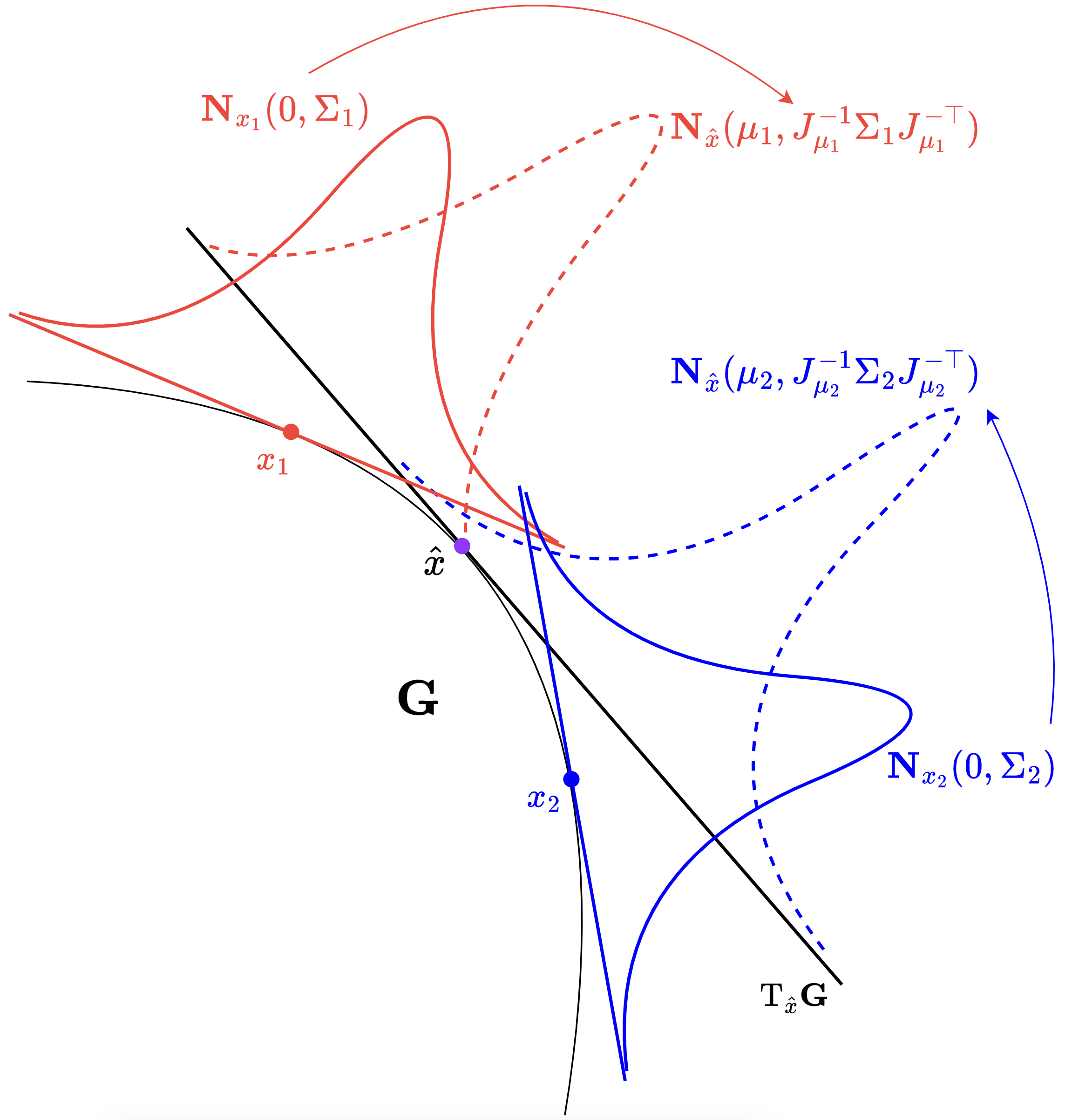
Figure 2: Demonstration of the geometric transform step. The distributions with solid red/blue lines are the original zero-mean concentrated Gaussians. The ones in dashed lines are the distributions after geometric transform.

Once the Gaussians are written in the same coordinates the distributions are fused using classical Gaussian fusion.

$$\Sigma_{\diamond}=\left(\sum_{i=1}^{n}\hat{\Sigma}_{i}^{-1}\right)^{-1},\quad\quad\quad\mu^{+}=\Sigma_{\diamond}\left(\sum_{i=1}^{n}\hat{\Sigma}_{i}^{-1}\mu_{i}\right).$$ (11)

Under the assumption that the distributions are independent, the fused estimate $(\mu^{+},\Sigma_{\diamond})$ is optimal with respect to multiple criteria such as the weighted least squares error, minimum covariance estimation error and maximum-likelihood estimation [20].

Step 3: Reset

The outcome of the fusion step is an extended concentrated Gaussian with non-zero mean $\mathbf{N}_{\hat{x}}(\mu^{+},\Sigma_{\diamond})$. If a concentrated Gaussian is required, which is the normal case for most filtering algorithms and estimators, then the extended concentrated Gaussian estimate must be transformed into a concentrated Gaussian around a new group mean. The problem is equivalent to finding $x_{+}\in\mathbf{G}$ and $\Sigma_{+}\in\mathbb{S}_{+}(n)$ such that

$$\mathbf{N}_{\hat{x}}(\mu^{+},\Sigma_{\diamond})\approx\mathbf{N}_{\hat{x}^{+}}(0,\Sigma^{+}).$$

This is also a direct application of Lemma 3.1. The new reference point $\hat{x}^{+}$ and the covariance $\Sigma^{+}$ are given by

$$\hat{x}^{+}=\hat{x}\;\exp_{\mathbf{G}}(\mu^{+}),$$

$$\Sigma^{+}=J_{\mu^{+}}\>\Sigma_{\diamond}\>J_{\mu^{+}}^{\top}.$$

The implementation of the reset will require either a full analytic version of the Jacobian to be computed, or an approximation to be used based on one of the methods discussed in Step 2. The new distribution $\mathbf{N}_{\hat{x}^{+}}(0,\Sigma^{+})$ is a zero-mean concentrated Gaussian.

5 Simulation

To numerically evaluate the proposed methods, we design the following simulation. For simplicity of the implementation, the special orthorgonal group $\mathbf{SO}(3)$ is chosen to be the Lie group of interest.

Following the experimental study in [9] we consider two zero-mean concentrated Gaussians on $\mathbf{SO}(3)$, denoted by $p_{1}(g)=\mathbf{N}_{\exp_{\mathbf{G}}(u_{1})}(0,\Sigma_{1})$ and $p_{2}(g)=\mathbf{N}_{\exp_{\mathbf{G}}(u_{2})}(0,\Sigma_{2})$. The parameters are chosen as

$$u_{1}=\frac{\gamma}{\sqrt{3}}\;[1.0,1.0,-1.0]\qquad u_{2}=\frac{\gamma}{\sqrt{2}}\;[1.0,-1.0,0.0]$$

and

$$\Sigma_{1}=\xi\begin{bmatrix}1.0&0&0\\ 0&0.75&0\\ 0&0&0.5\end{bmatrix}\quad\Sigma_{2}=\xi\begin{bmatrix}0.5&0&0\\ 0&1.0&0\\ 0&0&0.75\end{bmatrix}.$$

The scalars $\gamma$, and $\xi\in\mathbb{R}_{+}$ control the distance between means and the concentration of the covariance. As $\gamma$ increases and $\xi$ decreases the fusion becomes more non-linear.

To evaluate the performance, we use the cost function proposed in [9]:

$$E=\int_{G}\left|p^{+}(g)-\frac{p_{1}(g)p_{2}(g)}{\int_{G}p_{1}(h)p_{2}(h)\mathrm{d}h}\right|\mathrm{d}g$$ (12)

where $p^{+}(g)=\mathbf{N}_{\hat{x}^{+}}(0,\Sigma^{+})$. We implement by uniform sampling over a bounded domain on $\mathfrak{so}(3)$. This metric evaluates the difference between the approximated concentrated Gaussian distribution and the underlying ‘fused density’.

We run the simulation with different combinations of $\gamma$ and $\xi$, where both parameters are varied from 0.1 to 1.8. Each result is averaged over a Monte Carlo simulation with 500 runs where the covariance matrices are rotated by random rotation matrices.

5.1 Different approximation methods

In this section, we present the main results demonstrating the performance of different approximation methods. The Naive method is implemented directly. Approximate Jacobian and parallel transport methods proposed in Section 4 are implemented as described with the same Jacobian approximation used in the reset. For comparison, we include the BCH-based methods (first and second order) proposed in [9]. We use the standard minimizer in the SciPy library to implement the optimisations required by these methods. The BCH methods do not require reset. All methods use the same naive posterior as the initial guess $\hat{x}$.

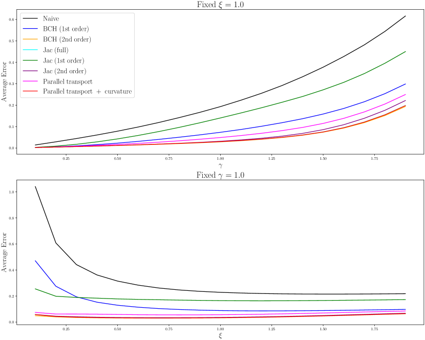
Figure 3: Estimation error using different approximation methods with fixed $\gamma=1.0$ or $\xi=1.0$.

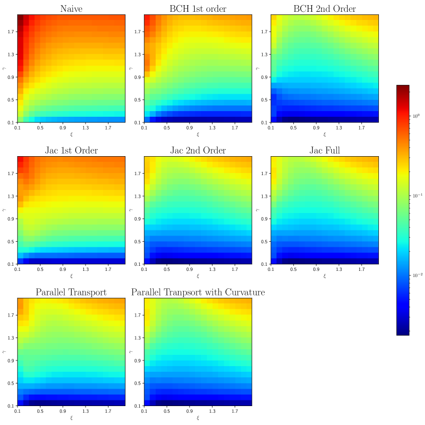
Figure 4: Heatmaps showing the estimation error with different approximation methods.

Figure 1 plots the average error and relative processing time of each method, averaged over all the parameter values of $\xi$ and $\gamma$. To account for the dependence on the computer hardware used, we show the ratio of processing time for each algorithm as compared to the naive fusion. Since all algorithms require the naive fusion as a first estimate of the reference point, this ratio is always greater than one. In Fig 3, we present the average estimation error of different methods when either $\gamma$ or $\xi$ is fixed at 1.0 and the other parameter changes. Fig 4 shows how the error in each method varies with different combinations of the parameters $\gamma$ and $\xi$.

In general, the naive fusion method has the worst performance among all the methods, as expected. The first order methods (BCH 1st order and Jac 1st order) perform marginally better but still show significant approximation error, and especially so for large values of $\gamma$. Interestingly, the first order BCH method is also highly sensitive to small $\xi$. The parallel transport method can also be thought of as a first order method. It performs better than the other first order methods but incurs more performance error than the remaining methods.

The last four methods all use higher order information in the Jacobian approximation (higher order terms in the BCH expansion for the BCH method). Clearly, the full Jacobian outperforms the second order Taylor approximation, although the difference is less significant than the difference with the first order Jacobian. The full order Jacobian, parallel transport with curvature (PTC) and BCH 2nd achieve very similar average error. The combination of parallel transport and curvature clearly captures the major nonlinearities in the full Jacobian without requiring computation of the analytic form of the Jacobian. This is particularly of interest for Lie groups where a closed-form expression of the Jacobian is not available; the parallel transport only requires computing a matrix exponential, which has an efficient implementation in many linear algebra programming libraries. The second order BCH method achieves the lowest average error in our simulations. However, the BCH-based methods do not admit closed-form solutions and can only be implemented with an optimization process, resulting in much higher computational cost ($>100$ times greater than the PTC method), as shown in Fig 1. These results are based on applying a standard optimisation routine, however, even a tailored optimisation algorithm is unlikely to significantly reduce this computational discrepancy.

5.2 Choice of the initial mean $\hat{x}$

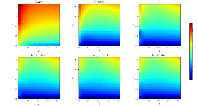
Figure 5: Heatmaps showing the estimation error with different choice of initial mean $\hat{x}$.

In this simulation, we run different implementations, all using the full Jacobian mapping but with different choices of the initial guess $\hat{x}$ in the geometric transform step, as discussed in Sec 4. The methods being compared are using identity, $x_{1}$ or iterated posterior as the initial guess, respectively. The naive fusion algorithm is also implemented as a baseline.

Fig 5 shows the heatmaps of the estimation error in different implementations. As shown in the figures, using the naive posterior clearly outperforms all the other methods, while having more iterations does not further improve the performance significantly.

5.3 Effect of reset step

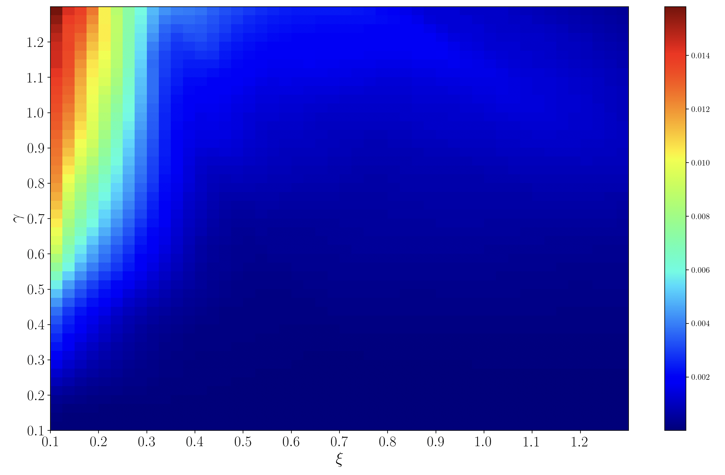
Figure 6: Heatmap showing the difference between fusion with reset and without reset, $\Delta E:=E_{\text{NoReset}}-E_{\text{Reset}}$

In the last simulation, we run a comparison between two implementations, one with the reset step as discussed in Sec 4 and one without reset. Both candidates are running the algorithm using the full Jacobian mapping. Same as the previous examples, the experiment is run across a range of $\gamma$ and $\xi$ parameters. The difference is computed by $\Delta E:=E_{\text{NoReset}}-E_{\text{Reset}}$.

As shown in Fig 6, the proposed reset step, although not significantly, improves the fusion accuracy by obtaining a more accurate covariance estimate. Similar to the previous examples, the modification tends to have larger impact when the means are sparsely distributed ($\gamma$ large) and the covariance is small ($\xi$ small). The difference is insignificant in a one-step simulation, however, in a recursive example it will have a larger difference in the long term due to the error accumulating.

6 Conclusion

This paper presents a general design methodology for fusion of independent concentrated Gaussian distributions on Lie groups from a geometric perspective. It is shown that by transforming a collection of distributions into a single, unified set of coordinates, the fusion problem can be solved using the same methodology as in the Euclidean case. In the simulation, we present the effectiveness of the different methods proposed, and, in particular, show that the parallel transport with curvature correction can achieve good performance at a low computational cost, while using only functions that are available in most linear algebra libraries.

References

- [1] S. Särkkä and L. Svensson, Bayesian Filtering and Smoothing. Cambridge University Press, May 2023.
- [2] R. E. Kalman, “A New Approach to Linear Filtering and Prediction Problems,” Journal of Basic Engineering, vol. 82, no. 1, pp. 35–45, Mar. 1960.
- [3] N. J. Gordon, D. J. Salmond, and A. F. M. Smith, “Novel approach to nonlinear/non-Gaussian Bayesian state estimation,” IEE Proceedings F (Radar and Signal Processing), vol. 140, no. 2, pp. 107–113, Apr. 1993.
- [4] H. E. Rauch, F. Tung, and C. T. Striebel, “Maximum likelihood estimates of linear dynamic systems,” AIAA Journal, vol. 3, no. 8, pp. 1445–1450, 1965.
- [5] A. Barrau and S. Bonnabel, “The Invariant Extended Kalman Filter as a Stable Observer,” IEEE Transactions on Automatic Control, vol. 62, no. 4, pp. 1797–1812, Apr. 2017.
- [6] R. Mahony, P. van Goor, and T. Hamel, “Observer Design for Nonlinear Systems with Equivariance,” Annual Review of Control, Robotics, and Autonomous Systems, vol. 5, no. 1, pp. 221–252, May 2022.
- [7] G. Bourmaud, R. Mégret, A. Giremus, and Y. Berthoumieu, “From Intrinsic Optimization to Iterated Extended Kalman Filtering on Lie Groups,” Journal of Mathematical Imaging and Vision, vol. 55, no. 3, pp. 284–303, Jul. 2016.
- [8] T. D. Barfoot and P. T. Furgale, “Associating Uncertainty With Three-Dimensional Poses for Use in Estimation Problems,” IEEE Transactions on Robotics, vol. 30, no. 3, pp. 679–693, Jun. 2014.
- [9] K. C. Wolfe and M. Mashner, “Bayesian Fusion on Lie Groups,” Journal of Algebraic Statistics, vol. 2, no. 1, Apr. 2011.
- [10] Y. Ge, P. van Goor, and R. Mahony, “Equivariant Filter Design for Discrete-time Systems,” in 2022 IEEE 61st Conference on Decision and Control (CDC), Dec. 2022, pp. 1243–1250.
- [11] Y. Ge, P. Van Goor, and R. Mahony, “A Note on the Extended Kalman Filter on a Manifold,” in 2023 62nd IEEE Conference on Decision and Control (CDC), Dec. 2023, pp. 7687–7694.
- [12] S. Helgason, Differential Geometry, Lie Groups, and Symmetric Spaces. Academic Press, Feb. 1979.
- [13] G. S. Chirikjian, Stochastic Models, Information Theory, and Lie Groups, Volume 2: Analytic Methods and Modern Applications. Springer Science & Business Media, Nov. 2011.
- [14] S. Kobayashi and K. Nomizu, Foundations of Differential Geometry, Volume 2. John Wiley & Sons, Feb. 1996.
- [15] S. T. Smith, Geometric Optimization Methods for Adaptive Filtering. Harvard University, 1993.
- [16] S. Lang, Fundamentals of Differential Geometry. Springer Science & Business Media, Dec. 2012.
- [17] S. Waldmann, “Geometric wave equations,” arXiv preprint arXiv:1208.4706, 2012.
- [18] H. W. Sorenson, “Kalman Filtering Techniques,” in Advances in Control Systems, C. T. Leondes, Ed. Elsevier, Jan. 1966, vol. 3, pp. 219–292.
- [19] A. W. Long, K. C. Wolfe, M. J. Mashner, G. S. Chirikjian et al., “The banana distribution is Gaussian: A localization study with exponential coordinates,” Robotics: Science and Systems VIII, vol. 265, p. 1, 2013.
- [20] F. C. Schweppe, Uncertain Dynamic Systems. Prentice-Hall, 1973.