Transient Waiting Time Distributions in Small Call Centres with Skills-Based Routing

Abstract

Many call centres are subject to service level agreements that stipulate that they must achieve targets in terms of the proportion of calls that are answered within a specified time. In order to manage a centre so that targets like these are met, we need to have a method of calculating the waiting time distributions experienced by customers. In this paper, we provide such a method for small call centres that employ skills-based routing. We first build the methodology for the single-skill case and then extend it to a multi-skill case. We model the call centre system as a continuous-time Markov chain and then make use of the Laplace transform to calculate the relevant quantities. We later demonstrate the use of this method to find the optimal routing policy in a certain class of policies.

Keywords: Call centre, queueing, transient, waiting time.

Acknowledgements. This research was partially funded by the Australian Government through the Australian Research Council Industrial Transformation Training Centre in Optimisation Technologies, Integrated Methodologies, and Applications (OPTIMA), Project ID IC200100009.

This research was partially funded by Probe CX.

This research was supported by The University of Melbourne’s Research Computing Services and the Petascale Campus Initiative.

1 Introduction

The term call centre is commonly used to describe a telephone-based human-service operation. A call centre provides tele-services, namely services in which customers and service agents are remote from each other [17].

It is common for specialist call centre providers to manage centres for client companies, in which case the provider is usually responsible for meeting the provisions of a service level agreement. For instance, they may be required to answer at least $90\%$ of all calls within $20$ seconds and have no more than $3\%$ abandonments measured over a month. The cost of human resources typically constitutes more than $60\%$ of the overall operating expenses of a telephone service centre ([13], [6]). Hence, a reasonable objective for a call centre service provider is to minimise staffing requirements while fulfilling its agreed targets. In a previous paper [16], we discussed how to calculate the expected number of abandonments and the expected total waiting time in $(0,t)$. In this paper, we extend this analysis to calculate the waiting time distributions of the customers. This requires first modelling the waiting times of customers, conditional on the state that they observe on arrival and then taking expectations over the possible states.

In most call centres, customer inquiries are categorised based on their complexity. Likewise, agents are categorised according to their skill set. An arriving caller is first directed to an automatic Interactive Voice Response (IVR) system, which asks questions that enable it to classify what type of query the caller has. The task is then to allocate the call to a suitable agent. Since some agents have multiple skills that enable them to deal with more than one type of enquiry, this is not a straightforward decision and there is an opportunity for a call centre to increase its efficiency by making these decisions in an optimal manner. The rules governing the assignment of incoming calls are termed policies here, and different policies can lead to variations in the call centre’s performance.

There are many papers on the waiting time distributions of customers for queueing systems. Stationary waiting time distributions have been calculated in [9] for the bulk service queues, in [8] for a multi-server priority queueing system, in [18] for the $M/M/1$ queue under a general bulk service rule, in [21] for queues with phase-type servers and queues that can be represented as a quasi-birth-and-death process, in [11] for the random order service $M/M/1$ queue, in [12] for the $M/D/c$ queue, in [23] for the accumulating priority queue, in [20], [1], and [15] for the $GI/G/1$ queue using different formulas and in [10] for the preemptive accumulating priority queue with a single server.

There is a smaller number of papers that address the transient waiting time distribution. The author of [19] obtained an expression for the Laplace–Stieltjes transform of the transition probabilities and the generating function of the queue length for a general class of bulk queues. In [4], the author addressed the standard deviation and covariance function of transient waiting time distributions for the $GI/G/1$ queue. An algorithm to find the probability of being in state $k$ at time $t$ for Markovian queues and its application to the $M/M/1$ queue was given in [14]. Lower bounds for the tails of the steady state and transient waiting time distributions for the $M/GI/s$ queue were given in [26]. The authors of [25] proposed a method to approximate the transient performance measures of a discrete time queueing system via a steady state analysis. The transient probabilities of the queue size for the $M/M/c$ queue with balking and reneging were calculated in [22]. The expressions for the time dependent probabilities and other performance measures for the $M/M/1$ queue were obtained in [24] and [3] under different conditions.

In this paper, we develop a method to calculate the waiting time distributions in call centres that can be modelled as Markov chains under a transient setting without using any asymptotic regimes. It is important to use the transient setting because in a call centre, the call arrival rate changes throughout the day and the number of agents also changes with changes in shifts, hence the initial state of the system cannot be ignored while calculating performance measures.

Our study has been motivated by a problem brought to us by an industry partner that manages call centres for its clients. The particular centre that the industry partner was interested in is reasonably small, with around a dozen agents in total. Furthermore, there are four levels of agents of increasing expertise who are required to handle four levels of queries of increasing complexity. Agents at level $j$ are able to handle queries from all levels less than or equal to $j$.

In [16], we calculated the expected values of some performance measures for such a call centre when some defined call allocation policies are used. In this paper, we aim to extend this study by calculating the distribution function of the waiting time of customers which, as we observed above, is needed for meeting measures that are often inserted into service level agreements. It is more difficult to calculate distribution functions than expectations, especially for more than one type of caller. Depending on the policy, a customer may jump in front of other customers, hence the waiting time of a customer can be affected by other customers that arrive later.

We will focus on reservation policies. Under this class of policies, if there is an arrival of a level $j-1$ caller, we first try to assign that call to a level $j-1$ agent and if they all are busy, we check the number of level $j$ agents available, and if this number is greater than or equal to a certain number $n_{j}$ (which we define later in Subsection 4.1), we assign the call to one of the available level $j$ agents. Otherwise, the caller has to wait in the queue.

When a service is completed by a level $j$ agent, that level $j$ agent will first look for level $j$ calls and answer them in first-come-first-served (FCFS) order, and if no level $j$ calls are in waiting but level $j-1$ calls are in waiting, then they will take the first level $j-1$ call in the queue if the number of level $j$ agents available is at least $n_{j}$. This implies that customers at the same level are served according to an FCFS discipline, but this does not apply across levels.

We model the system as a continuous-time Markov chain (CTMC), assuming that the calls are arriving according to a Poisson process, and the service and abandonment times are exponentially distributed. The method we will use here was introduced in [7].

We start by illustrating the method for a simple case where there is one type of caller and one class of agent in Section 2. In Section 3 we plot the waiting time distribution function for a numerical example. In Section 4 we develop the method for four types of callers, and in Section 5 we give a numerical example utilising the method to find the optimal number of agents to be reserved at each level such that the percentage of callers served within $20$ seconds is maximised for a given set of parameters. We conclude the paper and give future directions in Section 6.

2 A single level

Assume that there are $k$ agents and $\ell$ telephone lines in total with $\ell\geq k$. A caller is lost if they call when all the lines are busy.

We model the system with a CTMC $X(t)$ with state space $S_{1}=\{0,1,\dots,\ell\}$, each state denoting the number of callers in the system. Let $\lambda$ be the arrival rate of calls requiring agents’ assistance, $\mu$ be the service rate and $\theta$ be the abandonment rate (see Figure 1).

Figure 1: Flowchart of a call in a call centre

For $i\in\{0,1,\dots,\ell-1\}$, there is a transition from $i$ to $i+1$ in the case of an arrival and for $i\in\{1,2,\dots,\ell\}$, there is a transition from $i$ to $i-1$ in the case of a service or an abandonment. The arrival rate is equal to $\lambda$ if $i<\ell$, otherwise, the caller is blocked. Let $\lambda^{i}=\lambda\mathbbm{1}_{i<\ell}$. The service rate is equal to $i\mu$ if $i\leq k$ and is equal to $k\mu$ otherwise. Let $\mu^{i}=\min(i,k)\mu$. Similarly, the abandonment rate is equal to $0$ if there is no one in the queue ($i\leq k$) and is equal to $(i-k)\theta$ if there are $i-k$ callers waiting ($i>k$). Let $\theta^{i}=\max(0,i-k)\theta$. Hence, the transition rates are

$$q_{i,i+1}=\lambda^{i}$$ (1)

$$q_{i,i-1}=\mu^{i}+\theta^{i}.$$ (2)

2.1 Expected time spent in each state during the time interval $(0,t)$

For $a\in\{0,1,\dots,\ell\}$ and $t>0$, let $\mathbf{v}_{a}(t)$ be a vector of length $\ell+1$ with the $i^{th}$ entry denoting the expected time spent by the system in state $i$ during the time interval $(0,t)$ given that the system is in state $a$ at time $0$. Let $\mathbf{v}_{a}(t|x)$ be the same quantity as $\mathbf{v}_{a}(t)$ conditional on the fact that $x$ is the first time that the system leaves state $a$.

Let $\mathbf{e}_{a}$ be a unit vector of length $\ell+1$ with a $1$ in the $a$^th entry for $a\in\{0,1,\dots,\ell\}$. Then for $a\in\{0,1,\dots,\ell\}$

$$\mathbf{v}_{a}(t|x)=\begin{cases}t\mathbf{e}_{a}&t<x\\[8.61108pt] x\mathbf{e}_{a}+\dfrac{\lambda^{a}\mathbf{v}_{a+1}(t-x)+(\mu^{a}+\theta^{a})\mathbf{v}_{a-1}(t-x)}{\lambda^{a}+\mu^{a}+\theta^{a}}&t\geq x.\end{cases}$$ (3)

This is because $t<x$ implies that the system remains in state $a$ for the entire duration of $(0,t)$, and $t>x$ implies that the system remains in state $a$ until time $x$ and then transitions to another state according to the transition rates.

As the model is a Markov chain and $x$ is exponentially distributed with rate $\lambda^{a}+\mu^{a}+\theta^{a}$, we can remove the conditioning with respect to $x$ by integrating $\mathbf{v}_{a}(t|x)$ to derive an expression for $\mathbf{v}_{a}(t)$, we have

$$\begin{split}\mathbf{v}_{a}(t)=&\int_{0}^{t}\left(x\mathbf{e}_{a}+\dfrac{\lambda^{a}\mathbf{v}_{a+1}(t-x)+(\mu^{a}+\theta^{a})\mathbf{v}_{a-1}(t-x)}{\lambda^{a}+\mu^{a}+\theta^{a}}\right)dF_{a}(x)+\int_{t}^{\infty}t\mathbf{e}_{a}dF_{a}(x)\\[4.30554pt] =&\int_{0}^{t}(\lambda^{a}\mathbf{v}_{a+1}(t-x)+(\mu^{a}+\theta^{a})\mathbf{v}_{a-1}(t-x))e^{-(\mu^{a}+\theta^{a}+\lambda^{a})x}dx\\[4.30554pt] &+\dfrac{(1-e^{-(\mu^{a}+\theta^{a}+\lambda^{a})t})}{(\mu^{a}+\theta^{a}+\lambda^{a})}\mathbf{e}_{a}.\end{split}$$

It follows that the Laplace transforms of $\mathbf{v}_{a}(t)$, denoted by $\mathbf{\tilde{v}}_{a}(s)$, satisfy the equations

$$\mathbf{\tilde{v}}_{a}(s)=\dfrac{\mathbf{e}_{a}/s+\lambda^{a}\mathbf{\tilde{v}}_{a+1}(s)+(\mu^{a}+\theta^{a})\mathbf{\tilde{v}}_{a-1}(s)}{\lambda^{a}+\mu^{a}+\theta^{a}+s}$$ (4)

with $\mathbf{\tilde{v}}_{a}(s)=\mathbf{0}$ for $a\notin\{0,1,\dots,\ell\}$.

For a given set of parameters, we can solve these equations numerically and then invert them using the Euler method discussed in [2] to obtain $\mathbf{{v}}_{a}(t)$.

2.2 Distribution of the state of the system observed by a uniformly distributed arrival in $(0,t)$

The $i^{\text{th}}$ component of the vector $\mathbf{v}_{a}(t)$ contains the expected amount of time that there are exactly $i$ customers in the system during $(0,t)$. If follows that $\mathbf{v}_{a}(t)/t$ is a vector whose $i^{\text{th}}$ component is the expected proportion of time in $(0,t)$ that there are $i$ customers in the system.

Assume that a tagged customer arrives to the system at a uniformly distributed time $T$ in $(0,t)$. Then the $i^{\text{th}}$ component of $\mathbf{v}_{a}(t)/t$ is the expected value of the indicator random variable that the customer finds the system in state $i$. This is, in turn, the probability $r_{a,i}(t)$ that the customer finds the system in state $i$.

We will use these probabilities to calculate the waiting time distributions but they can also be used to calculate other important measures for call centres such as the average queue size or the queue size distribution at a uniformly distributed point in $(0,t)$. For example, we might be interested in finding the minimum number of agents required such that the probability of the queue size at a uniformly distributed arrival time being greater than a certain threshold value is less than $0.05$.

2.3 The waiting time distribution of a caller who arrives with $i$ customers in front of them

We consider a tagged customer who arrives at a uniformly distributed time $T$ in the interval $(0,t)$. Let $W$ be the time until the customer is served, with $W=\infty$ if the customer abandons before they are served.

For $i\in\{0,1,\ldots,\ell-1\}$, we discuss how to calculate the waiting time distribution

$$\Xi_{i}(y)=P(W\leq y|X(T)=i+1),$$ (5)

conditional on the tagged customer finding $i$ customers in front of them when they arrive. Note that, because customers are served in an FCFS order in this model, the waiting time of the tagged caller is not affected by the arrivals of any future callers.

If a caller arrives when there are less than $k$ callers in the system, they can be served immediately. It follows that for $i<k$ and any $y\geq 0$,

$$\Xi_{i}(y)=1.$$ (6)

To derive the waiting time distribution $\Xi_{i}$ when $i\geq k$, we introduce a Markov chain $\chi_{t}$ with state space $\{k,\ldots,i\}$ whose state at time $t$ is the number of customers in front of the tagged caller at that time. Because this number cannot increase in the single-level model, $\chi_{t}$ is a pure death process. This will not be the case in the multilevel model that we consider in Section 4. In both cases, however, the time until the tagged customer enters service is the time until a finite state Markov chain is absorbed and hence it has a phase-type distribution. The details are discussed below.

For $i\geq k$, let $\Xi_{i}(y|z)$ be the same quantity as $\Xi_{i}(y)$ conditional on the fact that $z$ is the first time that $\chi_{t}$ leaves state $i$. If a caller arrives when all agents are busy and there is no change in the state until time $y$, the probability of being served within $y$ time units is $0$. If a caller arrives when all agents are busy and the first change in the state takes place within $y$ time units, there are two possibilities - the first is that the tagged caller has abandoned the queue before time $y$ in which case the probability of being served within $y$ time units is $0$; and the second possibility is that the caller has not abandoned (with probability given by the bracketed term in Equation (7)) and that there is a transition from state $i$ to $i-1$ (either one of the callers in front has abandoned or been served).

Hence, for $i\geq k$ and $y\geq 0$,

$$\Xi_{i}(y|z)=\begin{cases}0&y<z\\ \left(1-\dfrac{\theta}{\mu_{i+1}+\theta_{i+1}}\right)\Xi_{i-1}(y-z)&y\geq z.\end{cases}$$ (7)

Now, similar to Subsection 2.1, we can write an expression for $\Xi_{i}(y)$ and then take its Laplace transform. For $i\in\{0,1,\dots,\ell-1\}$, the Laplace transforms, $\tilde{\Xi}_{i}(s)$ satisfy

$$\tilde{\Xi}_{i}(s)=\begin{cases}\dfrac{1}{s}&i<k\\[8.61108pt] \left(1-\dfrac{\theta}{\mu_{i+1}+\theta_{i+1}}\right)\dfrac{\mu_{i+1}+\theta_{i+1}}{\mu_{i+1}+\theta_{i+1}+s}\tilde{\Xi}_{i-1}(s)&i\geq k\end{cases}$$ (8)

so that,

$$\begin{split}\tilde{\Xi}_{i}(s)&=\prod_{j=k}^{i}\dfrac{\mu_{j+1}+\theta_{j+1}-{\theta}}{s(\mu_{j+1}+\theta_{j+1}+s)}+\dfrac{\mathbbm{1}_{i<k}}{s}\\ &=\prod_{j=k}^{i}\dfrac{k\mu+(j-k)\theta}{s(k\mu+(j+1-k)\theta+s)}+\dfrac{\mathbbm{1}_{i<k}}{s}.\end{split}$$ (9)

Again, we can solve these equations and then invert them using the Euler method.

2.4 The unconditional waiting time distribution

By the PASTA property, the probability of the system being in a particular state at a uniformly-distributed point in the interval $(0,t)$ is equal to the probability of the system being in that state when a caller arrives [5]. We calculated these probabilities in Subsection 2.2. In Subsection 2.3, we calculated the probability of a caller being served within $y$ time units given the state of the system when the caller arrives.

Using these two quantities, we can calculate the probability $P_{a}(y,t)=P(W\leq y|X(0)=a)$ that a caller arriving during the interval $(0,t)$ is served within $y$ time units given that $a$ is the initial state at time $0$. Since the arrivals follow a Poisson process, given the total number of arrivals in an interval, the arrivals are independently and uniformly distributed over the interval. Using the notation from Subsections 2.2 and 2.3,

$$P_{a}(y,t)=\sum_{i=0}^{\ell-1}\Xi_{i}(y)r_{a,i}(t).$$ (10)

2.5 The end effect

It is important to note that Equation (10) gives an expression for the waiting time distributions of customers who arrive at a uniformly distributed time in $(0,t)$ (when there are initially $a$ customers in the system). This is different from the waiting time distribution of customers served in $(0,t)$ because the ‘fate’ of some of these customers might not be decided before time $t$. For example, there could be customers who arrive in $(t-y,t)$ who are still waiting at time $t$. These customers might or might not be served within time $y$ of their arrival.

3 Example

Figure 2 shows the graph of the distribution function of the waiting time of customers arriving in the next $60$ minutes for $\lambda=1,\mu=1/3,\theta=1/4,k=5$ and $\ell=20$. Let the initial state be $0$. For this set of parameters, the probability of being served within $0.5$ minutes is $0.8870$. The value of the function is equal to $0.9651$ for all values of $y$ from $5.6$ to $20$ (when rounded off), suggesting that $0.9651$ is the probability that a customer is not lost or does not abandon, and that the probability of a customer waiting longer than $5.6$ minutes to be served is very low. The probability of a customer being blocked is same as finding the system in state $\ell$, denoted by $r_{0,\ell}(t)$, which in this case is of the order $10^{-10}$. Hence, the probability that a customer who arrives in $(0,t)$ will eventually abandon is $0.0349$.

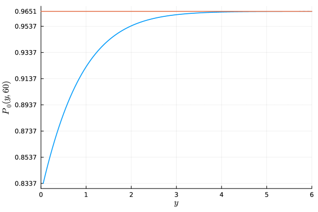
Figure 2: Graph of $P_{0}(y,60)$ versus $y$ for parameter values $\lambda=1,\mu=1/3,\theta=1/4,k=5$ and $\ell=20$

The expected number of abandonments in $(0,t)$ calculated using Subsection $2.2$ of [16] and then divided by the expected number of arrivals in $(0,t)$, for the above set of parameters, is equal to $0.0344$. This is slightly less than the probability of abandonment calculated using the method above. The reason is that the two quantities are different, the first is the expected number of abandonments amongst customers who arrive in $(0,t)$, while the second is the expected number of abandonments that occur in $(0,t)$.

The abandonments from existing customers is included in the method described in [16] but not in the method used in the example above which includes only those abandonments that arise from the arrivals during $(0,t)$. If we start with an empty system at the start of our time interval as in the example above, all the abandonments taking place during $(0,t)$ are arising from the arrivals in $(0,t)$. Hence, these abandonments will be counted in both methods. However, the example also counts abandonments of those customers that arrived during $(0,t)$ but abandoned after $t$. This is not included in the method described in [16].

If we start with a high number of customers at time $0$, for example, with $a=10$, the expected proportion of abandonments calculated using the method in [16] is $0.0858$, whereas the probability of abandonment using the method above is $0.0617$. This is because we are starting with a high number of customers in the beginning and many abandonments during $(0,t)$ arise from those existing customers.

4 Four levels

Now, we will modify the method above to calculate the waiting time distributions when there are four types of calls and four classes of agents, which is equal to the number of levels our partner call centre uses.

4.1 Policy and parameters

For $j\in\{1,2,3,4\}$, let $\lambda_{j}$ be the arrival rate of level $j$ callers, $\theta_{j}$ be the abandonment rate of level $j$ callers, $k_{j}$ be the total number of level $j$ agents, $\mu_{j}$ be the service rate when level $j$ callers are served by level $j$ agents, and for $j\in\{1,2,3\}$, $\mu_{j}^{\prime}$ be the service rate when level $j$ callers are served by level $j+1$ agents. Note that this notation is different from the notation introduced in the single level case as they denote different quantities. Let $\ell$ be the total capacity of the system shared by all callers regardless of their level. The probability that an arriving caller is of level $j$ is given by $\lambda_{j}/\Sigma_{j=1}^{4}\lambda_{j}$ for $j\in\{1,2,3,4\}$.

We characterise the reservation policy through a reservation vector $\mathbf{n}=(n_{2},n_{3},n_{4})$ where $n_{j}$ denotes the number of level $j$ agents reserved to answer only level $j$ calls.

Because the number of reserved agents has to be less than the total number of agents at that level, for $j\in\{2,3,4\}$, $n_{j}\in\{0,1,\dots,k_{j}\}$.

4.2 Distribution of the state of the system during the interval $(0,t)$

4.2.1 State space

We use the same state space as [16] with a generic state denoted by $(a,a_{1},b,b_{1},c,c_{1},d)$, where $a,b,c$ and $d$ are the total numbers of level $1$, $2$, $3$ and $4$ callers in the system, and $a_{1},b_{1}$ and $c_{1}$ are the numbers of level $1$, $2$ and $3$ callers being served by level $2$, $3$ and $4$ agents, respectively.

The state space is given by $S=\{(a,a_{1},b,b_{1},c,c_{1},d)\}$ such that

• $a,b,c,d\in\{0,1,\dots,\ell\}$,

• $a+b+c+d\leq\ell$,

• $\min(a-k_{1},k_{2}-b-n_{2})\mathbbm{1}_{a>k_{1},b<k_{2}-n_{2}}\leq a_{1}\leq\min(k_{2}-n_{2},a)$,

• $\min(b-k_{2},k_{3}-c-n_{3})\mathbbm{1}_{b>k_{2},c<k_{3}-n_{3}}\leq b_{1}\leq\min(k_{3}-n_{3},b)$ and

• $\min(c-k_{3},k_{4}-d-n_{4})\mathbbm{1}_{c>k_{3},d<k_{4}-n_{4}}\leq c_{1}\leq\min(k_{4}-n_{4},c)$.

For a given state $(a,a_{1},b,b_{1},c,c_{1},d)\in S$ at time $0$ and reservation vector $\mathbf{n}$, let $\mathbf{{v}}_{a,a_{1},b,b_{1},c,c_{1},d}(\mathbf{n},t)$ be a vector of length equal to the size of the state space, with each element corresponding to a state and denoting the expected time spent by the system in that state during the time interval $(0,t)$. We will denote the index of an element by the state it corresponds to.

4.2.2 Transition rates

There will be a transition to a new state in the case of an arrival, a service or an abandonment at each level. The transition would be different if the service is completed by the same level agent as compared to if the service is completed by an agent one level higher. A service completed by an agent one level higher can also lead to different states depending on the current state of the system. For example, say a level 1 call is served by a level 2 agent and now the agent is free. If there is no level 2 call in waiting but there are more level 1 calls in waiting, the agent will take the first level 1 call in the queue which will lead to a transition from $(a,a_{1},b,b_{1},c,c_{1},d)$ to $(a-1,a_{1},b,b_{1},c,c_{1},d)$ (because a level 1 call was served but there was no change in the number of level 1 calls being served by level 2 agents). However if there is a level 2 call in waiting and the agent takes that call, it will lead to a transition from $(a,a_{1},b,b_{1},c,c_{1},d)$ to $(a-1,a_{1}-1,b,b_{1},c,c_{1},d)$. Similarly a call arrival can also lead to different states depending on who serves that call. A detailed description of all the possible transitions is given in [16].

4.2.3 Laplace Transforms

As we did in Section 2.1 for the single caller case, we can write a set of equations for $\mathbf{{v}}_{a,a_{1},b,b_{1},c,c_{1},d}(\mathbf{n},t)$ and then take Laplace transforms leading to a set of linear equations. The expressions for the Laplace transforms are given in Appendix A.

Again, we can solve these equations numerically for a given set of parameters and then invert them using the Euler method.

For a given state $\mathbf{\nu_{0}}=(a_{0},a_{10},b_{0},b_{10},c_{0},c_{10},d_{0})$ at time $0$, let the probability that the system is in state $(a,a_{1},b,b_{1},c,c_{1},d)$ at a uniformly-distributed point during the time interval $(0,t)$ be denoted by $r_{\mathbf{\nu_{0}},(a,a_{1},b,b_{1},c,c_{1},d)}(t)$. Using an argument similar to that presented in Section 2.2, this can be calculated using

$$r_{\mathbf{\nu_{0}},(a,a_{1},b,b_{1},c,c_{1},d)}(\mathbf{n},t)=\dfrac{(\mathbf{v}_{\mathbf{\nu_{0}}}(\mathbf{n},t))_{(a,a_{1},b,b_{1},c,c_{1},d)}}{t}.$$ (11)

Next, following the procedure that we introduced in Section 2.3, we need to calculate the probability that a caller is served within $y$ time units given the state of the system when they arrive. This is different for different levels of caller. Below, we deal with each level in turn, starting with level 4 callers, because this is the simplest case.

4.3 The waiting time distribution for a level $4$ caller

We can model the situation for a tagged level $4$ caller as a CTMC with state space $\{(c_{1},d):c_{1}+d\leq\ell,c_{1}\leq k_{4}-n_{4}\}$ because for a level $4$ caller, the number of level $1$, $2$ or $3$ callers in the system is irrelevant. Its waiting time distribution is affected only by the number of level $3$ callers being served by level $4$ agents when it arrives. As soon as a level $4$ agent is free, the arriving level $4$ caller will have priority over callers at all other levels.

For $y,t>0$, let $\Xi^{4}_{c_{1},d}(\mathbf{n},y)$ be the probability that a level $4$ caller who arrives during the interval $(0,t)$ is served within $y$ time units given that the state of the system at their arrival is $(c_{1},d)$ and the reservation vector is $\mathbf{n}$.

We can proceed in a similar way as Subsection 2.3. The Laplace transform, $\tilde{\Xi}_{c_{1},d}^{4}(\mathbf{n},s)=0$ for $c_{1}+d=\ell$ (because if the system is full, the arriving caller is blocked and hence the probability of being served is $0$), and for $c_{1}+d<\ell$

$$\tilde{\Xi}_{c_{1},d}^{4}(\mathbf{n},s)=\begin{cases}\dfrac{1}{s}&d<k_{4}-c_{1}\\[6.88889pt] \dfrac{c_{1}\mu_{3}^{\prime}\tilde{\Xi}_{c_{1}-1,d}^{4}(\mathbf{n},s)+\left((k_{4}-c_{1})\mu_{4}+(d-(k_{4}-c_{1}))\theta_{4}\right)\tilde{\Xi}_{c_{1},d-1}^{4}(\mathbf{n},s)}{c_{1}\mu_{3}^{\prime}+(k_{4}-c_{1})\mu_{4}+(d+1-(k_{4}-c_{1}))\theta_{4}+s}&d\geq k_{4}-c_{1}.\end{cases}$$ (12)

4.4 The waiting time distribution for a level $3$ caller

We can model the situation of a tagged level $3$ caller as a CTMC with state space $\{(b_{1},c,c_{1},d):b_{1}+c+d\leq\ell,b_{1}\leq k_{3}-n_{3},\min(c-k_{3},k_{4}-d-n_{4})\mathbbm{1}_{c>k_{3},d<k_{4}-n_{4}}\leq c_{1}\leq\min(k_{4}-n_{4},c)\}$ because the waiting time of a level $3$ caller will be affected by the total number of level $3$ and level $4$ callers, and also by the number of level $2$ callers being served by level $3$ agents. Also, the arrival of new level $3$ callers will not change anything but the arrival of new level $4$ callers is relevant (because level $4$ callers have priority over level $3$ callers for being served by level $4$ agents). We will consider the transition rates accordingly.

For $y,t>0$, let ${\Xi}_{b_{1},c,c_{1},d}^{3}(\mathbf{n},y)$ be the probability that a level $3$ caller arriving during the interval $(0,t)$ is served within $y$ time units given that the state of the system at their arrival is $(b_{1},c,c_{1},d)$ and the reservation vector is $\mathbf{n}$.

Similar to the last section, the Laplace transforms, $\tilde{\Xi}_{b_{1},c,c_{1},d}^{3}(\mathbf{n},s)=0$ for $b_{1}+c+d=\ell$ and otherwise

$$\tilde{\Xi}_{b_{1},c,c_{1},d}^{3}(\mathbf{n},s)=\begin{cases}\dfrac{1}{s}&k_{3}-b_{1}>c-c_{1}\text{ or }k_{4}>d+c_{1}+n_{4}\\[12.91663pt] \dfrac{\xi^{3}_{b_{1},c,c_{1},d}(\mathbf{n},s)}{\psi^{3}_{b_{1},c,c_{1},d}(s)}&k_{3}-b_{1}\leq c-c_{1}\text{ and }k_{4}\leq d+c_{1}+n_{4}\end{cases}$$ (13)

where

$$\begin{split}\xi^{3}_{b_{1},c,c_{1},d}(\mathbf{n},s)=&\lambda_{4}\mathbbm{1}_{b_{1}+c+d<\ell-1}\tilde{\Xi}_{b_{1},c,c_{1},d+1}^{3}+(k_{3}-b_{1})\mu_{3}\tilde{\Xi}_{b_{1},c-1,c_{1},d}^{3}(\mathbf{n},s)+\\ &b_{1}\mu_{2}^{\prime}\tilde{\Xi}_{b_{1}-1,c,c_{1},d}^{3}(\mathbf{n},s)+\\ &c_{1}\mu_{3}^{\prime}\tilde{\Xi}_{b_{1},c-1,c_{1}-(1-\mathbbm{1}_{c+1-c_{1}>k_{3}-b_{1},d=k_{4}-c_{1}-n_{4}}),d}^{3}(\mathbf{n},s)+\\ &\min(k_{4}-c_{1},d)\mu_{4}\tilde{\Xi}_{b_{1},c,c_{1}+\mathbbm{1}_{c+1-c_{1}>k_{3}-b_{1},d=k_{4}-c_{1}-n_{4}},d-1}^{3}(\mathbf{n},s)+\\ &(c-(k_{3}-b_{1}+c_{1}))\theta_{3}\tilde{\Xi}_{b_{1},c-1,c_{1},d}^{3}(\mathbf{n},s)+\\ &\max(0,d-(k_{4}-c_{1}))\theta_{4}\tilde{\Xi}_{b_{1},c,c_{1},d-1}^{3}(\mathbf{n},s)\end{split}$$ (14)

and

$$\begin{split}\psi^{3}_{b_{1},c,c_{1},d}(s)=&\lambda_{4}\mathbbm{1}_{b_{1}+c+d<\ell-1}+(k_{3}-b_{1})\mu_{3}+b_{1}\mu_{2}^{\prime}+c_{1}\mu_{3}^{\prime}+\min(d,k_{4}-c_{1})\mu_{4}+\\ &(c+1-(k_{3}-b_{1}+c_{1}))\theta_{3}+\max(0,d-(k_{4}-c_{1}))\theta_{4}+s.\end{split}$$ (15)

4.5 The waiting time distribution for a level $2$ caller

The expression for the probability of being served within $y$ time units for a level $2$ caller (${\Xi}_{a_{1},b,b_{1},c,c_{1},d}^{2}(\mathbf{n},y)$) is similar to Subsection 4.4 except that we need to include two more variables in the state space, because now, we are concerned with all level $2$, $3$ and $4$ callers in addition to level $1$ callers being served by level $2$ agents. Accordingly, we include the relevant transition rates as well. The state space is given by $\{(a_{1},b,b_{1},c,c_{1},d)\}$ such that

• $a_{1}+b+c+d\leq\ell$,

• $a_{1}\leq k_{2}-n_{2}$,

• $\min(b-k_{2},k_{3}-c-n_{3})\mathbbm{1}_{b>k_{2},c<k_{3}-n_{3}}\leq b_{1}\leq\min(b,k_{3}-n_{3})$ and

• $\min(c-k_{3},k_{4}-d-n_{4})\mathbbm{1}_{c>k_{3},d<k_{4}-n_{4}}\leq c_{1}\leq\min(c,k_{4}-n_{4})$.

The expressions for the Laplace transforms are given in Appendix B.1.

4.6 The waiting time distribution for a level $1$ caller

For a tagged level $1$ caller the state space is the same as $S$. The transition rates are also similar to Subsection 4.2.2 except for some small changes, for example, the transition rate associated with the arrival of new level $1$ callers will not be included. Let ${\Xi}_{a,a_{1},b,b_{1},c,c_{1},d}^{1}(\mathbf{n},y)$ be the probability that a level $1$ caller arriving during the interval $(0,t)$ is served within $y$ time units given that the state of the system at their arrival is $(a,a_{1},b,b_{1},c,c_{1},d)$ and the reservation vector is $\mathbf{n}$. The expressions for the Laplace transforms of these probabilities are given in Appendix B.2.

We can solve the Laplace transform equations for all four levels of callers and then invert them using the Euler method to obtain the required probabilities.

4.7 The waiting time distribution of any caller

For each type of caller, we can now use the law of total probability and the PASTA property to calculate the probability that an arriving caller is served within $y$ time units by conditioning it on the state of the system when the caller arrives. Then we can use these probabilities and condition them on the type of arriving caller to obtain the general probability of being served within $y$ time units for a caller at any level.

For a set of reservation parameters ${\bf n}$, let $P_{\mathbf{\nu_{0}}}^{j}(\mathbf{n},y,t)$ be the probability that a level $j$ caller who arrives during the interval $(0,t)$ is served within $y$ time units given that the initial state of the system at time 0 is $\mathbf{\nu_{0}}=(a_{0},a_{10},b_{0},b_{01},c_{0},c_{01},d_{0})$. Hence, for level 1 callers

$$P_{\mathbf{\nu_{0}}}^{1}(\mathbf{n},y,t)=\sum_{(a,a_{1},b,b_{1},c,c_{1},d)\in S}\Xi_{a,a_{1},b,b_{1},c,c_{1},d}^{1}(\mathbf{n},y)r_{\mathbf{\nu_{0}},(a,a_{1},b,b_{1},c,c_{1},d)}(\mathbf{n},t),$$ (16)

for level 2 callers

$$P_{\mathbf{\nu_{0}}}^{2}(\mathbf{n},y,t)=\sum_{(a,a_{1},b,b_{1},c,c_{1},d)\in S}\Xi_{a_{1},b,b_{1},c,c_{1},d}^{2}(\mathbf{n},y)r_{\mathbf{\nu_{0}},(a,a_{1},b,b_{1},c,c_{1},d)}(\mathbf{n},t),$$ (17)

for level 3 callers

$$P_{\mathbf{\nu_{0}}}^{3}(\mathbf{n},y,t)=\sum_{(a,a_{1},b,b_{1},c,c_{1},d)\in S}\Xi_{b_{1},c,c_{1},d}^{3}(\mathbf{n},y)r_{\mathbf{\nu_{0}},(a,a_{1},b,b_{1},c,c_{1},d)}(\mathbf{n},t),$$ (18)

and for level 4 callers

$$P_{\mathbf{\nu_{0}}}^{4}(\mathbf{n},y,t)=\sum_{(a,a_{1},b,b_{1},c,c_{1},d)\in S}\Xi_{c_{1},d}^{4}(\mathbf{n},y)r_{{\mathbf{\nu_{0}}},(a,a_{1},b,b_{1},c,c_{1},d)}(\mathbf{n},t).$$ (19)

Let $P_{\mathbf{\nu_{0}}}(\mathbf{n},y,t)$ be the probability that a caller of any type who arrives during the interval $(0,t)$ is served within $y$ time units given that the state of the system at time 0 is $\mathbf{\nu_{0}}=(a_{0},a_{10},b_{0},b_{01},c_{0},c_{01},d_{0})$. Hence,

$$P_{\mathbf{\nu_{0}}}(\mathbf{n},y,t)=\dfrac{\Sigma_{j=1}^{4}\lambda_{j}P_{\mathbf{\nu_{0}}}^{j}(\mathbf{n},y,t)}{\Sigma_{j=1}^{4}\lambda_{j}}.$$ (20)

The limitation of this method is a state explosion problem that can occur if we want to analyse a system with high capacity in case of four types of calls or if we want to use it for a policy requiring a large number of state space variables. For four types of caller, we were able to run the code with $\ell=12$ but not with $\ell=15$. We believe that the code can be parallelised and written more efficiently, in case a higher capacity is needed.

5 Numerical examples

In this example, the parameter values are given in Table 1 along with $\ell=10$. Let the initial state be $\mathbf{\nu_{0}}=(0,0,0,0,0,0,0)$.

Table 1: Parameter values for Example 1.

$j$	1	2	3	4
$\lambda_{j}$	1	1/2	1/4	1/8
$\mu_{j}$	2/3	1/2	1/3	1/6
$\mu_{j}^{\prime}$	2/3	1/2	1/3	-
$\theta_{j}$	2	1	1	1
$k_{j}$	2	2	2	1

For different values of the reservation vector ${\bf n}$, we calculated the probability that a customer arriving in the next $60$ minutes will be served within $20$ seconds (denoted by $P_{\mathbf{\nu_{0}}}(\mathbf{n},1/3,60)$). Table 2 gives the probabilities for the general case and Tables 3, 4, 5 and 6 give the probabilities for each level of caller for all the possible values of $\mathbf{n}$.

As can be seen from the Table 2, the optimal value of $\mathbf{n}$ is $(0,0,0)$, that is, it is optimal in the general case to not use the reservation of agents at all and allocate lower level calls to all agents as they become available. In this example, for the best value of the reservation vector, the probability that a customer is served within $20$ seconds is $0.882$, and in the worst case set of reservation parameters (complete reservation), the probability that a customer is served within $20$ seconds is $0.752$.

However, we notice from Tables 3, 4, 5 and 6 that at each individual level, the performance is the best when agents at that level are completely reserved and agents at the next level are not reserved at all. This behaviour is expected. We also notice from Table 6 that the performance at level 4 is significantly worse than the other levels. This is because there is only one agent available at level 4 and even reserving that agent is not making much difference, implying that the staffing at level 4 might not be adequate. The probability of an arrival of a level 4 caller is low, hence this lack in the performance was not evident from Table 2. Also, we notice from Table 5 that reserving a level 4 agent makes a significant difference for a level 3 caller, hence, the general case suggests that the optimal policy is that of zero reservation.

Table 2: Probability that a customer arriving in the next $60$ minutes will be served within $20$ seconds for the parameter values given in Table 1.

Table 3: Probability that a level 1 customer arriving in the next $60$ minutes will be served within $20$ seconds for the parameter values given in Table 1.

Table 4: Probability that a level 2 customer arriving in the next $60$ minutes will be served within $20$ seconds for the parameter values given in Table 1.

Table 5: Probability that a level 3 customer arriving in the next $60$ minutes will be served within $20$ seconds for the parameter values given in Table 1.

Table 6: Probability that a level 4 customer arriving in the next $60$ minutes will be served within $20$ seconds for the parameter values given in Table 1.

Now, we will look at another example with parameters values given in Table 7 along with $\ell=10$. Let the initial state be $\mathbf{\nu_{0}}=(0,0,0,0,0,0,0)$.

Table 7: Parameter values for Example 2.

$j$	1	2	3	4
$\lambda_{j}$	1	1/2	1/4	1/8
$\mu_{j}$	2/3	1/2	1/4	1/4
$\mu_{j}^{\prime}$	2/3	1/8	1/16	-
$\theta_{j}$	2	1	1	1
$k_{j}$	3	2	1	1

We are again calculating $P_{\mathbf{\nu_{0}}}(\mathbf{n},1/3,60)$. Table 8 gives the probabilities for the general case and Tables 9 and 10 give the probabilities at each level for all the possible values of $\mathbf{n}$.

As can be seen from Table 8, the optimal value of $\mathbf{n}$ for the general case is $(0,1,1)$, that is, to reserve one agent each at at levels $3$ and $4$. This is expected because, with parameters given in Table 7, level $3$ and level $4$ agents are not as efficient in solving a lower level query. In this example, for the best value of the reservation vector, there is $0.832$ probability that a customer at any level is served within $20$ seconds and in the worst case set of reservation parameters with $\mathbf{n}=(2,0,0)$, there is $0.795$ probability that a customer at any level is served within $20$ seconds. From Tables 9 and 10, we have similar observations as before.

Table 8: Probability that a customer arriving in the next $60$ minutes will be served within $20$ seconds for the parameter values given in Table 7.

Table 9: Probability that a level 1 customer (left) and a level 2 customer (right) arriving in the next $60$ minutes will be served within $20$ seconds for the parameter values given in Table 7.

Table 10: Probability that a level 3 customer (left) and a level 4 customer (right) arriving in the next $60$ minutes will be served within $20$ seconds for the parameter values given in Table 7.

Similarly, we can find the optimal value of the reservation vector for any set of parameters, any given initial state and any $y,t>0$. In most cases that we have looked at, $\mathbf{n}=(0,0,0)$ is optimal, but there are cases in which this is not true as observed with the parameters in Table 7.

6 Conclusion

In this paper, we have developed a method to calculate the transient waiting time distributions for small call centres. In Section 5, we provided a numerical example demonstrating how the method can be used to find the optimal allocation policy such that we maximise the probability of serving the customers within a given time duration.

This method can be extended further by adding more levels and capacity to the system, possibly using approximation methods. It can also be used for different structures of agents’ skill sets and other allocation policies.

Declarations. The authors have no competing interests to declare that are relevant to the content of this article.

Appendix A Laplace transforms of the expected time spent in each state

The Laplace transforms of the expected time spent in each state in the case four levels of calls, $\mathbf{\tilde{v}}_{a,a_{1},b,b_{1},c,c_{1},d}(\mathbf{n},s)$ satisfy

$$\mathbf{\tilde{v}}_{a,a_{1},b,b_{1},c,c_{1},d}(\mathbf{n},s)=\dfrac{\mathbf{\xi}_{a,a_{1},b,b_{1},c,c_{1},d}(\mathbf{n},s)}{\psi_{a,a_{1},b,b_{1},c,c_{1},d}(s)}$$ (21)

where

$$\begin{split}\xi_{a,a_{1},b,b_{1},c,c_{1},d}(\mathbf{n},s)=&\mathbf{e_{a,a_{1},b,b_{1},c,c_{1},d}}/s+(\lambda_{1}\mathbf{\tilde{v}}_{a+1,a_{1}+\mathbbm{1}(a-a_{1}\geq k_{1},b-b_{1}<k_{2}-n_{2}-a_{1}),b,b_{1},c,c_{1},d}(\mathbf{n},s)\\ &+\lambda_{2}\mathbf{\tilde{v}}_{a,a_{1},b+1,b_{1}+\mathbbm{1}(b-b_{1}\geq k_{2},c<k_{3}-n_{3}-b_{1}),c,c_{1},d}(\mathbf{n},s)\\ &+\lambda_{3}\mathbf{\tilde{v}}_{a,a_{1},b,b_{1},c+1,c_{1}+\mathbbm{1}(c-c_{1}\geq k_{3},d<k_{4}-n_{4}-c_{1}),d}(\mathbf{n},s)\\ &+\lambda_{4}\mathbf{\tilde{v}}_{a,a_{1},b,b_{1},c,c_{1},d+1}(\mathbf{n},s))\mathbbm{1}_{a+b+c+d<\ell}+\min(k_{1},a-a_{1})\mu_{1}\mathbf{\tilde{v}_{a-1,a_{1},b,b_{1},c,c_{1},d}(\mathbf{n},s)}\\ &+a_{1}\mu_{1}^{\prime}\mathbf{\tilde{v}}_{a-1,a_{1}-(1-\mathbbm{1}(a-a_{1}>k_{1},b-b_{1}=k_{2}-n_{2}-a_{1}),b,b_{1},c,c_{1},d}(\mathbf{n},s))\\ &+\min(b-b_{1},k_{2}-a_{1})\mu_{2}\mathbf{\tilde{v}}_{a,a_{1}+\mathbbm{1}(a-a_{1}>k_{1},b-b_{1}=k_{2}-n_{2}-a_{1}),b-1,b_{1},c,c_{1},d}(\mathbf{n},s)\\ &+b_{1}\mu_{2}^{\prime}\mathbf{\tilde{v}}_{a,a_{1},b-1,b_{1}-(1-\mathbbm{1}(b-b_{1}>k_{2}-a_{1},c=k_{3}-n_{3}-b_{1}),c,c_{1},d}(\mathbf{n},s))\\ &+\min(c-c_{1},k_{3}-b_{1})\mu_{3}\mathbf{\tilde{v}}_{a,a_{1},b,b_{1}+\mathbbm{1}(b-b_{1}>k_{2},c-c_{1}=k_{3}-n_{3}-b_{1}),c-1,c_{1},d}(\mathbf{n},s)\\ &+c_{1}\mu_{3}^{\prime}\mathbf{\tilde{v}}_{a,a_{1},b,b_{1},c-1,c_{1}-(1-\mathbbm{1}(c-c_{1}>k_{3}-b_{1},d=k_{4}-n_{4}-c_{1}),d}(\mathbf{n},s))\\ &+\min(d,k_{4}-c_{1})\mu_{4}\mathbf{\tilde{v}}_{a,a_{1},b,b_{1},c,c_{1}+\mathbbm{1}(c-c_{1}>k_{3}-b_{1},d=k_{4}-n_{4}-c_{1}),d-1}(\mathbf{n},s)\\ &+\max(0,a-(k_{1}+a_{1}))\theta_{1}\mathbf{\tilde{v}}_{a-1,a_{1},b,b_{1},c,c_{1},d}(\mathbf{n},s)\\ &+\max(0,b-(k_{2}-a_{1}+b_{1}))\theta_{2}\mathbf{\tilde{v}}_{a,a_{1},b-1,b_{1},c,c_{1},d}(\mathbf{n},s)\\ &+\max(0,c-(k_{3}-b_{1}+c_{1}))\theta_{3}\mathbf{\tilde{v}}_{a,a_{1},b,b_{1},c-1,c_{1},d}(\mathbf{n},s)\\ &+\max(0,d-(k_{4}-c_{1}))\theta_{4}\mathbf{\tilde{v}}_{a,a_{1},b,b_{1},c,c_{1},d-1}(\mathbf{n},s),\end{split}$$ (22)

$$\begin{split}\psi_{a,a_{1},b,b_{1},c,c_{1},d}(s)=&(\lambda_{1}+\lambda_{2}+\lambda_{3}+\lambda_{4})\mathbbm{1}_{a+b+c+d<\ell}+\min(k_{1},a-a_{1})\mu_{1}+a_{1}\mu_{1}^{\prime}+\min(b-b_{1},k_{2}-a_{1})\mu_{2}\\ &+b_{1}\mu_{2}^{\prime}+\min(c-c_{1},k_{3}-b_{1})\mu_{3}+c_{1}\mu_{3}^{\prime}+\min(d,k_{4}-c_{1})\mu_{4}+\max(0,a-(k_{1}+a_{1}))\theta_{1}\\ &+\max(0,b-(k_{2}-a_{1}+b_{1}))\theta_{2}+\max(0,c-(k_{3}-b_{1}+c_{1}))\theta_{3}\\ &+\max(0,d-(k_{4}-c_{1}))\theta_{4}+s.\end{split}$$ (23)

and $\mathbf{\tilde{v}}_{a,a_{1},b,b_{1},c,c_{1},d}(\mathbf{n},s)=0$ for $(a,a_{1},b,b_{1},c,c_{1},d)\notin\Xi$.

Appendix B Laplace transforms of the waiting time distributions for four level of calls

B.1 Level 2 callers

The Laplace transforms of ${\Xi}_{a_{1},b,b_{1},c,c_{1},d}^{2}(\mathbf{n},y)$ given by $\tilde{\Xi}_{a_{1},b,b_{1},c,c_{1},d}^{2}(\mathbf{n},s)$ is equal to $0$ for $a_{1}+b+c+d=\ell$ and otherwise,

$$\tilde{\Xi}_{a_{1},b,b_{1},c,c_{1},d}^{2}(\mathbf{n},s)=\begin{cases}\dfrac{1}{s}&k_{2}-a_{1}>b-b_{1}\text{ or }k_{3}-n_{3}>c+b_{1}\\[12.91663pt] \dfrac{\xi^{2}_{a_{1},b,b_{1},c,c_{1},d}(\mathbf{n},s)}{\psi^{2}_{a_{1},b,b_{1},c,c_{1},d}(s)}&k_{2}-a_{1}\leq b-b_{1}\text{ and }k_{3}-n_{3}\leq c+b_{1}\end{cases}$$ (24)

where

$$\begin{split}\xi^{2}_{a_{1},b,b_{1},c,c_{1},d}(\mathbf{n},s)=&(\lambda_{3}\tilde{\Xi}_{a_{1},b,b_{1},c+1,c_{1},d}^{2}+\lambda_{4}\tilde{\Xi}_{a_{1},b,b_{1},c,c_{1},d+1}^{2})\mathbbm{1}_{a_{1}+b+c+d<\ell-1}+\\ &a_{1}\mu_{1}^{\prime}\tilde{\Xi}_{a_{1}-1,b,b_{1},c,c_{1},d}^{2}(\mathbf{n},s)+(k_{2}-a_{1})\mu_{2}\tilde{\Xi}_{a_{1},b-1,b_{1},c,c_{1},d}^{2}(\mathbf{n},s)\\ &+b_{1}\mu_{2}^{\prime}\tilde{\Xi}_{a_{1},b-1,b_{1}-(1-\mathbbm{1}_{b+1-b_{1}>k_{2}-a_{1},c=k_{3}-b_{1}-n_{3}}),c,c_{1},d}^{2}(\mathbf{n},s)\\ &+\min(k_{3}-b_{1},c-c_{1})\mu_{3}\tilde{\Xi}_{a_{1},b,b_{1}+\mathbbm{1}_{b+1-b_{1}>k_{4}-c_{1},c-c_{1}=k_{3}-b_{1}-n_{3}},c-1,c_{1},d}^{2}(\mathbf{n},s)\\ &+c_{1}\mu_{3}^{\prime}\tilde{\Xi}_{a_{1},b,b_{1},c-1,c_{1}-(1-\mathbbm{1}_{c-c_{1}>k_{3}-b_{1},d=k_{4}-c_{1}-n_{4}}),d}^{2}(\mathbf{n},s)\\ &+\min(k_{4}-c_{1},d)\mu_{4}\tilde{\Xi}_{a_{1},b,b_{1},c,c_{1}+\mathbbm{1}_{c-c_{1}>k_{3}-b_{1},d=k_{4}-c_{1}-n_{4}},d-1}^{2}(\mathbf{n},s)\\ &+(b-(k_{2}-a_{1}+b_{1}))\theta_{2}\tilde{\Xi}_{a_{1},b-1,b_{1},c,c_{1},d}^{2}(\mathbf{n},s)+\\ &\max(0,c-(k_{3}-b_{1}+c_{1}))\theta_{3}\tilde{\Xi}_{a_{1},b,b_{1},c-1,c_{1},d}^{2}(\mathbf{n},s)\\ &\max(0,d-(g_{4}-c_{1}))\theta_{4}\tilde{\Xi}_{a_{1},b,b_{1},c,c_{1},d-1}^{2}(\mathbf{n},s)\end{split}$$ (25)

and

$$\begin{split}\psi^{2}_{a_{1},b,b_{1},c,c_{1},d}(s)=&(\lambda_{3}+\lambda_{4})\mathbbm{1}_{a_{1}+b+c+d<\ell-1}+a_{1}\mu_{1}^{\prime}+(k_{2}-a_{1})\mu_{2}+b_{1}\mu_{2}^{\prime}+c_{1}\mu_{3}^{\prime}\\ &+\min(c-c_{1},k_{3}-b_{1})\mu_{3}+\min(d,k_{4}-c_{1})\mu_{4}+(b+1-(k_{2}-a_{1}+b_{1}))\theta_{2}\\ &+\max(0,c-(k_{3}-b_{1}+c_{1}))\theta_{3}+\max(0,d-(k_{4}-c_{1}))\theta_{4}+s.\end{split}$$ (26)

B.2 Level 1 callers

The Laplace transforms of ${\Xi}_{a,a_{1},b,b_{1},c,c_{1},d}^{1}(\mathbf{n},y)$ denoted by $\tilde{\Xi}_{a,a_{1},b,b_{1},c,c_{1},d}^{1}(\mathbf{n},s)$ is given by

$$\tilde{\Xi}_{a,a_{1},b,b_{1},c,c_{1},d}^{1}(\mathbf{n},s)=\begin{cases}\dfrac{1}{s}&k_{1}>a-a_{1}\text{ or }k_{2}-n_{2}>b+a_{1}\\[12.91663pt] \dfrac{\xi^{1}_{a,a_{1},b,b_{1},c,c_{1},d}(\mathbf{n},s)}{\psi^{1}_{a,a_{1},b,b_{1},c,c_{1},d}(s)}&k_{1}\leq a-a_{1}\text{ and }k_{2}-n_{2}\leq b+a_{1}\end{cases}$$ (27)

where

$$\begin{split}\xi^{1}_{a,a_{1},b,b_{1},c,c_{1},d}(\mathbf{n},s)=&(\lambda_{2}\tilde{\Xi}_{a,a_{1},b+1,b_{1}+\mathbbm{1}(b-b_{1}\geq k_{2},c<k_{3}-n_{3}-b_{1}),c,c_{1},d}^{1}(\mathbf{n},s)\\ &+\lambda_{3}\tilde{\Xi}_{a,a_{1},b,b_{1},c+1,c_{1}+\mathbbm{1}(c-c_{1}\geq k_{3},d<k_{4}-n_{4}-c_{1}),d}^{1}(\mathbf{n},s)\\ &+\lambda_{4}\tilde{\Xi}_{a,a_{1},b,b_{1},c,c_{1},d+1}^{1}(\mathbf{n},s))\mathbbm{1}_{a+b+c+d<\ell-1}+k_{1}\mu_{1}\tilde{\Xi}_{a-1,a_{1},b,b_{1},c,c_{1},d}^{1}(\mathbf{n},s)\\ &+a_{1}\mu_{1}^{\prime}\tilde{\Xi}_{a-1,a_{1}-(1-\mathbbm{1}(a-a_{1}>k_{1},b-b_{1}=k_{2}-n_{2}-a_{1}),b,b_{1},c,c_{1},d}^{1}(\mathbf{n},s))\\ &+\min(b-b_{1},k_{2}-a_{1})\mu_{2}\tilde{\Xi}_{a,a_{1}+\mathbbm{1}(a-a_{1}>k_{1},b-b_{1}=k_{2}-n_{2}-a_{1}),b-1,b_{1},c,c_{1},d}^{1}(\mathbf{n},s)\\ &+b_{1}\mu_{2}^{\prime}\tilde{\Xi}_{a,a_{1},b-1,b_{1}-(1-\mathbbm{1}(b-b_{1}>k_{2}-a_{1},c=k_{3}-n_{3}-b_{1}),c,c_{1},d}^{1}(\mathbf{n},s))\\ &+\min(c-c_{1},k_{3}-b_{1})\mu_{3}\tilde{\Xi}_{a,a_{1},b,b_{1}+\mathbbm{1}(b-b_{1}>k_{2},c-c_{1}=k_{3}-n_{3}-b_{1}),c-1,c_{1},d}^{1}(\mathbf{n},s)\\ &+c_{1}\mu_{3}^{\prime}\tilde{\Xi}_{a,a_{1},b,b_{1},c-1,c_{1}-(1-\mathbbm{1}(c-c_{1}>k_{3}-b_{1},d=k_{4}-n_{4}-c_{1}),d}^{1}(\mathbf{n},s))\\ &+\min(d,k_{4}-c_{1})\mu_{4}\tilde{\Xi}_{a,a_{1},b,b_{1},c,c_{1}+\mathbbm{1}(c-c_{1}>k_{3}-b_{1},d=k_{4}-n_{4}-c_{1}),d-1}^{1}(\mathbf{n},s)\\ &+(a-(k_{1}+a_{1}))\theta_{1}\tilde{\Xi}_{a-1,a_{1},b,b_{1},c,c_{1},d}^{1}(\mathbf{n},s)\\ &+\max(0,b-(k_{2}-a_{1}+b_{1}))\theta_{2}\tilde{\Xi}_{a,a_{1},b-1,b_{1},c,c_{1},d}^{1}(\mathbf{n},s)\\ &+\max(0,c-(k_{3}-b_{1}+c_{1}))\theta_{3}\tilde{\Xi}_{a,a_{1},b,b_{1},c-1,c_{1},d}^{1}(\mathbf{n},s)\\ &+\max(0,d-(k_{4}-c_{1}))\theta_{4}\tilde{\Xi}_{a,a_{1},b,b_{1},c,c_{1},d-1}^{1}(\mathbf{n},s)\end{split}$$ (28)

and

$$\begin{split}\psi^{1}_{a,a_{1},b,b_{1},c,c_{1},d}(s)=&(\lambda_{2}+\lambda_{3}+\lambda_{4})\mathbbm{1}_{a+b+c+d<\ell-1}+k_{1}\mu_{1}+a_{1}\mu_{1}^{\prime}+b_{1}\mu_{2}^{\prime}\\ &+\min(b-b_{1},k_{2}-a_{1})\mu_{2}+\min(c-c_{1},k_{3}-b_{1})\mu_{3}+c_{1}\mu_{3}^{\prime}\\ &+\min(d,k_{4}-c_{1})\mu_{4}+(a+1-(k_{1}+a_{1}))\theta_{1}\\ &+\max(0,b-(k_{2}-a_{1}+b_{1}))\theta_{2}+\max(0,c-(k_{3}-b_{1}+c_{1}))\theta_{3}\\ &+\max(0,d-(k_{4}-c_{1}))\theta_{4}+s,\end{split}$$ (29)

for $a+b+c+d<\ell$, and otherwise $\tilde{\Xi}_{a,a_{1},b,b_{1},c,c_{1},d}^{1}(\mathbf{n},s)=0$ for $a+b+c+d=\ell$.

References

• [1] Joseph Abate, Gagan L Choudhury and Ward Whitt β€œCalculation of the GI/G/1 waiting-time distribution and its cumulants from Pollaczek’s formulas” In Archiv fΓΌr Elektronik und Ubertragungstechnik 47.5/6, 1993, pp. 311–321
• [2] Joseph Abate and Ward Whitt β€œNumerical inversion of Laplace transforms of probability distributions” In ORSA Journal on Computing 7.1 INFORMS, 1995, pp. 36–43
• [3] Sherif I Ammar β€œTransient analysis of an M/M/1 queue with impatient behavior and multiple vacations” In Applied Mathematics and Computation 260 Elsevier, 2015, pp. 97–105
• [4] Nils Blomqvist β€œOn the transient behaviour of the GI/G/1 waiting-times” In Scandinavian Actuarial Journal 1970.3-4 Taylor & Francis, 1970, pp. 118–129
• [5] Konstantin Borovkov β€œElements of stochastic modelling” World Scientific Publishing Company, 2014
• [6] Lawrence Brown et al. β€œStatistical analysis of a telephone call center: A queueing-science perspective” In Journal of the American Statistical Association 100.469, 2005, pp. 36–50 DOI: 10.1198/016214504000001808
• [7] B.A. Chiera and P.G. Taylor β€œWhat is a unit of capacity worth?” In Probability in the Engineering and Informational Sciences 16.4, 2002, pp. 513–522 DOI: 10.1017/S0269964802164084
• [8] Richard H Davis β€œWaiting-time distribution of a multi-server, priority queuing system” In Operations Research 14.1 INFORMS, 1966, pp. 133–136
• [9] F Downton β€œWaiting time in bulk service queues” In Journal of the Royal Statistical Society Series B: Statistical Methodology 17.2 Oxford University Press, 1955, pp. 256–261
• [10] Val Andrei Fajardo and Steve Drekic β€œWaiting time distributions in the preemptive accumulating priority queue” In Methodology and Computing in Applied Probability 19 Springer, 2017, pp. 255–284
• [11] L Flatto β€œThe waiting time distribution for the random order service $M/M/1$ queue” In The Annals of Applied Probability 7.2 Institute of Mathematical Statistics, 1997, pp. 382–409
• [12] Geert Jan Franx β€œA simple solution for the M/D/c waiting time distribution” In Operations Research Letters 29.5 Elsevier, 2001, pp. 221–229
• [13] Noah Gans, Ger Koole and Avishai Mandelbaum β€œTelephone call centers: Tutorial, review, and research prospects” In Manufacturing & Service Operations Management 5.2, 2003, pp. 79–141 DOI: 10.1287/msom.5.2.79.16071
• [14] Winfried Grassmann β€œTransient solutions in Markovian queues: An algorithm for finding them and determining their waiting-time distributions” In European Journal of Operational Research 1.6 Elsevier, 1977, pp. 396–402
• [15] Winfried K Grassmann and Joti L Jain β€œNumerical solutions of the waiting time distribution and idle time distribution of the arithmetic GI/G/1 queue” In Operations Research 37.1 INFORMS, 1989, pp. 141–150
• [16] Hritika Gupta and Peter G Taylor β€œMinimising numbers of losses and abandonments in small call centres under a transient regime” In arXiv preprint arXiv:2312.03941, 2023
• [17] Avishai Mandelbaum, Anat Sakov and Sergei Zeltyn β€œEmpirical analysis of a call center” In URL http://iew3. technion. ac. il/serveng/References/ccdata. pdf. Technical Report 60, 2000
• [18] J Medhi β€œWaiting time distribution in a Poisson queue with a general bulk service rule” In Management Science 21.7 INFORMS, 1975, pp. 777–782
• [19] Marcel F Neuts β€œA general class of bulk queues with Poisson input” In The Annals of Mathematical Statistics 38.3 JSTOR, 1967, pp. 759–770
• [20] AG Pakes β€œOn the tails of waiting-time distributions” In Journal of Applied Probability 12.3 Cambridge University Press, 1975, pp. 555–564
• [21] V Ramaswami and David M Lucantoni β€œStationary waiting time distribution in queues with phase type service and in quasi-birth-and-death processes” In Communications in Statistics. Stochastic Models 1.2 Taylor & Francis, 1985, pp. 125–136
• [22] Ragab Omarah Al-Seedy, AA El-Sherbiny, Shaban A El-Shehawy and SI Ammar β€œTransient solution of the M/M/c queue with balking and reneging” In Computers & Mathematics with Applications 57.8 Elsevier, 2009, pp. 1280–1285
• [23] David A Stanford, Peter Taylor and Ilze Ziedins β€œWaiting time distributions in the accumulating priority queue” In Queueing Systems 77 Springer, 2014, pp. 297–330
• [24] R Sudhesh and L Francis Raj β€œComputational analysis of stationary and transient distribution of single server queue with working vacation” In International Conference on Computing and Communication Systems, 2011, pp. 480–489 Springer
• [25] B Van Houdt and C Blondia β€œApproximated transient queue length and waiting time distributions via steady state analysis” In Stochastic Models 21.2-3 Taylor & Francis, 2005, pp. 725–744
• [26] Ward Whitt β€œThe impact of a heavy-tailed service-time distribution upon the M/GI/s waiting-time distribution” In Queueing Systems 36 Springer, 2000, pp. 71–87