Skews in the Phenomenon Space Hinder Generalization in Text-to-Image Generation

Abstract

The literature on text-to-image generation is plagued by issues of faithfully composing entities with relations. But there lacks a formal understanding of how entity-relation compositions can be effectively learned. Moreover, the underlying phenomenon space that meaningfully reflects the problem structure is not well-defined, leading to an arms race for larger quantities of data in the hope that generalization emerges out of large-scale pretraining. We hypothesize that the underlying phenomenological coverage has not been proportionally scaled up, leading to a skew of the presented phenomenon which harms generalization. We introduce statistical metrics that quantify both the linguistic and visual skew of a dataset for relational learning, and show that generalization failures of text-to-image generation are a direct result of incomplete or unbalanced phenomenological coverage. We first perform experiments in a synthetic domain and demonstrate that systematically controlled metrics are strongly predictive of generalization performance. Then we move to natural images and show that simple distribution perturbations in light of our theories boost generalization without enlarging the absolute data size. This work informs an important direction towards quality-enhancing the data diversity or balance orthogonal to scaling up the absolute size. Our discussions point out important open questions on 1) Evaluation of generated entity-relation compositions, and 2) Better models for reasoning with abstract relations.

This work is not related to these authors’ position at Amazon.

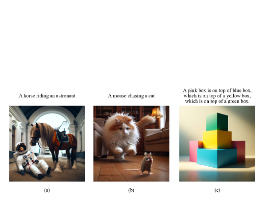
Figure 1: Example images generated by DALL·E3. In all three cases, entities and relations are common but their compositions are uncommon. DALL·E3 tends to (a) compose entities unnaturally, (b) get trapped by the canonical relation, or (c) disregard the requested ordering. These errors are recurring across multiple trials, suggesting that DALL·E3 does not grasp the abstract notion of relations.

1 Introduction

A visual scene is compositional in nature [51]. Atomic concepts, such as entity and texture, are composed via relations [18]. Relations represent abstract functions that are not visually presented, but modulate the visual realization of concepts. For example, consider a scene “a cat is chasing a mouse”. It consists of atomic concepts: cat and mouse. “Chasing” defines a relation that is visually realized as certain postures and orientations of the cat and the mouse. Relations take concepts to fill their roles as functions take variables to fill their arguments. This process is known as role-filler binding [41, 12, 14, 2], where fillers are concrete values and roles are abstract positions.

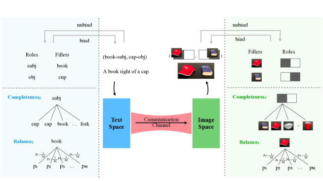
Figure 2: Conceptual Framework. Text-to-Image generation consists of three important distinct components: A text encoder, a visual decoder, and a mechanism to communicate between these two spaces. Generation of images with consistent spatial relations requires that 1) the text encoder distinctly encodes linguistic roles, 2) the image generator has the capacity to distinguish spatial roles in the output space, and 3) learning the correct mapping to translate linguistic roles to visual roles. Suppose the first two requirements are satisfied by pre-training or architectural expressivity, the remaining core task is to learn an effective communication channel, which is often instantiated as cross-attention layers in diffusion models. To this end, we propose statistical metrics to formally quantify how the training data distribution received by the communication channel affects generalization.

Due to abstractness, relations are always bound to concrete concepts in the space of observations, posting the challenge of truly grasping the abstract function of a relation and using it in generalizable ways, i.e. composing familiar relations with novel concepts. Recently pre-trained text-to-image models [3, 4, 40] unleash the power of image synthesis with unprecedented fidelity and controllability. However, as shown by Figure 1, a pre-trained model cannot generate images faithful to the relational constraints upon seeing uncommon entity-relation compositions. This implies that, pre-trained text-to-image models do not represent role-filler bindings independently of the fillers, leading to an important question of what hinders the learning of generalizable relations.

This work investigates this question from the data distribution angle. We conjecture that although pre-training ensures massive data quantity, it does not accomplish a proportionally large coverage of unique phenomena. Figure 2 shows our conceptual framework for text-to-image generation, consisting of three distinct components: A text encoder, a visual decoder and a mechanism to communicate between these two spaces. We formalize the underlying structure of the data as role-filler bindings which nicely capture the compositional connections between data points. We assume that architectural expressivity and pretraining already enable both the text encoder and the visual decoder to distinctly represent fillers and roles in their corresponding spaces. Based on this assumption, the communication channel becomes the key to task success. We believe the choice of supervision data crucially affects the behavior of the communication channel.

To this end, we introduce two metrics that quantify the skew of the underlying structure supported by a dataset. These two metrics take into account linguistic notion of roles and visual notion of roles respectively. Our hypothesis is that generalization failure of text-to-image model is a direct result of phenomenological incompleteness or imbalance under our metric. Our experiments in both synthetic images and natural images demonstrate the strong predictive power of our metrics on generalization performance.

2 Related Work

Text Conditioned Image synthesis Diffusion models initiate the tide of synthesizing photorealistic images in the wild. They benefit from training stability and do not exhibit mode collapse that GAN models suffer from. [50] feeds text prompts to the diffusion model to make the generation process controllable. Inspired by ControlNet, a myriad of works [28, 42, 47, 21, 40, 35] explore the integration of text encoders and image generators, such that image synthesis, editing and style-translation can be customized by users via text. Unlike diffusion models, Transformer-based image synthesis models are naturally better at working in coordination with text, due to the shared tokenization process [4, 23]. Transformer-based approaches perform on par with diffusion on fidelity, and are believed to have greater potential for resolving long-range dependency and relational reasoning [30], thanks to their patch-based representations and attention blocks. However, Transformers suffer from a discrete latent space and slow inference speed. The latest work [30] integrates a Transformer architecture and diffusion objectives, aiming at the best of both worlds.

Despite high fidelity scores, a recurring problem is the difficulty to generate objects in unfamiliar relations [25] Although those unfamiliar relations rarely occur in a natural collection of images, they are not physically implausible, and humans have no trouble producing a corresponding scene. This has drawn attention to evaluating generative models and characterizing such failures. Works along this vein suggest that generative models typically fail at multiple objects, with multiple attributes or relations [8, 13], where generalization to novel combinations of familiar components is needed the most.

Compositional generalization in image synthesis Compositional generalization is a specific form of generalization where individually known components are utilized to generate novel combinations. This remarkable learning ability has been widely studied in the vision-and-language understanding domain [39, 22, 32, 19, 38, 44, 15]. The text-to-image literature has recently seen efforts towards constructing images compositionally [49, 45, 7]. Closest to ours are two previous works that characterize properties of the underlying phenomenon space not trivially revealed by the pixel space. [29] has investigated shape, color and size as domains of atomic components, which can be combined to form tuples, e.g. (big, red, triangle). They mainly argue that generalization occurs under two conditions: 1) small structural distance between training and testing instances, and 2) effectively learning the disentanglement of attributes (i.e. a change in the size input will not affect the color output). [43] first assumes compositional data are formed by combining individually complex components with simple aggregation functions. Then they defined compositional support and sufficient support over a set of components, which are sufficient conditions for a learning system that compositionally generalizes.

Motivated by failures existing methods, we investigate data-related factors that affect the generalization performance. There is a possibility that better architectural design can complement high-quality data to achieve generalization.

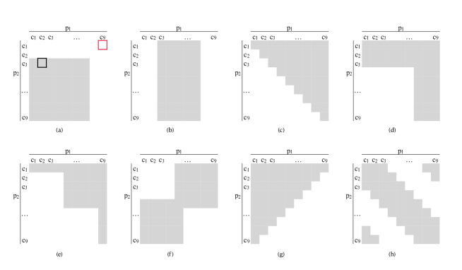
Figure 3: Sketched illustrations of phenomenological coverage with different properties. Shaded areas represent the training set, while blank areas represent the testing set. Columns and rows are organized by the concepts bound to position 1 and position 2 respectively. For example, the black cell in (a) represents the training instance ($c_{2}/p_{1},c_{3}/p_{2}$), the red cell in (a) represents the testing instance ($c_{9}/p_{1},c_{1}/p_{2}$). (a) Both positions are incomplete (b) Only $p_{1}$ is incomplete (c) Complete but unbalanced (d) Complete but unbalanced (e) Complete but unbalanced (f) Complete and balanced (g) Complete and balanced (h) Complete and balanced

3 Formalization

We start by formalizing scene construction as role-filler bindings. A scene is constructed by binding fillers denoted as $\mathbf{F}=(f_{1},\ldots,f_{K})$ to roles denoted as $\mathbf{R}=(r_{1},\ldots,r_{K})$. Roles and fillers are paired up by their indices. Hence, each scene representation involves the same number of roles and fillers, i.e., $|\mathbf{F}|=|\mathbf{R}|=K$. Using $\psi$ to denote the binding operation, a scene can be formalized into: $\psi(\mathbf{F},\mathbf{R})=(f_{1}/r_{1},...,f_{K}/r_{K})$ and we call $(f_{k},r_{k})$ a role-filler pair.

We would unbind a filler from $\psi(\mathbf{F},\mathbf{R})$ via the unbinding operation $\psi^{-1}$: $\psi^{-1}\Big{(}\psi(\mathbf{F},\mathbf{R}),f_{k}\Big{)}=r_{k}$. The unbinding operation describes the process of extracting the role from a binding that a given filler has been bound to, which corresponds to the decomposition of a compositional structure. Assume that $\psi^{-1}$ returns $null$ if the input filler $f_{k}$ does not exist in the scene.

Fillers are atomic concepts that can be selected from a set of concepts $\mathcal{C}=\{c_{1},...,c_{N}\}$ while roles can take values from a set of candidate positions $\mathcal{P}=\{p_{1},\ldots,p_{M}\}$. Typically, roles can have intrinsic meanings independent of the meanings of fillers [41]. For instance, the meaning of “upper position" is determined by the y-axis in a 2D image coordinate system, which exists independently of the specific pixel values that fulfill this role in each image. The meanings of roles can be either learned from the task structure or manually designed. In the text-to-image case, the task structure naturally invites two ways to define roles, corresponding to the linguistic and the visual space, respectively. From the linguistic perspective, we consider grammatical positions, e.g. $\mathcal{P}_{L}=\{subject,object\}$. From the visual perspective, we consider spatial positions, e.g. $\mathcal{P}_{V}=\{top,bottom\}$.

Under our definitions, each image is a scene. Therefore, an image dataset can be essentially abstracted as a collection of bindings: $\mathcal{D}=\{\psi(\mathbf{F}^{i},\mathbf{R}^{i})\}_{i=1,...,|\mathcal{D}|}$, where $\mathbf{F}^{i}$ and $\mathbf{R}^{i}$ denotes the fillers and roles in the $i$-th image. Let $\mathcal{U}=\mathcal{C}\times\mathcal{P}$ be the universe of all possible bindings. The vanilla notion of coverage supported by a dataset is the proportion of $\mathcal{U}$ that has non-zero supporting examples in the dataset: $\textbf{Coverage}(\mathcal{D})={|Deduplicate(\mathcal{D})|}/{|\mathcal{U}|}$, where the $Deduplicate$ removes examples with equivalent role-filler representations. We argue that this metric overlooks how elements in $\mathcal{U}$ are structurally connected. For instance, each element in $\mathcal{U}$ shares a common role or filler with other elements. Without taking this structural property into account, truly meaningful coverage of diverse and unique phenomena might be conflated by the seemingly diverse surface forms.

Motivated by this consideration, our proposed metrics aim to measure whether a dataset has support for every concept occurring in every position, as well as the probability distribution of the positions that each concept has been bound to. Next, we formally describe completeness and balance metrics by conveniently leveraging the notations of binding and unbinding operators.

3.1 Completeness

Completeness requires that every relation has been bound with every concept across the entire dataset. In this sense, we define:

$$\textbf{Completeness}(p_{m},\mathcal{D})=\frac{\Big{|}\Big{\{}c_{n}~{}\Big{|}p_{m}\in\psi^{-1}(\mathcal{D},c_{n}),c_{n}\in\mathcal{C}\Big{\}}\Big{|}}{|\mathcal{C}|},$$ (1)

where the operator extracting a concept from a dataset is defined as:

$$\psi^{-1}(\mathcal{D},c_{n})=\bigcup_{i=1}^{|\mathcal{D}|}\Big{\{}\psi^{-1}\left(\psi(\mathbf{F}^{i},\mathbf{R}^{i}),c_{n}\right)\Big{\}}.$$ (2)

Note that a fully complete dataset has completeness scores of 1 for all relations. Then we aggregate by taking the expected value to obtain the completeness over the entire dataset:

$$\begin{split}\textbf{Completeness}(\mathcal{D})&=\operatorname*{\mathbb{E}}\Big{[}\textbf{Completeness}(p_{m},\mathcal{D})\Big{]}\\ &=\sum_{p_{m}\in\mathcal{P}}\mathbb{P}(p_{m})\textbf{Completenss}(p_{m},\mathcal{D}).\end{split}$$ (3)

3.2 Balance

Balance requires that every concept is bound with each position with equal probability. Concretely, we first calculate the entropy of all positions that a given concept $c_{n}$ was bound to within dataset $\mathcal{D}$:

$$\textbf{Balance}(c_{n},\mathcal{D})=Entropy\Big{[}\psi^{-1}\Big{(}\psi(\mathbf{F}^{i},\mathbf{R}^{i}),c_{n}\Big{)},{i=1,...,|\mathcal{D}|}\Big{]},$$ (4)

where the function $Entropy$ computes the entropy of the distribution of the positions. Note that we constrain the computation to practical positions, i.e., excluding $null$ during the calculation process. Then we aggregate by taking the expected value to obtain the balance over the entire dataset:

$$\textbf{Balance}(\mathcal{D})=\operatorname*{\mathbb{E}}\Big{[}\textbf{Balance}(c_{n},\mathcal{D})\Big{]}=\sum_{c_{n}\in\mathcal{C}}\mathbb{P}(c_{n})\textbf{Balance}(c_{n},\mathcal{D}).$$ (5)

This metric is upper bounded by $\log(M)$, corresponding to the entropy of a uniform distribution over $\mathcal{P}$. The lower the metric, the higher the skew of a dataset. We normalize by $\log(M)$ to obtain a value within $[0,1]$.

So far we have defined completeness and balance for arbitrary sets of fillers and roles. Hereinafter, we will focus on binary relations that control two role-filler pairs, i.e. $|\mathbf{F}|=|\mathbf{R}|=2$. We use subscripts _L and _V to denote the linguistic and visual perspectives under which a metric is computed. In practice, we estimate each metric with empirical counts. Next, we conduct experiments to demonstrate that generalization is hindered by incompleteness or imbalance under either perspective.

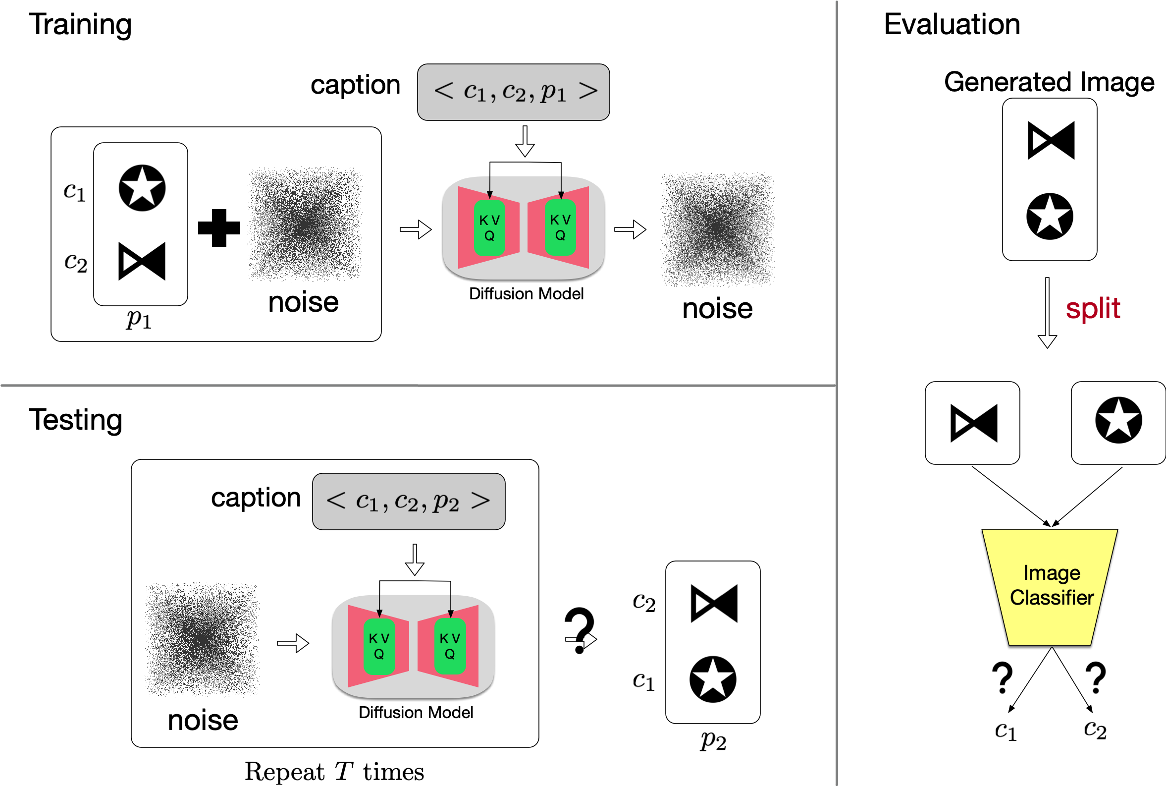
Figure 4: Training, testing and evaluation pipeline. We train diffusion models to generate images of two concepts ($c_{1}$, $c_{2}$) with a specified spatial relation. Then the model is tested on unseen concept pairs to see whether the learned relations are generalizable.

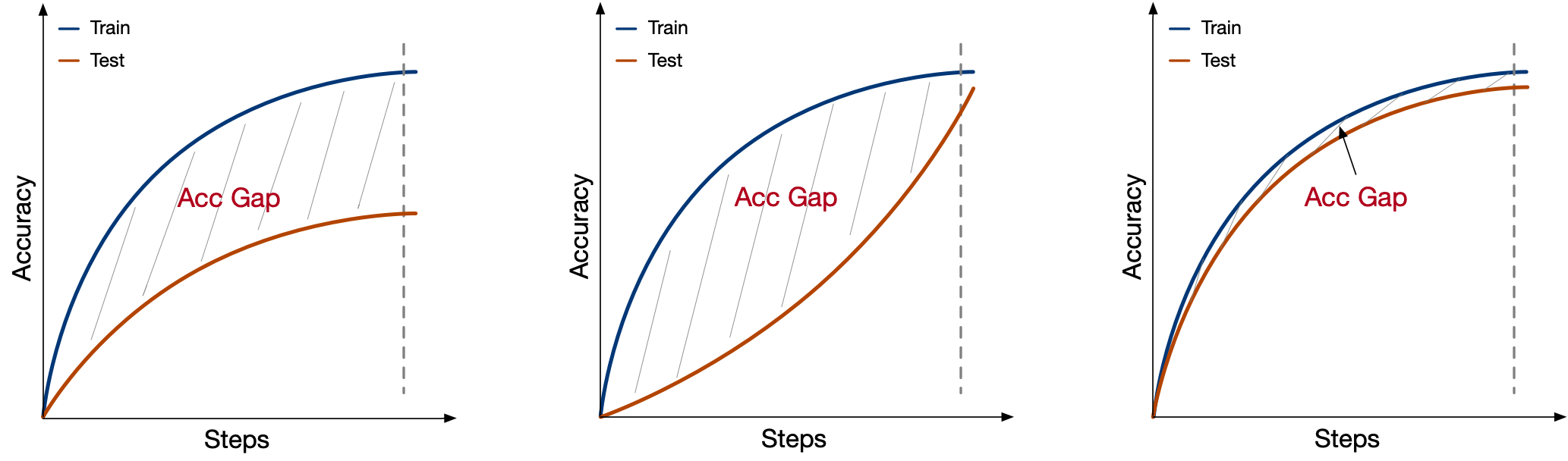
Figure 5: Three types of learning dynamics are observed in our experiments. In the worst scenario (left), the testing accuracy plateaus and never converges. In the best scenario (right), the testing accuracy closely tracks the training accuracy until both converge to perfect. In the middle scenario (center), the testing accuracy climbs slower than the training accuracy, but is still able to converge to perfect at a delayed point after the training accuracy has already converged. In order to distinguish between the middle and best scenarios, we report the accumulative gap between training and testing accuracy curves alongside the final testing accuracy. The accumulative gap captures the timeliness of generalization.

4 Experiments on Synthetic Images

4.1 Setup

We use a set of unicode icons as concepts, and assign common nouns to them as their names. We vary the number of concepts, $N$, within $\{30,40,50,60,70,80,90\}$. We consider two symmetric binary relations: "on top of", "at the bottom of". Images are constructed by drawing each icon on a 32x32 canvas, then stacking two icons vertically, resulting in 32x64 resolution. Captions are created from the template: "a(an) <icon_name> is <relation> a(an) <icon_name>".

Training sets ($\mathcal{D}$) are sampled from $\mathcal{U}$ with systematic control for the four properties: Completeness_L, Completeness_V, Balance_L, Balance_V. Importantly, to avoid confounders, we ensure the linguistic metrics are perfect when studying the effect of the visual metrics, and vice versa. Figure 3 illustrates training distribution with varied properties. We take the complementary set, $\mathcal{U}\setminus\mathcal{D}$ as the testing set. Note, all testing instances are unseen in terms of the tuple representation $(f_{1},r_{1},f_{2},r_{2})$. Yet we show that perfect generalization on the testing set is possible when the training set properly supports the phenomena space, i.e. being complete and balanced.

Our training, testing and evaluation pipeline is depicted in Figure 4. Following the architecture of [11], we train 350M UNet models on text-conditioned pixel-space diffusion, with T5-small [34] as the text encoder. The size of UNet is determined such that it is minimally above the threshold at which the model is capable of fully fitting the training set. This would avoid issues such as a lack of expressivity or under-training of an overparameterized model. For evaluation, we compute accuracy of both icons being generated correctly. The evaluation process is automated by pattern-matching icons with convolutional kernels.

Alongside the final testing accuracy, we report the accumulative difference between training and testing accuracy curves. This is because we have observed a third type of learning dynamics lying in between a generalization success and generalization failure, where the testing accuracy climbs slower than the training accuracy, but is still able to converge to perfect at a delayed point after the training accuracy has already converged. Only reporting on final testing accuracy would mask the qualitative difference that captures a notion of how timely generalization occurs. Figure 5 illustrates the three distinct learning dynamics.

4.2 Results

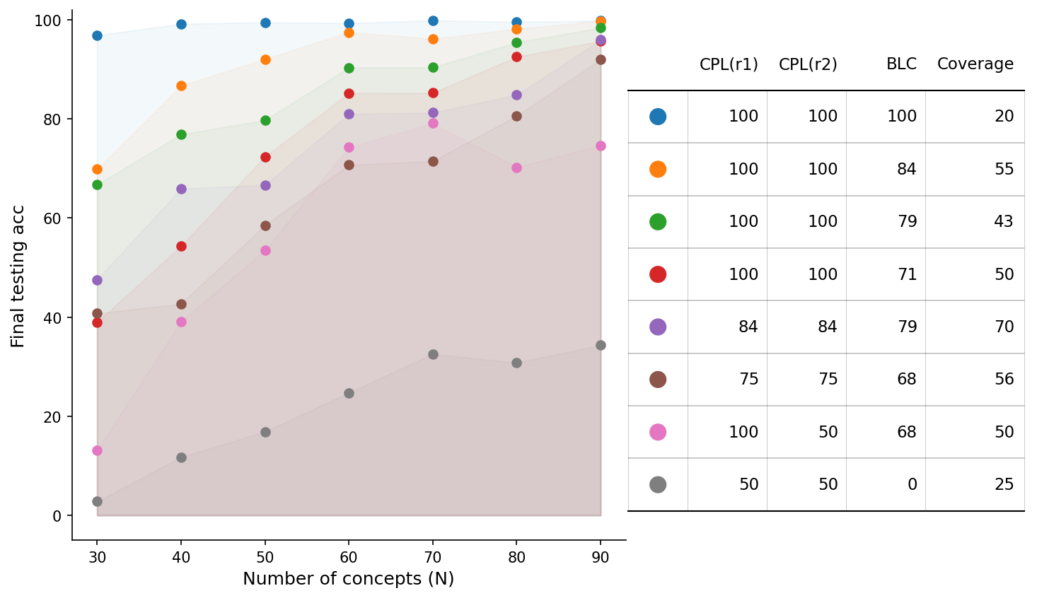
Figure 6: Under the definition of roles ($r_{1}$, $r_{2}$) from visual perspective (“top", “bottom"), the plot (left) shows final testing accuracy against distributional properties of the training set. The legend and the corresponding metrics are summarized in the table (right). The results suggest that both Completeness_V (CPL) and Balance_V (BLC) are positively correlated with testing (generalization) performance. By contrast, a vanilla notion of data coverage is badly correlated with performance.

Visual incompleteness significantly impedes generalization. The last four experiments in Figure 6 (indexed by purple, brown, pink and grey) have low Completeness_V. Their testing performance never reached 100%, even plateauing below 50% for smaller concept sets.

Visual imbalance harms generalization when $N$ is small. The first four experiments in Figure 6 (indexed by blue, orange, green and red) show the progression of increasing Balance_V while keeping full Completeness_V. As Balance_V grows, the testing accuracy consistently improves for all $N$. Increasing $N$ can provide a remedy for a dataset with complete but imbalanced support. In contrast, larger $N$ does not bring much help the support is incomplete.

Figure 7: Under the definition of roles ($r_{1}$, $r_{2}$), linguistically (“subj", “obj"), the plot shows final testing accuracy (left) and train-test accuracy gaps(right) against distributional properties of the training set. Legend and metrics are summarized in the table. The left plot suggests that linguistic incompleteness and imbalance harm generalization for small concept classes, while having less impact on the final testing accuracy for large concept classes. The right plot suggests that linguistic incompleteness and imbalance harm the timeliness of generalization, as indicated by larger train-test accuracy gaps.

Linguistic incompleteness or imbalance harms generalization to a lesser degree, but they delay generalization. Figure 7 (left) shows that all cases achieve perfect or near-perfect testing accuracy, unless for the very small concept classes. This suggests that linguistic incompleteness and imbalance do not severely hinder whether the model is able to generalize ultimately. However, they do bring a negative effect by delaying the onset of generalization. This delay effect is revealed in Figure 7 (right). The takeaway is that, although the final testing accuracy is comparable, lack of $\textbf{Completeness}_{L}$ or $\textbf{Balance}_{L}$ causes the testing acc to largely lag behind training acc, which takes a longer time to catch up. Similarly, we plot the generalization gap for the set of visual skew experiments in the appendix, observing the same trend. However, since both failing to generalize or having a prolonged duration before generalizing can lead to a large gap, this result has to be taken with a grain of salt.

Vanilla notions of coverage are a bad predictor for generalization. The rightmost columns in Figures 6 and 7 provide the training set’s coverage (%) over the universe $\mathcal{U}$. It can be seen that this does not correlate with the generalization performance. For example, the green run in Figure 6 outperformed red, purple, brown and pink runs, while having a much lower coverage than them. Also noteworthy is that we intentionally select low-coverage datasets to demonstrate the fully-complete, fully-balanced case, which achieves perfect generalization for all $N$. This strongly indicates the problem of aiming for a generalizable model by recklessly scaling up coverage. In accordance with research on model bias, we argue that scaling up along the incorrect axes is dangerous because it may aggravate unintended bias, without necessarily benefiting generalization.

Increasing $N$ eases generalization in all cases. The model consistently generalizes better when trained on more concepts, albeit to varying degrees. Figures 6 suggests that enlarging $N$ is more helpful when the data is within a decent range of Completeness_V and Balance_V (e.g. 70-80).

5 Experiments on Natural Images

5.1 Setup

We extend our experiments to natural images using the What’sUp benchmark proposed by [16]. Our hypothesis is that higher Completeness and Balance of the training distribution lead to more generalizable learning outcomes. Each image in the What’sUp benchmark contains two objects, with a caption describing their spatial relations. The spatial relations include two pairs of symmetric binary relations: left/right of and in-front/behind. Without loss of generality, we study left/right of, leaving the exploration of more than two relations for the future.

From an initial (complete and balanced) set of 308 samples with 15 unique concepts, subsamples are drawn where completeness and balance vary. For fair comparisons, the coverage of all subsamples is relatively the same. We train 470M pixel-space diffusion models on What’sUp image-caption pairs, with 64x32 resolution, 5e-4 learning rate and a batch size of 16. Early stopping is applied similarly to the synthetic setting. The length of training typically falls between 3000 and 6000 epochs. Hyperparameter tuning is described in the appendix.

Since under the natural image setting the same object may occur at different image positions, evaluation could not be performed with predetermined pattern-matching kernels. We finetune ViT-B/16 [6] as an automatic evaluation engine to classify the object in the left or right crop of generated images. A “blank” label is added to the classifier in order to indicate when a model fails to generate an object. Importantly, a secondary result of our work is demonstrating shortcomings of the widely used evaluation methods for image synthesis, such as CLIPScore [10], VQA with VLMs [26, 13], bounding-box evaluation with detectors [8, 13]. See Section 6 for discussions of when they fall short.

Table 1: What’sUp benchmark results varying Completeness_V and Balance_V

Training Set Properties				Performance
CPL($r_{1}$)	CPL($r_{2}$)	BLC	Cov.	Final Acc↑	Acc Gap ↓
100	50	63	47	18.75	84.55
80	73	77	50	19.52	73.87
87	87	75	49	25.93	68.41
100	100	73	44	10.17	80.49
100	100	88	49	28.50	64.89
100	100	100	48	48.64	33.67

Table 2: What’sUp benchmark results varying Completeness_L and Balance_L

Training Set Properties				Performance
CPL($r_{1}$)	CPL($r_{2}$)	BLC	Cov.	Final Acc↑	Acc Gap ↓
50	100	63	47	57.14	40.72
80	73	77	50	60.00	39.83
87	87	75	49	62.04	38.44
100	100	73	44	62.71	33.90
100	100	80	37	65.04	30.21
100	100	88	49	67.29	32.90

5.2 Results

On natural images, it is much harder to generalize, probably because the objects’ absolute position and postures can vary even when the relative spatial positions are determined. Another likely cause is the small number of concepts, as suggested by Section 4.2 that generalization tends to plateau at 50% for a small concept set. Nevertheless, the relative performance across different training set properties still conveys a meaningful message. Table 2 shows a consistent trend of generalization performance influenced by Completeness_V and Balance_V. The final accuracy gets higher and the generalization gap gets lower as the training distribution moves towards being fully complete and balanced. Completeness_L and Balance_L achieve a similar effect, as shown by Table 2.

As with our previous findings, visual skew imposes a more severe challenge, compared with the same amount of distributional skew on the linguistic side. Our explanation is that, since the network is modeling the pixel space, it is more directly affected by the skew of the observed pixel-space distribution, while skew of the language-space distribution impacts the result rather indirectly.

Upon closer examination of model outputs, the most common error was generating the correct objects with flipped order, suggesting that mapping fillers across domains is easy. However, learning to map roles from observations of role-filler binds is unsolved. Other errors include generating a blank or duplicating the object. Unlike the flippedOrder error, blank and duplication also occasionally occur when performing inference on the training set, likely as a result of undertraining. Figure 8 visualizes examples of correct and incorrect generations.

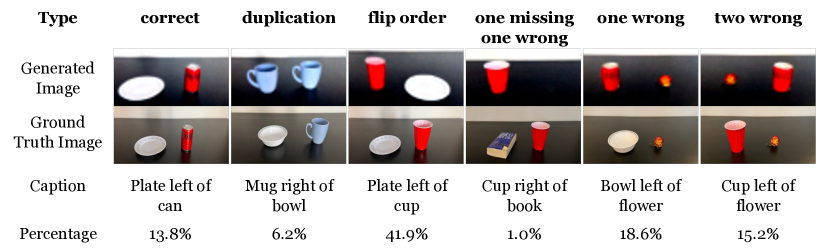
Figure 8: Qualitative examples of generated images and the corresponding ground truth images, including common failure types and their frequencies.

6 Discussions

We present a conceptual framework and formal metrics to study the contributing factors of generating images with correct spatial relations. Clearly, our work triggers many open questions and limitations that are worth future exploration.

Are Spatial Relations Distinguishable within the Text or the Image Domain Itself? We have mainly focused on what enables entity-relation compositions to be successfully conveyed from the text to the image domain. However, this question is meaningful only under the assumption that different roles and fillers are distinctly encoded in unimodal spaces. We have evidence that, perhaps surprisingly, this assumption does not always hold in existing approaches.

We train probing classifiers to extract the positional role of nouns from text encodings. More details are available in the appendix. We find that probes trained with the CLIP text encoder can only overfit the training data, but not generalizing. This indicates the inherent inability of CLIP text encoder to provide consistent signals of spatial positions This finding aligns with existing criticism on CLIP essentially being a bag-of-word model [48]. By contrast, probing experiments with T5 [34] encoder and the encoder of a pretrained vision-language model [9] succeed with near-perfect generalization. This makes T5 and VLMs naturally better candidates for training text-to-image models, and points out the inherent deficiency of CLIP for text-to-image.

On the image side, the capacity to represent positions can be theoretically guaranteed by image-patch positional encodings, readily compatible with attention blocks in the diffusion architecture. However, to our surprise, most of the open-source diffusion implementations [31] omit this step. We noticed this issue as our initial experiments failed unexpectedly. The problem was fixed after we modified the architecture to include image positional encodings. We posit that without positional encodings, there is almost no way to separate image patches based on their positions. Without this representational capacity, a model may heavily rely on pixel correlations and generalize in unexpected ways.

In short, we point out the importance of a text encoder that distinguishes positional roles and an image decoder that has the representational power for spatial information. We emphasize that these are not only an important precondition for our main analysis presented in this paper, but should also be a crucial consideration in future generative models or models that do spatial reasoning.

Text-to-Image Evaluation Methods We rely on several heuristics when automating the evaluation of generated images. This was feasible only when 1) objects are center aligned, and 2) the background is clean. Ultimately, we are interested in evaluating relations with cluttered scenes and with greater appearance variability. Besides finetuning a ViT classifier, we have attempted at existing off-the-shelf models, but found all of them are limited in one way or another. CLIPScore is known to have a tendency to ignore token orders. Indeed, CLIPScore judges correctly in only 37% of the times in our setting.

Evaluating spatial relations by comparing bounding box locations produced by detectors offers a more structured approach, yet it is restricted to the object classes available in the detection pretraining. For example, “headphones" and “tape" are classes in the What’sUp benchmark that do not belong to any of the popular detection datasets, rendering most of the detection models inappropriate for our experiments. Using open-vocabulary detectors [27] circumvents the problem with finite vocabularies. However, we find the following practical issues with open-vocabulary detectors, such as redundancy in the predicted bounding boxes and sensitivity to text prompts.

Aside from using CLIP and object detection, the literature has also suggested using vision-language foundation models (VLMs) for synthesized images evaluation. In addition to the apparent drawback of slow inference, it still remains questionable whether VLMs comprehend relations in the first place [48]. Our initial attempts to leverage LLaVA-VQA or BLIP2-VQA for auto-evaluation were unsuccessful for multiple reasons such as inability to recognize the relation , sensitivity to the question format, and unbalanced precisions across object classes. Please see the appendix for more results. We hope our experiments call into question the effectiveness of existing metrics on spatial consistency, which might have inadvertently masked the weakness of text-to-image models.

Generation in the Latent Space There are abundant studies on latent generation methods [36, 37, 4, 30] that are able to achieve higher resolution. However, the community has missed out on ensuring that the coverage of underlying phenomena has been proportionally scaled up with resolution. We believe increasing the phenomenological coverage and increasing resolution are both important, and argue that the progress towards spatially consistent high-resolution synthesis might be hampered by a lack of data support for structural phenomena. This work takes an initial attempt to formally measure phenomenological coverage and its amount of skew. We only studied pixel-space diffusion where the pixel-space coverage directly influences the structure of the model’s output space. We have also kept the image resolution small, to ensure the model capacity to fully fit the training data, thus avoiding confounding problems of undertraining. There are reasons to believe our conceptual framework can be extended to generation in the latent space. Firstly, the latent space feature maps have spatial correspondence with the image. Secondly, the VAE [17] does not have a language component, meaning that the entire language-to-vision communication channel still has to happen in the diffusion model. Though the VAE might have a structure that facilitates feature representation, it has not yet received any supervision for establishing the correspondence across modalities. To conclude, we leave the questions open on extending our formal notions to high-resolution images, latent generation methods as well as more nuanced relations.

7 Conclusion

Text-to-Image synthesis, despite recent breakthroughs in fidelity, appearance diversity and texture granularity, still struggles with relations. As the community strives for larger datasets to better cover the natural distribution, there is a lack of study on the axes along which phenomenological coverage can be meaningfully enlarged. This work presents the first effort to formally characterize training coverage, in the context of learning spatial relations. We introduce completeness and balance metrics under both the linguistic and visual perspectives. Our experiments on synthetic and natural data consistently suggest that models trained on more complete and balanced datasets have greater generalization potential. We see this work as a stepping stone towards text-to-image models that can faithfully generate relations in general, including implicit relations entailed by verbs. We hope to inspire research on structured image evaluation, architectures for modeling role-filler bindings and formal frameworks of generalization.

Appendix

Appendix 0.A Completeness and Balance Scores of Data in the Wild

Table A1: We parse three large-scale image-caption datasets, namely VGR, Nocaps, and Flickr30K. Then we compute Completeness and Balance on each corresponding subset involving spatial relations. LR stands for left-right, TB stands for top-bottom, and FB stands for front-behind. “-complete" means a subsample that is both linguistically and visually complete according to our definitions.

		Basic Statistics				Skew Metrics
	Dataset	#pairs	#unique images	#unique captions	#unique concepts	CPLV	CPLL	BLCV	BLCL
VGR	Original	21,944	—	—	—	—	—	—	—
	Spatial	19,419	4,348	12,163	885	—	—	—	—
	LR	15,482	3,244	9,816	695	80	100	93	99
	TB	2,505	1,553	1,513	439	66	73	49	62
	FB	11,162	527	834	209	69	95	58	98
	LR-complete	14,352	3,074	8,766	414	100	100	96	99
	TB-complete	784	488	395	77	100	100	57	69
	FB-complete	741	335	449	61	100	100	68	100
Nocaps	Original	45,000	—	—	—	—	—	—	—
	Spatial	14,583	3,827	14,241	2,975	—	—	—	—
	TB	12,726	3,540	12,714	2,273	63	62	35	31
	FB	1,854	1,051	1,854	703	65	64	57	45
	TB-complete	4,922	2,176	4,921	369	100	100	46	48
	FB-complete	718	491	718	110	100	100	75	62
Flickr30k	Original	155,070	—	—	—	—	—	—	—
	Spatial	44,918	20,784	43,419	4,205	—	—	—	—
	TB	37,541	18,436	37,462	3,003	67	66	36	29
	FB	7,351	5,333	7,350	1,483	65	63	57	38
	TB-complete	30,162	16,132	30,102	872	100	100	38	31
	FB-complete	4,016	3,185	4,016	265	100	100	66	48

On a high level, we seek to identify the causes for the dissatisfying relation learning in text-to-image generation from the data distribution angle. Our theory shows promising predictivity both on synthetic images and on real images captured in a clean and controlled setting. Ultimately, we expect to extend our investigation to real images in the wild. To facilitate research along this vein, we have parsed and analyzed three large-scale image-caption datasets, namely VGR (Visual Genome Relation) [48], Nocaps (Novel Object Captioning) [1], and Flickr30K [46]. We draw subsamples by matching spatial phrases in the captions for three spatial relations: left-right (LR), top-bottom (TB) and front-behind (FB). We present Completeness and Balance scores, along with basic statistics for each of these subsamples in Table A1.

VGR is carefully curated from Visual Genome [18] for the study of relational understanding in vision-language models. Thus, most of the examples in VGR involve a spatial relation. On the other hand, only a small subset in Nocaps or Flick30k contains spatial information. The supportive data size further shrinks if we constrain our subsamples to be complete under our definition. As can be seen from highlighted rows in Table A1, the largest complete subsample only constitutes a tiny fraction of the original data, plus being highly unbalanced. This emphasizes the importance of designing architectures or algorithms to enable generalization even from skewed data sources.

Appendix 0.B Experiments on Synthetic Data — Additional Results

Figure A1 plots for the train-test accuracy gap under varying Completeness_V and Balance_V scores. Moreover, detailed learning curves are comprehensively presented in Figure A2 and A3.

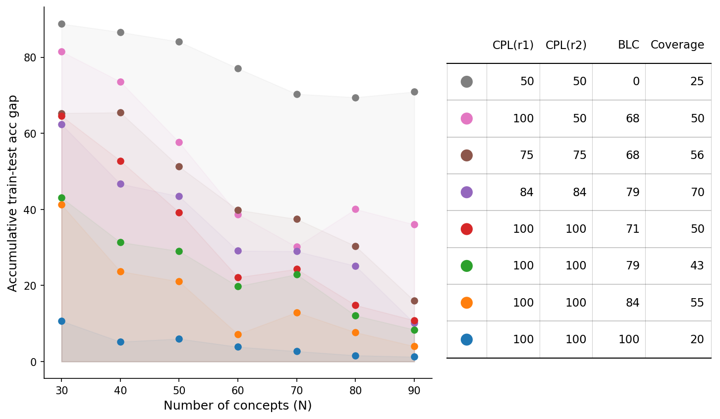
Figure A1: Under the definition of roles ($r_{1}$, $r_{2}$) from visual perspective (“top", “bottom"), the plot shows final testing accuracy against distributional properties of the training set. Legend and corresponding metrics are summarized in the table. This plot suggests that visual incompleteness and imbalance lead to larger gaps because both the final generalization performance and generalization speed are hampered.

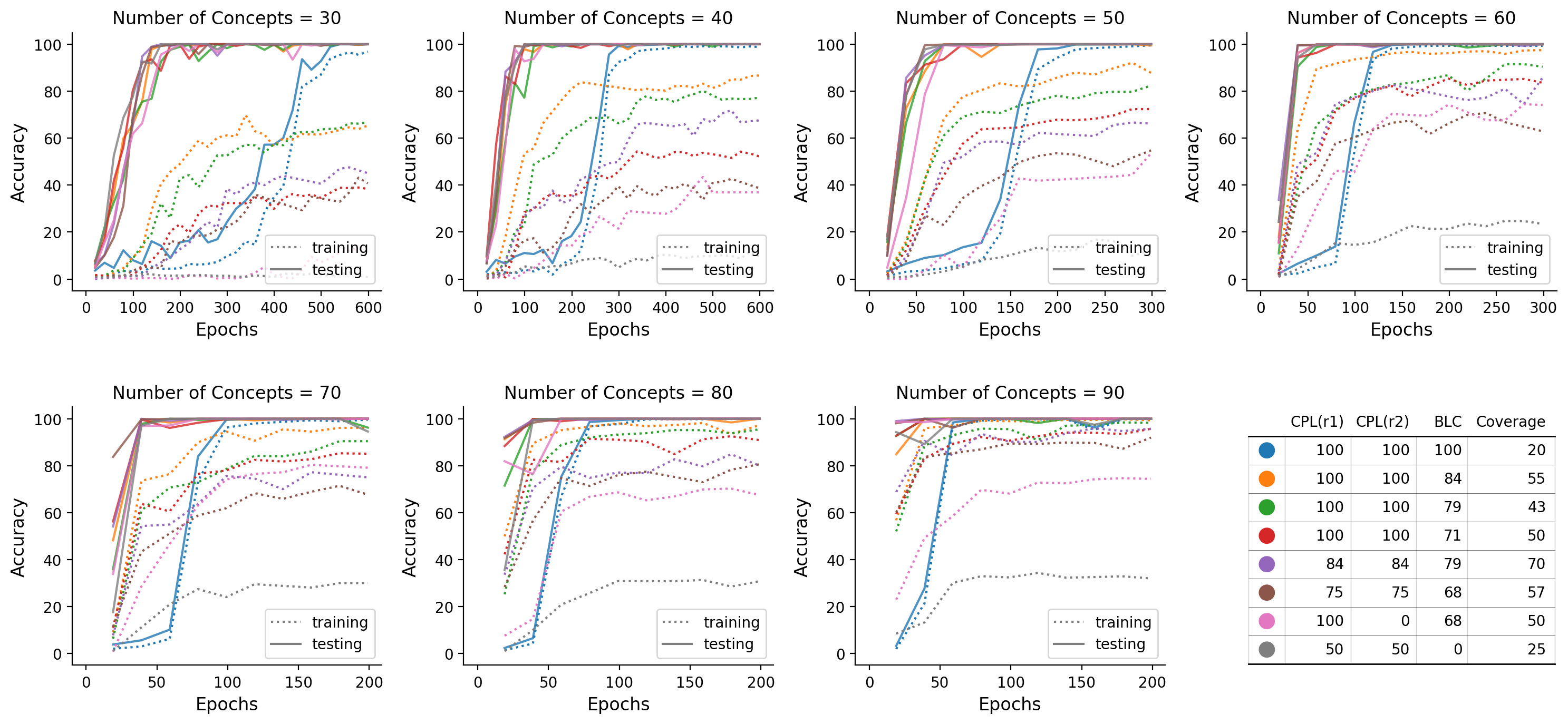
Figure A2: Detailed results on the impacts of Completeness_V and Balance_V. Panels are separated according to the number of concepts. Training accuracy always converges to perfect, whereas testing accuracy is hampered to varying degrees by visual incompleteness or imbalance. This degradation is more severe for a small number of concepts.

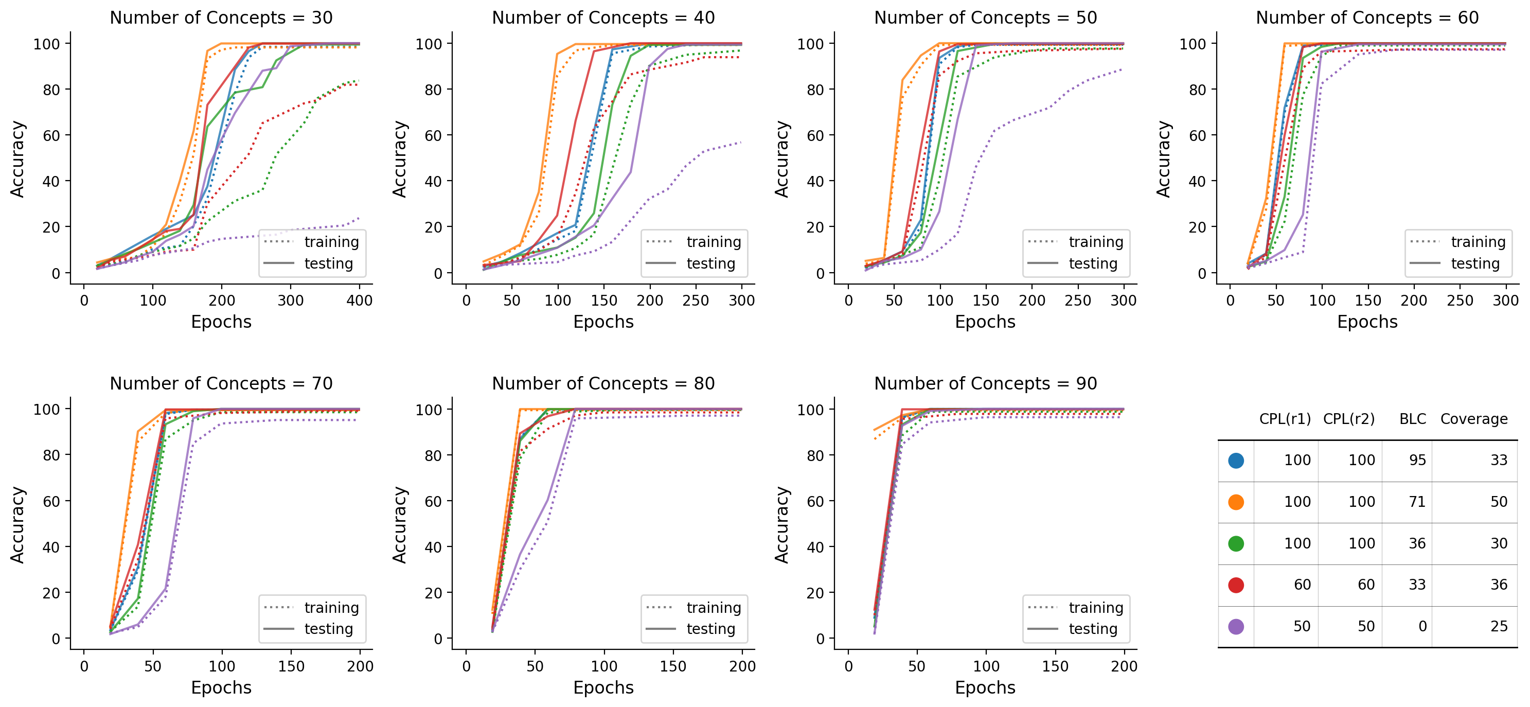
Figure A3: Detailed results on the impacts of Completeness_L and Balance_L. Panels are separated according to the number of concepts. Training accuracy always converges to perfect, whereas testing accuracy is hampered to varying degrees by linguistic incompleteness or imbalance. This degradation is more severe for a small number of concepts.

Appendix 0.C Probing Experiments on Text Encodings

Table A2: Probing results, showing that CLIP text encodings do not effectively facilitate subsequent modules to figure out the spatial positions of physical entities. In contrast, T5 and VLC are better candidates for coupling with text-to-image models.

Configuration		Performance
Text Encoder	MLP Num_layers	Tr Acc	Val Acc	Out-distr. Te Acc
CLIP-B/32	1	74.8	74.8	74.4
CLIP-B/32	2	74.6	74.4	74.2
CLIP-B/32	3	74.9	73.9	74.3
CLIP-L/14	1	74.6	73.5	74.3
CLIP-L/14	2	74.8	74.3	74.6
CLIP-L/14	3	75	74.9	74.5
T5-small	1	98.5	98.5	93.1
T5-small	2	100	100	95.8
T5-small	3	100	100	96.7
T5-flan-xxl	1	99.9	99.8	99.3
T5-flan-xxl	2	100	100	99.8
T5-flan-xxl	3	100	100	99.4
VLC-L/16	1	99.1	99.1	96.1
VLC-L/16	2	99.9	100	96.0
VLC-L/16	3	100	100	99.8

In the main paper, a conceptual framework for text-to-image generation is introduced, containing three components: text encoder, communication channel and image decoder. We have argued that the text-to-image generation performance crucially depends on all three components functioning and coordinating appropriately. Concretely, the text encoder is responsible for representing features extracted from raw text. The communication channel aims at transmitting features cross-modality. Lastly, the image decoder instantiates an output into the pixel space. Note, though we conceptually divide up the pipeline into three components, there is no hard boundary for the points at which different functions actually take place, because all representations and transformations in this pipeline are homogeneously encoded as differentiable parameters. For example, a weak text encoder could under-process the text features, thus expecting the communication channel to further process text features on the fly. In other words, while it is convenient to consider three types of responsibilities for developing hypotheses regarding the sources of error, under the hood, those three components in an end-to-end system could easily transfer or take over responsibilities to or from each other.

This raises the question: How rich text features from pre-trained text encoders are? Based on our argument above, richer text features would give the subsequent communication channel an advantage point, since it remains to perform relatively simple transformations to transmit the key message cross-modality. This intuition aligns with the known benefit of representation learning, as it saves efforts for modeling downstream tasks. On the other hand, a less capable text encoder would increase the difficulty of learning the communication channel, and even create obstacles if critical information gets lost.

To this end, we perform probing experiments to analyze how good an advantage point a text encoder can provide for learning a communication channel. We consider three pre-trained text encoders: CLIP [33], T5 [34] and VLC [9], which are chosen to be representative of different model families and pre-training objectives. CLIP is an encoder-only dual architecture pre-trained with image-text contrastive loss. T5 is an encoder-decoder architecture pre-trained with the causal language modeling loss. VLC is an encoder-only multimodal architecture pre-trained with masked language modeling, masked image modeling as well as image-text matching objectives. Pertaining to our work, the core responsibility of the communication channel is to translate linguistic fillers and roles to the corresponding visual entities and spatial positions. Thus, we train probing classifiers to label the noun tokens in a caption with spatial positions (e.g. top or bottom). For example, given a caption “a book is on top of a cup”, we apply an MLP on the encoded features of the “book” and “cup” tokens, and expect the MLP to output label 0 for “book” and label 1 for “cup”. For another example, “a laptop is at the bottom of a phone”, the MLP should output label 1 for “laptop” and label 0 for “phone”. The probing performance signifies the utility of a pre-trained text encoder in assisting a diffusion model, particularly in the context of generating spatial relations. Though a probing classifier is a drastic simplification, we believe that it still captures the main problem.

We select 200 common English nouns meaning concrete objects, then divide them into 170 “in-distribution” and 30 “out-of-distribution” nouns. We expect a successful probe to generalize to out-of-distribution nouns, which would strongly imply the existence of robust feature directions encoding spatial information. We train 1-, 2-, and 3-layer MLPs with ReLU nonlinearities. The 1-layer MLP is equivalent to linear probing. The MLPs are trained for 10-20 epochs until convergence. We observe consistent results across random data-splitting outcomes (5 seeds) and hyperparameters such as learning rate ({1e-3, 1e-4}) and batch size ({16, 64}). Table A2 summarizes our results. CLIP struggles to exceed 75% and this cannot be improved by increasing the encoder size or the number of MLP layers. T5-small achieves perfect in-distribution performance, but makes minor mistakes when generalizing out-of-distribution. T5-flan-xxl [5] achieves perfect accuracy in all three splits. VLC performs on par with T5-flan-xxl in-distribution, and slightly underperforms T5-flan-xxl out-of-distribution.

Our experiments in this section undermine CLIP-text-encoder’s effectiveness in facilitating subsequent modules to figure out the spatial positions of physical entities. In contrast, T5 and VLC are better candidates for coupling with text-to-image models. Indeed, our ablation study on diffusion models confirms this claim. As shown in Figure A4, all experiments follow the same setting except that solid lines represent the T5-small text encoder and dotted lines represent the CLIP-B/16 text encoder. It is evident that dotted lines consistently fall behind solid lines. Note, our analysis does not render CLIP as incapable of serving as the text encoder for text-to-image models. Nevertheless, compared to T5 and VLC, CLIP might have to offload more burden to the communication channel for nontrivial processing.

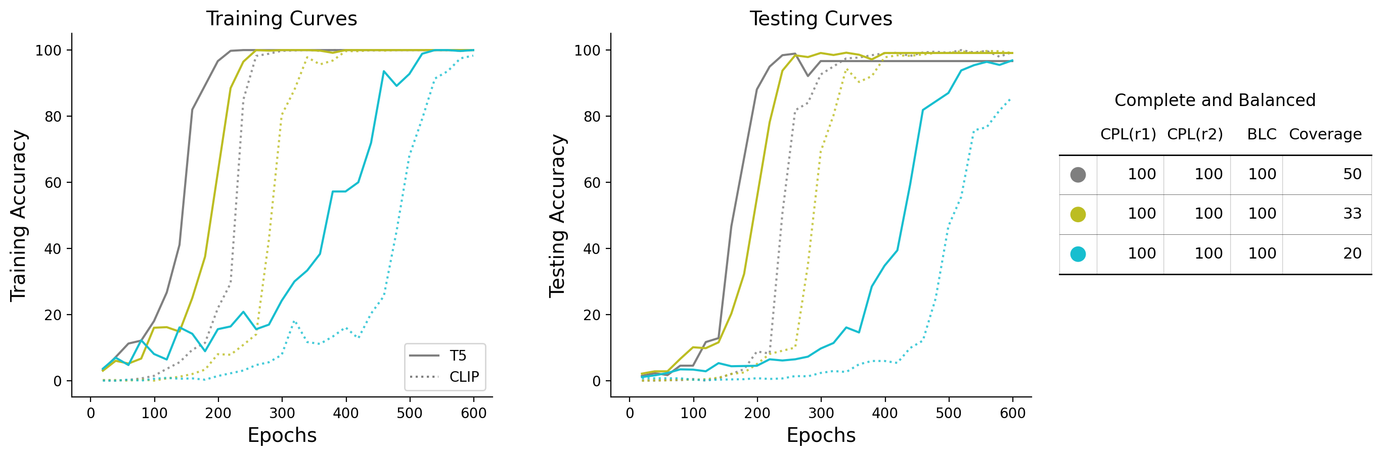
Figure A4: Ablation study on the text encoder while keeping all other training configurations fixed. The performance of diffusion paired with CLIP text encoder consistently falls behind the performance with T5, suggesting that CLIP would indeed make learning harder and slower.

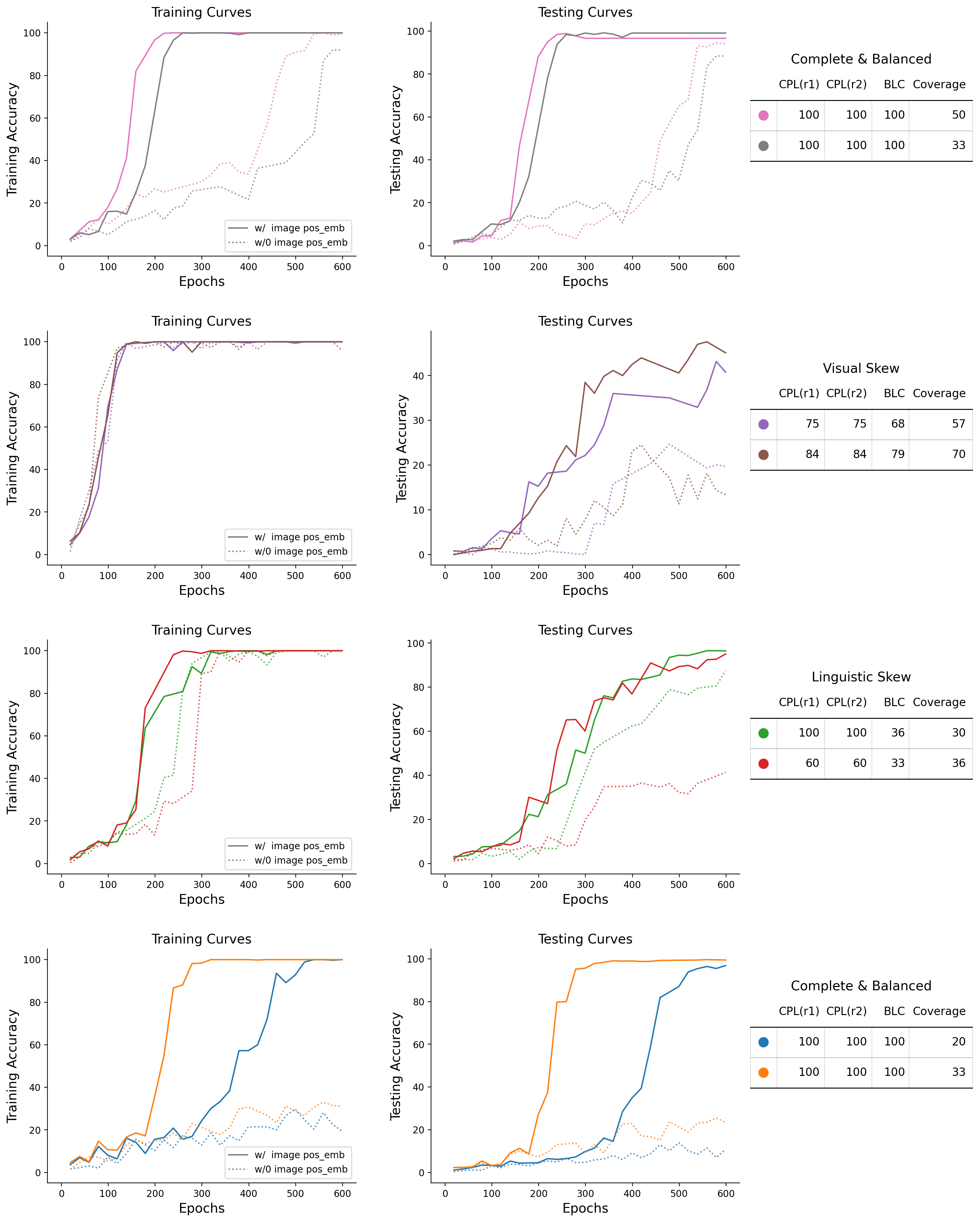
Figure A5: Ablation study on whether to include image positional embeddings. We see that diffusion models without the image positional embedding are inferior to their counterparts across all panels, albeit failing or underperforming for different reasons.

Appendix 0.D Ablation Results on Image Positional Embeddings

In this section, we investigate a crucial factor — image positional embeddings — that draws a connection from spatial features to the correct absolute positions in the 2D image coordinates. Without explicitly embedding patch positions, such ability could be largely damaged. Though, arguably, zero-paddings in the convolutional layers could provide complementary positional information, we believe that this cannot fully compensate for the loss incurred by a lack of explicit image positions. We perform ablation studies where the image positional embeddings are removed while remaining other architectural components intact. Specifically, we set the number of concepts to be 30 because a smaller number of concepts imposes a greater challenge such that discrepancies in performance can be easily revealed.

Figure A5 presents the results of this ablation study. For notational convenience, we call models with image positional embeddings the “Pos-models", and call models without image positional embeddings the “NoPos-models". It can be observed that, NoPos-models perform worse than their counterpart Pos-models across all panels. Comparing the panels between rows, we identify different types of failure. In the first row (pink and grey), NoPos-models exhibit much slower convergence speed, but are still able to converge and generalize eventually. In the second row (purple and brown), NoPos-models do not fall behind in terms of training accuracy. Yet they are generalizing to the testing set much worse than Pos-models. In the third row (green and red), there are small gaps between Pos-models and NoPos-models in training accuracy. And this gap widens regarding testing accuracy. In the fourth row (blue and orange), unfortunately, NoPos-models have trouble even fitting the training set.

We attempt to associate the failure patterns of NoPos-models with our proposed linguistic or visual skew in the training data. It appears that in rows 2&3, models are hampered by the skew, with NoPos-models being more severely hampered. When the training data is complete and balanced, the NoPos-models would generalize on larger coverages (row 1), albeit at much slower paces, and fail spectacularly on smaller coverages (row 4). We suspect that the interplay between the data skew and the failure pattern of NoPos-models is intricate, so we have not reached a conclusive statement. But the key takeaway is clear: removing image positional embeddings leads to notable performance degradation in all cases.

Appendix 0.E Auto-Evaluation of Relations — Failed Attempts and Discussions

Current evaluation methods of generated images have lingering issues of not paying attention to relations. However, our experiments critically depend on an auto-eval engine that correctly judges both the object identity and position. Off-the-shelf open-vocabulary detection models have problems such as insensitivity to certain tags, largely redundant predictions and poor reliability at low resolutions. Thus, we decide that they are not suitable for our purpose. We then try to leverage vision-language models, inspired by [13, 26], which ended up not working. Eventually, we arrive at a working solution via finetuning ViT [6], despite making certain compromises such as assuming that objects only occur at fixed image regions. This section describes our attempts with prompting VLMs and finetuning ViT for automatic evaluation.

0.E.1 Leveraging Large Vision-Language Models

Zero-Shot Multiple-Choice VQA

For evaluation, we initially attempted to use off-the-shelf Large Vision-Language Models (VLMs), including BLIP2 [20] and LLaVA1.5 [24], to directly extract positional relationships from the generated images, as their training sets include position extraction tasks, similar to those in Visual Genome [18]. The simplest approach to VQA is to pose a multiple-choice question. For example, the prompt could be “Which caption better describes the image? A. A mug to the right of a knife; B. A mug in

front of a knife; C. A mug behind a knife; D. A mug to the left of

a knife.” The zero-shot accuracy results are shown in Table A4. Both large vision-language models significantly underperform in handling positional relationships, with accuracy results just slightly better than the random baseline of 25%. Hence, we opted not to pursue further improvements on multiple-choice VQA tasks.

Table A3: Zero-Shot Multiple-Choice VQA Results of BLIP2 and LLaVA1.5 on the What’s Up Benchmark.

Model	Accuracy
BLIP2	0.26
LLaVA1.5	0.28

Table A4: Zero-Shot Object Detection Results of BLIP2 and LLaVA1.5 on the What’s Up Benchmark.

	BLIP2	LLaVA1.5
Acc. on True Labels	100%	83.6%
Acc. on False Labels	12.1%	94.2%
Average Accuracy	16.9%	93.6%

Zero-shot Object Detection

Though VLMs struggle to recognize positional relationships, we discovered that they excel in detecting the existence of objects. The process begins with cropping the image into a square, resizing it to 64x64 pixels, and then dividing it into two halves—either left/right or top/bottom, based on the true label. We then pose the question to each half: “Is a [object] in the image?”. The results, presented in Table A4, show that BLIP2 tends to affirm the presence of any queried object, leading to 100% accuracy for true labels but a significantly lower accuracy of 12.1% for false labels. Given that the dataset comprises 18 objects, questions with false labels outnumber those with true labels by 17 times, pulling the average accuracy close to that for false labels. LLaVA 1.5, however, shows a remarkable improvement, with an accuracy of 94.2% on false labels.

Table A5: LLaVA1.5 Zero-Shot Position Detection: accuracy improves after removing bad classes.

Improvement Strategy	Accuracy
Base Accuracy	0.68
Eliminate Bottom 2 Classes (Tape, Flower)	0.83
Eliminate Bottom 3 Classes (Tape, Flower, Knife)	0.87
Eliminate Bottom 4 Classes (Tape, Flower, Knife, Fork/Scissors)	0.89
Eliminate Bottom 5 Classes (Tape, Flower, Knife, Fork, Scissors)	0.92

Zero-shot Position Detection

Given LLaVA’s impressive performance in object detection, we explored using LLaVA for positional detection in a manual manner. The data processing procedure is the same as that in object detection. Subsequently, we ask, “Is a [object1] in image1?” and “Is a [object2] in image2?” A classification is deemed correct if both questions are affirmed. The initial accuracy stands at approximately 68.14%. To enhance this metric, we propose several strategies, including eliminating poorly performing classes as shown in Table A5. Removing the bottom two classes (tape and flower) elevates accuracy to about 83%, and eliminating the bottom three (tape, flower, and knife) boosts it to around 87%. Further exclusion of the bottom four classes, including fork or scissors, increases accuracy to 89%, and removing the bottom five classes (tape, flower, knife, fork, and scissors) results in an accuracy of 92%.

During the position detection experiments, we observed many mistakes, i.e., the model answers “yes” even when there is no such object in the image. We list the top 10 common failure cases in Table A6. Each pair contains the object that truly exists in the image and the mistaken one. Understandably, the model tends to confuse a mug for a cup and a can for a cap, as these nouns have similar semantic meanings.

Pair	Count
(Mug, Cup)	68
(Can, Cap)	36
(Bowl, Plate)	28
(Sunglasses, Headphones)	27
(Remote, Headphones)	27
(Scissors, Remote)	25
(Scissors, Headphones)	24
(Scissors, Cap)	21
(Flower, Candle)	21
(Candle, Cap)	19

Table A6: Top 10 common errors in Zero-Shot Position Detection with LLaVA1.5.

0.E.2 Crop and Classify

For the purpose of automatically evaluating the generated images on the What’sUp benchmark, we finally arrive at a working solution that consists of two steps. The first step obtains single object crops from an image based on heuristics such that the dividing line between two objects aligns with the center of the image. The second step classifies the object into one of the 15 classes. We obtain an Oracle classifier via finetuning ViT-B/16. We use individual object crops from the original images as our finetuning data, splitting into training and validation sets with the ratio 90:10. Examples are illustrated in Figure A6. We adopt the Adam optimizer with lr=2e-4 and a batch size of 16. The classification accuracy reaches perfect within 5 epochs. For sanity check, we manually examined 144 generated examples and our ViT evaluated correctly on all of them.

Figure A6: Finetuning data examples. We finetune ViT to classify objects in image crops for the purpose of automatically evaluating generated images.

Appendix 0.F Experiments on Synthetic Data — Details

0.F.1 Icons and Their Names

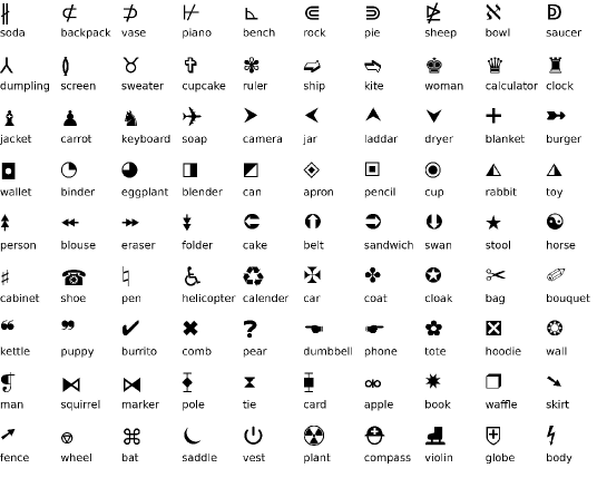
Figure A7: 90 icons paired with 90 common nouns as their names.

We consider unicode icons as concepts, each paired with a concrete noun as the identity. To create an image, we draw icons on a white canvas. Figure A7 shows 90 individual icons which we leverage in our synthetic experiments.

0.F.2 Model Configs

⬇

layers_per_block = 2

block_out_channels = (64, 256, 1024)

down_block_types = (

"DownBlock2D",

"CrossAttnDownBlock2D",

"CrossAttnDownBlock2D",

)

up_block_types = (

"CrossAttnUpBlock2D",

"CrossAttnUpBlock2D",

"UpBlock2D",

)

cross_attention_dim = 128

image_size = (64,32)

conv_in_kernel = 3

conv_out_kernel = 3

0.F.3 Training Configs

⬇

mixed_precision = "fp16"

noise_schedule = "squaredcos_cap_v2"

learning_rate = 1e-4

lr_warmup_steps = 1000

train_batch_size = 16

num_train_timesteps = 100 # diffusion steps

0.F.4 Hyperparameter Search

layers_per_block $\in$ {2, 3, 4}.
block_out_channels $\in$ {(32, 128, 512), (128, 256, 512), (64, 256, 1024), (64, 512, 2048)}.
learning_rate $\in$ {1e-3, 5e-4, 1e-4, 1e-5}.
train_batch_size $\in$ {8, 16, 64}.
lr_warmup_steps $\in$ {100, 1000, 2000, 5000}.

Appendix 0.G Experiments on Natural Data — Details

0.G.1 Model Configs

⬇

layers_per_block = 2

block_out_channels = (512, 512, 1024)

down_block_types = (

"DownBlock2D",

"CrossAttnDownBlock2D",

"CrossAttnDownBlock2D",

)

up_block_types = (

"CrossAttnUpBlock2D",

"CrossAttnUpBlock2D",

"UpBlock2D",

)

cross_attention_dim = 128

image_size = (32,64)

conv_in_kernel = 3

conv_out_kernel = 3

0.G.2 Training Configs

⬇

mixed_precision = "fp16"

noise_schedule = "squaredcos_cap_v2"

learning_rate = 5e-4

lr_warmup_steps = 1000

train_batch_size = 16

num_train_timesteps = 100 # diffusion steps

0.G.3 Hyperparameter Search

layers_per_block $\in$ {2, 3, 4}.
block_out_channels $\in$ {(64, 256, 1024), (128, 512, 1024), (512, 512, 1024), (512, 1024, 1536)}.
learning_rate $\in$ {1e-3, 5e-4, 1e-4}.
train_batch_size $\in$ {16, 64}.
lr_warmup_steps $\in$ {1000, 2000, 5000, 10000}.
num_train_timesteps $\in$ {100, 500, 1000}.

References

- [1] Agrawal, H., Desai, K., Wang, Y., Chen, X., Jain, R., Johnson, M., Batra, D., Parikh, D., Lee, S., Anderson, P.: Nocaps: Novel object captioning at scale. In: Proceedings of the IEEE/CVF international conference on computer vision. pp. 8948–8957 (2019)
- [2] Ajjanagadde, V., Shastri, L.: Rules and variables in neural nets. Neural Computation 3(1), 121–134 (1991)
- [3] Betker, J., Goh, G., Jing, L., Brooks, T., Wang, J., Li, L., Ouyang, L., Zhuang, J., Lee, J., Guo, Y., et al.: Improving image generation with better captions. Computer Science. https://cdn. openai. com/papers/dall-e-3. pdf 2(3), 8 (2023)
- [4] Chang, H., Zhang, H., Barber, J., Maschinot, A., Lezama, J., Jiang, L., Yang, M.H., Murphy, K., Freeman, W.T., Rubinstein, M., et al.: Muse: Text-to-image generation via masked generative transformers. arXiv preprint arXiv:2301.00704 (2023)
- [5] Chung, H.W., Hou, L., Longpre, S., Zoph, B., Tay, Y., Fedus, W., Li, Y., Wang, X., Dehghani, M., Brahma, S., et al.: Scaling instruction-finetuned language models. arXiv preprint arXiv:2210.11416 (2022)
- [6] Dosovitskiy, A., Beyer, L., Kolesnikov, A., Weissenborn, D., Zhai, X., Unterthiner, T., Dehghani, M., Minderer, M., Heigold, G., Gelly, S., et al.: An image is worth 16x16 words: Transformers for image recognition at scale. arXiv preprint arXiv:2010.11929 (2020)
- [7] Goel, V., Peruzzo, E., Jiang, Y., Xu, D., Sebe, N., Darrell, T., Wang, Z., Shi, H.: Pair-diffusion: Object-level image editing with structure-and-appearance paired diffusion models. arXiv preprint arXiv:2303.17546 (2023)
- [8] Gokhale, T., Palangi, H., Nushi, B., Vineet, V., Horvitz, E., Kamar, E., Baral, C., Yang, Y.: Benchmarking spatial relationships in text-to-image generation. arXiv preprint arXiv:2212.10015 (2022)
- [9] Gui, L., Chang, Y., Huang, Q., Som, S., Hauptmann, A.G., Gao, J., Bisk, Y.: Training vision-language transformers from captions. Transactions on Machine Learning Research (2023), https://openreview.net/forum?id=xLnbSpozWS
- [10] Hessel, J., Holtzman, A., Forbes, M., Bras, R.L., Choi, Y.: Clipscore: A reference-free evaluation metric for image captioning. arXiv preprint arXiv:2104.08718 (2021)
- [11] Ho, J., Jain, A., Abbeel, P.: Denoising diffusion probabilistic models. Advances in neural information processing systems 33, 6840–6851 (2020)
- [12] Holyoak, K.J.: Analogy and relational reasoning. The Oxford handbook of thinking and reasoning pp. 234–259 (2012)
- [13] Huang, K., Sun, K., Xie, E., Li, Z., Liu, X.: T2i-compbench: A comprehensive benchmark for open-world compositional text-to-image generation. Advances in Neural Information Processing Systems 36 (2024)
- [14] Hummel, J.E., Holyoak, K.J., Green, C.B., Doumas, L.A., Devnich, D., Kittur, A., Kalar, D.J.: A solution to the binding problem for compositional connectionism. In: AAAI Technical Report (3). pp. 31–34 (2004)
- [15] Johnson, J., Hariharan, B., Van Der Maaten, L., Fei-Fei, L., Lawrence Zitnick, C., Girshick, R.: Clevr: A diagnostic dataset for compositional language and elementary visual reasoning. In: Proceedings of the IEEE conference on computer vision and pattern recognition. pp. 2901–2910 (2017)
- [16] Kamath, A., Hessel, J., Chang, K.W.: What’s" up" with vision-language models? investigating their struggle with spatial reasoning. arXiv preprint arXiv:2310.19785 (2023)
- [17] Kingma, D.P., Welling, M.: Auto-encoding variational bayes. arXiv preprint arXiv:1312.6114 (2013)
- [18] Krishna, R., Zhu, Y., Groth, O., Johnson, J., Hata, K., Kravitz, J., Chen, S., Kalantidis, Y., Li, L.J., Shamma, D.A., et al.: Visual genome: Connecting language and vision using crowdsourced dense image annotations. International journal of computer vision 123, 32–73 (2017)
- [19] Lake, B., Baroni, M.: Generalization without systematicity: On the compositional skills of sequence-to-sequence recurrent networks. In: International conference on machine learning. pp. 2873–2882. PMLR (2018)
- [20] Li, J., Li, D., Savarese, S., Hoi, S.: Blip-2: Bootstrapping language-image pre-training with frozen image encoders and large language models. In: International conference on machine learning. pp. 19730–19742. PMLR (2023)
- [21] Li, Y., Liu, H., Wu, Q., Mu, F., Yang, J., Gao, J., Li, C., Lee, Y.J.: Gligen: Open-set grounded text-to-image generation. In: Proceedings of the IEEE/CVF Conference on Computer Vision and Pattern Recognition. pp. 22511–22521 (2023)
- [22] Lindemann, M., Koller, A., Titov, I.: Compositional generalisation with structured reordering and fertility layers. arXiv preprint arXiv:2210.03183 (2022)
- [23] Liu, H., Yan, W., Abbeel, P.: Language quantized autoencoders: Towards unsupervised text-image alignment. Advances in Neural Information Processing Systems 36 (2024)
- [24] Liu, H., Li, C., Li, Y., Lee, Y.J.: Improved baselines with visual instruction tuning. arXiv preprint arXiv:2310.03744 (2023)
- [25] Lovering, C., Pavlick, E.: Training priors predict text-to-image model performance. arXiv preprint arXiv:2306.01755 (2023)
- [26] Lu, Y., Yang, X., Li, X., Wang, X.E., Wang, W.Y.: Llmscore: Unveiling the power of large language models in text-to-image synthesis evaluation. Advances in Neural Information Processing Systems 36 (2024)
- [27] Minderer, M., Gritsenko, A., Stone, A., Neumann, M., Weissenborn, D., Dosovitskiy, A., Mahendran, A., Arnab, A., Dehghani, M., Shen, Z., et al.: Simple open-vocabulary object detection. In: European Conference on Computer Vision. pp. 728–755. Springer (2022)
- [28] Mo, S., Mu, F., Lin, K.H., Liu, Y., Guan, B., Li, Y., Zhou, B.: Freecontrol: Training-free spatial control of any text-to-image diffusion model with any condition. arXiv preprint arXiv:2312.07536 (2023)
- [29] Okawa, M., Lubana, E.S., Dick, R., Tanaka, H.: Compositional abilities emerge multiplicatively: Exploring diffusion models on a synthetic task. Advances in Neural Information Processing Systems 36 (2024)
- [30] Peebles, W., Xie, S.: Scalable diffusion models with transformers. In: Proceedings of the IEEE/CVF International Conference on Computer Vision. pp. 4195–4205 (2023)
- [31] von Platen, P., Patil, S., Lozhkov, A., Cuenca, P., Lambert, N., Rasul, K., Davaadorj, M., Wolf, T.: Diffusers: State-of-the-art diffusion models. https://github.com/huggingface/diffusers (2022)
- [32] Potts, C.: Compositionality or generalization? (2019)
- [33] Radford, A., Kim, J.W., Hallacy, C., Ramesh, A., Goh, G., Agarwal, S., Sastry, G., Askell, A., Mishkin, P., Clark, J., et al.: Learning transferable visual models from natural language supervision. In: International conference on machine learning. pp. 8748–8763. PMLR (2021)
- [34] Raffel, C., Shazeer, N., Roberts, A., Lee, K., Narang, S., Matena, M., Zhou, Y., Li, W., Liu, P.J.: Exploring the limits of transfer learning with a unified text-to-text transformer. The Journal of Machine Learning Research 21(1), 5485–5551 (2020)
- [35] Ramesh, A., Dhariwal, P., Nichol, A., Chu, C., Chen, M.: Hierarchical text-conditional image generation with clip latents. arXiv preprint arXiv:2204.06125 1(2), 3 (2022)
- [36] Rombach, R., Blattmann, A., Lorenz, D., Esser, P., Ommer, B.: High-resolution image synthesis with latent diffusion models. In: Proceedings of the IEEE/CVF conference on computer vision and pattern recognition. pp. 10684–10695 (2022)
- [37] Rombach, R., Blattmann, A., Lorenz, D., Esser, P., Ommer, B.: High-resolution image synthesis with latent diffusion models. In: Proceedings of the IEEE/CVF conference on computer vision and pattern recognition. pp. 10684–10695 (2022)
- [38] Ruis, L., Andreas, J., Baroni, M., Bouchacourt, D., Lake, B.M.: A benchmark for systematic generalization in grounded language understanding. Advances in neural information processing systems 33, 19861–19872 (2020)
- [39] Russin, J., Fernandez, R., Palangi, H., Rosen, E., Jojic, N., Smolensky, P., Gao, J.: Compositional processing emerges in neural networks solving math problems. In: CogSci… Annual Conference of the Cognitive Science Society. Cognitive Science Society (US). Conference. vol. 2021, p. 1767. NIH Public Access (2021)
- [40] Saharia, C., Chan, W., Saxena, S., Li, L., Whang, J., Denton, E.L., Ghasemipour, K., Gontijo Lopes, R., Karagol Ayan, B., Salimans, T., et al.: Photorealistic text-to-image diffusion models with deep language understanding. Advances in Neural Information Processing Systems 35, 36479–36494 (2022)
- [41] Smolensky, P.: Tensor product variable binding and the representation of symbolic structures in connectionist systems. Artificial intelligence 46(1-2), 159–216 (1990)
- [42] Tumanyan, N., Geyer, M., Bagon, S., Dekel, T.: Plug-and-play diffusion features for text-driven image-to-image translation. In: Proceedings of the IEEE/CVF Conference on Computer Vision and Pattern Recognition. pp. 1921–1930 (2023)
- [43] Wiedemer, T., Mayilvahanan, P., Bethge, M., Brendel, W.: Compositional generalization from first principles. Advances in Neural Information Processing Systems 36 (2024)
- [44] Wu, Z., Kreiss, E., Ong, D.C., Potts, C.: Reascan: Compositional reasoning in language grounding. arXiv preprint arXiv:2109.08994 (2021)
- [45] Xiao, G., Yin, T., Freeman, W.T., Durand, F., Han, S.: Fastcomposer: Tuning-free multi-subject image generation with localized attention. arXiv preprint arXiv:2305.10431 (2023)
- [46] Young, P., Lai, A., Hodosh, M., Hockenmaier, J.: From image descriptions to visual denotations: New similarity metrics for semantic inference over event descriptions. Transactions of the Association for Computational Linguistics (2014)
- [47] Yu, J., Xu, Y., Koh, J.Y., Luong, T., Baid, G., Wang, Z., Vasudevan, V., Ku, A., Yang, Y., Ayan, B.K., et al.: Scaling autoregressive models for content-rich text-to-image generation. arXiv preprint arXiv:2206.10789 2(3), 5 (2022)
- [48] Yuksekgonul, M., Bianchi, F., Kalluri, P., Jurafsky, D., Zou, J.: When and why vision-language models behave like bags-of-words, and what to do about it? In: The Eleventh International Conference on Learning Representations (2022)
- [49] Zeng, Y., Lin, Z., Zhang, J., Liu, Q., Collomosse, J., Kuen, J., Patel, V.M.: Scenecomposer: Any-level semantic image synthesis. In: Proceedings of the IEEE/CVF Conference on Computer Vision and Pattern Recognition. pp. 22468–22478 (2023)
- [50] Zhang, L., Rao, A., Agrawala, M.: Adding conditional control to text-to-image diffusion models. In: Proceedings of the IEEE/CVF International Conference on Computer Vision. pp. 3836–3847 (2023)
- [51] Zhou, Y., Feinman, R., Lake, B.M.: Compositional diversity in visual concept learning. Cognition 244, 105711 (2024)