Physics-informed RL for Maximal Safety Probability Estimation

Abstract

Accurate risk quantification and reachability analysis are crucial for safe control and learning, but sampling from rare events, risky states, or long-term trajectories can be prohibitively costly. Motivated by this, we study how to estimate the long-term safety probability of maximally safe actions without sufficient coverage of samples from risky states and long-term trajectories. The use of maximal safety probability in control and learning is expected to avoid conservative behaviors due to over-approximation of risk. Here, we first show that long-term safety probability, which is multiplicative in time, can be converted into additive costs and be solved using standard reinforcement learning methods. We then derive this probability as solutions of partial differential equations (PDEs) and propose Physics-Informed Reinforcement Learning (PIRL) algorithm. The proposed method can learn using sparse rewards because the physics constraints help propagate risk information through neighbors. This suggests that, for the purpose of extracting more information for efficient learning, physics constraints can serve as an alternative to reward shaping. The proposed method can also estimate long-term risk using short-term samples and deduce the risk of unsampled states. This feature is in stark contrast with the unconstrained deep RL that demands sufficient data coverage. These merits of the proposed method are demonstrated in numerical simulation.

I Introduction

Risk quantification and reachability analysis are crucial for safety-critical autonomous control systems. For example, these techniques are widely used in stochastic safe control [1, 2], safe exploration [3, 4], and safe reinforcement learning [5, 6, 7, 8]. However, it is challenging to accurately quantify long-term risks and find maximally safe control policies for complex nonlinear systems. There are stringent trade-offs between accuracy, time horizon, sample complexity, and computation. Such tradeoffs are particularly stringent when the risk is associated with rare events and the dimensions of the systems are high [9]. In addition, unsafe events, risky states, and long-term trajectories can be prohibitively costly to sample from physical systems. Motivated by these challenges, this paper proposes an efficient Physics-Informed Reinforcement Learning (PIRL) that can estimate long-term maximal safety probabilities with short-term data that do not contain many unsafe events.

Many learning-based techniques were developed to quantify various forms of risk. For deterministic systems (worst-case framework), RL techniques were adapted for reachability analysis [10]. For stochastic systems, policy gradient approaches were used to minimize CVaR and coherent risk measures [11]. Deep Q-learning was used to learn the probabilities of constraint violations of time horizon one (at each time), which are then used to constrain learning and exploration [8, 5]. Estimation of long-term probabilities under maximally safe actions is an optimization problem with multiplicative costs over time whose optimality conditions were characterized [12]. However, solving such optimization problems is not trivial, particularly for high-dimensional systems. Although techniques such as taking logarithms are often used to convert multiplicative costs into summations in practice, such techniques cannot be used directly in this setting (Remark 1 for details). Here, we show that long-term safety probabilities (in the form of multiplicative costs of expected index functions) are transferable to additive costs, for which many RL methods can be used.

Although RL has the potential to offer scalable risk quantification techniques, one may not know how accurate the converged solutions and generalization to states or time horizons whose samples are unavailable. This is problematic if the quantified risk is to be used in safety-critical systems, because the safety of subsequent decision-making techniques depends on accurate risk quantification. To tackle these challenges, we propose to leverage Physics-Informed Neural Networks (PINN) [13]. PINN has a demonstrated potential in generalization due to the use of physics constraints [14, 15]. PINN-based approach has been used to quantify safety probabilities of a given controller with provable generalization [16]. Here, we derive a PDE characterizing the safety probability and integrate it into a PIRL framework.

Due to the integration of RL and PINN, the proposed framework has the following advantages.

• Expansion of feasible regions: By exploring a maximally safe controller, the set of state spaces with tolerable risks is expanded. When the maximal safety probability is used to constrain action and exploration, the system is expected to be less conservative (see Fig. 1).

• Learning from sparse rewards in space and time: The proposed method can learn from binary rewards that are also sparse in time and achieve objectives similar to reward shaping (see Fig. 3). This is achieved by leveraging physics constraints to extract and propagate information from neighbors and boundaries.

• Generalization to longer-horizon and unsampled risky states: The proposed method can estimate long-term safety probability using short-term samples and achieve comparable learning effect using reduced number of unsafe events (see Fig. 4). This feature is beneficial when samples from long-term trajectories are unavailable or when risky states are costly to sample.

The proposed method is built on Deep Q-Network (DQN) algorithm [17], but the framework is generalizable to other deep RL techniques. While several PIRL frameworks have been proposed (see [18] for a review), to the best of our knowledge, this work is the first to combine an RL problem with PINN for the purpose of estimating maximal safety probabilities and the corresponding policies.

I-A Notation

Let $\mathbb{R}$ and $\mathbb{R}_{+}$ be the set of real numbers and the set of nonnegative real numbers, respectively. Let $\mathbb{Z}$ and $\mathbb{Z}_{+}$ be the set of integers and the set of non-negative integers. For a set $A$, $A^{\mathrm{c}}$ stands for the complement of $A$, and $\partial A$ for the boundary of $A$. Let $\lfloor x\rfloor\in\mathbb{Z}$ be the greatest integer less than or equal to $x\in\mathbb{R}$. Let $\mathds{1}[\mathcal{E}]$ be an indicator function, which takes 1 when the condition $\mathcal{E}$ holds and otherwise 0. Let ${\mathbb{P}}[\mathcal{E}|X_{0}=x]$ represents the probability that the condition $\mathcal{E}$ holds involving a stochastic process $X=\{X_{t}\}_{t\in\mathbb{R}_{+}}$ conditioned on $X_{0}=x$. Given random variables $X$ and $Y$, let $\mathbb{E}[X]$ be the expectation of $X$, and $\mathbb{E}[X|Y=y]$ be the conditional expectation of $X$ given $Y=y$. We use upper-case letters (e.g., $Y$) to denote random variables and lower-case letters (e.g., $y$) to denote their specific realizations. For a scalar function $\phi$, $\partial_{x}\phi$ stands for the gradient of $\phi$ with respect to $x$, and $\partial_{x}^{2}\phi$ for the Hessian matrix of $\phi$. Let $\mathrm{tr}(M)$ be the trace of the matrix $M$.

II Problem Statement

We consider a control system with stochastic noise of $w$-dimensional Brownian motion $\{W_{t}\}_{t\in\mathbb{R}_{+}}$ starting from $W_{0}=0$. The system state $X_{t}\in\mathbb{X}\subset\mathbb{R}^{n}$ evolves according to the following stochastic differential equation (SDE):

$$\mathrm{d}X_{t}=f(X_{t},U_{t})\mathrm{d}t+\sigma(X_{t},U_{t})\mathrm{d}W_{t},$$ (1)

where $U_{t}\in\mathbb{U}\subset\mathbb{R}^{m}$ is the control input. Throughout this paper, we assume sufficient regularity in the coefficients of the system (1). That is, the functions $f$ and $\sigma$ are chosen in a way such that the SDE (1) admits a unique strong solution (see, e.g., Section IV.2 of [19]). The size of $\sigma(X_{t})$ is determined from the uncertainties in the disturbance, unmodeled dynamics, and prediction errors of the environmental variables.

For numerical approximations of the solutions of the SDE and optimal control problems, we consider a discretization with respect to time with a constant step size $\Delta t$ under piecewise constant control processes. For $0=t_{0}<t_{1}<\dots<t_{k}<\dots$, where $t_{k}:=k\Delta t$, $k\in\mathbb{Z}_{+}$, by defining the discrete-time state $X_{k}:=X_{t_{k}}$ with an abuse of notation, the discretized system can be given as

$$X_{k+1}=F^{u}(X_{k},\Delta W_{k}),$$ (2)

where $\Delta W_{k}:=\{W_{t}\}_{t\in[t_{k},t_{k+1})}$, and $F^{u}$ stands for the state transition map derived from (1) under a Markov control policy $u:[0,\infty)\times\mathbb{X}\to\mathbb{U}$. From an optimal control perspective, using a Markov policy is not restrictive when the value function has a sufficient smoothness under several technical conditions (see [19, Theorem IV.4.4] and Assumption 1 below). Note that using a piece-wise constant control process with a Markov policy $u$ implies that the control process is given as $U_{t}=u(\delta(t),X_{\delta(t)})$, for $t\in\mathbb{R}_{+}$, where $\delta(t):=\lfloor t/\Delta t\rfloor\Delta t$, and the discretized system (2) has the Markov property at the discrete times [20].

Safety of the system can be defined by using a safe set $\mathcal{C}\subset\mathbb{X}$. For the discretized system (2) and for a given control policy $u$, the safety probability $\Psi^{u}$ of the initial state $X_{0}=x$ for the outlook horizon $\tau\in\mathbb{R}$ can be characterized as the probability that the state $X_{k}$ stays within the safe set $\mathcal{C}$ for $k\in\mathcal{N}_{\tau}:=\{0,\dots,N(\tau)\}$, where $N(\tau):=\lfloor\tau/\Delta t\rfloor$, i.e.,

$$\Psi^{u}(\tau,x):={\mathbb{P}}[X_{k}\in\mathcal{C},\,\forall k\in\mathcal{N}_{\tau}~{}|~{}X_{0}=x,u].$$ (3)

Then, the objective of this paper can be described as follows.

Problem 1.

Consider the system (2) starting from an initial state $x\in\mathcal{C}$. Then, estimate the maximal safety probability defined as

$$\Psi^{\ast}(\tau,x):=\sup_{u\in\mathcal{U}}\Psi^{u}(\tau,x),$$ (4)

where $\mathcal{U}$ is the class of bounded and Borel measurable Markov control policies.

For the results stated in the next section, we assume the following technical conditions:

Assumption 1.

We stipulate that

1. $\mathbb{U}$ is compact.

2. $f$, $\sigma$ and their first and second partial derivatives with respect to the state are continuous.

3. $\sigma(x,u)$ is an $n\times n$ matrix, such that for all $(x,u)\in\mathbb{X}\times\mathbb{U}$ and $\xi\in\mathbb{R}^{n}$, $\sum_{i,j=1}^{n}\sigma_{ij}(x,u)\xi_{i}\xi_{j}\geq\gamma|\xi|^{2}$, where $\gamma>0$.

4. $\mathcal{C}^{\mathrm{c}}$ is a bounded closed subset of $\mathbb{X}$ with $\partial\mathcal{C}$, a three-times continuously differentiable manifold.

5. $\Psi^{u}(\tau,x)$ converges to $\Psi^{u}_{\mathrm{c}}(\tau,x):={\mathbb{P}}[X_{t}\in\mathcal{C},\forall t\in[0,\tau]\,|\,X_{0}=x,u]$ as $\Delta t\to 0$.

The assumptions (a) to (d) are used for assuring the smoothness of the value function discussed in Sec. III-B. The assumption (e) is needed to ensure the consistency between the safety probability in the discrete time and the PDE condition in the continuous time, and similar conditions are achieved in [20, 21].

III Proposed Framework

Here we present a physics-informed RL framework for safety probability estimation. For this, a problem formulation with additive cost is presented in Sec. III-A, and a PDE characterization for the safety probability is derived in Sec. III-B. The proposed framework is presented in Sec. III-C.

III-A Problem Formulation with Additive Cost

Problem 1 can be regarded as a stochastic optimal control problem with a multiplicative cost to be maximized, because the objective function $\Psi^{u}$ is naively written as follows:

$$\Psi^{u}(\tau,x)= \mathbb{E}[\mathds{1}\left[X_{k}\in\mathcal{C},\,\forall k\in\mathcal{N}_{\tau}\,\right]\,|\,X_{0}=x,u]$$

$$= \mathbb{E}\Biggl{[}\prod_{k=0}^{N(\tau)}\mathds{1}[X_{k}\in\mathcal{C}]\,\Bigg{|}\,X_{0}=x,u\Biggr{]},$$ (5)

Remark 1.

To convert a multiplicative cost into an additive cost, there are two typical ways taken in RL problem formulations. One is to use a log scale translation of the return. However, this approach fails in the case of the safety probability. This is because each term is conditioned on the previous steps, and thus the reward at the time step $k$ can not be represented as a function of the state $X_{k}$ as follows:

$$\log\Psi^{u}(\tau,x)= \log{\mathbb{P}}[\cap_{k=0}^{N(\tau)}\mathcal{E}_{k}|X_{0}=x,u]$$

$$= \log{\mathbb{P}}[\mathcal{E}_{0}|X_{0}=x,u]\,{\mathbb{P}}[\mathcal{E}_{1}|\mathcal{E}_{0},X_{0}=x,u]$$

$$\cdot{\mathbb{P}}[\mathcal{E}_{2}|\mathcal{E}_{1},\mathcal{E}_{0},X_{0}=x,u]\cdots$$

$$= \log\prod_{k=0}^{N(\tau)}{\mathbb{P}}[\mathcal{E}_{k}|\mathcal{E}_{k-1},\dots,\mathcal{E}_{0},X_{0}=x,u]$$

$$= \sum_{k=0}^{N(\tau)}\log{\mathbb{P}}[\mathcal{E}_{k}|\mathcal{E}_{k-1},\dots,\mathcal{E}_{0},X_{0}=x,u],$$ (6)

where $\mathcal{E}_{k}$ represents the condition that $X_{k}\in\mathcal{C}$. The second approach is to augment the state space by considering a sequence of observations as a state, i.e., $\{x_{0},x_{1},\dots,x_{k}\}$. In this paper, we will consider an augmented state that is only one-dimension higher than the original state, which significantly reduces the dimension of the state space.

In this paper, by 1) introducing an appropriate augmented system, and 2) using the idea in [22] of representing the cost in a form of sum of multiplicative costs, we show that the above multiplicative cost can be naturally transformed to an additive cost. For this, we consider a variable $H_{k}$ that represents the remaining time before the outlook horizon $\tau$ is reached, i.e.,

$$H_{0}=\tau,\quad H_{k+1}=H_{k}-\Delta t.$$ (7)

Then, let us consider the augmented state space $\mathcal{S}:=\mathbb{R}\times\mathbb{X}\subset\mathbb{R}^{n+1}$ and the augmented state $S_{k}\in\mathcal{S}$, where we denote the first element of $S_{k}$ by $\tilde{H}_{k}$ and the other elements by $\tilde{X}_{k}$, i.e.,

$$S_{k}=[\tilde{H}_{k},\tilde{X}_{k}^{\top}]^{\top},$$ (8)

where we use the tilde notation to distinguish between the original dynamics (2) and those for the additive cost representation introduced below. For the state $S_{k}$, consider the stochastic dynamics starting from the initial state

$$S_{0}=s:=[\tau,x^{\top}]^{\top}\in\mathcal{S}$$ (9)

with $\tau\in\mathbb{R}$ given as follows: for $\forall k\in\mathbb{Z}_{+}$,

$$S_{k+1}=\begin{cases}\tilde{F}^{u}(S_{k},\Delta W_{k}),&S_{k}\notin\mathcal{S}_{\mathrm{abs}},\\ S_{k},&S_{k}\in\mathcal{S}_{\mathrm{abs}},\end{cases}$$ (10)

with the function $\tilde{F}^{u}$ given by

$$\tilde{F}^{u}(S_{k},\Delta W_{k}):=\begin{bmatrix}\tilde{H}_{k}-\Delta t\\ F^{u}(\tilde{X}_{k},\Delta W_{k})\end{bmatrix},$$ (11)

and the set of absorbing states $\mathcal{S}_{\mathrm{abs}}$ given by

$$\mathcal{S}_{\mathrm{abs}}:=\{[\tilde{\tau},\tilde{x}^{\top}]^{\top}\in\mathcal{S}~{}|~{}\tilde{\tau}<0\,\lor\,\tilde{x}\in\mathcal{C}^{\mathrm{c}}\}.$$ (12)

The notion of absorbing state is commonly used in RL literature [23], and we have $S_{k}=[\tilde{H}_{k},\tilde{X}_{k}^{\top}]^{\top}=[H_{k},X_{k}^{\top}]^{\top}$ for the states satisfying $S_{k}\notin\mathcal{S}_{\mathrm{abs}}$, but not for $S_{k}\in\mathcal{S}_{\mathrm{abs}}$ where the state $S_{k}$ transitions to itself.

Then, the following proposition states that the multiplicative cost representation (5) can be transformed to an additive cost by using the augmented dynamics (10).

Proposition 1.

Consider the system (10) starting from an initial state $s=[\tau,x^{\top}]^{\top}\in\mathcal{S}$ and the reward function $r:\mathcal{S}\to\mathbb{R}$ given by

$$r(S_{k}):={\mathds{1}}[\tilde{H}_{k}\in\mathcal{G}]\,{\mathds{1}}[S_{k}\notin\mathcal{S}_{\mathrm{abs}}]$$ (13)

with $\mathcal{G}:=[0,\Delta t)$. Then, for a given control policy $u$, the value function $v^{u}$ defined by

$$v^{u}(s):=\mathbb{E}\left[\sum_{k=0}^{\infty}r(S_{k})~{}\middle|~{}S_{0}=s,u\right]$$ (14)

takes a value in $[0,1]$ and is equivalent to the safe probability $\Psi^{u}(\tau,x)$, i.e.,

$$v^{u}(s)=\Psi^{u}(\tau,x).$$ (15)

Proof.

See Appendix A. ∎

Since the reward function $r$ contains the term ${\mathds{1}}[S_{k}\notin\mathcal{S}_{\mathrm{abs}}]$, the reward is always zero for $S_{k}\in\mathcal{S}_{\mathrm{abs}}$. Thus, the value function $v^{u}$ can also be written as

$$v^{u}(s)=\mathbb{E}\left[\sum_{k=0}^{N_{\mathrm{f}}}r(S_{k})~{}\middle|~{}S_{0}=s,u\right],$$ (16)

where $N_{\mathrm{f}}$ is the first entry time to $\mathcal{S}_{\mathrm{abs}}$ given by

$$N_{\mathrm{f}}:=\inf\left\{j\in\mathbb{Z}_{+}\,\middle|\,S_{j}\in\mathcal{S}_{\mathrm{abs}}\right\}.$$ (17)

Thus, we can consider an episodic RL problem by treating $\mathcal{S}_{\mathrm{abs}}$ as the terminal states. The action-value function $q^{u}(s,a)$, defined as the value of taking an action $a\in\mathbb{U}$ in state $s$ and thereafter following the policy $u$, is given by

$$q^{u}(s,a):=\mathbb{E}\left[\sum_{k=0}^{N_{\mathrm{f}}}r(S_{k})~{}\middle|~{}S_{0}=s,U_{0}=a,u\right].$$ (18)

The objective of RL is to find the optimal action-value function defined as

$$q^{\ast}(s,a):=\sup_{u\in\mathcal{U}}q^{u}(s,a).$$ (19)

III-B PDE Characterization of Safety Probability

To implement the technique of PINN, a PDE condition is introduced in this subsection. This is achieved based on the Hamilton-Jacobi-Bellman (HJB) theory of stochastic optimal control for a class of reach-avoid problems [24]. The safety problem can be regarded as a special case of reach-avoid problems, which determines whether there exists a control policy such that the process $X$ reaches a target set $A$ prior to entering an unsafe set $B$. In [24], for the continuous-time setting of the SDE (1), an exit-time problem is considered to characterize the function given by

$$V^{\bar{u}}(t_{\mathrm{s}},x):={\mathbb{E}}[{\mathds{1}}[X_{T_{\mathrm{e}}}^{t_{\mathrm{s}},x;\bar{u}}\in A]],~{}T_{\mathrm{e}}:=\min(T_{B},t_{\mathrm{f}}),$$ (20)

where the process $\{X_{t}^{t_{\mathrm{s}},x;\bar{u}}\}_{t\in[t_{\mathrm{s}},t_{\mathrm{f}}]}$ represents the unique strong solution of (1) for the time interval of $[t_{\mathrm{s}},t_{\mathrm{f}}]$ starting from the state $x$ under the control process $\bar{u}$, which belongs to the set $\mathcal{U}_{t_{\mathrm{s}}}$ of progressively measurable maps into $\mathbb{U}$. The random variable $T_{B}$ stands for the first entry time to $B$. By taking $A:=\mathcal{C}$ and $B:=\mathcal{C}^{\mathrm{c}}$, the function $V^{\bar{u}}(t_{\mathrm{s}},x)$ can be rewritten as

$$V^{\bar{u}}(t_{\mathrm{s}},x) ={\mathbb{E}}[{\mathds{1}}[X_{T_{\mathrm{e}}}^{t_{s},x;\bar{u}}\in\mathcal{C}]]$$ (21)

$$={\mathbb{E}}[{\mathds{1}}[X_{t}^{t_{s},x;\bar{u}}\in\mathcal{C},\,\forall t\in[t_{\mathrm{s}},t_{\mathrm{f}}]]],$$ (22)

where the second equality holds because ${\mathds{1}}[X_{T_{\mathrm{e}}}^{t_{s},x;\bar{u}}\in\mathcal{C}]=1$ if and only if the state $X_{t}$ stays in $\mathcal{C}=B^{\mathrm{c}}$ for $t\in[t_{\mathrm{s}},t_{\mathrm{f}}]$ (see [24, Proposition 3.3] for a precise discussion). Thus, with Assumption 1(d), we have

$$V^{\bar{u}}(t_{\mathrm{f}}-\tau,x)=\lim_{\Delta t\to 0}\Psi^{u}(\tau,x)=\lim_{\Delta t\to 0}v^{u}(s),$$ (23)

when we choose the control process $\bar{u}$ such that it determines the control input as $U_{t}=u(t,X_{t})$.

In [24], the optimal value function $V^{\ast}(t_{\mathrm{s}},x):=\sup_{\bar{u}\in\mathcal{U}_{t_{\mathrm{s}}}}V^{\bar{u}}(t_{\mathrm{s}},x)$, is characterized as a solution of an HJB equation. However, it does not admit a classical solution due to the discontinuity of the payoff function given by the indicator function. Instead, $V^{\ast}$ becomes a discontinuous viscosity solution of a PDE under mild technical conditions [24, Theorem 4.7]. Furthermore, to allow the use of numerical solution techniques mainly developed for continuous or smooth solutions, it is shown in [24] that one can construct a slightly conservative but arbitrarily precise way of characterizing the original solution by considering a set $A_{\epsilon}$ smaller than $A$, where $A_{\epsilon}:=\{x\in A\,|\,\mathrm{dist}(x,A^{\mathrm{c}})\geq\epsilon\}$, with $\text{dist}(x,A):=\inf_{y\in A}\|x-y\|$. Following [24], to derive a PDE condition to implement PINN, we consider the following function:

$$q^{u}_{\epsilon}(s,a):=\mathbb{E}\left[\sum_{k=0}^{N_{\mathrm{f}}}r_{\epsilon}(S_{k})~{}\middle|~{}S_{0}=s,U_{0}=a,u\right],$$ (24)

where the function $r_{\epsilon}$ is given by

$$r_{\epsilon}(S_{k}):={\mathds{1}}[\tilde{H}_{k}\in\mathcal{G}]\,{\mathds{1}}[S_{k}\notin\mathcal{S}_{\mathrm{abs}}]\,l_{\epsilon}(\tilde{X}_{k}),$$ (25)

with $\mathcal{C}_{\epsilon}:=\{x\in\mathcal{C}\,|\,\mathrm{dist}(x,\mathcal{C}^{\mathrm{c}})\geq\epsilon\}$ and

$$l_{\epsilon}(x):=\max\left\{1-\dfrac{\text{dist}(x,\mathcal{C}_{\epsilon})}{\epsilon},\,0\right\}.$$ (26)

Theorem 1.

Consider the system (10) derived from the SDE (1) and suppose that Assumption 1 holds. Then, for all $s\in\mathcal{S}$ and $a\in\mathbb{U}$, $q^{\ast}(s,a)=\lim_{\epsilon\to 0}q^{\ast}_{\epsilon}(s,a)$, where $q^{\ast}_{\epsilon}(s,a):=\sup_{u\in\mathcal{U}}q^{u}_{\epsilon}(s,a)$. Furthermore, the function $q^{\ast}_{\epsilon}(s,a)$ is the continuous viscosity solution of the following partial differential equation in the limit of $\Delta t\to 0$: for $s\in(0,\infty)\times\mathcal{C}$,

$$\partial_{s}q^{\ast}_{\epsilon}(s,a^{\ast})\tilde{f}(s,a^{\ast})$$

$$\hskip 14.22636pt+\dfrac{1}{2}\mathrm{tr}\left[\tilde{\sigma}(s,a^{\ast})\tilde{\sigma}(s,a^{\ast})^{\top}\partial_{s}^{2}q^{\ast}_{\epsilon}(s,a^{\ast})\right]=0,$$ (27)

where the function $\tilde{f}$ and $\tilde{\sigma}$ are given by

$$\tilde{f}(s,a):=\begin{bmatrix}-1\\ f(x,a)\end{bmatrix},\quad\tilde{\sigma}(s,a):=\begin{bmatrix}0\\ \sigma(x,a)\end{bmatrix},$$ (28)

and $a^{\ast}:=\operatorname*{arg\,sup}_{a\in\mathbb{U}}q^{\ast}(s,a)$. The boundary conditions are given by

$$q^{\ast}_{\epsilon}([0,x^{\top}]^{\top},a^{\ast})=l_{\epsilon}(x),\quad\forall x\in\mathbb{X},$$ (29)

$$q^{\ast}_{\epsilon}([\tau,x^{\top}]^{\top},a^{\ast})=0,\quad\forall\tau\in\mathbb{R},~{}\forall x\in\partial\mathcal{C}.$$ (30)

Proof.

See Appendix B. ∎

Remark 2.

Under Assumption 1 and further regularity conditions on the payoff function (i.e., differentiability), the PDE (27) can be understood in the classical sense (see e.g., [19, Theorem IV.4.1]). This means that the PDE condition can be imposed by the technique of PINN using automatic differentiation of neural networks.

III-C Physics-informed RL (PIRL) Framework

Here we present the proposed PIRL framework. While in principle any RL algorithms can be considered, here we focus on an extension of the Deep Q-Network (DQN) algorithm [17] as a simple but practical example. The optimal action-value function $q^{\ast}(s,a)$ will be estimated by using a function approximator $Q(s,a;\theta)$ with the parameter $\theta$.

The proposed algorithm is presented in Algorithm 1. The overall structure follows from the DQN algorithm, while we added new statements in the lines 14 to 19 to take samples for PINN and modified the loss function $L$ used in the line 21. Following the framework of PINN [13], our loss function $L$ consists of the three terms of $L_{\mathrm{D}}$ for the data loss of the original DQN, $L_{\mathrm{P}}$ for the physics model given by the PDE (27), and $L_{\mathrm{B}}$ for the boundary conditions (29) and (30), i.e.,

$$L= L_{\mathrm{D}}+\lambda L_{\mathrm{P}}+\mu L_{\mathrm{B}},$$ (31)

where $\lambda$ and $\mu$ are the weighting coefficients, and the specific form of each loss is given below. After the initializations of the replay memory $\mathcal{D}$, the function approximator $Q$, and its target function $\hat{Q}$, the main loop starting at the line 4 iterates $M$ episodes, and the inner loop starting at the line 6 iterates the time steps of each episode. Each episode starts with the initialization of the state $s_{0}=[{h}_{0},{x}_{0}^{\top}]^{\top}$ in the line 5, which is sampled from the distribution $P_{\mathrm{D}}$ given by

$$P_{\mathrm{D}}(s_{0})=\begin{cases}1/|\Omega_{\mathrm{D}}|,&{h}_{0}=\tau_{\mathrm{D}}\land{x}_{0}\in\Omega_{\mathrm{D}},\\ 0,&\text{otherwise},\end{cases}$$ (32)

where $\tau_{\mathrm{D}}\in\mathbb{R}_{+}$ is the time interval of the data acquired through the DQN algorithm, which can be smaller than $\tau$. The set $\Omega_{\mathrm{D}}\subset\mathbb{X}$ is the domain of possible initial states, and $|\Omega_{\mathrm{D}}|$ is its volume. At each time step $k$, through the lines 7 to 10, a sample of the transition $(s_{k},a_{k},r_{k},s_{k}^{\prime})$ of the state $s_{k}$, the action $a_{k}$, the reward $r_{k}$, and the next state $s_{k}^{\prime}$ is stored in the replay memory $\mathcal{D}$. In the lines 11 to 13, a random minibatch $\mathcal{S}_{\mathrm{D}}$ of transitions is taken from $\mathcal{D}$, and the set $\mathcal{Y}_{\mathrm{D}}$ of the target values is calculated using the target q-function $\hat{Q}$, where the $j$-th element $y_{j}$ of $\mathcal{Y}_{\mathrm{D}}$ is given by

$$y_{j}=\begin{cases}r_{j},&\textrm{for terminal}~{}s_{j}^{\prime},\\ r_{j}+\max_{a}\hat{Q}(s_{j}^{\prime},a;\hat{\theta}),&\textrm{otherwise}.\end{cases}$$ (33)

Then, the loss function $L_{\mathrm{D}}$ is given by

$$L_{\mathrm{D}}(\theta;\mathcal{S}_{\mathrm{D}},\mathcal{Y}_{\mathrm{D}})=\dfrac{1}{|\mathcal{S}_{\mathrm{D}}|}\sum_{j}(y_{j}-Q(s_{j},a_{j};\theta))^{2}.$$ (34)

To calculate the loss term $L_{\mathrm{P}}$, a random minibatch $\mathcal{S}_{\mathrm{P}}=\{s_{l}\}$ is taken at the line 15. Each element $s_{l}=[h_{l},x_{l}^{\top}]^{\top}$ is sampled from the distribution $P_{\mathrm{P}}$ given by

$$P_{\mathrm{P}}(s_{l})=\begin{cases}1/(\tau|\Omega_{\mathrm{P}}|),&{h}_{l}\in[0,\tau]\land{x}_{l}\in\Omega_{\mathrm{P}},\\ 0,&\text{otherwise},\end{cases}$$ (35)

with $\Omega_{\mathrm{P}}\subset\mathcal{C}$ that specifies the domain where the PDE (27) is imposed. In the line 16, the set of greedy actions $\mathcal{A}_{\mathrm{P}}=\{a_{l}^{\ast}\}$ is calculated by $a_{l}^{\ast}=\arg\max_{a}Q(s_{l},a;\theta)$. Then, the PDE loss $L_{\mathrm{P}}$ can be defined as

$$L_{\mathrm{P}}(\theta;\mathcal{S}_{\mathrm{P}},\mathcal{A}_{\mathrm{P}})=\dfrac{1}{|\mathcal{S}_{\mathrm{P}}|}\sum_{l}W_{\mathrm{P}}(s_{l},a_{l}^{\ast};\theta)^{2}$$ (36)

with the residual function $W_{\mathrm{P}}(s_{l},a_{l}^{\ast};\theta)$ given by

$$W_{\mathrm{P}}(s_{l},a_{l}^{\ast};\theta):= \partial_{s}Q(s_{l},a_{l}^{\ast};\theta)\tilde{f}(s_{l},a_{l}^{\ast})$$

$$+\dfrac{1}{2}\mathrm{tr}\left[\tilde{\sigma}(s_{l},a_{l}^{\ast})\tilde{\sigma}(s_{l},a_{l}^{\ast})^{\top}\partial_{s}^{2}Q(s_{l},a_{l}^{\ast};\theta)\right].$$ (37)

For the boundary loss $L_{\mathrm{B}}$, as stated in the line 18, a minibatch $\mathcal{S}_{\mathrm{B}}=\{s_{m}\}$ with $s_{m}=[h_{m},x_{m}^{\top}]^{\top}$ is taken by using the distribution $P_{\mathrm{B}}(s)$ given by

$$P_{\mathrm{B}}(s)=\begin{cases}1/(2|\Omega_{\mathrm{P}}|),&{h_{m}}=0\land{x_{m}}\in\Omega_{\mathrm{P}},\\ 1/(2\tau|\Omega_{\mathrm{B}}|),&h_{m}\in[0,\tau]\land{x}\in\Omega_{\mathrm{B}},\\ 0,&\text{otherwise}.\end{cases}$$ (38)

where $\Omega_{\mathrm{B}}\subset\partial\mathcal{C}$ stands for the lateral boundary. The loss $L_{\mathrm{B}}$ can be defined as

$$L_{B}(\theta;\mathcal{S}_{\mathrm{B}},\mathcal{A}_{\mathrm{B}})=\dfrac{1}{|\mathcal{S}_{\mathrm{B}}|}\sum_{m}W_{\mathrm{B}}(s_{m},a_{m}^{\ast};\theta)^{2},$$ (39)

with the set $\mathcal{A}_{\mathrm{B}}=\{a_{m}^{\ast}\}$ of greedy action and the residual $W_{\mathrm{B}}$ given by

$$W_{\mathrm{B}}(s_{m},a_{m}^{\ast};\theta)=Q(s_{m},a_{m}^{\ast};\theta)-l_{\epsilon}(x_{m}).$$ (40)

Finally, at the line 21, the parameter $\theta$ is updated to minimize the total loss $L$ based on a gradient descent step. The parameter $\hat{\theta}$ of the target function $\hat{Q}$ used in (33) is updated at the line 22 with a smoothing factor $\eta\in(0,1]$.

Algorithm 1 DQN integrated with PINN

1:Initialize replay memory $\mathcal{D}$ to capacity $N_{\mathrm{mem}}$

2:Initialize function $Q$ with random weights $\theta$

3:Initialize target Q function $\hat{Q}$ with weights $\hat{\theta}=\theta$

4:for  episode $=1:M$ do

5:     Initialize state $s_{0}=[h_{0},x_{0}^{\top}]^{\top}\sim P_{\mathrm{D}}(s_{0})$

6:     for  $k=1:N_{\mathrm{f}}$ do

7:         /* Emulation of experience */

8:         With probability $\epsilon$ select a random action $a_{k}$

9:          otherwise select $a_{k}=\arg\max_{a}Q(s_{k},a;\theta)$

10:         Execute action $a_{k}$

11:          and observe reward $r_{k}$ and the next state $s_{k+1}$

12:         Store transition $(s_{k},a_{k},r_{k},s_{k}^{\prime})$ in $\mathcal{D}$

13:         /* Sample experiences */

14:         Sample random minibatch $\mathcal{S}_{D}$ of

15:          transitions $(s_{j},a_{j},r_{j},s_{j}^{\prime})$ from $\mathcal{D}$

16:         Set $\mathcal{Y}_{\mathrm{D}}=\{y_{j}\}$ as in Eq. (33)

17:         /* Sample minibatch for PDE */

18:         Sample minibatch $\mathcal{S}_{P}$ with $s_{l}\sim P_{\mathrm{P}}(s)$

19:         Set $\mathcal{A}_{\mathrm{P}}$ with $a_{l}^{\ast}=\arg\max_{a}Q(s_{l},a;\theta)$

20:         /* Sample minibatch for boundary conditions */

21:         Sample minibatch $\mathcal{S}_{B}$ with $s_{m}\sim P_{\mathrm{B}}(s)$

22:         Set $\mathcal{A}_{\mathrm{B}}$ with $a_{m}^{\ast}=\arg\max_{a}Q(s_{m},a;\theta)$

23:         /* Update of weights */

24:         Perform a gradient descent step on

25:          loss function $L$ in Eq.  (31) with respect to $\theta$

26:         Update target weight $\hat{\theta}\leftarrow\eta\theta+(1-\eta)\hat{\theta}$

27:     end for

28:end for

With this algorithm, the length of each episode scales with the parameter $\tau_{\mathrm{D}}$, and it can be chosen as equal to the outlook horizon $\tau$ or shorter. When we set $\tau_{\mathrm{D}}<\tau$, the PDE constraint is imposed on the entire time domain of $[0,\tau]$, and the safety probability is learned only from experiences with shorter time interval $\tau_{\mathrm{D}}$. In this case, the safety probability predicted by the PINN has bounded error [16, Theorem 6]. This is beneficial in the situation where long-term trajectories for rare unsafe events can be hardly obtained.

IV Numerical Example

This section demonstrates the effectiveness of the PIRL algorithm through a proof-of-concept numerical example. Consider the SDE (1) with the state space $\mathbb{X}:=\{x=[x_{1},x_{2}]^{\top}|\,x\in\mathbb{R}^{2}\}$, the control space $\mathbb{U}:=[-1,1]\subset\mathbb{R}$, and the functions $f$ and $\sigma$ given by

$$f(x,u)=\begin{bmatrix}-x_{1}^{3}-x_{2}\\ x_{1}+x_{2}+u\end{bmatrix},\quad\sigma(x,u)=\begin{bmatrix}0.2&0\\ 0&0.2\end{bmatrix}.$$ (41)

This example is based on [25] and has an unstable equilibrium point $x^{\ast}=[0,0]^{\top}$, satisfying $f(x^{\ast},0)=0$. Here, we consider the safe set $\mathcal{C}$ given as follows:

$$\mathcal{C}=\{x\in\mathbb{X}\,|\,(1-x_{2}^{2})>0\}.$$ (42)

For the implementation of the proposed DQN based algorithm, which admits a discrete action space, the control was restricted to $u\in\{-1.0,\,-0.5,\,0,\,0.5,\,1.0\}$. This restriction does not affect the results when the underlying optimal control problem has a “bang-bang” nature [26]. For the function approximator $Q$, we used a neural network with 3 hidden layers with 32 units per layer and the hyperbolic tangent (tanh) as the activation function. The batch sizes are $|S_{\mathrm{D}}|=|S_{\mathrm{B}}|=|S_{\mathrm{P}}|=64$, and the weighting coefficients were chosen as $\mu=1$ and $\lambda=1\times 10^{-2}$. The initial state of each episode was randomly sampled from $P_{\mathrm{D}}$ with $\Omega_{\mathrm{D}}=\{[x_{1},x_{2}]\in\mathbb{R}^{2}\,|\,|x_{1}|\leq 1.5,|x_{2}|\leq 1.0\}$. The set $\Omega_{\mathrm{P}}$ and $\Omega_{\mathrm{B}}$ were given as $\Omega_{\mathrm{P}}=\{[x_{1},x_{2}]\,|\,|x_{1}|\leq 1.5,|x_{2}|\leq 0.9\}$ and $\Omega_{\mathrm{B}}=\{[x_{1},x_{2}]\,|\,|x_{1}|\leq 1.5,|x_{2}|=1.0\}$, respectively. Our implementation is available at here.

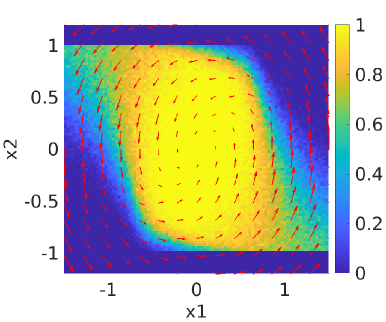
(a) Nominal controller

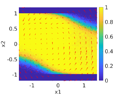
(b) Proposed PIRL

Figure 1: Safety probability for the outlook horizon of $\tau=2.0$.

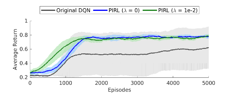
Figure 2: Learning progress.

Benefit of maximally safe policy and probability. Figure 1 shows the safety probability for the outlook horizon $\tau=2.0$ with (a) nominal controller and (b) controller learned by PIRL. Here, the nominal controller was obtained by using the technique of feedback linearization and then applying the LQR theory as in [25]. The safety probabilities in the figure were calculated by a standard Monte Carlo simulation (the estimation accuracy by the function approximator $Q$ will be discussed later). The red arrows in the figure show the vector field of the deterministic part of the dynamics. When the learned policy is used, the system achieves higher safety probability. Thus, when the learned probability is used in probabilistic safety certificates such as [2], it allows the system to explore wider regions.

Efficient learning despite sparse reward. Figure 2 shows the training progress. Besides the plot for the proposed PIRL shown by green, the black line shows the result with the original DQN, and the blue line the PIRL with $\lambda=0$, which means only boundary conditions were imposed. The solid curves correspond to the mean of eight repeated experiments, and the shaded region shows their standard deviation. With the original DQN, the agent has to learn only from sparse zero/one rewards, and often fails to find a safe policy. In contrast, with the proposed PIRL, a safe policy can be found despite the sparse rewards, and the averaged return (corresponds to the safety probability) rises with fewer samples especially at the initial phase.

One of the most common solutions to the issue of sparse reward is reward shaping [27]. For example, one could design a reward $r_{\mathrm{rs}}$ to include information about the distance from the boundary of the safe set:

$$r_{\mathrm{rs}}(s):=r(s)+c(1-x_{2}^{2}).$$ (43)

Figure 3 shows the comparison of the averaged safety probability achieved at the initial phase of the training, where $c=0.05$. It can be seen that the proposed PIRL can learn with fewer experiences as well as the reward shaping. This is because imposing physics loss allows propagation of reward information from neighbors and boundaries, and can serve as an alternative to reward shaping.

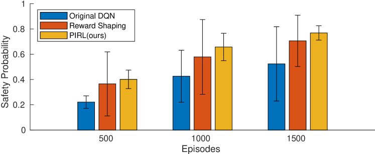
Figure 3: Comparison with reward shaping.

Generalization of PIRL. Figure 4(a) shows the accuracy of the safety probability for $\tau=2.0$ estimated by the function approximater $Q$ learned with $\tau_{\mathrm{D}}\leq\tau$, with and without PDE condition. The bar plot shows the mean squared error between the output of the learned neural network and the Monte Carlo calculation over $10\times 10$ equally distributed points in the state space, and error bar represents its standard deviation over eight repeated experiments. On the other hand, Fig. 4(b) shows the number of unsafe events during the training process with and without the PDE constraint. By reducing $\tau_{\mathrm{D}}$, the number of unsafe events can be reduced, but there is a stringent trade-offs between the estimation accuracy and the length of $\tau_{\mathrm{D}}$ when the PDE constraint is not imposed ($\lambda=0$). In contrast, with the proposed PIRL, the safety probability is accurately estimated without acquiring data no longer than $\tau_{\mathrm{D}}$ while reducing the number of unsafe events. This is beneficial especially in situations when safety must be ensured for a longer period than sampled trajectories and when safe actions must be learned without sufficiently many rare events and unsafe samples.

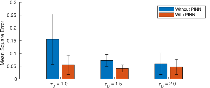
(a) Estimation accuracy for $\tau=2.0$

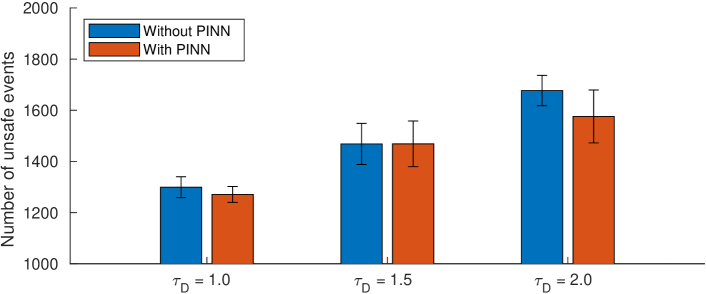
(b) Number of unsafe events

Figure 4: Results of generalization with $\tau_{\mathrm{D}}\leq\tau$.

V Conclusions

In this paper, we proposed a Physics-informed Reinforcement Learning (PIRL) for efficiently estimating the safety probability under maximally safe actions. This was based on the exact characterization of the safety probability as the value function of an RL problem and the derivation of a PDE condition satisfied by the action-value function. The effectiveness of PIRL has been demonstrated through an example based on the Deep Q-Network algorithm integrated with the technique of Physics-informed Neural Network (PINN). Future work includes application of this framework to estimate safety probability in real-world tasks such as autonomous driving, and its use in e.g., safe RL.

APPENDIX

V-A Proof of Proposition 1

Proof.

From the fact that $\tilde{H}_{k}=H_{k}$ and $\tilde{X}_{k}=X_{k}$ hold for $S_{k}\notin\mathcal{S}_{\mathrm{abs}}$, the safety probability $\Psi^{u}(\tau,x)$ can be rewritten as follows:

$$\Psi^{u}(\tau,x)= \mathbb{E}\left[P_{N(\tau)}\,\middle|\,S_{0}=s,u\right]$$ (44)

with the symbol $P_{k}$ is defined as

$$P_{k}:=\prod_{j=0}^{k}\mathds{1}[\tilde{X}_{j}\in\mathcal{C}].$$ (45)

Then, this can be further transformed into a form of sum of multiplicative cost as follows:

$$\Psi^{u}(\tau,x)= \mathbb{E}\bigl{[}\left(P_{N(\tau)}\right)\mathds{1}[\tilde{H}_{N}\in\mathcal{G}]\,\big{|}\,S_{0}=s,u\bigr{]}$$

$$= \mathbb{E}\left[\sum_{k=0}^{N(\tau)}\left(P_{k}\right)\mathds{1}[\tilde{H}_{k}\in\mathcal{G}]\,\middle|\,S_{0}=s,u\right].$$ (46)

Here, the transformations from (44) to (46) is based on the fact that ${\mathds{1}}[\tilde{H}_{k}\in\mathcal{G}]$ is $1$ if $k=N(\tau)$ and $0$ otherwise. Given this form of representation, the proof will be completed by showing that the expectation of the return $G=\sum_{k=0}^{\infty}r(S_{k})$ is equal to (46). First, consider the case where $\tilde{X}_{k}$ stays inside the safe set $\mathcal{C}$ for all $k=0,\dots,N(\tau)$, i.e., the trajectory is safe. In this case, we have

$$P_{k}=1,\quad{\mathds{1}}[S_{k}\notin\mathcal{S}_{\mathrm{abs}}]=1,\quad\forall k\in\{0,\,\dots,\,N(\tau)\}.$$ (47)

Since ${\mathds{1}}[\tilde{H}_{k}\in\mathcal{G}]=0$ for all $k\geq N(\tau)+1$, we have

$$G= \sum_{k=0}^{\infty}{\mathds{1}}[\tilde{H}_{k}\in\mathcal{G}]\,{\mathds{1}}[S_{k}\notin\mathcal{S}_{\mathrm{abs}}]$$

$$= \sum_{k=0}^{N(\tau)}\mathds{1}[\tilde{H}_{k}\in\mathcal{G}]\,{\mathds{1}}[S_{k}\notin\mathcal{S}_{\mathrm{abs}}]$$

$$= \sum_{k=0}^{N(\tau)}\left(P_{k}\right)\mathds{1}[\tilde{H}_{k}\in\mathcal{G}].$$ (48)

Next, consider the case where $\tilde{X}_{\bar{k}}\notin\mathcal{C}$ for some $\bar{k}\in\{0,\dots,N(\tau)\}$, i.e., the trajectory is unsafe. Then, we have

$$P_{k}={\mathds{1}}[S_{k}\notin\mathcal{S}_{\mathrm{abs}}]=1,\quad\forall k\in\{0,\,\dots,\,\bar{k}-1\},$$ (49)

$$P_{k}={\mathds{1}}[S_{k}\notin\mathcal{S}_{\mathrm{abs}}]=0,\quad\forall k\in\{\bar{k},\,\dots,\,N(\tau)\}.$$ (50)

Thus, the return becomes

$$G= \sum_{k=0}^{N(\tau)}\mathds{1}[\tilde{H}_{k}\in\mathcal{G}]\,{\mathds{1}}[S_{k}\notin\mathcal{S}_{\mathrm{abs}}]$$

$$= \sum_{k=0}^{\bar{k}-1}\mathds{1}[\tilde{\tau}_{k}\in\mathcal{G}]+\sum_{k=\bar{k}}^{N(\tau)}0\cdot\mathds{1}[\tilde{H}_{k}\in\mathcal{G}]$$

$$= \sum_{k=0}^{N(\tau)}\left(P_{k}\right)\mathds{1}[\tilde{H}_{k}\in\mathcal{G}].$$ (51)

Thus, the expectation of the return $G$ over all possible trajectories, which is represented either by (48) or (51), is equivalent to the safety probability $\Psi^{u}$ given in (46). Also, the function $v^{u}$ takes a value in $[0,1]$, since the return $G$ takes $0$ or $1$. ∎

V-B Proof of Theorem 1

Proof.

First, consider the following function for the SDE (1) with the exit-time $T_{\mathrm{e}}=\min(T_{\mathcal{C}^{\mathrm{c}}},t_{\mathrm{f}})$:

$$V^{\bar{u}}_{\epsilon}(t_{\mathrm{s}},x):={\mathbb{E}}[l_{\epsilon}(X_{T_{\mathrm{e}}}^{t_{\mathrm{s}},x;\bar{u}})].$$ (52)

Then, it follows from [24, Theorem 4.7] that under Assumption 1(a)-(d), the function $V^{\ast}_{\epsilon}(t_{\mathrm{s}},x):=\sup_{\bar{u}\in\mathcal{U}_{t_{\mathrm{s}}}}V^{\bar{u}}_{\epsilon}(t_{\mathrm{s}},x)$ is a viscosity solution of the following PDE:

$$\sup_{a\in\mathbb{U}}\mathcal{L}^{a}V_{\epsilon}^{\ast}(t_{\mathrm{s}},x)=0, \quad\forall(t_{\mathrm{s}},x)\in[0,t_{\mathrm{f}})\times\mathcal{C},$$ (53)

where $\mathcal{L}^{a}$ is the Dynkin operator defined as

$$\mathcal{L}^{a}\Phi(t,x):= \partial_{t}\Phi(t,x)+f(x,a)^{\top}\partial_{x}\Phi(t,x)$$

$$\quad+\dfrac{1}{2}\text{tr}[\sigma(x,a)\sigma(x,a)^{\top}\partial_{x}^{2}\Phi(t,x)],$$ (54)

and the boundary condition given by

$$V_{\epsilon}^{\ast}(t_{\mathrm{s}},x)=l_{\epsilon}(x),\quad\forall(t,x)\in[0,t_{\mathrm{f}}]\times\mathcal{C}^{\mathrm{c}}\cup\{t_{\mathrm{f}}\}\times\mathbb{R}^{n}.$$ (55)

The continuity of the function $V_{\epsilon}^{\ast}$ follows from Lipschitz continutity of the payoff function $l_{\epsilon}$ and uniform continuity of the stopped solution process [24, Proposition 4.8].

Here, the function $V^{\bar{u}}_{\epsilon}(t_{\mathrm{s}},x)$ can be rewritten as

$$V^{\bar{u}}_{\epsilon}(t_{\mathrm{s}},x) ={\mathbb{E}}[{\mathds{1}}[X_{T_{\mathrm{e}}}^{t_{s},x;\bar{u}}\in\mathcal{C}]\,l_{\epsilon}(X_{T_{\mathrm{e}}}^{t,x;\bar{u}})]$$

$$={\mathbb{E}}[{\mathds{1}}[X_{t}^{t_{s},x;\bar{u}}\in\mathcal{C},\,\forall t\in[t_{\mathrm{s}},t_{\mathrm{f}}]]\,l_{\epsilon}(X_{T_{\mathrm{e}}}^{t,x;\bar{u}})],$$

where the above transformations follows from the fact that $l_{\epsilon}(X_{T_{\mathrm{e}}}^{t_{\mathrm{s}},x;\bar{u}})\neq 0$ only if $X_{T_{\mathrm{e}}}^{t_{\mathrm{s}},x;\bar{u}}\in\mathcal{C}$. Then, with the function $\Psi^{u}_{\epsilon}(\tau,x)$ given by

$$\Psi^{u}_{\epsilon}(\tau,x):=\mathbb{E}\left[\prod_{k=0}^{N(\tau)}{\mathds{1}}[X_{k}\in\mathcal{C}]\,l_{\epsilon}(X_{N(\tau)})~{}\middle|~{}X_{0}=x,u\right],$$

from the continuity of the function $l_{\epsilon}$ and Assumption 1(e), we have $V^{u}_{\epsilon}(t_{\mathrm{f}}-\tau,x)=\lim_{\Delta t\to 0}\Psi^{u}_{\epsilon}(\tau,x)$. Furthermore, with the same arguments as in the proof of Proposition 1, we have $\Psi^{u}_{\epsilon}(\tau,x)=v^{u}_{\epsilon}(s)$ with

$$v^{u}_{\epsilon}(s):=\mathbb{E}\left[\sum_{k=0}^{N(\tau)}r_{\epsilon}(S_{k})~{}\middle|~{}S_{0}=s,u\right].$$ (56)

Since we have

$$v^{u}_{\epsilon}(s)=\max_{a\in\mathbb{U}}q^{\ast}_{\epsilon}(s,a)\xrightarrow[\Delta t\to 0]{}V^{\ast}_{\epsilon}(t_{\mathrm{f}}-\tau,x),$$ (57)

and $V^{\ast}_{\epsilon}(t_{\mathrm{s}},x)$ satisfies the PDE (53), the function $q^{\ast}_{\epsilon}(s,a)$ satisfies the following PDE as $\Delta t\to 0$:

$$\sup_{a\in\mathcal{U}}\partial_{s}q^{\ast}_{\epsilon}(s,a^{\ast})\tilde{f}(s,a)$$

$$\hskip 28.45274pt+\dfrac{1}{2}\mathrm{tr}\left[\tilde{\sigma}(s,a)\tilde{\sigma}(s,a)^{\top}\partial_{s}^{2}q^{\ast}_{\epsilon}(s,a^{\ast})\right]=0.$$ (58)

Here, from $q^{\ast}_{\epsilon}(s,a)=r_{\epsilon}(s)+{\mathbb{E}}[v^{\ast}_{\epsilon}(s^{\prime})|s,a]$, where $s^{\prime}$ is the next state given the current state $s$ and the input $a$, we have

$$a^{\ast} =\operatorname*{arg\,sup}_{a\in\mathbb{U}}\,r(s)+{\mathbb{E}}[v^{\ast}_{\epsilon}(s^{\prime})|s,a]$$

$$=\operatorname*{arg\,sup}_{a\in\mathbb{U}}{\mathbb{E}}[v^{\ast}_{\epsilon}(s^{\prime})|s,a]$$

$$=\operatorname*{arg\,sup}_{a\in\mathbb{U}}\dfrac{{\mathbb{E}}[v^{\ast}_{\epsilon}(s^{\prime})|s,a]-v^{\ast}_{\epsilon}(s)}{\Delta t}$$ (59)

where the above transformation is based on the fact that $r_{\epsilon}(s)$ and $v^{\ast}_{\epsilon}$ are independent of $a$. Thus, from the Ito’s Lemma, $a^{\ast}$ maximizes the right-hand side of (V-B) as $\Delta t\to 0$, and substituting $a^{\ast}$ gives (27):

$$\partial_{s}q^{\ast}_{\epsilon}(s,a^{\ast})\tilde{f}(s,a^{\ast})$$

$$\hskip 14.22636pt+\dfrac{1}{2}\mathrm{tr}\left[\tilde{\sigma}(s,a^{\ast})\tilde{\sigma}(s,a^{\ast})^{\top}\partial_{s}^{2}q^{\ast}_{\epsilon}(s,a^{\ast})\right]=0.$$

∎

References

• [1] M. P. Chapman, J. Lacotte, A. Tamar, D. Lee, K. M. Smith, V. Cheng, J. F. Fisac, S. Jha, M. Pavone, and C. J. Tomlin, “A risk-sensitive finite-time reachability approach for safety of stochastic dynamic systems,” in 2019 American Control Conference (ACC), 2019, pp. 2958–2963.
• [2] Z. Wang, H. Jing, C. Kurniawan, A. Chern, and Y. Nakahira, “Myopically verifiable probabilistic certificate for long-term safety,” in 2022 American Control Conference (ACC), Jun. 2022, pp. 4894–4900.
• [3] F. M. F. Berkenkamp, “Safe exploration in reinforcement learning: Theory and applications in robotics,” Ph.D. dissertation, ETH Zurich, 2019.
• [4] Y. Kim, R. Allmendinger, and M. López-Ibáñez, “Safe learning and optimization techniques: Towards a survey of the state of the art,” in Trustworthy AI - Integrating Learning, Optimization and Reasoning.   Springer International Publishing, 2021, pp. 123–139.
• [5] K. Srinivasan, B. Eysenbach, S. Ha, J. Tan, and C. Finn, “Learning to be safe: Deep RL with a safety critic,” arXiv: 2010.14603 [cs.LG], Oct. 2020.
• [6] Z. Qin, Y. Chen, and C. Fan, “Density constrained reinforcement learning,” in Proceedings of the 38th International Conference on Machine Learning, 2021, pp. 8682–8692.
• [7] W. Chen, D. Subramanian, and S. Paternain, “Policy gradients for probabilistic constrained reinforcement learning,” in 57th Annual Conference on Information Sciences and Systems, 2023, pp. 1–6.
• [8] B. Thananjeyan, A. Balakrishna, S. Nair, M. Luo, K. Srinivasan, M. Hwang, J. E. Gonzalez, J. Ibarz, C. Finn, and K. Goldberg, “Recovery RL: Safe reinforcement learning with learned recovery zones,” Oct. 2020.
• [9] J. Zhang, “Modern monte carlo methods for efficient uncertainty quantification and propagation: A survey,” WIREs Computational Statistics, vol. 13, no. 5, p. e1539, 2021.
• [10] J. F. Fisac, N. F. Lugovoy, V. Rubies-Royo, S. Ghosh, and C. J. Tomlin, “Bridging Hamilton-Jacobi safety analysis and reinforcement learning,” in 2019 International Conference on Robotics and Automation (ICRA), May 2019, pp. 8550–8556.
• [11] A. Tamar, Y. Chow, M. Ghavamzadeh, and S. Mannor, “Policy gradient for coherent risk measures,” Adv. Neural Inf. Process. Syst., vol. 28, 2015.
• [12] A. Abate, M. Prandini, J. Lygeros, and S. Sastry, “Probabilistic reachability and safety for controlled discrete time stochastic hybrid systems,” Automatica, vol. 44, no. 11, pp. 2724–2734, Nov. 2008.
• [13] M. Raissi, P. Perdikaris, and G. E. Karniadakis, “Physics-informed neural networks: A deep learning framework for solving forward and inverse problems involving nonlinear partial differential equations,” J. Comput. Phys., vol. 378, pp. 686–707, Feb. 2019.
• [14] S. Cai, Z. Mao, Z. Wang, M. Yin, and G. E. Karniadakis, “Physics-informed neural networks (PINNs) for fluid mechanics: a review,” Acta Mech. Sin., vol. 37, no. 12, pp. 1727–1738, Dec. 2021.
• [15] S. Cuomo, V. S. Di Cola, F. Giampaolo, G. Rozza, M. Raissi, and F. Piccialli, “Scientific machine learning through Physics–Informed neural networks: Where we are and what’s next,” J. Sci. Comput., vol. 92, no. 3, p. 88, Jul. 2022.
• [16] Z. Wang and Y. Nakahira, “A generalizable physics-informed learning framework for risk probability estimation,” in Proceedings of the 5th Annual Learning for Dynamics and Control Conference (L4DC), 2023, pp. 358–370.
• [17] V. Mnih, K. Kavukcuoglu, D. Silver, A. Graves, I. Antonoglou, D. Wierstra, and M. Riedmiller, “Playing atari with deep reinforcement learning,” arXiv: 1312.5602 [cs.LG], Dec. 2013.
• [18] C. Banerjee, K. Nguyen, C. Fookes, and M. Raissi, “A survey on physics informed reinforcement learning: Review and open problems,” arXiv: 2309.01909 [cs.LG], Sep. 2023.
• [19] W. H. Fleming and H. M. Soner, Controlled Markov Processes and Viscosity Solutions, 2nd ed.   Springer, 2006.
• [20] X. Mao, “Stabilization of continuous-time hybrid stochastic differential equations by discrete-time feedback control,” Automatica, vol. 49, no. 12, pp. 3677–3681, 2013.
• [21] E. Bayraktar and A. D. Kara, “Approximate q learning for controlled diffusion processes and its near optimality,” SIAM Journal on Mathematics of Data Science, vol. 5, no. 3, pp. 615–638, 2023.
• [22] S. Summers and J. Lygeros, “Verification of discrete time stochastic hybrid systems: A stochastic reach-avoid decision problem,” Automatica, vol. 46, no. 12, pp. 1951–1961, Dec. 2010.
• [23] R. S. Sutton and A. G. Barto, Reinforcement Learning: An Introduction, 2nd ed.   Cambridge, MA: MIT Press, 2018.
• [24] P. Mohajerin Esfahani, D. Chatterjee, and J. Lygeros, “The stochastic reach-avoid problem and set characterization for diffusions,” Automatica, vol. 70, pp. 43–56, 2016.
• [25] R. W. Beard, G. N. Saridis, and J. T. Wen, “Galerkin approximations of the generalized hamilton-jacobi-bellman equation,” Automatica, vol. 33, no. 12, pp. 2159–2177, 1997.
• [26] V. Rubies-Royo, D. Fridovich-Keil, S. Herbert, and C. J. Tomlin, “A classification-based approach for approximate reachability,” in 2019 International Conference on Robotics and Automation (ICRA), May 2019, pp. 7697–7704.
• [27] Nilaksh, A. Ranjan, S. Agrawal, A. Jain, P. Jagtap, and S. Kolathaya, “Barrier functions inspired reward shaping for reinforcement learning,” arXiv: 2403.01410 [cs.RO], 2024.