Illuminating Systematic Trends in Nuclear Data with Generative Machine Learning Models

Abstract

We introduce a novel method for studying systematic trends in nuclear reaction data using generative adversarial networks. Libraries of nuclear cross section evaluations exhibit intricate systematic trends across the nuclear landscape, and predictive models capable of reproducing and analyzing these trends are valuable for many applications. We have developed a predictive model using deep generative adversarial networks to learn trends from the inelastic neutron scattering channel of TENDL for even-even nuclei. The system predicts cross sections based on adding/subtracting particles to/from the target nucleus. It can thus help identify cross sections that break from expected trends and predict beyond the limit of current experiments. Our model can produce good predictions for cross section curves for many nuclides, and it is most robust near the line of stability. We also create an ensemble of predictions to leverage different correlations and estimate model uncertainty. This research marks an important first step in computer generation of nuclear cross-section libraries.

I Introduction

I.1 Nuclear cross section evaluations

Simple patterns and trends have long been a staple in the phenomenology of atomic nuclei. The values that nuclear masses take as functions of the number of protons (Z) and neutrons (N) are one of the best-studied cases of such trends. Despite the rich and complex quantum many-body structure that enters a precise description of nuclear ground states, their masses are well described by simple semi-empirical formulae, such as a liquid drop model [1], which captures the dependence of nuclear masses in terms of total number of nucleons ($N+Z$), asymmetry between protons and neutrons ($N-Z$), and corrections for effects such as pairing. More recent studies exploit trends related to static properties (nuclear skins, electromagnetic transition strengths, etc.) to build ensembles of nuclear models (or ensembles of parameterizations of a specific model) and connect predictions to experimental measurements [2, 3]. This work has a slightly different aim. Instead of looking at relatively simple data with prominent trends or looking at the pattern between purely theoretical models, we seek to learn about trends hidden in libraries of evaluated nuclear reaction cross sections.

Evaluated nuclear reaction data, such as the ENDF[4], JEFF[5], or TENDL[6] libraries (non-exhaustively), represents the interface between nuclear physics and other sciences and engineering that depend on nuclear physics. The consumers of nuclear data span from astrophysical simulations and high energy physics (through detector/background design and modeling) to nuclear power, safety, and radiological medicine [7]. These evaluated libraries are a fusion of experimental data and theoretical models that aim to give a comprehensive picture of scattering processes for as much of the nuclear chart as possible. Present in these libraries are complicated systematic trends due to fundamental nuclear physics, but these can be difficult to study due to the tremendous size of these libraries and their density of information, and the complexity of reaction cross sections. From a theoretical perspective, the whole libraries are not presently well described by a singular model, and instead, a patchwork of different models are combined locally (in proton and neutron numbers) across the chart, obfuscating these trends. Our goal for this work is to develop a machine learning system to facilitate analysis of trends in cross sections and, using existing evaluation libraries, predict cross sections beyond experimental barriers.

We focus on the TENDL library [6] and the inelastic neutron scattering channel $(n,n^{\prime})$ in particular, with resonances excluded; this choice was made because of the relative simplicity of correlations in this channel. Because of odd-even staggering, the well-known behavior of systematic trends in nuclei to oscillate with parity of proton/neutron numbers $Z,N$, we only work with even-even nuclei in the present study. While this significantly reduces the complexity of trends the model must learn, it nonetheless requires a model with sufficiently large complexity to make reasonable predictions. This simplification makes it much easier to interpret results and better develop our approach; this work is a foundation for developing more sophisticated models.

This data set has many different types of correlations (i.e., at different scales over the chart of nuclides), making it a ripe target for data science and machine learning. For instance, a predictive model must learn correlations in the cross sections between values of scattering energy, correlations between nuclei with similar numbers of constituent particles, and (in future development) correlations between cross sections in different reaction channels.

Recent advances in artificial intelligence applications to nuclear physics have been numerous and broad in scope [8, 9, 10, 11]. The present work is most similar to data-driven methods for nuclear masses [12, 13, 14] and error detection in engineering libraries [15], but significant progress has also been made on ML (including neural network) applications to the many-fermion problem [16, 17, 18].

I.2 High-level model summary

Our deep learning model has two main components working in tandem: a variational auto-encoder (VAE), responsible for encoding the cross section evaluation in a dense representation, and the generative adversarial network (GAN), responsible for transforming the dense representation for one nuclide to that of a nearby nuclide.

First, the VAE encodes the cross sections from TENDL, which we have numerically standardized (0-30 MeV) and normalized. This produces an encoded data set, where each cross section is represented by a vector. We append to each vector a linear transform of $(N,Z)$ to help the GAN distinguish similar vectors. These vectors are then paired up according to neighboring nuclides: those which differ in $Z$ or $N$ by at most 2. The GAN is trained to transform each vector to the corresponding neighbor. The result can then be decoded by the VAE to predict the cross section curve at the target nuclide. Lastly, we devote a separate identical GAN model to each of the four linear “files” across the chart of nuclides ($\updownarrow,\neswarrow,\leftrightarrow,\nwsearrow$; each corresponding to a fixed change in $(Z,N)$).

The full predictive system is thus an ensemble, which has advantages and disadvantages. Cross sections of any nuclide can be predicted by starting at one nuclide and convolving the necessary transformations. We can make predictions for cross sections of nuclides inside and outside the training region by combining predictions using many paths across the chart, allowing for the entire model to be utilized in each prediction. We hypothesize that this model can be used in this way to illuminate systematic trends in nuclear data libraries and make predictions for cross sections for which experimental measurements do not exist.

II A Predictive AI model for cross section curves

II.1 The convolutional variational auto-encoder (VAE)

The first step in our procedure, typical for machine learning tasks, is to find an ideal representation of the data. This includes normalization and an encoding to simplify correlations in the data and reduce dimension. We standardize cross sections to lie on a fixed energy domain of $0-30$ MeV in 256 bins and normalize them individually to a maximum of 1. This way, we factor out the task of predicting amplitudes and just focus on the shape of the curve. In principle, the scales could be included in the predictive model in future development, but that would likely require some non-trivial modification of the VAE encoding process.

One powerful method of data encoding uses a neural network model called an auto-encoder (AE), which can be thought of as a nonlinear principal component analysis (PCA). When doing linear PCA via singular value decomposition (SVD), one finds orthogonal principal components of data, and the whole data set can be represented using those components as a basis. A standard procedure for data encoding with SVD is to drop the basis components with small singular values and represent all data with the remaining components. Thus, one may efficiently represent the data in a smaller dimension. PCA ensures that components with small singular values are the least important, so ignoring them introduces as little error as possible. However, linear PCA includes some crucial assumptions about the data: the data is a linear combination of explanatory variables, all explanatory variables have been observed roughly the same amount, correlations follow a Gaussian distribution, the data is primarily unimodal, etc. Furthermore, cross sections are strictly positive, and using linear PCA to reduce dimension inevitably produces negative cross sections. For these reasons, a neural network auto-encoder is a more robust encoding method for this problem. Fig. 1 illustrates the improved compression capability of the VAE over linear PCA (using the same number of variables).

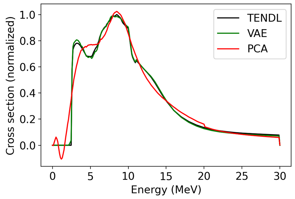
Figure 1: Comparison of cross section evaluation data compression. The variational auto-encoder outperforms a linear principle component analysis with the same number of variables.

An AE model is a neural network mapping from data $\Sigma$ to itself, and the smallest layer inside the network is the latent space representation of the input. The model is split into an encoder part $E$ before the latent layer and a decoder part $E^{+}$ after the latent layer (borrowing notation from the Moore-Penrose pseudoinverse). The AE model can be nicely represented as a function convolution, $E^{+}(E(\sigma))=\sigma^{\prime}$. With weights $\theta$ and $\theta^{+}$ for $E$ and $E^{+}$, respectively, the simplest loss function penalizes errors over a batch of $N_{b}$ data as follows.

$$\mathcal{L}_{\text{AE}}(\theta,\theta^{+};\Sigma)=\frac{1}{N_{b}}\sum_{i=1}^{N_{b}}|E^{+}_{\theta^{+}}(E_{\theta}(\sigma_{i}))-\sigma_{i}|^{2}$$ (1)

Thus, $E^{+}$ approaches $E^{-1}$ as the loss function is minimized, meaning the encoder and decoder transform to and from the latent space.

One problem that arises with the simple AE is that we do not have any control over the distribution of latent space encodings, and this is undesirable because we plan to use these encodings as input for another model. Having a smooth and efficient encoding is a high priority, so we turn to a more appropriate formulation of the encoding problem: variational Bayes (VB) and, in particular, the VAE. VB refers to statistical methods that approximate a probability distribution with a conditional (or joint) one, often using Kullback-Leibler divergence (KLD) as a distance metric. In the present case, we want to approximate the distributions $P_{E(\theta)}(z|\sigma)$, the encoding, and $P_{E^{+}(\theta^{+})}(\sigma^{\prime}|z)$, the decoding. In essence, the VAE maps the VB problem onto the auto-encoder neural network structure: the problem has a robust statistical foundation, and we introduce deep neural networks to learn the probability distributions. When the VAE networks are converged, we can encode all input data into the latent space representation, $E(\Sigma)=Z$, and the rest of the model will work entirely on the encoded data $Z$.

In what is known as the reparameterization trick, the VAE maps the latent variables to parameters of Gaussian distributions rather than points. This means the latent representation of $\sigma$ used in the VAE is not $E(\sigma)=z$ but rather $E(\sigma)=(m_{z},s^{2}_{z})$, where $m_{z}$ and $s^{2}_{z}$ are the mean and variance assigned by the model to data point $z$. When training the VAE, the latent representation is a random sample from $\mathcal{N}(m_{z},s_{z}^{2})$. Each latent space representation $z$ is mapped to output $x^{\prime}$ according to the probability distribution $P(E(\sigma))=\mathcal{N}(m_{z},s^{2}_{z})$. When using the VAE for encoding after training, the random noise is removed, so the encoding is deterministic $E(\sigma)=m_{z}$, and so we typically denote the encoded data $m_{z}=z$ as before.

The VAE loss function combines the AE loss and VB loss: Kullback-Leibler divergence (KLD) plus reconstruction error.

$$\mathcal{L}_{\text{VAE}}(\theta,\theta^{+};\Sigma) =-\frac{1}{N_{b}}\sum_{i=1}^{N_{b}}\text{KLD}\left[P_{E(\theta)}(z|\sigma_{i})||\mathcal{N}(m_{z},s^{2}_{z})\right]$$ (2)

$$+\mathcal{L}_{\text{AE}}(\theta,\theta^{+};\Sigma)$$

The function $\text{KLD}(P||P^{\prime})$ essentially measures the difference between distributions $P$ and $P^{\prime}$. In our case, where the comparison is made to a Gaussian distribution, this function reduces nicely to the following.

$$\text{KLD}_{\beta}\left[P_{E(\theta)}(z|\sigma)||\mathcal{N}(m_{z},s^{2}_{z})\right]=\frac{\beta}{2}\left[1+\log s_{z}^{2}-m_{z}^{2}-s_{z}^{2}\right]$$ (3)

The scale of the KLD loss term in the total loss function is parameterized by the number $\beta$, which, in practice, may be changed during training. With a sufficiently complex neural network, it is easy to find (via numerical optimization with stochastic gradient descent) a minimization of KLD with large reconstruction error: in other words, the latent space representations are Gaussian, but $E$ and $E^{+}$ are not good approximations to the distributions they should be learning. To help this, a good trick is to schedule the KLD $\beta$ to oscillate from 0 to 1 a few times before ultimately fixing it to 1. In our case, this resulted in good convergence and is especially easy to implement in code.

In addition, the VAE’s encoding and decoding layers are fully convolutional. Cross sections have strong short-range correlations and weak long-range correlations; in other words, the covariance matrix is diagonally dominant. We leverage this property by using convolutional layers in the VAE neural networks, which learn multi-scale correlations; each consecutive hidden layer is responsible for a slightly larger or smaller correlation length. This is similar to AI models used for image recognition: long-range correlations are not ignored, but the relative importance of short-range correlations is built directly into the network architecture. A convolutional neural network is likely superior to the usual densely connected feed-forward neural network for data dominated by local correlations, especially for a use-case like encoding. This is especially true in complicated problems where larger neural networks are employed; for a fixed number of layers, the convolutional network has fewer parameters than the dense one and, thus, is generally easier to train.

The combination of convolutional layers and learning VB results in an efficient mapping to the latent space: it appears that large-scale features in the cross section are provided large $s_{z}^{2}$ and are smoother with respect to the latent space, and smaller-scale features are given a smaller $s_{z}^{2}$. So, the latent space appears to naturally reflect the trends present in the data.

II.2 Generative adversarial networks (GANs)

We employ a generative adversarial network (GAN) to learn trends in the cross sections. Before introducing the GAN, it is worth mentioning that deep generative learning (and the subset of it which is adversarial) as a field of study has expanded and matured significantly in the years since the first GAN work was published [19]. In the present research, we have developed our architecture based on experience with the relevant physics, but there are many different types of GAN models one may consider for this task [20, 21, 22, 23, 24]. We cannot possibly give a comprehensive description of all the ways a GAN may be applied to nuclear data. Our model is the result of over two years of ongoing study and development, but it is not a perfect solution, and we hope that this work will prompt other researchers to develop more creative and effective methods for these sorts of problems.

A brief introduction to simple GANs is provided in Appendix A.

II.2.1 Cycle-consistent GANs

Zhu et al. [25] demonstrated the effectiveness of cycle-consistent GANs (cycleGANs) for image-to-image translation: two GANs $\{G,D_{G}\}$ and $\{F,D_{F}\}$, may be used to map between two distinct probability distributions, for $x\in X$ and $y\in Y$, as $G(x)=y^{\prime}\;\tilde{\in}\;Y$ and $F(y)=x^{\prime}\;\tilde{\in}\;X$ (read: $y^{\prime}$ is similar to elements of $Y$, etc.). The discriminator networks $D_{G}$ and $D_{F}$ score the validity of the two resulting candidates: $D_{G}(y^{\prime})=P(y^{\prime}\in Y|y\in Y)$ and $D_{F}(x^{\prime})=P(x^{\prime}\in X|x\in X)$. The cycleGAN loss functions add two new terms to the loss functions in Eq. 18. First, cycle loss ensures that applying the generators in succession returns the input (i.e., the convolution of co-inverse generators is the identity function). For a batch of $N_{b}$ data points, cycle loss is as follows.

$$\mathcal{L}^{G}_{\text{cycle}}=\frac{1}{N_{b}}\sum_{i}^{N_{b}}|X_{i}-F(G(X))_{i}|+\frac{1}{N_{b}}\sum_{i}^{N_{b}}|Y_{i}-G(F(Y))_{i}|$$ (4)

One such application is style transfer [20] where $G$ learns to transform $X$ so that correlations match those of $Y$, and $F$ learns the reverse. Style transfer employs the constraint that generators be idempotent ($G^{2}=G$): $G(y)\;\tilde{\in}\;Y$ and $F(x)\;\tilde{\in}\;X$ because the generators should act as projections into the respective spaces (that is, $G(x)\;\tilde{\in}\;Y$ but $G(G(x))\;\tilde{\in}\;Y$ as well). The term “cycle-consistent” refers to an additional constraint that each generator be the inverse of its partner: $G(F(y))=G(x^{\prime})=y^{\prime}$ and $F(G(x))=F(y^{\prime})=x^{\prime}$. This is one of several mechanisms that encourage the generators to learn systematic trends rather than simply “memorize” the training data (e.g., network configurations that only serve one purpose). We can denote such a cycleGAN system as the set $\{G,F,D_{G},D_{F}\}$.

II.2.2 The cycleGAN for cross section curves

Our method for transforming cross-sections is a modified version of the cycleGAN for style transfer: we rely on cycle consistency, but there are some important differences. First, our data is paired, so we do not use the projection constraint present in style transfer. Having generators be projectors makes sense in style transfer because there are two distinct distributions being mapped between, but we want the generators to learn changes based on changing proton/neutron numbers which will always have some effect on the cross section. Our generators map between data points within a single domain, and consequently, we have a single shared discriminator $D_{G}=D_{F}=D$. We denote the modified cycleGAN as $\{G,F,D\}$.

Second, we introduce a new loss term: target loss, equal to the traditional mean absolute error between the model and target cross section. Without this constraint, the total loss function would contain local minima not relevant to the physical solution. (An identity transformation, for instance, satisfies cycle loss but does not correspond to physics.) The total loss function is thus biased toward the particular solution to the adversarial GAN problem that reproduces the physics. We introduce a tunable parameter $\lambda_{\text{target}}$ for controlling the weight of target loss, which is scheduled to be large at the beginning of training so the optimizer converges quickly, then drops later in training so as not to overfit.

$$\mathcal{L}^{G}_{\text{target}}=\frac{1}{N_{b}}\sum_{i}^{N_{b}}|X_{i}-F(Y)_{i}|+\frac{1}{N_{b}}\sum_{i}^{N_{b}}|Y_{i}-G(X)_{i}|$$ (5)

The GAN overfitting problem is subtle and challenging, in part because it is quite different from overfitting in simple regression models, which is very well understood. A typical regression problem abides by the Gauss-Markov assumptions: the distribution of errors between the model and target has zero mean and a diagonal (or at least diagonally dominant) covariance matrix. This assumption does not hold for the present approach: cross section evaluations are, in some cases, much more detailed than others, different evaluations may involve different theoretical models and experimental factors, and the library may even include some mistakes. This makes it very difficult to make any assumptions about the form of the covariance matrix of errors. What we can do, however, is control overfitting via model complexity, regularization, and by tuning $\lambda_{\text{target}}$.

We judge overfitting based on evaluations for validation data, as in a typical regression problem: we assume that when errors on validation data are approximately equal to those on training data, locally, the probability of having overfit is low. The converse, however, is not true: a low probability of local overfitting does not necessarily mean that errors on validation data are approximately equal to those on nearby training data. The TENDL library contains some individual cross section evaluations (e.g. ¹²C) that have been finely tuned to experimental data while surrounding cross sections have not. Thus, if that cross section is held out for validation, we cannot always expect the model to predict those details. In short, the model cannot predict a systematic relation between cross sections that is not present in the training data across multiple nuclides.

Regularization of the neural networks is implemented in two ways: dropout and label noise. Dropout is used in both the generators and the discriminator. During training, upon each iteration, some percentage of neurons are randomly chosen to turn off, outputting zero. This makes network predictions more robust since no single neuron can be relied on all of the time, making it much less likely that the network will “memorize” data. We use a dropout probability of 50% on the inner hidden layers of the generators and 25% for the discriminator; hidden layers near the input and output do not use dropout. Label noise is a regularization tool that works on the discriminator; rather than using labels 0 or 1 for all training data, a small random $\epsilon$ is chosen and added/subtracted to the label accordingly. That is, upon every iteration we choose $\epsilon\sim\mathcal{N}(0,\sigma_{\epsilon}^{2})$ and then replace $0\rightarrow 0+|\epsilon|$ and $1\rightarrow 1-|\epsilon|$. The standard deviation $\sigma_{\epsilon}$ is 0.1 in the present application (this value was not arrived at via any optimization, and in general, such an exploration may be warranted). This has the effect of smoothing the discriminator predictions around the limits, keeping the discriminator from assigning probabilities “overconfidently”, so to speak. It is generally common to have label noise applied to only one label (i.e., either 0 or 1, not both); however, in the present work, we found applying the noise to both gave better results.

II.3 The ensemble of cycleGAN models on the chart of nuclides

Our full predictive model consists of four copies of the above-mentioned cycleGAN model. We now introduce some notation to clarify this section. The chart of nuclides is oriented with $N$ on the horizontal axis and $Z$ on the vertical. First, for individual directions on the chart of nuclides (cardinals and diagonals), we use the symbol $d\in\{\uparrow,\nearrow,\rightarrow,\searrow,\downarrow,\swarrow,\leftarrow,\nwarrow\}$. Second, we use the symbol $f$ for “file”, meaning each pair of co-inverse directions, so $f\in\{\updownarrow,\neswarrow,\leftrightarrow,\nwsearrow\}$. Each of the four cycleGANs corresponds to a file, and thus a physical change in $(N,Z)$: the $\leftrightarrow$ file corresponds to adding/subtracting neutron pairs, the $\updownarrow$ file to adding/subtracting proton pairs, the $\neswarrow$ file to adding/subtracting both proton and neutron pairs (a.k.a. isoscalar) and the $\nwsearrow$ file to swapping a proton pair for neutron pair and vice versa (a.k.a. isovector). Denoting each cycleGAN set as $M$, we can denote the four separate models in Eq. 6. The subscript direction of generators $G,F$ indicates the transform each has learned.

$$M_{\leftrightarrow} =\{G_{(N,Z)\rightarrow(N+2,Z)},F_{(N,Z)\rightarrow(N-2,Z)},D_{\leftrightarrow}\}$$ (6)

$$M_{\updownarrow} =\{G_{(N,Z)\rightarrow(N,Z+2)},F_{(N,Z)\rightarrow(N,Z-2)},D_{\updownarrow}\}$$

$$M_{\neswarrow} =\{G_{(N,Z)\rightarrow(N+2,Z+2)},F_{(N,Z)\rightarrow(N-2,Z-2)},D_{\neswarrow}\}$$

$$M_{\nwsearrow} =\{G_{(N,Z)\rightarrow(N+2,Z-2)},F_{(N,Z)\rightarrow(N-2,Z+2)},D_{\nwsearrow}\}$$

However, for simplicity, we rename the generator networks to $T_{d}$ with a subscript arrow indicating the direction of transformation on the chart of nuclides.

$$M_{\leftrightarrow} =\{T_{\rightarrow},T_{\leftarrow},D_{\leftrightarrow}\}$$ (7)

$$M_{\updownarrow} =\{T_{\uparrow},T_{\downarrow},D_{\updownarrow}\}$$

$$M_{\neswarrow} =\{T_{\nearrow},T_{\swarrow},D_{\neswarrow}\}$$

$$M_{\nwsearrow} =\{T_{\searrow},T_{\nwarrow},D_{\nwsearrow}\}$$

To further simplify notation, consider the file $f$ corresponding to co-inverse directions $d$ and $\bar{d}$. Then, $M_{f}=\{T_{d},T_{\bar{d}},D_{f}\}$.

Let $\Sigma$ with no subscript mean the set of all normalized TENDL $(n,n^{\prime})$ cross section evaluations, $\Sigma=\{\sigma_{(N,Z)}\}$. For each cycleGAN, a set of training cross section curves $\Sigma_{f}$ is prepared by pairing cross sections along the relevant file. Sets of pairs of cross sections are denoted as follows.

$$\Sigma_{\leftrightarrow} =\{(\sigma_{(N,Z)},\sigma_{(N+2,Z)})\}$$ (8)

$$\Sigma_{\updownarrow} =\{(\sigma_{(N,Z)},\sigma_{(N,Z+2)})\}$$

$$\Sigma^{\prime}_{\neswarrow} =\{(\sigma_{(N,Z)},\sigma_{(N+2,Z+2)})\}$$

$$\Sigma_{\nwsearrow} =\{(\sigma_{(N,Z)},\sigma_{(N+2,Z-2)})\}$$

Preparation of data for the GAN follows in two steps. First, we use the VAE to encode each element of $\Sigma$, $E(\sigma_{(N,Z)})=z_{(N,Z)}$, which forms the full encoded data set $\mathcal{Z}$. The sets of encoded cross section pairs corresponding to each model are denoted similarly with $\mathcal{Z}_{f}$.

$$\mathcal{Z}_{\leftrightarrow} =\{(z_{(N,Z)},z_{(N+2,Z)})\}$$ (9)

$$\mathcal{Z}_{\updownarrow} =\{(z_{(N,Z)},z_{(N,Z+2)})\}$$

$$\mathcal{Z}_{\neswarrow} =\{(z_{(N,Z)},z_{(N+2,Z+2)})\}$$

$$\mathcal{Z}_{\nwsearrow} =\{(z_{(N,Z)},z_{(N+2,Z-2)})\}$$

Secondly, each vector $z_{(N,Z)}$ is appended with normalized values of proton and neutron number $N,Z$. We can denote the resulting form of our data as $\tilde{\mathcal{Z}}_{f}$, every element of which is a pair of encoded cross sections appended with normalized proton/neutron numbers, i.e. $(\tilde{z}_{(N,Z)},\tilde{z}_{(N,Z)+d})\in\tilde{\mathcal{Z}}_{f}$. As such, the dimension of the generator input/output is equal to the VAE latent dimension plus 2. While we did not find it necessary to introduce, other neural network models for nuclear data [13] have shown clear improvements in convergence when redundant physical information is included as additional features ($N-Z$,$A^{1/3}$, etc.).

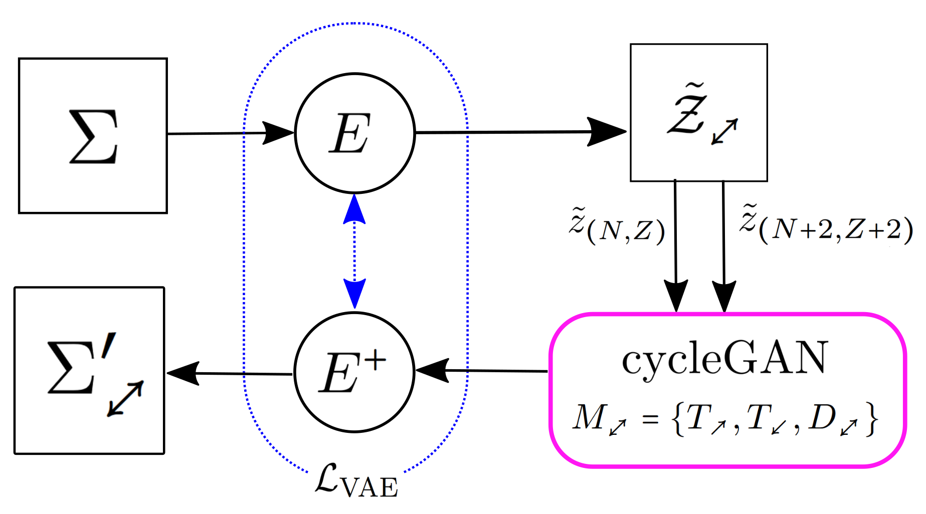
(a) The normalized cross section data $\Sigma$ is first encoded $E$ and appended with numbers $(N,Z)$ to form the training set $\tilde{\mathcal{Z}}_{\neswarrow}$, which is fed to the cycleGAN. The corresponding encoded predictions $\tilde{\mathcal{Z}}^{\prime}_{\neswarrow}$ are then decoded ($E^{+}$), which provides predictions of cross section curves $\Sigma^{\prime}_{\neswarrow}$.

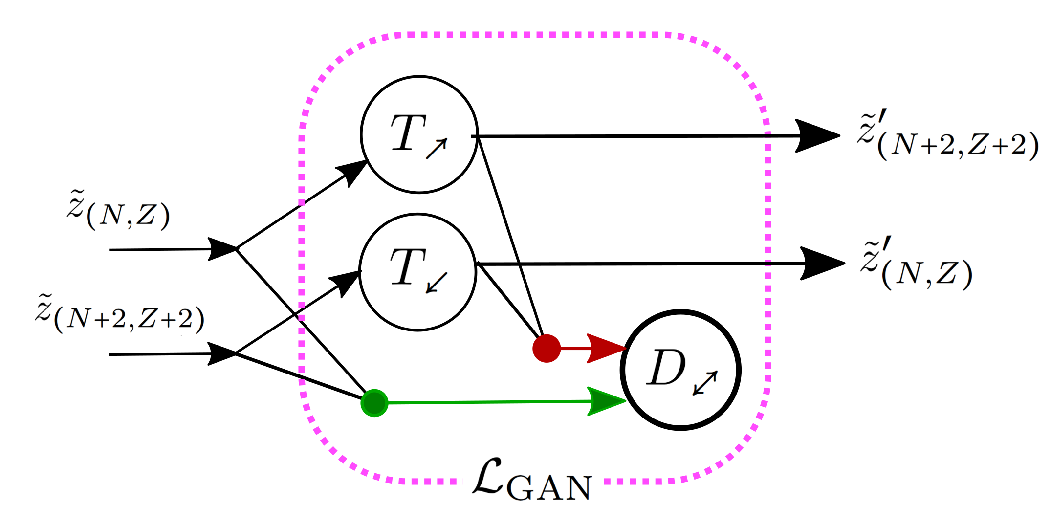
(b) The cycleGAN model accepts the pair of encoded vectors, $\tilde{z}_{(N,Z)}$ and $\tilde{z}_{(N+2,Z+2)}$ without loss of generality. The pair is concatenated to provide the discriminator $D_{\neswarrow}$ a sample of “real” data. Each vector is then transformed by the respective generator model $T_{\nearrow},T_{\swarrow}$; this pair is concatenated to provide the discriminator with a sample of “fake” data.

Figure 2: Flowcharts illustrating prediction procedure using the VAE and cycleGAN. The notation shown corresponds to the $\neswarrow$ file on the nuclear chart; without loss of generality, each model has the same structure ($\updownarrow,\neswarrow,\leftrightarrow,\nwsearrow$).

Note that the discriminator networks have a different job than in a cycleGAN used for style-transfer. Rather than accept a single data vector $\tilde{z}$ and determine $P(\tilde{z}\in\tilde{\mathcal{Z}})$, the discriminator $D_{f}$ accepts an ordered pair $(\tilde{z}_{(N,Z)},\tilde{z}_{(N,Z)+d})$ and learns $P((\tilde{z}_{1},\tilde{z}_{2})\in\tilde{\mathcal{Z}}_{f})$. The order of the pair matters, so discriminator $D_{f}$ should assign 1 to (that is, accept) only pairs of vectors that together match the distribution of variables along file $f$ in the data. (Data sets are constructed using all possible pairs, so $\{(\tilde{z}_{(N,Z)},\tilde{z}_{(N,Z)+d})\}$ is synonymous with $\{(\tilde{z}_{(N,Z)+\bar{d}},\tilde{z}_{(N,Z)})\}$.)

III Optimization

Each model $M_{a}$ is trained by iterating over a subset of $\tilde{\mathcal{Z}}_{f}$, computing the value of a loss function for each pair (sometimes a batch of pairs), and adjusting network weights according to a minimization algorithm. The loss function for each cycleGAN has four main components: cycle-consistency losses, prediction losses, and the two adversarial losses. Without loss of generality, we write the loss function for a single cycleGAN $\{G,F,D\}$ as follows.

$$\mathcal{L}_{\text{GAN}}=\lambda_{\text{cycle}}\mathcal{L}^{G}_{\text{cycle}}+\lambda_{\text{target}}\mathcal{L}^{G}_{\text{target}}+\lambda_{\text{fake}}\mathcal{L}^{D}_{\text{fake}}+\lambda_{\text{real}}\mathcal{L}^{D}_{\text{real}}$$ (10)

The coefficients are determined simply by trial and error, we found that $\lambda_{\text{cycle}}=1,\lambda_{\text{fake}}=\lambda_{\text{real}}=1$ worked well for this case. The target loss coefficient $\lambda_{\text{target}}$ is set larger (e.g., 5-10) at the beginning of training, then scheduled to decrease to 1. This brings the system to the relevant region of parameter space early, after which we may relax the constraint that predictions match very closely with TENDL data.

We use a translated and scaled sigmoid function to do schedule changes in values while training. The following function $S_{m,s}(t)$ begins at $S_{i}$, and, in the window between times $t_{i}$ and $t_{f}$, gradually approaches the value $S_{f}$. The parameters $m$ and $s$ control the translation and scale (in time), respectively.

$$S_{m,s}(t)=\begin{cases}S_{i}&t<t_{i}\\ S_{i}+\frac{S_{f}-S_{i}}{1+\exp\left[{-(t-m)/s}\right]}&t_{i}<t<t_{f}\\ S_{f}&t>t_{f}\\ \end{cases}$$ (11)

This function is used to schedule the decrease in learning rate and $\lambda_{\text{target}}$. The initial and final epochs $t_{i},t_{f}$ depend on convergence but are on the order of 10,000 epochs.

We found that our model, as was the case in the original cycleGAN paper, converged more quickly using a batch size of $N_{b}=1$. This is quite unlike many other machine learning applications where batch size may be set to several dozen. This is mostly a practical decision but is well known in the GAN community; one generally gets much more accurate predictions with a batch size of 1 [26]. However, this decision can make training relatively slow since epoch time scales like $O($ # data points/batch size).

Development and training were carried out on heterogeneous architecture at Lawrence Livermore National Laboratory with IBM POWER9 chips: per training session, the CPU creates the relevant data environment, including the cycleGAN model with appropriate hyperparameters, and sends it to the on-board GPU for weight optimization. Optimization was performed using ADAM [27] with a moving average wrapper [28]. ADAM already includes a momentum contribution, but the moving average means the weights are even less sensitive to small changes in the loss function, which is very helpful because gradients of adversarial losses can be very noisy.

We prepared two data sets for experimentation: dataset $\mathcal{A}$ has a subset of 20 cross sections distributed along the length of the chart held out for validation, and dataset $\mathcal{B}$ has a 3x3 region with ¹⁷⁰Yb at the center, nine cross sections total, held out as a validation set. Examples of loss histories for dataset $\mathcal{A}$ are shown in Fig. 3. In training, we have assisted the adversarial nature of the model slightly by introducing a “freezing” value for each loss term; when the discriminator loss drops below a freezing point, its weights are fixed to allow the generator to catch up. The generators similarly have their own freezing value. Evidence of this can be seen in the loss histories: where sudden spikes appear in generator loss terms, corresponding with a sudden drop in discriminator loss; this means the discriminator has reached its freezing point, and the generator then continues learning.

Figure 3: Loss history for dataset $\mathcal{A}$ shown from 30,000 to 60,000 epochs. The vertical line indicates the optimal weight parameterization based on total loss.

The loss terms $\mathcal{L}_{\text{target}}$ and $\mathcal{L}_{\text{cycle}}$ tend to follow one another very closely, and this makes sense since both are controlled by the generator completely. The discriminator scores are shown in the dot-dash lines, and one can clearly see those loss terms in opposition with the generator’s adversarial losses, shown in dotted lines. That is, the generators and the discriminator are competing, as they should be. Also apparent is that some changes in the discriminator have little effect on the generators, while others have a large effect.

IV Predictions

The simplest use of the model is to predict cross sections of direct neighbors. That is, beginning from a cross section $\sigma$, the prediction of the neighboring curve in the $d$ direction is $\sigma^{\prime}=E^{+}(T_{d}(E(\sigma)))$. Figures 4 and 5 show $2\times 2$ regions of local predictions using dataset $\mathcal{A}$. Figures 6 and 7 show $2\times 2$ regions of local predictions using dataset $\mathcal{B}$. In each subplot, the solid black line is the TENDL cross section evaluation, and each colored dashed line is the prediction from a direct neighbor (e.g., a curve labeled “from up-left” is the prediction of $\sigma_{(N,Z)}$ made by evaluating $T_{\searrow}$ on $\sigma_{(N-2,Z+2)}$). Nuclei excluded from the training set are marked with $\otimes$ in those figures. Many more examples can be found in the supplemental material.

The heatmaps for datasets $\mathcal{A}$ and $\mathcal{B}$, shown in Figs. 9 and 8 respectively, show a global picture of local predictions, with average MAE values represented as colors, and each tile is a single cross section. Validation data are outlined in light green. We can judge how well the model has fit the data by comparing the model’s predictions of validation data with training data: we assume that if errors are on the same order then the model is unlikely to have overfit or underfit.

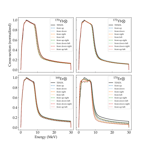
Figure 4: Local predictions from data set $\mathcal{A}$. The solid black line is the TENDL cross section evaluation and each colored dashed line is the prediction from a direct neighbor. The directions’ color-coding and mean absolute error are given in each legend. In this example, all shown cross sections were excluded from the training data (marked with $\otimes$), and some (but not all) neighbors were included.

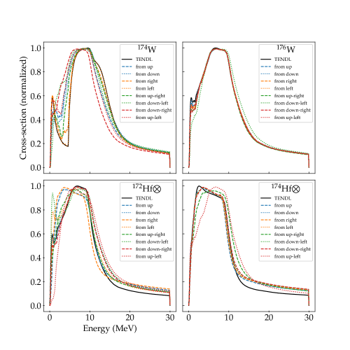
Figure 5: Local predictions from data set $\mathcal{A}$. The solid black line is the TENDL cross section evaluation, and each colored dashed line is the prediction from a direct neighbor. The directions’ color-coding and mean absolute error are given in each legend. In this example, the bottom two cross sections were excluded from the training data (marked with $\otimes$), as were several others below those.

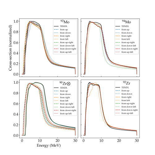
Figure 6: Local predictions from data set $\mathcal{B}$. The solid black line is the TENDL cross section evaluation, and each colored dashed line is the prediction from a direct neighbor. The directions’ color-coding and mean absolute error are given in each legend. In this example, the ⁹⁰Zr cross section was excluded from the training data (marked with $\otimes$).

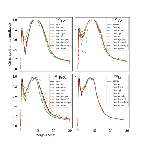
Figure 7: Local predictions from data set $\mathcal{B}$. The solid black line is the TENDL cross section evaluation, and each colored dashed line is the prediction from a direct neighbor. The directions’ color-coding and mean absolute error are given in each legend. The ¹⁵⁸Er cross section was excluded from the training data (marked with $\otimes$) in this example.

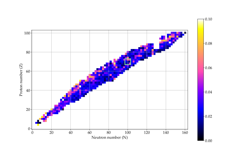
Figure 8: Average error from immediate neighbors, trained on data without 3x3 region around ¹⁷⁰Yb (outlined in green).

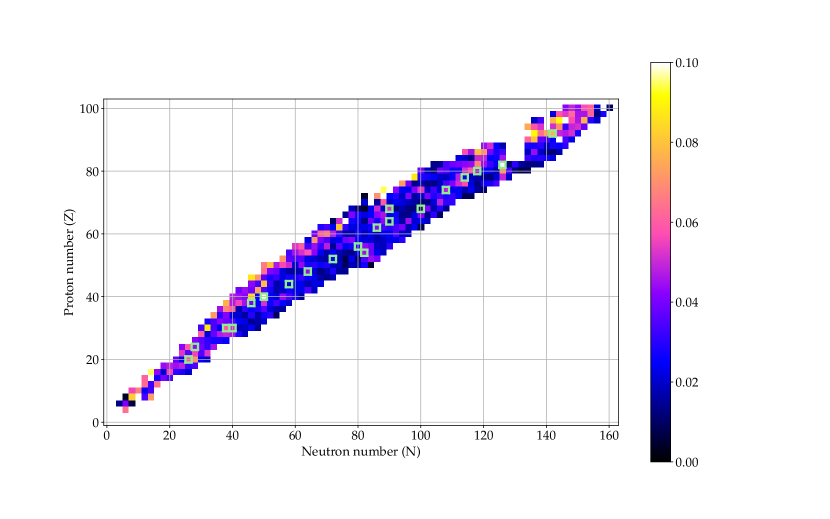
Figure 9: Average error from immediate neighbors, trained on data without a scattered subset of 20 nuclides (outlined in green). This model had been trained for far less time than that shown in Fig. 8, hence the larger errors for some nuclei.

IV.1 Transformation convolutions

Since each generator learns changes in cross sections according to a particular physical change in $N$ and $Z$, we can make predictions in stepwise paths across the chart by convolving transformations. This process is not restricted to the region of training data. The accuracy and stability of predictions appear to be dependent on the complexity of local trends around where the predictions are made. Each chain of predictions is stable for a number of steps, empirically around 5-6 on average, but can be longer or shorter depending on trends locally present and the introduction of drastically anomalous data. Some examples of interpolation are given in Figs. 10, 11, 12, and 13. These examples show a list of TENDL cross sections in one plot and a list of extrapolated GAN predictions in the other.

The first predicted curve $\sigma^{\prime}_{(N,Z)}$ is simply the first cross section $\sigma_{(N,Z)}$ encoded and decoded once, as in

$$\sigma^{\prime}_{(N,Z)}=E^{+}(E(\sigma_{(N,Z)}))=E^{+}(\tilde{z}^{\prime}_{(N+2,Z+2)}).$$ (12)

The second, $\sigma^{\prime}_{(N,Z)+d}$, is the first cross section encoded, transformed once, and decoded, as in

$$\sigma^{\prime}_{(N,Z)+d}=E^{+}(T_{d}(E(\sigma_{(N,Z)})))=E^{+}(\tilde{z}^{\prime}_{(N,Z)+d}))),$$ (13)

where $d$ is the direction of transformation. The third, $\sigma^{\prime}_{(N,Z)+2d}$, is the first cross section encoded, transformed twice, and decoded, as in

$$\sigma^{\prime}_{(N,Z)+2d}=E^{+}(T_{d}(T_{d}(E(\sigma_{(N,Z)}))))=E^{+}(\tilde{z}^{\prime}_{(N,Z)+2d}))).$$ (14)

This may be repeated for $n$ steps: $\sigma^{\prime}_{(N,Z)+nd}=E^{+}(T^{n}_{d}(E(\sigma_{(N,Z)})))$.

Furthermore, transformations in the convolution need not be restricted to one file; relaxing this constraint leads to the ensemble capabilities discussed in the next section. Consider a convolution of the form

$$\sigma^{\prime}_{(N^{\prime},Z^{\prime})}=E^{+}\left(\prod_{d\in\mathcal{D}}T_{d}(E(\sigma_{(N,Z)})\right),$$ (15)

where $\mathcal{D}$ is a sequence of directions. This convolution is tantamount to moving along a path on the chart of nuclides, beginning at $(N,Z)$, following steps in the sequence $\mathcal{D}$, and terminating at $(N^{\prime},Z^{\prime})$.

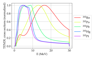
(a) TENDL cross sections

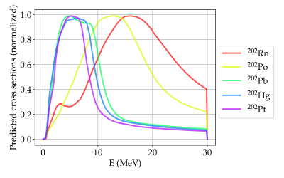
(b) GAN predictions

Figure 10: Cross sections in the $(N,Z)\rightarrow(N+2,Z-2)$ direction ($\searrow$), beginning at ²⁰²Rn for 5 steps. In this case, the GAN reproduces the larger trends well, and only smaller features are lost by the end of the interpolation (purple curve).

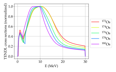
(a) TENDL cross sections

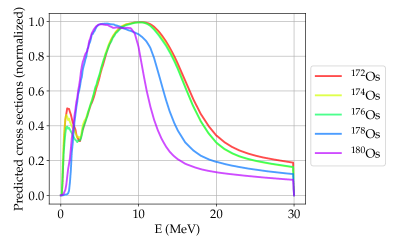
(b) GAN predictions

Figure 11: Cross sections in the $(N,Z)\rightarrow(N+2,Z)$ direction ($\rightarrow$), beginning at ¹⁷²Os for 5 steps. The GAN makes good predictions for the first three steps but changes at ¹⁷⁸Os, beyond which it no longer reproduces the low-energy structure or long tail.

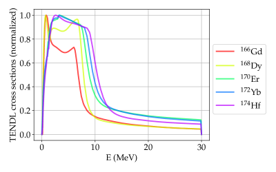
(a) TENDL cross sections

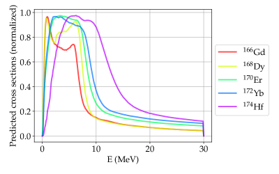
(b) GAN predictions

Figure 12: Cross sections in the $(N,Z)\rightarrow(N,Z+2)$ direction ($\uparrow$), beginning at ¹⁶⁶Gd for 5 steps. This sequence is reproduced nicely by the model until the fifth step to ¹⁷⁴Hf, which shows noticeable errors.

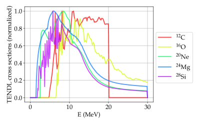
(a) TENDL cross sections

(b) GAN predictions

Figure 13: Cross sections in the $(N,Z)\rightarrow(N+2,Z+2)$ direction ($\nearrow$), beginning at ¹²C for 5 steps. Here we see the GAN reconstructing the ¹²C curve (red) very accurately, but beyond that, the predictions show significant errors. These inaccuracies are due to the fine-tuning of cross section data for this region of the chart (note the high-frequency fluctuations), but also, the trends present in $Z_{\neswarrow}$ are arguably more complex than other subsets (due to changes in both $Z$ and $A$). In that sense, these predictions are the most challenging, and the large inaccuracy shown here is expected.

IV.2 Ensemble predictions

Leveraging the prediction capability, we can perform ensemble predictions for cross sections beyond the training set as well. Ensemble methods can be used in many different machine learning problems and are useful because the model(s) produce a set of predictions rather than just one, and thus we have a built-in measure of variability. In our GAN, this consists of computing many paths across the chart and predicting the cross section at a common final nuclide using the full set of transforms.

Neural network models are commonly understood to have difficulty with extrapolations, at least without the proper modifications. Regularization, which is basically an additional constraint, can help us produce better extrapolations. In particular, distribution learning and constraints placed on latent space distributions of data can be helpful. The VAE, for instance, limits the distribution of latent variables using variational Bayes, and this results in a fantastically smooth latent representation (see [29] for more). Our working hypothesis is that distribution learning may be leveraged to achieve good extrapolation behavior; this certainly helps achieve good results within this work, but proof of this concept does not, to our knowledge, exist.

Ensemble predictions are formed by a set of individual prediction chains. We first designate a target nuclide and a region of the chart for the starting points. Then, we compute all possible paths which begin within our region of interest and terminate on the target. An added constraint is that the paths do not “back-track”; that is, within each path, the distance to the target nuclide is monotonically decreasing with each step. This property ensures that we are not including undue errors in the ensemble. In this way, the calculation in Eq. 15 is done for many different paths $\mathcal{D}$, which constitute a sampling of $P(\sigma^{\prime}|\mathcal{D})$, the distribution of ensemble predictions.

Examples of ensemble predictions are shown in Figures 14, 15, 16, 17, and 18. Each figure shows the TENDL cross section evaluation in pink and the predicted ensemble in thin, colored lines. In the upper (a) plots, the line color corresponds to the number of steps in the path leading to that prediction (see color bar). In lower (b) plots, we show the results of a Gaussian weighted average with predictions weighted by the inverse square of the path length (in the number of steps), so predictions with more linked model evaluations are discounted. This model-averaging technique is by no means rigorous and is included here primarily to aid visual interpretation. Figures 14 and 15 show good predictions and a reasonable spread of errors. As can be seen in Fig. 15, short paths are generally more accurate than long paths. This makes sense since predictions from longer paths might accumulate errors that compound with each application.

Fig. 16 shows predictions for Cerium-158, which does not have a cross section evaluation in the TENDL library. Interestingly, we see the ensemble prediction is bimodal; that is, each prediction is centered around one of two curves. The first mode increases very fast at 0 MeV, then has a shorter secondary peak around 6 MeV (which is a very common feature in the inelastic neutron scattering channel). It corresponds to predictions from shorter paths (blue and green curves), so it is likely more accurate. The second mode, which only has one major peak around 5 MeV, is created by longer paths (yellow and red curves) and thus is likely not as accurate as the other. We can thus inspect the ensemble result and glean a prediction for the cross section of Cerium-158, which does not have experimental measurements. The confidence band is estimated according to the spread in the ensemble.

Lastly, Fig. 18 illustrates an ensemble prediction with large variability. Ensemble predictions for heavy nuclides, like Uranium-234, are likely not as accurate as those for lighter nuclides, partly because there are fewer data points for heavy nuclides in the training data (which can be seen as the chart gets thinner at the heavy end, nuclides have fewer around them). Furthermore, the ²³⁸U cross section evaluation has been carefully tuned and thus may break from global systematic trends learned by the GAN. A future priority for this research may be to decide how to better summarize these ensemble predictions with large variance.

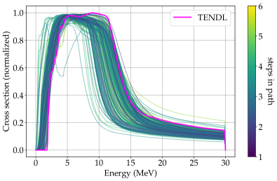
(a) Ensemble prediction of ⁸⁸Sr with all 273 predicted curves shown. GAN predictions are shown in viridis (blue-green-yellow) where the color corresponds to the number of transform applications (i.e. length of path across chart).

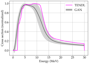
(b) Ensemble prediction of ⁸⁸Sr represented by a median and standard deviation band, which is computed using a weighted average of curves in the ensemble.

Figure 14: Ensemble prediction of the (normalized) cross section of Strontium-88, using all possible paths within a bounded local region of the chart of nuclides. Almost all curves in our ensemble are reasonable in shape, but many show the reaction turning off at lower energies than observed.

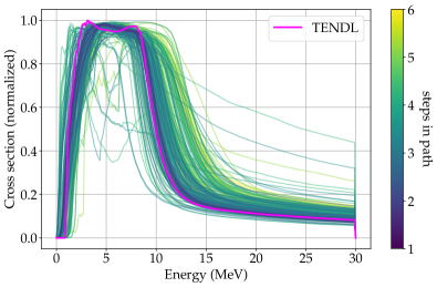
(a) Ensemble prediction of ⁹⁴Zr with all 260 predicted curves shown. GAN predictions are shown in viridis (blue-green-yellow) where the color corresponds to the number of transform applications (i.e. length of path across chart).

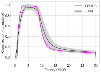
(b) Ensemble prediction of ⁹⁴Zr represented by a median and standard deviation band, which is computed using a weighted average of curves in the ensemble.

Figure 15: Ensemble prediction of the (normalized) cross section of Zirconium-94, using all possible paths within a bounded local region of the chart of nuclides. This example is included to illustrate the benefit of averaging over the ensemble: some individual predictions have large errors but the ensemble median predicts the cross section well.

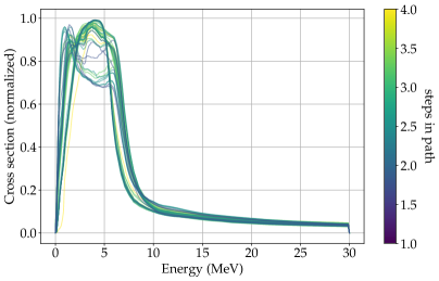
(a) Ensemble prediction of ¹⁵⁸Ce with all 57 predicted curves shown. GAN predictions are shown in viridis (blue-green-yellow) where the color corresponds to the number of transform applications (i.e. length of path across chart).

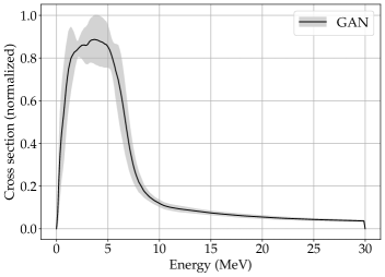
(b) Ensemble prediction of ¹⁵⁸Ce represented by a median and standard deviation band, which is computed using a weighted average of curves in the ensemble.

Figure 16: Ensemble prediction of the (normalized) cross section of Cerium-158, using all possible paths within a bounded local region of the chart of nuclides. TENDL does not include an evaluation for this cross section, so this prediction may be considered an extrapolation.

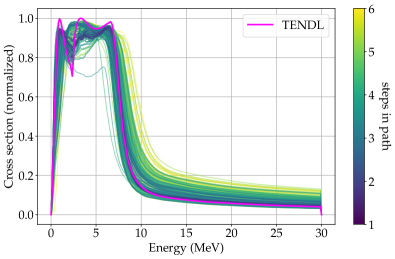
(a) Ensemble prediction of ¹⁵⁸Sm with all 213 predicted curves shown. GAN predictions are shown in viridis (blue-green-yellow) where the color corresponds to the number of transform applications (i.e. length of path across chart).

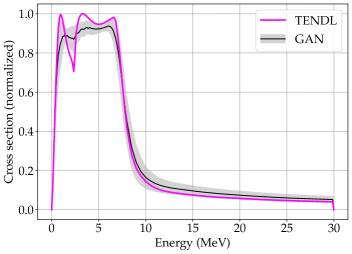
(b) Ensemble prediction of ¹⁵⁸Sm represented by a median and standard deviation band, which is computed using a weighted average of curves in the ensemble.

Figure 17: Ensemble prediction of the (normalized) cross section of Samarium-158, using all possible paths within a bounded local region of the chart of nuclides. While the ensemble reproduces the curve with small errors, the strong resonance around 2 MeV is only predicted by fewer than half of the ensemble curves.

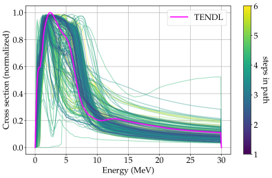
(a) Ensemble prediction of ²³⁴U with all 272 predicted curves shown. GAN predictions are shown in viridis (blue-green-yellow) where the color corresponds to the number of transform applications (i.e. length of path across chart).

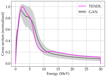
(b) Ensemble prediction of ²³⁴U represented by a median and standard deviation band, which is computed using a weighted average of curves in the ensemble.

Figure 18: Ensemble prediction of the (normalized) cross section of Uranium-234, using all possible paths within a bounded local region of the chart of nuclides. Larger errors are expected for very heavy (and very light) nuclides, and significant variability can be seen in the individual predictions. Averaging, however, shows the true cross section indeed lies within the confidence band.

V Conclusion

We have developed a deep generative machine learning model to learn intricate systematic trends in nuclear cross section evaluations in a subset of the TENDL library. The model uses well-established machine learning models, namely the variational autoencoder and generative adversarial network, but we have made several important modifications to these models to suit the problem of nuclear data, and thus, it is a novel development. The model is capable of accurately predicting cross sections as particle pairs are added and subtracted from the target nucleus, at least within local regions on the chart of nuclides.

This can be used for interpolations and extrapolations, chaining together of predictions, and producing an ensemble of predictions for cross section evaluations. Ensemble predictions are very powerful as they can naturally be used to predict cross sections outside the library and estimate confidence intervals. However, how exactly the ensemble of curves should be transformed into a single estimate of the cross section is nontrivial, and the solution (possibly Bayesian model-mixing [30]) is beyond the scope of this paper.

Although the present model is perhaps not well suited for scaling to larger problems, such as leveraging important correlations between reaction channels, we hope this research can inspire other researchers to bring creativity and insight to this problem.

VI Acknowledgments

This work was performed under the auspices of the U.S. Department of Energy by Lawrence Livermore National Laboratory under Contract DE-AC52-07NA27344, supported in part through the Laboratory Directed Research and Development under project 23-SI-004. JF is supported by the U.S. Department of Energy, Office of Science, Office of Nuclear Physics contract DE-AC02-06CH11357, as well as the SCGSR program, the NUCLEI SciDAC program, and Argonne LDRD awards. Computing support came in part from the LLNL institutional Computing Grand Challenge program.

Appendix A Simple GANs

Generative models are a family of machine learning techniques designed to learn a probability distribution. The VAE discussed in the last section is a generative model: the decoder network can be fed a normal random variable and generate random samples of the target distribution. What sets the GAN apart is a modification of the generator network’s loss function: rather than relying on the latent space distribution of data, one introduces an entirely separate network to identify definitive trends in training data and penalizes the generating network when the output does not match those trends. As such, the adversarial nature of the model allows for a generalization of the statistical requirements we had in the VAE.

The simplest GANs consist of two networks: one generator $G$ and one discriminator $D$, both acting on data $x\in X$. The generator learns a mapping from a standard normal to the target distribution, and the discriminator scores the validity of generated data, $D(x^{\prime})=P(x^{\prime}\in X|x\in X)$. This type of GAN is useful for fully unsupervised learning; that is, the generator learns the relevant probability distribution without any labeled inputs (aside from the labels for $x\in X$ and $G(x)\not\in X$, which are supplied to the discriminator, but these are trivial to generate).

During training, the weights of networks $G$ and $D$ are optimized with respect to a loss function, and the networks compete with one another in what is notoriously tantamount to finding a Nash equilibrium. Methods for reliable GAN training is an open area of research. Training the system results in a generator that can “convincingly” (according to the discriminator) create new samples $x^{\prime}$, the correlations of which closely resemble those of the training data. We introduce the notation $x^{\prime}\;\tilde{\in}\;X$, meaning $x^{\prime}$ closely resembles an element of the set $X$, or similarly $x^{\prime}$ looks like a sample of the distribution from which $X$ could be drawn, $x^{\prime}\sim P(X)$. We denote this simple GAN as the pair $\{G,D\}$. We can write the networks as explicit functions of weights $\theta$ as $G=G(\theta_{G})$ and $D=D(\theta_{D})$ for clarity.

The loss function for the simple GAN is different for the generator and discriminator, but both can be expressed in terms of the following two expectation values ($\mathbb{E}$).

$$v=\mathbb{E}_{x\sim P(X)}\log(D(x))+\mathbb{E}_{x\sim P(G)}\log(1-D(x))$$ (16)

The distribution $P(G)$ means the distribution of the generator samples. The respective loss functions are $\mathcal{L}_{G}(\theta_{G})=v(\theta_{G})$ and $\mathcal{L}_{D}(\theta_{D})=-v(\theta_{D})$. The discriminator loss is low when it correctly identifies both true data and generated data, thus both terms are large. The generator loss only depends on the second term and is low when the discriminator assigns a high probability to the generator outputs; thus, we might say the discriminator is being “deceived”, classifying the generated data as real.

Although finding a true Nash equilibrium is ideal, this can be very difficult in practice. If both networks are training, that which has the advantage will fluctuate, but this process can continue for a long time without a clear indication of making progress. An approximation may be found by first training a discriminator to effectively classify the data, then subsequently training the generator by itself. So, it is common for GANs to be trained this way, repeating the process to produce a better approximation to equilibrium.

In practice, we may express this loss function in Eq. 16 in a slightly different way. One often uses a loss function like binary cross-entropy (BCE) to evaluate probabilities, which the discriminator network emits. BCE is the preferred loss function when the classifier network ends with a single sigmoid neuron: it compares a label probability $y$ with a predicted probability $p$ and produces one number that decreases as $y\rightarrow p$. (In practice, one may design a classifier that emits a so-called logit value on $(-\infty,+\infty)$ and a modified version of the BCE to handle logits instead of probabilities. This is mathematically equivalent but might allow for better convergence in some cases.)

$$BCE\left[p,y\right]:=-\left[y\log(p)+(1-y)\log(1-p)\right]$$ (17)

BCE can also be evaluated for a set of inputs, as in batch training, simply by averaging the individual BCE values for each pair. In terms of BCE for a single batch of $N_{b}$ data points, the adversarial loss function is the sum of $\mathcal{L}_{D}$ and $\mathcal{L}_{G}$ in Eq. 18.

$$\mathcal{L}_{D}(\theta_{D}) =\frac{1}{N_{b}}\sum_{i=1}^{N_{b}}\left[BCE[D(x_{i}),1]+BCE[D(G(z_{i})),0]\right]$$ (18)

$$\mathcal{L}_{G}(\theta_{G}) =\frac{1}{N_{b}}\sum_{i=1}^{N_{b}}BCE[D(G(z_{i})),1]$$

Ultimately, the GAN learns to approximate the probability distribution of the data $P(X)$, and the evaluation of the generator on random noise $G(z)$ approximates sampling from $P(X)$. To better adapt the model to our nuclear data problem, we consider a slightly more advanced form called the cycle-consistent GAN.

Appendix B Challenges with the convolutional GAN

Our initial attempts at this project involved not the separate convolutional VAE and dense GAN but rather a single convolutional GAN, which was intended to learn both latent space encodings and transforms of cross sections. This construction was difficult to work with, and although it is not clear why, we may learn some things by comparing that model to this final version. In the old model, the generator of the cycleGAN followed a U-net design [31], which is very successful when applied to image datasets. The U-net design has shown success in GAN models on 2D image data, so our assumption was that 1D cross section data is similar enough that we could use a 1D version of the same model structure. The loss function was the same as that of our dense GAN; the discriminator network followed the design of a simple multi-layer convolutional classifier. However, when training it, we found the U-net model to have poor convergence properties. It was especially difficult to control overfitting while maintaining good predictions and optimizing the coefficient of target loss. If the coefficient $\lambda_{\text{target}}$ is too large, then the model would overfit, and predictions would be unreliable; if it were too small, the model would not converge (i.e., predicted cross sections were very noisy and would not match the training set).

An interesting physics connection can be seen in comparing the results of the U-net with the one presented. Since the U-net would not converge fully, it could not learn systematic trends across the chart, and in particular, Fig. 19 shows that error increases around $N=50$ and 82, which are magic numbers. This indicates that the model had not learned to incorporate changes in the cross sections that are due to shell structure; such errors are not present in the final version of our model.

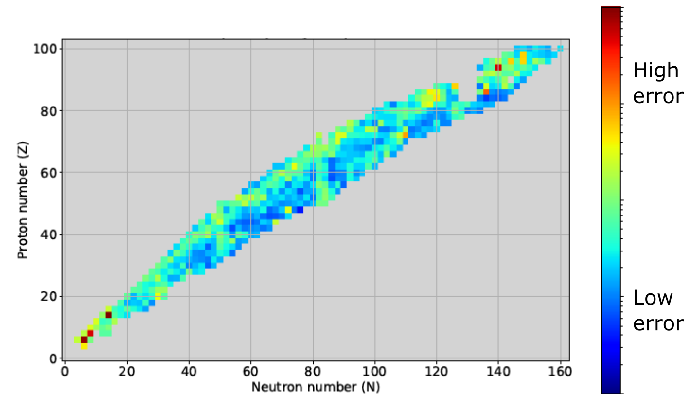
Figure 19: Average error of local predictions using the U-net GAN model, which was prone to overfitting, unstable, and ultimately abandoned in favor of the VAE+GAN system. Note that higher errors are clearly visible around magic numbers $N=50,82$, indicating the model has not learned how cross sections are dependent on shell structure. The nuclides with very high error (red) are those where the cross-section is far more detailed than its neighbors (e.g., O¹⁶).

This is not to say that a 1D U-net style cycleGAN is a poor design in general, only that in our particular implementation for this problem, it did not give good results. Whether that model could be successful in some nuclear data applications may be a worthy question to pursue, but that is beyond the scope of this research.

References

- Weizsacker [1935] C. F. V. Weizsacker, Zur Theorie der Kernmassen, Z. Phys. 96, 431 (1935).
- Hagen et al. [2015] G. Hagen et al., Neutron and weak-charge distributions of the 48Ca nucleus, Nature Phys. 12, 186 (2015), arXiv:1509.07169 [nucl-th] .
- Fattoyev et al. [2018] F. J. Fattoyev, J. Piekarewicz, and C. J. Horowitz, Neutron skins and neutron stars in the multimessenger era, Phys. Rev. Lett. 120, 172702 (2018).
- Brown et al. [2018] D. Brown, M. Chadwick, R. Capote, A. Kahler, A. Trkov, M. Herman, A. Sonzogni, Y. Danon, A. Carlson, M. Dunn, D. Smith, G. Hale, G. Arbanas, R. Arcilla, C. Bates, B. Beck, B. Becker, F. Brown, R. Casperson, J. Conlin, D. Cullen, M.-A. Descalle, R. Firestone, T. Gaines, K. Guber, A. Hawari, J. Holmes, T. Johnson, T. Kawano, B. Kiedrowski, A. Koning, S. Kopecky, L. Leal, J. Lestone, C. Lubitz, J. Márquez Damián, C. Mattoon, E. McCutchan, S. Mughabghab, P. Navratil, D. Neudecker, G. Nobre, G. Noguere, M. Paris, M. Pigni, A. Plompen, B. Pritychenko, V. Pronyaev, D. Roubtsov, D. Rochman, P. Romano, P. Schillebeeckx, S. Simakov, M. Sin, I. Sirakov, B. Sleaford, V. Sobes, E. Soukhovitskii, I. Stetcu, P. Talou, I. Thompson, S. van der Marck, L. Welser-Sherrill, D. Wiarda, M. White, J. Wormald, R. Wright, M. Zerkle, G. Žerovnik, and Y. Zhu, Endf/b-viii.0: The 8th major release of the nuclear reaction data library with cielo-project cross sections, new standards and thermal scattering data, Nuclear Data Sheets 148, 1 (2018), special Issue on Nuclear Reaction Data.
- Plompen, A. J. M. et al. [2020] Plompen, A. J. M., Cabellos, O., De Saint Jean, C., Fleming, M., Algora, A., Angelone, M., Archier, P., Bauge, E., Bersillon, O., Blokhin, A., Cantargi, F., Chebboubi, A., Diez, C., Duarte, H., Dupont, E., Dyrda, J., Erasmus, B., Fiorito, L., Fischer, U., Flammini, D., Foligno, D., Gilbert, M. R., Granada, J. R., Haeck, W., Hambsch, F.-J., Helgesson, P., Hilaire, S., Hill, I., Hursin, M., Ichou, R., Jacqmin, R., Jansky, B., Jouanne, C., Kellett, M. A., Kim, D. H., Kim, H. I., Kodeli, I., Koning, A. J., Konobeyev, A. Yu., Kopecky, S., Kos, B., Krása, A., Leal, L. C., Leclaire, N., Leconte, P., Lee, Y. O., Leeb, H., Litaize, O., Majerle, M., Márquez Damián, J. I, Michel-Sendis, F., Mills, R. W., Morillon, B., Noguère, G., Pecchia, M., Pelloni, S., Pereslavtsev, P., Perry, R. J., Rochman, D., Röhrmoser, A., Romain, P., Romojaro, P., Roubtsov, D., Sauvan, P., Schillebeeckx, P., Schmidt, K. H., Serot, O., Simakov, S., Sirakov, I., Sjöstrand, H., Stankovskiy, A., Sublet, J. C., Tamagno, P., Trkov, A., van der Marck, S., Álvarez-Velarde, F., Villari, R., Ware, T. C., Yokoyama, K., and Žerovnik, G., The joint evaluated fission and fusion nuclear data library, jeff-3.3, Eur. Phys. J. A 56, 181 (2020).
- Koning et al. [2019] A. Koning, D. Rochman, J.-C. Sublet, N. Dzysiuk, M. Fleming, and S. van der Marck, Tendl: Complete nuclear data library for innovative nuclear science and technology, Nuclear Data Sheets 155, 1 (2019), special Issue on Nuclear Reaction Data.
- Feng and Zalutsky [2021] Y. Feng and M. R. Zalutsky, Production, purification and availability of 211at: Near term steps towards global access, Nuclear Medicine and Biology 100-101, 12 (2021).
- Bedaque et al. [2021] P. Bedaque, A. Boehnlein, M. Cromaz, M. Diefenthaler, L. Elouadrhiri, T. Horn, M. Kuchera, D. Lawrence, D. Lee, S. Lidia, et al., Ai for nuclear physics, The European Physical Journal A 57, 1 (2021).
- Boehnlein et al. [2022] A. Boehnlein, M. Diefenthaler, N. Sato, M. Schram, V. Ziegler, C. Fanelli, M. Hjorth-Jensen, T. Horn, M. P. Kuchera, D. Lee, W. Nazarewicz, P. Ostroumov, K. Orginos, A. Poon, X.-N. Wang, A. Scheinker, M. S. Smith, and L.-G. Pang, Colloquium: Machine learning in nuclear physics, Reviews of Modern Physics 94, 031003 (2022).
- He et al. [2023a] W.-B. He, Y.-G. Ma, L.-G. Pang, H. Song, and K. Zhou, High energy nuclear physics meets machine learning 10.48550/arXiv.2303.06752 (2023a), arXiv:2303.06752 [hep-ex, physics:hep-ph, physics:nucl-ex, physics:nucl-th].
- He et al. [2023b] W. He, Q. Li, Y. Ma, Z. Niu, J. Pei, and Y. Zhang, Machine learning in nuclear physics at low and intermediate energies 10.48550/arXiv.2301.06396 (2023b), arXiv:2301.06396 [nucl-ex, physics:nucl-th].
- Gao et al. [2021] Z.-P. Gao, Y.-J. Wang, H.-L. Lü, Q.-F. Li, C.-W. Shen, and L. Liu, Machine learning the nuclear mass, Nuclear Science and Techniques 32, 109 (2021).
- Mumpower et al. [2022] M. R. Mumpower, T. M. Sprouse, A. E. Lovell, and A. T. Mohan, Physically interpretable machine learning for nuclear masses, Physical Review C 106, 10.1103/physrevc.106.l021301 (2022).
- Niu and Liang [2022] Z. M. Niu and H. Z. Liang, Nuclear mass predictions with machine learning reaching the accuracy required by -process studies, Physical Review C 106, L021303 (2022).
- Grechanuk et al. [2021] P. A. Grechanuk, M. E. Rising, and T. S. Palmer, Application of machine learning algorithms to identify problematic nuclear data, Nuclear Science and Engineering 195, 1265–1278 (2021).
- Adams et al. [2021] C. Adams, G. Carleo, A. Lovato, and N. Rocco, Variational monte carlo calculations of nuclei with an artificial neural-network correlator ansatz, Physical Review Letters 127, 022502 (2021).
- Rigo et al. [2023] M. Rigo, B. Hall, M. Hjorth-Jensen, A. Lovato, and F. Pederiva, Solving the nuclear pairing model with neural network quantum states, Physical Review E 107, 025310 (2023).
- Lovato et al. [2022] A. Lovato, C. Adams, G. Carleo, and N. Rocco, Hidden-nucleons neural-network quantum states for the nuclear many-body problem, Physical Review Research 4, 043178 (2022).
- Goodfellow et al. [2014] I. J. Goodfellow, J. Pouget-Abadie, M. Mirza, B. Xu, D. Warde-Farley, S. Ozair, A. Courville, and Y. Bengio, Generative Adversarial Networks, arXiv e-prints , arXiv:1406.2661 (2014), arXiv:1406.2661 [stat.ML] .
- Karras et al. [2018] T. Karras, S. Laine, and T. Aila, A Style-Based Generator Architecture for Generative Adversarial Networks, arXiv e-prints , arXiv:1812.04948 (2018), arXiv:1812.04948 [cs.NE] .
- Radford et al. [2015] A. Radford, L. Metz, and S. Chintala, Unsupervised Representation Learning with Deep Convolutional Generative Adversarial Networks, arXiv e-prints , arXiv:1511.06434 (2015), arXiv:1511.06434 [cs.LG] .
- Gonzalez-Garcia et al. [2018] A. Gonzalez-Garcia, J. van de Weijer, and Y. Bengio, Image-to-image translation for cross-domain disentanglement, arXiv e-prints , arXiv:1805.09730 (2018), arXiv:1805.09730 [cs.CV] .
- Huang et al. [2018] X. Huang, M.-Y. Liu, S. Belongie, and J. Kautz, Multimodal Unsupervised Image-to-Image Translation, arXiv e-prints , arXiv:1804.04732 (2018), arXiv:1804.04732 [cs.CV] .
- Zhu et al. [2017a] J.-Y. Zhu, R. Zhang, D. Pathak, T. Darrell, A. A. Efros, O. Wang, and E. Shechtman, Toward Multimodal Image-to-Image Translation, arXiv e-prints , arXiv:1711.11586 (2017a), arXiv:1711.11586 [cs.CV] .
- Zhu et al. [2017b] J.-Y. Zhu, T. Park, P. Isola, and A. A. Efros, Unpaired Image-to-Image Translation using Cycle-Consistent Adversarial Networks, arXiv e-prints , arXiv:1703.10593 (2017b), arXiv:1703.10593 [cs.CV] .
- Rajput et al. [2021] P. S. Rajput, K. Satis, S. Dellarosa, W. Huang, and O. Agba, cgans for cartoon to real-life images (2021).
- Kingma and Ba [2014] D. P. Kingma and J. Ba, Adam: A Method for Stochastic Optimization, arXiv e-prints , arXiv:1412.6980 (2014), arXiv:1412.6980 [cs.LG] .
- Yazıcı et al. [2018] Y. Yazıcı, C.-S. Foo, S. Winkler, K.-H. Yap, G. Piliouras, and V. Chandrasekhar, The Unusual Effectiveness of Averaging in GAN Training, arXiv e-prints , arXiv:1806.04498 (2018), arXiv:1806.04498 [stat.ML] .
- Kingma and Welling [2013] D. P. Kingma and M. Welling, Auto-encoding variational bayes, arXiv preprint arXiv:1312.6114 (2013).
- Hoeting et al. [1999] J. A. Hoeting, D. Madigan, A. E. Raftery, and C. T. Volinsky, Bayesian model averaging: a tutorial (with comments by M. Clyde, David Draper and E. I. George, and a rejoinder by the authors, Statistical Science 14, 382 (1999).
- Ronneberger et al. [2015] O. Ronneberger, P. Fischer, and T. Brox, U-Net: Convolutional Networks for Biomedical Image Segmentation, arXiv e-prints , arXiv:1505.04597 (2015), arXiv:1505.04597 [cs.CV] .