Uniform-over-dimension convergence with application to location tests for high-dimensional data
Abstract
Asymptotic methods for hypothesis testing in high-dimensional data usually require the dimension of the observations to increase to infinity, often with an additional condition on its rate of increase compared to the sample size. On the other hand, multivariate asymptotic methods are valid for fixed dimension only, and their practical implementations in hypothesis testing methodology typically require the sample size to be large compared to the dimension for yielding desirable results. However, in practical scenarios, it is usually not possible to determine whether the dimension of the data at hand conform to the conditions required for the validity of the high-dimensional asymptotic methods, or whether the sample size is large enough compared to the dimension of the data. In this work, a theory of asymptotic convergence is proposed, which holds uniformly over the dimension of the random vectors. This theory attempts to unify the asymptotic results for fixed-dimensional multivariate data and high-dimensional data, and accounts for the effect of the dimension of the data on the performance of the hypothesis testing procedures. The methodology developed based on this asymptotic theory can be applied to data of any dimension. An application of this theory is demonstrated in the two-sample test for the equality of locations. The test statistic proposed is unscaled by the sample covariance, similar to usual tests for high-dimensional data. Using simulated examples, it is demonstrated that the proposed test exhibits better performance compared to several popular tests in the literature for high-dimensional data. Further, it is demonstrated in simulated models that the proposed unscaled test performs better than the usual scaled two-sample tests for multivariate data, including the Hotelling’s test for multivariate Gaussian data.
keywords:
[class=MSC]keywords:
corollarytheorem \aliascntresetthecorollary \newaliascntlemmatheorem \aliascntresetthelemma \newaliascntpropositiontheorem \aliascntresettheproposition \newaliascntdefinitiontheorem \aliascntresetthedefinition \newaliascntremarktheorem \aliascntresettheremark \endlocaldefs
, and
1 Introduction
In diverse studies and scientific experiments, observations generated are high-dimensional in nature, i.e., the dimension of the observation vectors are higher than the number of observations (see, e.g., [8, 26, 19, 6]). There is an extensive literature on high-dimensional one-sample and multi-sample tests of means, or more generally, of the locations/centers of the underlying distributions ([16, 12, 24, 5, 7, 25, 18, 9]). In many asymptotic results involving high-dimensional data, authors make the assumption that the dimension along with sample size (see, e.g., [2, 12, 27]). In many other results, there are conditions on the rate of growth of , e.g., for some (see, e.g., [17]). However, these conditions on the dimension are not easy to verify, and it is often unclear whether they are satisfied in a particular situation or not. In a practical situation of testing, an experimenter has only one sample of observations, which fixes the value of and . Based on just this one pair of and , it is not possible to verify whether satisfies the particular rate with respect to required for the validity of those aforementioned results.
Multivariate asymptotic results for an extensive collection of statistics are well-established in the literature. These results are based on the assumption of a fixed value of and taking to infinity. However, in practice, except when is very small compared to , sometimes it is observed that existing asymptotic results provide unsatisfactory approximations to the actual distributions of the test statistics for moderate values of , which are still far lower compared to .
In this work, we develop an asymptotic theory of convergence which holds uniformly over the dimension . This eliminates the concern over the validity of the asymptotic conditions on the dimension, which are generally found in existing results. The asymptotic results developed using this theory can be applied to data with arbitrary dimensions, including usual multivariate as well as high-dimensional data.
Suppose one carries out a test of hypothesis based on independent -dimensional observations . The test statistic in any such hypothesis test, is always univariate, whatever the value of the dimension of the data might be. This observation motivates the setup we consider for developing the uniform-over-dimension asymptotic theory of convergence. We define uniform-over-dimension convergence in distribution of functions of random vectors and state its associated results, which are analogous to the usual results for convergence in distribution. More specifically, we consider functions of -dimensional random vectors , where and is some positive integer, and define the uniform-over- convergence of . For a test statistic, is 1, but we consider general integer values of while developing the theory, which helps in deriving subsequent results. Often, a test statistic can be decomposed in two components, one of which is asymptotically negligible, and it is easier to derive the asymptotic distribution of the other component. To implement similar techniques in deriving uniform-over-dimension asymptotic distributions, we define uniform-over-dimension convergence in probability of functions of random vectors, and state associated results concerning both uniform-over-dimension convergence in distribution and convergence in probability.
The proposed theory is demonstrated on a test for equality of locations and deriving the uniform-over-dimension asymptotic null distribution of the test statistic. The proposed test statistic is constructed based on a kernel, without using normalization by the sample covariance matrix. Normalization by the sample covariance is not usually used for high-dimensional tests, and we have followed a similar principle here. However, we propose the test to be applied without regard to the dimension of the data, whether high-dimensional or standard multivariate situations. A natural question arises about the performance of the proposed testing method without normalization in case of multivariate data, where normalization by sample covariance is usually employed. However, we have shown using simulated as well as real data analyses that the proposed test outperforms the other tests, both in high-dimensional and lower-dimensional multivariate data, in Gaussian as well as non-Gaussian models.
In section 2, the definitions and theorems related to uniform-over-dimension convergence in distribution and probability of functions of random vectors are presented. In section 3, the proposed theory is employed to derive the asymptotic null distribution of a suggested test of equality of locations of several populations, which is valid uniformly over the dimension of the observations. Further, the asymptotic consistency of the test is also established uniformly over the dimension of the observations. In section 4, it is demonstrated using simulated and real data that the proposed test equipped with its asymptotic null distribution valid uniformly over the data dimension outperforms other tests available for both high-dimensional and usual multivariate data. In section 5, further work on the proposed theory and potential applications are discussed. Proofs of the mathematical results are presented in the Appendix.
2 Main theoretical results
In this section, we define uniform-over-dimension convergence in distribution and in probability, and state the associated results. In the first subsection, the uniform-over-dimension convergence in distribution is defined and its associated results are stated. The uniform-over-dimension convergence in probability is defined in the second subsection, and results involving both the notions of convergence are stated there.
2.1 Definitions and Theorems
Let be -dimensional random vectors with probability measures and associated distribution functions on , where is the Borel sigma field on , and the indices and are positive integers. Also, let be a -dimensional random vector with probability measure and associated distribution function on . We think of as a fixed-dimensional vector-valued function of some -dimensional random vector , and similarly is thought of as a fixed-dimensional vector-valued function of a -dimensional random vector . Although the motivation behind the following theory is the fact that a test statistic is always univariate (i.e., ) irrespective of the dimension of the underlying observations, we are considering vector-valued functions of the observations instead of univariate functions. This consideration turns out to be useful in the proofs of some of the results on uniform-over-dimension convergence of random variables.
Definition \thedefinition.
We say that converges in distribution to uniformly-over- if for every bounded continuous function ,
We write it as either of the following: uniformly-over-, or uniformly-over-, or uniformly-over-.
We proceed to state and prove several results for uniform-over- convergence in distribution, which are analogous to theorems for the usual weak convergence of probability measures (see, e.g., [4]). The following assumption is required for those subsequent results:
-
(A1)
The collection of probability measures on is relatively compact with respect to the total variation metric.
Assumption (A1) means that every sequence in has a subsequence such that as for some probability measure on , where may not be a member of the collection . Now, as implies that as for any -continuity set , i.e., weakly converges to . Since is separable and complete, it follows that is tight (see pp. 57, 59 and Theorem 5.2 in [4]), i.e., given any , there is a compact set such that
| (1) |
Further, from the separability of , it follows that is relatively compact with respect to the metric of weak convergence of probability measures (see point (iv) in page 72 in [4]).
Assumption (A1) implies tightness, which is a common assumption while establishing convergence in distribution for a diverse collection of measures (see, e.g., Theorems 7.1, 7.3, 13.1 and 13.2 in [4]). Although assumption (A1) is stronger than the common assumption of tightness, it is satisfied in diverse cases including those of common interest.
We need the following lemma to prove the uniform-over- analogue of the Portmanteau theorem (cf. Lemma 8.5.1 in [20]).
Lemma \thelemma.
Under assumption (A1), given any Borel set , which is a -continuity set for all , and any , there are bounded and Lipschitz continuous functions such that and , where is the indicator function of the set .
We state the uniform-over- analogue of the Portmanteau theorem (Theorem 2.1 in [4]) below.
Theorem 1 (Uniform-over- Portmanteau theorem).
Let and be as defined above, and assumption (A1) be satisfied. Then, the following are equivalent:
-
(i)
uniformly-over-.
-
(ii)
For every bounded and uniformly continuous function ,
-
(iii)
For every continuous function , which is zero outside of a compact set,
-
(iv)
For every bounded and Lipschitz continuous function ,
-
(v)
For every Borel set , which is a -continuity set for all ,
-
(vi)
For being a continuity point of for all ,
Based on the uniform-over- Portmanteau theorem, we proceed to state the uniform-over- Lévy’s continuity theorem.
Theorem 2 (Uniform-over- Lévy’s continuity theorem).
Let and be probability measures on with characteristic functions and . Then, uniformly-over- if and only if for every , we have
The uniform-over- Lévy’s continuity theorem is the most critical tool to establish the uniform-over- convergence in distribution of a sequence of random variables which are functions of some -variate random vectors. Using this theorem, one needs to only establish that the characteristic functions of those random variables converge uniformly over to establish their uniform-over- convergence in distribution.
The uniform-over- continuous mapping theorem stated below is also a useful result.
Theorem 3 (Uniform-over- continuous mapping theorem).
Let and be -dimensional random vectors with uniformly-over- and be a continuous function. Then, uniformly-over-.
2.2 Uniform-over- Convergence in Probability
In the last section, we studied the asymptotic convergence in distribution of fixed-dimensional random vectors which are functions of possibly high-dimensional random vectors. In this subsection, we concentrate on uniform-over-dimension convergence in probability of fixed-dimensional random vectors which are functions of possibly high-dimensional random vectors.
Definition \thedefinition.
Let and be -dimensional random vectors. We say that uniformly-over- if for every ,
While applying the tools to establish uniform-over-dimension convergence in distribution for a sequence of real-valued random variables, one may come across a corresponding sequence of real-valued random variables such that it is easier to establish the uniform-over-dimension convergence in distribution of the second sequence of random variables and the difference between the two sequences converges to zero in probability uniformly-over-dimension. In such cases, the uniform-over-dimension convergence in distribution for the first sequence can be established using the uniform-over-dimension analogue of Slutsky’s theorem. The following lemma is required to prove the uniform-over- Slutsky’s theorem.
Lemma \thelemma.
Let , and be real-valued random variables and be a bounded sequence of real numbers with uniformly-over- and uniformly-over-. Then, uniformly-over-.
Now, the uniform-over- Slutsky’s theorem follows from Theorem 3 and subsection 2.2.
Theorem 4 (Uniform-over- Slutsky’s theorem).
Let , and be real-valued random variables and be a bounded sequence of real numbers such that uniformly-over- and uniformly-over-. Then,
-
(a)
uniformly-over-,
-
(b)
uniformly-over-,
-
(c)
uniformly-over- if is bounded away from 0, i.e., .
3 Multi-sample location tests
In this section, we demonstrate how the preceding theory of convergence helps us derive asymptotic distributions of test statistics independent of any assumption on the dimension.
Let be a probability measure on , be -dimensional vectors and denote the linear shift of by , i.e., if the random vector has the probability measure , then is the probability measure corresponding to . We consider a sample of size consisting of independent observations generated from the probability measures for . The observations from the measure are denoted as , where and . We are interested in testing the hypothesis
| (2) |
Let satisfy that for all . Define . Also, define . Note that for all under in (2). So, a test of may be conducted based on the magnitudes of for , and a high value of for any would indicate that in (2) is not true. Define the test statistic
The hypothesis in (2) is to be rejected if the value of is large.
When and , we get the test proposed by [27]. We shall denote this test by [27] as ZGZC2020 test in our subsequent data analysis. If but the observations are from a separable Hilbert space , then we get the test proposed by [14]. We shall denote this test as the SS test. A similar test was proposed by [13], but they normalized the test statistic using the estimated covariance of the vector of . Another test based on spatial signs for the two-sample test was proposed in [15], but the authors there normalize the test statistic using a diagonal matrix. Further, the asymptotic theory for that test was derived assuming certain conditions on the growth of with .
To derive the asymptotic distribution of the test statistic, we need the following lemma.
Lemma \thelemma.
Let be independent -dimensional random vectors with and . Let and be the -eigenvalues of . Suppose the following are satisfied:
-
(a)
for .
-
(b)
There exists for , such that uniformly over and .
Then,
uniformly-over-p as .
The following theorem yields the asymptotic uniform-over- null distribution of our proposed testing procedure.
Theorem 5.
Assume that for all as . Let , and be independent random vectors having distributions of the , the and the groups of the sample, respectively. Define
and , where
Let be the eigenvalues of the matrix , which satisfy condition (b) in section 3. Then,
uniformly-over- as , where are independent random variables following the distribution with degree of freedom 1.
From Theorem 5, we get the uniformly-over- asymptotic null distribution of the proposed kernel-based test. It coincides with the asymptotic null distribution for of the test by [27] when and . The implementation of the test is also the same as in [27]. However, the choice requires the existence of mean and variance of the random vectors, which may not be the case for some heavy-tailed distributions, e.g., the multivariate Cauchy distribution. On the other hand, the choice ensures all the moments exist, because the kernel itself is bounded. This choice can be more widely applied without regard to the existence of moments of the underlying random vectors.
Based on section 3 and Theorem 5, we establish the following result, which implies the uniform-over- asymptotic unbiasedness and the uniform-over- asymptotic consistency of our proposed testing method.
Theorem 6.
Let for all as , and let be the eigenvalues of the matrix defined in Theorem 5, which satisfy condition (b) in section 3.
-
(a)
Under in (2) and for every , the size of the level kernel-based test converges to as uniformly-over-.
-
(b)
Next, suppose and satisfy the following:
-
•
If and are independent random vectors with distribution and , then for all .
In this case, if in (2) is not true, we have for every , and hence for every , the power of the level kernel-based test converges to as uniformly-over-.
-
•
The condition stated in the above theorem for the uniform-over- asymptotic consistency is satisfied when and the expectation of is for all . When , the condition is satisfied if the support of is not contained in a lower-dimensional subspace (including an affine subspace) of (see the proof of Theorem 2.6 in [14]).
We implement the kernel-based test for the two aforementioned kernels. For the first choice of the kernel, for which the test coincides with that proposed in [27], we follow the implementation procedure described in [27]. For the spatial sign kernel, we follow the implementation procedure described in section 2 of [14].
In the next section, we compare the performances of the two tests, which we obtain as particular cases of the general kernel-based test, with other popular tests in high-dimensional and usual multivariate data.
4 Comparison of performance
In this section, we demonstrate and compare the performances of the test by [27] and our proposed SS test with several tests available in the literature using simulated and real data. This section is divided into three subsections. In the first subsection, we compare the performances of the test by [27] and our proposed SS test with several tests in the literature for testing equality of locations in two samples of high-dimensional data, when the dimension of the sample is either similar or larger than the sample size. In the second subsection, we investigate and compare the performances of the aforementioned two tests with the Hotelling’s test and the test by [13] for equality of locations in two samples when the dimension of the data is very small compared to the sample size. In the third subsection, we demonstrate and compare the performances of the tests in a real dataset.
Although our proposed SS test is applicable for testing equality of locations when the number of groups is larger than two, we have focused here on the comparison of performances of two-sample tests. In subsection 4.1, we consider several simulation models where the dimension is either close to or larger than the sample sizes. There, we estimate the powers of the test by [27] and the SS test along with several other popular two-sample tests in the literature for high-dimensional data. We consider both Gaussian and non-Gaussian distributions and investigate the sizes and powers of the tests in those setups.
Recall that the test by [27] and the SS test do not normalize the test statistic with any estimated sample covariance matrix. In fact, the test statistic by [27] is similar to the popular Hotelling’s two-sample test statistic except for the normalization by the sample covariance matrix. Similarly, the SS test does not employ normalization by a sample covariance matrix unlike the test proposed in [13] as a generalization of the Kruskal-Wallis test for multivariate data. Testing procedures proposed for multivariate data usually employ normalization by the sample covariance, because it makes the test statistics scale invariant. On the other hand, a test, which is to be applied for high-dimensional data, cannot employ similar normalization because a sample covariance matrix would not be invertible when the dimension is larger than the sample size. However, it is of interest to investigate whether there is any advantages in terms of statistical power of multivariate tests which are such normalized against the two un-normalized procedures we have proposed here. Thus, in subsection 4.2, we compare the performances of the test by [27], our proposed SS test with the Hotelling’s test and the test by [13] in several simulation models, where the dimension of the sample is very small compared to the sample sizes, and the underlying distributions are Gaussian or non-Gaussian.
In the previous section, we have studied the test by [27] and our proposed SS test as procedures to apply for any two-sample testing situation irrespective of the dimension of the data. So, it is imperative to investigate their performances in both high-dimensional and lower dimensional multivariate settings, which we do in subsection 4.1 and subsection 4.2. As mentioned before, we call the test by [27] as ZGZC2020 test.
4.1 Comparison with high-dimensional tests
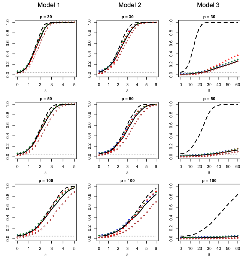
Here, we compare the performance of several two-sample tests available in the literature for high-dimensional data with the ZGZC2020 test and the SS test via several simulation models. The sample sizes for the two samples are taken as and , while the values of the dimension considered are 30, 50 and 100. When is 30 or 50, the sample sizes and are similar to the dimension ; larger than the dimension for and smaller or equal to the dimension when . However, for , and are substantially smaller than the dimension. The lowest value of considered here is not too small compared to the sample sizes, the sample covariance matrix would be invertible, but high-dimensional methods can be applied as well. For the two larger values of , the sample covariance matrix cannot be inverted but high-dimensional methods can be applied justifiably. For the underlying distributions of the samples, we consider three simulation models as described below. One of them is Gaussian, one is non-Gaussian but with finite variance and the third one is the multivariate Cauchy distribution, a heavy tailed non-Gaussian distribution with non-existent expectation.
Let with . Recall the descriptions of the probability measures and from section 3. We consider three choices of :
-
•
Model 1: is , the -dimensional zero-mean Gaussian distribution with covariance ,
-
•
Model 2: is , the -dimensional distribution with degree of freedom 4, location vector and scale matrix ,
-
•
Model 3: is , the -dimensional Cauchy distribution with location vector and scale matrix .
Let and . For each of the three models, we choose the shifts and , where is a real number.
Both Model 2 and Model 3 are comprised of non-Gaussian distributions with heavy tails. Model 2 has up to third order moments while no moment exists for the distribution in Model 3.
When , the null hypothesis (2) is satisfied, whereas the disparity between the two populations increases as is increased. So, we vary on a grid of values from 0 to some positive numbers and estimate the powers of the tests for each value of , and thus generate estimated power curves of the tests over the corresponding ranges of . We consider different values of and fix the sizes of the two groups to focus on how the powers of the tests change with .
The distributions in Models 1 and 2 are either identical or very similar to the distributions considered in Models 1 and 2 in subsection 3.1 in [27]. The expression of the shifts are also the same, however, the values of considered and the values of the dimension and the sample sizes and are different. We choose these models because of their simplicity and convenience of comparison of the performances of the ZGZC2020 test by [27] and our proposed SS test, along with several other tests from the literature. We consider Model 3 in addition to investigate the performances of the ZGZC2020 test and the other tests from the literature under significant departure from Gaussianity, so much so that the moments required for the theoretical validity of those tests are non-existent, while the proposed SS test does not require the existence of population moments.
From the literature of two-sample tests for high-dimensional data, we consider the tests by [2], [7], [12], [10] and [23], and denote them as BS1996 ([2]), CLX2014 ([7]), CQ2010 ([12]), CLZ2014 ([10, 11]) and SD2008 ([23]) tests. All these tests are implemented from the ‘highmean’ package in R ([21]).
For the combinations of the three models and the three values of , we first estimate the sizes of all the tests based on 1000 independent replications at the nominal level of 5%. The estimated sizes are reported in Table 1.
| Model | ZGZC2020 | SS | BS1996 | CLX2014 | CQ2010 | CLZ2014 | SD2008 | |
|---|---|---|---|---|---|---|---|---|
| 1 | 30 | 0.049 | 0.045 | 0.069 | 0.041 | 0.070 | 0.128 | 0.031 |
| 1 | 50 | 0.046 | 0.044 | 0.063 | 0.029 | 0.065 | 0.155 | 0.026 |
| 1 | 100 | 0.054 | 0.050 | 0.072 | 0.040 | 0.070 | 0.195 | 0.019 |
| 2 | 30 | 0.056 | 0.049 | 0.074 | 0.032 | 0.073 | 0.160 | 0.026 |
| 2 | 50 | 0.063 | 0.059 | 0.074 | 0.034 | 0.073 | 0.156 | 0.032 |
| 2 | 100 | 0.051 | 0.051 | 0.061 | 0.023 | 0.062 | 0.185 | 0.020 |
| 3 | 30 | 0.010 | 0.047 | 0.017 | 0.001 | 0.017 | 0.116 | 0.006 |
| 3 | 50 | 0.015 | 0.057 | 0.025 | 0.000 | 0.021 | 0.154 | 0.002 |
| 3 | 100 | 0.016 | 0.050 | 0.017 | 0.000 | 0.017 | 0.214 | 0.000 |
It can be observed in Table 1 that for all the models and values of , the estimated sizes of the SS test are close to the nominal level of 5%. The estimated sizes of the ZGZC2020 test are close to the nominal level in Models 1 and 2, but significantly smaller than the nominal level for the non-Gaussian distribution in Model 3. The estimated sizes of the BS1996 test and the CQ2010 test are usually slightly larger than the nominal level of 5% in the majority of cases in Models 1 and 2, but quite small compared to the nominal level in Model 3. The estimated sizes of the CLX2014 test are usually not far from the nominal level except in Model 3, where it is almost 0. The estimated sizes of the SD2008 test are somewhat smaller than the nominal level throughout Models 1 and 2, and become close to zero in Model 3. The estimated sizes of the CLZ2014 test are always very higher than the nominal level irrespective of the models and values of , its lowest estimated size being almost 12%.
The above observations indicate that the SS test has satisfactory sizes irrespective of Gaussianity or non-Gaussianity or values of . The ZGZC2020 test has satisfactory sizes in the Gaussian distribution or the non-Gaussian distribution when the moment assumptions of its validity are satisfied, but it fails to have proper size in case the sample arises from a non-Gaussian distribution not satisfying the moment conditions of its theoretical validity. The estimated sizes of the other tests are generally not so close to the nominal level compared to those of the ZGZC2020 test and the SS test.
Next, we proceed to demonstrate the estimated powers of the tests. Since the CLZ2014 test is so improperly sized, we drop it from the power comparison. As mentioned before, by varying the value of within a range from 0 to a positive number, we generate estimated power curves of the tests. For the nine total combinations of the three models and three values of , we get in total nine plots, which we present together in Figure 1. Each column in Figure 1 corresponds to one of the models, which is mentioned at the top of the figure, and the values of for each of the plot are mentioned in the headings of the individual plots. Within each plot, the estimated power curves of the tests are plotted against the values of .
From the plots in Figure 1, it can be observed that the estimated power curve of the SS test is almost uniformly higher than all the other tests except the BS1996 test and the CQ2010 test for small to moderate values of , irrespective of Gaussian or non-Gaussian distributions, although for the Gaussian distribution, the difference between the estimated powers of the SS test and the best performing tests among the rest is quite narrow. For small to moderate values of too, the estimated powers of the SS test is very close to those of the BS1996 test and the CQ2010 test. Also, similar to what was observed in Table 1, for , which corresponds to the null hypothesis being true, the estimated powers of the BS1996 test and the CQ2010 test are slightly but noticeably higher than the nominal level of 5%. This perhaps contributes to the head-start of their power curves against the SS test over , which vanishes gradually as becomes larger. The difference between the power curves of the SS test and the other tests increases in the non-Gaussian distribution in Model 2. However, in Model 3, the difference between the powers of the SS test and all other tests is quite stark. The ZGZC2020 test also performs well in Models 1 and 2, but not in Model 3. The powers of all the tests decrease as increases, and the difference between the power of the SS test and the other tests also increases with .
The overall finding from the plots in Figure 1 indicates the utility of the SS test irrespective of the Gaussianity or non-Gaussianity of the underlying distributions. Whether the magnitude of is similar to the sample size or considerably larger, the SS test is observed to perform well and almost uniformly beating all the other tests if one accounts for the proper size of the tests at the nominal level. Moreover, for a non-Gaussian distribution where the moment conditions for the validity of other tests do not hold, the difference between the performances of the SS tests and all the other tests is profound.
4.2 Comparison with multivariate tests
Recall that the ZGZC2020 test and the SS test do not normalize the test statistics with the respective inverses of the corresponding sample covariance matrices. Tests for multivariate data almost always involve normalizing with some sample covariance matrices, which makes the tests scale invariant, and as a further consequence the null distributions of those tests are usually free of any population parameters except the dimension, and the sample size for non-asymptotic tests. Evidently, the ZGZC2020 test and the SS test are not scale invariant. However, it is of interest to investigate whether this affects their performance compared to their normalized counterparts in multivariate data. This would be further of interest because to propose these tests to be employed irrespective of the dimension of the sample, for both small values of and large values of , it would be required of them to have satisfactory performance for small values of too. We investigated their performance for large in the previous subsection, and here we compare their performances against the Hotelling’s test and the test by [13] for small . We denote the Hotelling’s test as the HT2 test and the test by [13] as the CM1997 test.
Here again, we consider the same three cases of as in subsection 4.1 and like before, we take and . However, we now fix . So, here, in Model 1, is a bivariate Gaussian distribution with zero mean and covariance matrix given by . In Model 2 and Model 3, is the corresponding bivariate distribution and the bivariate Cauchy distribution, respectively. However, we change the value of the vector and consider two cases as given below:
-
•
Case 1: ,
-
•
Case 2: .
For each of these two cases, we choose the shifts and , where is a real number, like in subsection 4.1. The value corresponds to the null hypothesis (2) being true. Like before, we take the values of on a grid between 0 and some suitable positive numbers to generate estimated power curves of the tests.
| Model | ZGZC2020 | HT2 | SS | CM1997 |
|---|---|---|---|---|
| 1 | 0.060 | 0.049 | 0.057 | 0.049 |
| 2 | 0.054 | 0.050 | 0.060 | 0.049 |
| 3 | 0.018 | 0.012 | 0.054 | 0.048 |
In Table 2, the estimated sizes of the ZGZC2020, HT2, SS and CM1997 tests are presented for all three models. It should be noted that here the HT2 test is an exact non-asymptotic test, while the other three tests are asymptotic tests. It can be seen from this table that the estimated sizes for all the tests are close to the nominal level in Models 1 and 2. However, in Model 3, the estimated sizes of the ZGZC2020 test and the HT2 test are considerably different from the nominal level, yet the estimated sizes of the SS test and the CM1997 test are again close to the nominal level. This indicates that significant departure from Gaussianity similarly affects the ZGZC2020 test and the HT2 test, while the SS test and the CM1997 test remain comparably unaffected.
Next, we present the estimated power curves in Figure 2. Here, six plots are presented accounting for the six combinations of the two cases of the shifts and the three models. Each column of plots in Figure 2 corresponds to one of the models, mentioned at the top of the respective columns, while each row corresponds to one of the cases as depicted on the left sides of the corresponding columns.
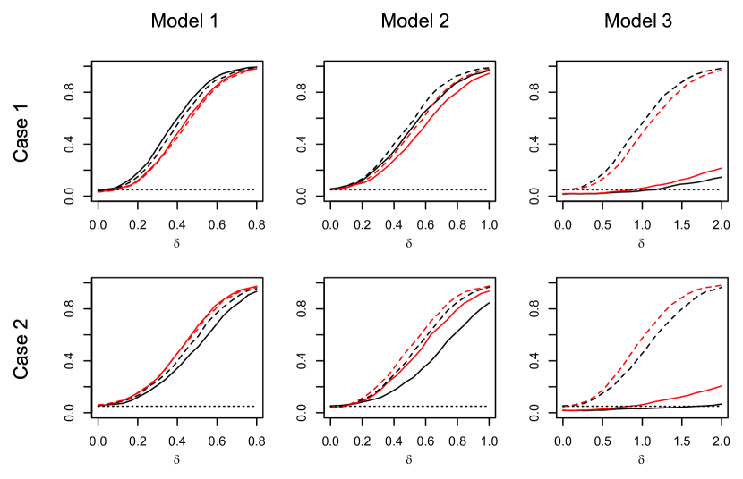
In Figure 2, it can be observed that for Case 1, the un-normalized tests ZGZC2020 and SS have higher estimated power than their normalized counterparts, namely, the HT2 test and the CM1997 test, uniformly over the range of . In Model 1 in Case 1, although the underlying distribution is Gaussian, both the ZGZC2020 test and the SS test have higher estimated power than the HT2 test. This is in spite of the fact that the HT2 test is an exact non-asymptotic test for Gaussian distributions and it is the most powerful invariant test. In Case 2, however, all the normalized tests have uniformly higher estimated power compared to the un-normalized counterparts. In both Case 1 and Case 2, the estimated power curve of the SS test is either higher or coincides with that of the ZGZC2020 test except in Model 1 in Case 1, where the ZGZC2020 test has narrowly higher power than the SS test.
4.3 Analysis of real data
We analyze the colon data available at http://genomics-pubs.princeton.edu/oncology/affydata/index.html. This dataset was first analyzed in [1] and later in many other works including [27]. It contains the expression values of 2000 genes from 62 samples of human colon tissue, 22 are from normal tissue and 40 are from tumor tissue. We are interested in testing whether the gene expression values differ between normal and tumor tissue. So, we have , and . We consider the ZGZC2020 test, the SS test, the BS1996 test, the CLX2014 test, the CQ2010 test and the SD2008 test. The p-values obtained are presented in the first row of Table 3. It can be observed that several p-values are quite small, but even among them, the p-value for the SS test is the closest to zero.
Second row: Average of p-values in the colon data with , p-values are averages over 50 blocks.
| ZGZC2020 | SS | BS1996 | CLX2014 | CQ2010 | SD2008 |
|---|---|---|---|---|---|
| 6.259680e-04 | 0.000000e+00 | 4.002116e-07 | 9.264269e-07 | 1.273052e-07 | 2.702844e-01 |
| 0.03967578 | 0.01588000 | 0.03919005 | 0.08038538 | 0.03124023 | 0.15816933 |
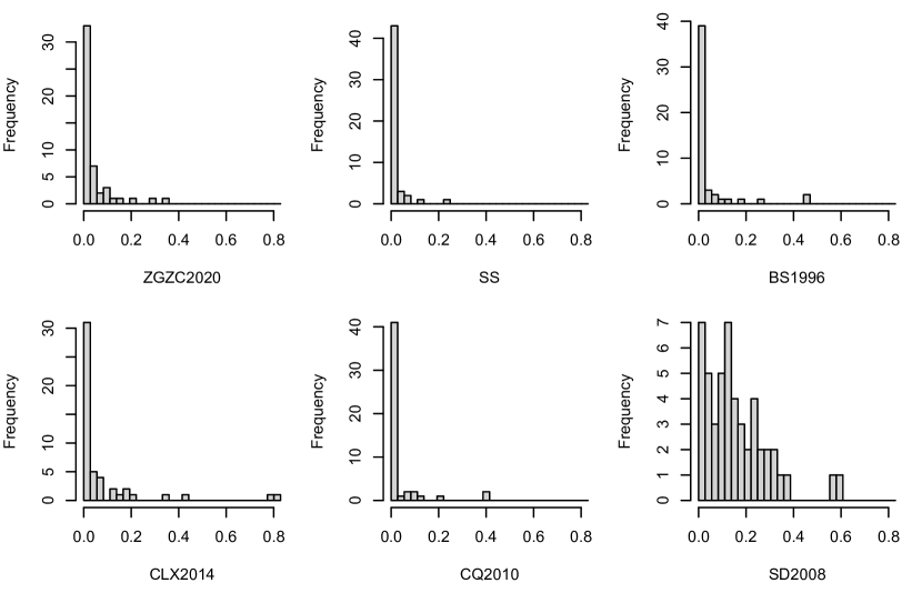
Next, we are interested in observing the p-values of the tests when the dimension is closer in magnitude to either of the sample sizes and . To implement this, we partition the data matrix by taking blocks of 40 consecutive columns. This way, we have 50 data matrices each with , and . So, here the magnitude of is comparable to the sample size. We present the histogram of the 50 p-values for each of the tests in Figure 3. The averages of the p-values are presented in the second row of Table 3. Although the p-value of the SS test was the smallest in the first row of Table 3, most of the other p-values were also nearly zero, and it was difficult to conclude that one of the tests has higher statistical power compared to the other. However, as the value of becomes lower and comparable to the magnitude of and in the study presented in the second row of Table 3, the p-values of all the tests increase. In that case, from the second row of Table 3, it can be seen that the SS test has the lowest average p-value. In Figure 3 too, it can be observed that the p-values of the SS test are concentrated closest to zero. This indicates that the SS test has indeed higher statistical power compared to the other tests carried out on this data.
5 Concluding remarks
In this work, we have proposed a new notion of convergence of fixed-dimensional functions of high-dimensional random vectors, which is uniform over the dimension of the aforementioned random vectors. This notion of convergence can be employed to derive asymptotic null distributions of tests, which are applicable for both low-dimensional and high-dimensional data. We have utilized this notion of convergence to derive the asymptotic null distribution of a general class of kernel-based multi-sample tests of equality of locations. We have then considered two specific choices of the kernel, one of which yielded an existing test in the literature (denoted as the ZGZC2020 test above, proposed by [27]) and the other one gave a spatial sign-based test (denoted as the SS test). The notion of uniform-over-dimension convergence to the asymptotic null distribution is expected to yield tests which perform as good for high-dimensional data as for low-dimensional data, and we have demonstrated this fact using simulated and real data. We have shown that the SS test in particular outperforms several popular tests in the literature for high-dimensional data in both Gaussian and non-Gaussian models. We have also provided examples of low-dimensional non-Gaussian and even Gaussian models, where the SS test outperforms even the Hotelling’s test.
The applicability of the notion of uniform-over-dimension convergence on some of the common results in the usual convergence in distribution and probability is demonstrated in this work. However, many other useful results remain to be explored, e.g., the Lindeberg central limit theorem and U-statistic asymptotic results, which we have not considered in this work and intend to study subsequently. It is of interest too to study other asymptotic tests for multivariate and high-dimensional data, whether they can be implemented uniformly-over-dimension, so that they yield good performance irrespective of the dimension of the data.
Proofs of mathematical results
Proof of subsection 2.1.
For every , define by
For every and every , we have
| and | ||||
So, and are bounded functions for every with
| (3) |
Also, and are Lipschitz continuous functions, since
which implies
| (4) |
Next, for a set and a number , define . We shall establish that
| (5) |
Note that and . For , from (3) we have , so . Similarly, for , . Now, suppose if possible, for some , . This implies from the definition of that there exists with . Since , we must have for the strict inequality to hold, which implies because , and this yields . Now and together imply that , a contradiction. So, we must have for every . Similarly, it follows that for every . Therefore, we have
| (6) | ||||
So from (6), we have for every , which establishes (5). Therefore, from (5) we have, for every and any probability measure on ,
| (7) |
Next, we proceed to show that
| (8) |
Suppose, if possible, (8) is not true, which means there exists and a subsequence such that for every ,
Then, there is a sequence corresponding to such that for every ,
| (9) |
From assumption (A1), has a subsequence such that
| (10) |
for some probability measure on , and so
| (11) |
From (9), (10) and (11), we have for all sufficiently large ,
| (12) |
Now, is a decreasing sequence of sets with as , which implies
| (13) |
From (12) and (13), we have for all sufficiently large ,
| (14) |
Now, from (10) we have
| (15) |
and (14) and (15) together imply that for all sufficiently large ,
But this is a direct contradiction to the fact that is a -continuity set for all , which means for every . This establishes the validity of (8).
Proof of Theorem 1.
(i) (ii) is obvious from subsection 2.1.
(ii) (iii): It is enough to prove that every continuous function , which is zero outside of a compact set , is bounded and uniformly continuous.
Because is continuous on and 0 outside , it is bounded on (Theorem 4.15 in [22]). Next, suppose if possible, is not uniformly continuous on . Then, there is and sequences and such that as but for every . Consider the sets and . If has infinitely many elements, then there is a subsequence of and a point with as (Theorem 2.37 in [22]), otherwise, there is such that for all , with . Similarly, if has infinitely many elements, then there is a subsequence of and a point with as , and otherwise, there is such that for all , with .
Suppose has infinitely many elements. Then, as , and as from the continuity of . However, this yields for all sufficiently large , which contradicts the continuity of at . Now suppose has infinitely many elements. Using the same arguments as above, we again get a contradiction to the continuity of at . Finally, suppose and have both finitely many elements, which means for all , with , contradicting the statement that for every . Therefore, must be uniformly continuous on .
(iii) (iv): Let be a bounded and Lipschitz continuous function, and let . Given , under assumption (A1), there is a compact set such that (1) holds: for all . Define as
Note that is the same function defined in the proof of subsection 2.1 with replaced by the compact set and . So, from (3) and (4) in the proof of subsection 2.1, it follows that and is a Lipschitz continuous function. Also, from (6), it follows that for and for , where . Note that . Summarising, we have
| (16) | ||||
So, from (16), it follows that
| (17) |
Suppose . Then, for some . For with , for any , which implies , and hence . Therefore, is an open set, which implies that is closed. Further, since is a compact set, it is bounded, and hence is bounded. So, , being a closed and bounded subset of , is a compact set (Theorem 2.41 in [22]).
Since is compact, (16) implies that and are continuous functions which are 0 outside the compact set , and so from (iii) we have for all sufficiently large ,
| (18) | ||||
Note that
| (19) | ||||
Now,
| (20) |
and similarly,
| (21) |
So, (19), (20) and (21) together yield
| (22) |
Applying (17) and (18) in (22), we get for all sufficiently large ,
| for all , which implies | ||||
Since is arbitrary, we get .
(iv) (v): Under assumption (A1) and from subsection 2.1, for a set , which is a -continuity set for all and given any , we can find bounded and Lipschitz continuous functions such that and . Since are bounded and Lipschitz functions, from (iv) we have for all sufficiently large ,
| (23) |
Now,
| which implies | ||||
Hence, from (23), we have
The proof follows since is arbitrary.
(v) (i): Let be a non-negative bounded continuous function, and let . Then, for any probability measure on ,
which, by Fubini’s theorem (Theorem 18.3 in [3]), implies that
| (24) |
Since is continuous, . There can be only countably many values of such that for at least one . So, is a -continuity set for every except for countably many , which means, from (v),
| (25) |
except for countably many . Define by
Then, clearly, for every , and from (25), except for countably many . Therefore, from the bounded convergence theorem (Theorem 16.5 in [3]), we have
| (26) |
On the other hand, for every and ,
which implies
| (27) |
Hence, (26) and (27) together imply that for every non-negative bounded continuous function ,
| (28) |
Now, let be a bounded continuous function. Then, , where and . Since is bounded and continuous, both and are bounded and continuous functions, and from (28) we have
| (29) | ||||
Now, for every and ,
which implies, for every ,
| (30) |
(29) and (30) together imply that
(v) (vi): Let be a continuity point of for all . Let . Then . Since and is a continuity point of for all , for all , and hence as .
(vi) (iii): Define for . Since for every , the sets are disjoint for distinct values of , there can be at most countably many values of such that for at least one . Hence, the set
| (31) |
is at most countable. We establish below that any such that for every is a continuity point of for all .
Suppose, is not a continuity point of . Then, there is and a sequence converging to such that for all . Define the sets for . Because is a distribution function, any sequence that converges to such that for all sufficiently large , for all , one must have as . Therefore, for all sufficiently large , , and because there are only sets , there is some such that contains infinitely many elements from , i.e., has a subsequence with . Define a sequence such that for and , and consider the sets and . Since , being a subsequence of , converges to , as as well as for all , and this implies that the sequence of sets converges to . Therefore, as . Since for all , if converges to as , we must have , which implies , because .
On the other hand, if does not converge to as , there is and a subsequence of such that for all . Clearly, converges to as and for all . Now, define the sets for . Using similar argument as before, we get a subsequence of with for some . Next, define the sequence such that for and , and consider the sets and . Again using arguments similar to those used before, we get as and for all . If converges to as , we have , and this implies , since . If does not converge to as , there is and a subsequence of such that for all , converges to as and for and for all , and we repeat the same argument.
Each iteration above fixes one additional component of the resultant sequence of -dimensional vectors to the corresponding component of , and we continue the iterations if does not converge to as . If we still do not get convergence of after iterations, using the same arguments as in previous iterations, we get some and a subsequence of such that for , for all , as but for all . Now define . We have for all . Also, the sets as because converges to , which implies . But this implies that for every since . Hence, we have established that if is not a continuity point of , then for at least one .
Therefore, any such that for every is a continuity point of for all , where is described in (31).
Next, let and be such that , and for every . Let . We proceed to show that under (vi), as . Let be such that each is either or , and let denote the number of ’s in the components of the vector . So, there are possible values of the vector depending on the values of and . Let be defined as , where and . Clearly, for any probability measure on , . Also, , where the sum is over all values of . Hence, , where . Since and , we get that and , which from (vi) yields
| (32) |
as .
Let be a continuous function which is zero outside the compact set . While proving (ii) (iii) above, it was established that such a function is bounded and uniformly continuous. So, given , there is such that implies . We now construct a finite partition of in hyper-rectangles such that for every vertex of any of the hyper-rectangles, for , and hence every such vertex is a continuity point of for all , and also, for points and lying in a hyper-rectangle, .
Since given in (31) is at most countable, is dense in . Because is compact and is dense, there is such that and is a subset of the hyper-rectangle . Take , and given with , choose such that , and . If , take . Such a sequence of ’s can be chosen because is dense. Also, by the method of construction, the sequence is finite and can have at most many elements. Let be the number of elements in . Then, the collection of intervals partitions , and for . Consider the corresponding partition of formed by hyper-rectangles with vertices such that for some and for . Clearly, this partition has at most many hyper-rectangles, which are formed by taking products of the intervals . Now, from this partition of , we remove those hyper-rectangles such that . Let hyper-rectangles remain in the collection, and we denote them as . The collection provides a partition of in hyper-rectangles such that for every vertex of any of the hyper-rectangles, for . If and lie in a hyper-rectangle, for every , and hence . Each is of the form , and define such that for , i.e., is the mid-point of the hyper-rectangle . In addition, from (32) we get that
| (33) |
Now, corresponding to , we define another function in the following way. For any , if , then define . If , then there is exactly one hyper-rectangle which contains , because ’s are disjoint, and define for such an as , where is the mid-point of . Note that for , . And for for any , , since . Therefore,
| (34) |
On the other hand, we have
which, from (33), implies that
| (35) |
as . Using (34) and (35), we get
for all sufficiently large . This establishes (vi) (iii) since is arbitrary. ∎
We need the following result (Lemma 8.7.1 in [20]) for proving the uniform-over- Lévy’s continuity theorem.
Lemma \thelemma ([20]).
For and ,
Proof of Theorem 2.
Let and be random vectors with distributions and , respectively. Suppose uniformly over . For any fixed , and are bounded continuous functions of . Hence, from subsection 2.1, we have
Therefore,
Next, assume as . We shall show that for any continuous function that is zero outside a compact set, we have as . Define and . Note that
which implies
Since and are non-negative functions of , it is enough to consider as a non-negative continuous function which is zero outside a compact set. If is identically 0, the assertion as is vacuously satisfied. So, without loss of generality, we assume that is a non-negative and non-zero continuous function which is zero outside a compact set.
Let be fixed. As is continuous on a compact set, it is uniformly continuous, so we can find such that implies .
Let be a -dimensional random vector independent of and for all and and follow the distribution, where is small such that . We have
| (36) |
Now,
| (37) |
Similarly,
| (38) |
Next, using Proofs of mathematical results and Fubini’s theorem, we have
| (39) |
where and are independent random vectors, with following the distribution and has the density .
Proof of Theorem 3.
For any bounded and continuous , the composite function defined by is bounded and continuous. Since uniformly-over-, from subsection 2.1 we have
as , which implies that uniformly-over-. ∎
Proof of subsection 2.2.
Let be a bounded and uniformly continuous function. So, given any , there is such that implies that . Therefore, implies that for any probability measure on ,
| (43) |
Since is a bounded sequence, we can construct a finite collection such that for every , for at least one . Let denote the number closest to . Therefore, using (43), we get
which implies that for every and every ,
| (44) |
Next, define by for . Then, is a bounded and uniformly continuous function for every , and from (ii) in Theorem 1 we have
as . Therefore, there is such that for all ,
| (45) |
On the other hand, we have for every ,
which, from an application of (44) and (45) together, yields
for every and every . Hence, for all ,
| (46) |
Let . Now, . So, implies , and using this fact we have
which implies
| (47) |
Since uniformly-over-, from subsection 2.2 we get that there is such that for all , . Hence, from (47) we have
| (48) |
for all . Using (46) and (48), we get that for all ,
| (49) |
Since is arbitrary, (49) along with (ii) in Theorem 1 imply that uniformly-over-. ∎
Proof of Theorem 4.
From subsection 2.2, we get that uniformly-over-. Now, to prove (a), define by . Then, from the continuity of and Theorem 3, we get uniformly-over-. To prove (b), define by , and we similarly get uniformly-over-.
Next, let and define by if and if . Clearly, is a continuous function on . Also, if and only if , and in particular for any and every , since for every . Hence, for any bounded continuous function ,
which implies
| (50) |
Now, implies that . Hence, for every and . So, from (50) we have
| (51) |
Consider any . Since from subsection 2.2 we have uniformly-over- and the composite function defined by is bounded and continuous, from subsection 2.1 we get that there is an integer such that such for all , we have . Also, from subsection 2.2 we get that there is another integer such that for all , we have . Therefore, from (51) we get that for all ,
Since is arbitrary and is any bounded continuous function, the above inequality establishes (c). ∎
Proof of section 3.
Let be the eigenvectors of corresponding to the eigenvalues . By the Karhunen-Loeve expansion, we have
for , where are random variables uncorrelated over and independent over , with and for all and . Denote . Then, , and
Define
where . Let and denote the characteristic functions of and , respectively. Then, using inequality () in [3, p. 343], we have
| (52) |
and (52) yields
| (53) |
From (A.1) in [27], we get
| (54) |
for some positive constant and for every and . Then, from (53) and (54), we get
| (55) |
Since by assumption, is bounded as , we have for and ,
| (56) |
for all . Now, for any fixed and , we get from the central limit theorem and the continuous mapping theorem that
as , where are independent chi square random variables with degree of freedom 1. Let denote the characteristic function of . Then, for all which depends on , we have
| (57) |
Next, let denote the characteristic function of . Then, using arguments similar to those used to establish (56), we get that for all ,
| (58) |
Combining (56), (57) and (58), we get
| (59) |
for all and all . Now, using the central limit theorem and the continuous mapping theorem, we get that for every fixed , there is such that
| (60) |
for every . Taking , we get that
which completes the proof. ∎
Proof of Theorem 5.
Define , where and are independent -dimensional random vectors. Define
| and | ||||
where . Then,
Next, define
We have
| (61) |
It follows from (61) that for every case other than and , we have
| (62) |
Note that . Using (62), we have
| (63) |
From (62), we get
| (64) |
uniformly-over- as . Next, it can be verified that
| (65) |
Since for all as , from (65), we have for all and ,
| (66) |
∎
Proof of Theorem 6.
Under in (2), it follows from Theorem 5 that for every , the size of the level kernel-based test converges to as uniformly-over-.
Since for all , as uniformly-over-, if there is such that for every , we have as uniformly-over- for that , and this implies as uniformly-over-. So, the power of the test converges to 1 as uniformly-over-. ∎
References
- [1] {barticle}[author] \bauthor\bsnmAlon, \bfnmUri\binitsU., \bauthor\bsnmBarkai, \bfnmNaama\binitsN., \bauthor\bsnmNotterman, \bfnmDaniel A\binitsD. A., \bauthor\bsnmGish, \bfnmKurt\binitsK., \bauthor\bsnmYbarra, \bfnmSuzanne\binitsS., \bauthor\bsnmMack, \bfnmDaniel\binitsD. and \bauthor\bsnmLevine, \bfnmArnold J\binitsA. J. (\byear1999). \btitleBroad patterns of gene expression revealed by clustering analysis of tumor and normal colon tissues probed by oligonucleotide arrays. \bjournalProceedings of the National Academy of Sciences \bvolume96 \bpages6745–6750. \endbibitem
- [2] {barticle}[author] \bauthor\bsnmBai, \bfnmZhidong\binitsZ. and \bauthor\bsnmSaranadasa, \bfnmHewa\binitsH. (\byear1996). \btitleEffect of high dimension: by an example of a two sample problem. \bjournalStatistica Sinica \bvolume6 \bpages311–329. \endbibitem
- [3] {bbook}[author] \bauthor\bsnmBillingsley, \bfnmPatrick\binitsP. (\byear2008). \btitleProbability and Measure. \bpublisherJohn Wiley & Sons. \endbibitem
- [4] {bbook}[author] \bauthor\bsnmBillingsley, \bfnmPatrick\binitsP. (\byear2013). \btitleConvergence of Probability Measures. \bpublisherJohn Wiley & Sons. \endbibitem
- [5] {barticle}[author] \bauthor\bsnmBiswas, \bfnmMunmun\binitsM. and \bauthor\bsnmGhosh, \bfnmAnil K\binitsA. K. (\byear2014). \btitleA nonparametric two-sample test applicable to high dimensional data. \bjournalJournal of Multivariate Analysis \bvolume123 \bpages160–171. \endbibitem
- [6] {barticle}[author] \bauthor\bsnmBühlmann, \bfnmPeter\binitsP., \bauthor\bsnmKalisch, \bfnmMarkus\binitsM. and \bauthor\bsnmMeier, \bfnmLukas\binitsL. (\byear2014). \btitleHigh-dimensional statistics with a view toward applications in biology. \bjournalAnnual Review of Statistics and Its Application \bvolume1 \bpages255–278. \endbibitem
- [7] {barticle}[author] \bauthor\bsnmCai, \bfnmT Tony\binitsT. T., \bauthor\bsnmLiu, \bfnmWeidong\binitsW. and \bauthor\bsnmXia, \bfnmYin\binitsY. (\byear2014). \btitleTwo-sample test of high dimensional means under dependence. \bjournalJournal of the Royal Statistical Society Series B: Statistical Methodology \bvolume76 \bpages349–372. \endbibitem
- [8] {barticle}[author] \bauthor\bsnmCarvalho, \bfnmCarlos M\binitsC. M., \bauthor\bsnmChang, \bfnmJeffrey\binitsJ., \bauthor\bsnmLucas, \bfnmJoseph E\binitsJ. E., \bauthor\bsnmNevins, \bfnmJoseph R\binitsJ. R., \bauthor\bsnmWang, \bfnmQuanli\binitsQ. and \bauthor\bsnmWest, \bfnmMike\binitsM. (\byear2008). \btitleHigh-dimensional sparse factor modeling: Applications in gene expression genomics. \bjournalJournal of the American Statistical Association \bvolume103 \bpages1438–1456. \endbibitem
- [9] {barticle}[author] \bauthor\bsnmChakraborty, \bfnmAnirvan\binitsA. and \bauthor\bsnmChaudhuri, \bfnmProbal\binitsP. (\byear2017). \btitleTests for high-dimensional data based on means, spatial signs and spatial ranks. \bjournalThe Annals of Statistics \bvolume45 \bpages771–799. \endbibitem
- [10] {barticle}[author] \bauthor\bsnmChen, \bfnmSong Xi\binitsS. X., \bauthor\bsnmLi, \bfnmJun\binitsJ. and \bauthor\bsnmZhong, \bfnmPing-Shou\binitsP.-S. (\byear2014). \btitleTwo-sample tests for high dimensional means with thresholding and data transformation. \bjournalarXiv preprint arXiv:1410.2848. \endbibitem
- [11] {barticle}[author] \bauthor\bsnmChen, \bfnmSong Xi\binitsS. X., \bauthor\bsnmLi, \bfnmJun\binitsJ. and \bauthor\bsnmZhong, \bfnmPing-Shou\binitsP.-S. (\byear2019). \btitleTwo-sample and ANOVA tests for high dimensional means. \bjournalThe Annals of Statistics \bvolume47 \bpages1443–1474. \endbibitem
- [12] {barticle}[author] \bauthor\bsnmChen, \bfnmSong Xi\binitsS. X. and \bauthor\bsnmQin, \bfnmYing-Li\binitsY.-L. (\byear2010). \btitleA two-sample test for high-dimensional data with applications to gene-set testing. \bjournalThe Annals of Statistics \bvolume38 \bpages808–835. \endbibitem
- [13] {barticle}[author] \bauthor\bsnmChoi, \bfnmKyungmee\binitsK. and \bauthor\bsnmMarden, \bfnmJohn\binitsJ. (\byear1997). \btitleAn approach to multivariate rank tests in multivariate analysis of variance. \bjournalJournal of the American Statistical Association \bvolume92 \bpages1581–1590. \endbibitem
- [14] {barticle}[author] \bauthor\bsnmChowdhury, \bfnmJoydeep\binitsJ. and \bauthor\bsnmChaudhuri, \bfnmProbal\binitsP. (\byear2022). \btitleMulti-sample comparison using spatial signs for infinite dimensional data. \bjournalElectronic Journal of Statistics \bvolume16 \bpages4636–4678. \endbibitem
- [15] {barticle}[author] \bauthor\bsnmFeng, \bfnmLong\binitsL., \bauthor\bsnmZou, \bfnmChangliang\binitsC. and \bauthor\bsnmWang, \bfnmZhaojun\binitsZ. (\byear2016). \btitleMultivariate-sign-based high-dimensional tests for the two-sample location problem. \bjournalJournal of the American Statistical Association \bvolume111 \bpages721–735. \endbibitem
- [16] {barticle}[author] \bauthor\bsnmGoeman, \bfnmJelle J\binitsJ. J., \bauthor\bsnmVan De Geer, \bfnmSara A\binitsS. A. and \bauthor\bsnmVan Houwelingen, \bfnmHans C\binitsH. C. (\byear2006). \btitleTesting against a high dimensional alternative. \bjournalJournal of the Royal Statistical Society Series B: Statistical Methodology \bvolume68 \bpages477–493. \endbibitem
- [17] {barticle}[author] \bauthor\bsnmHu, \bfnmZongliang\binitsZ., \bauthor\bsnmTong, \bfnmTiejun\binitsT. and \bauthor\bsnmGenton, \bfnmMarc G\binitsM. G. (\byear2022). \btitleA pairwise Hotelling method for testing high-dimensional mean vectors. \bjournalStatistica Sinica. \endbibitem
- [18] {barticle}[author] \bauthor\bsnmJavanmard, \bfnmAdel\binitsA. and \bauthor\bsnmMontanari, \bfnmAndrea\binitsA. (\byear2014). \btitleConfidence intervals and hypothesis testing for high-dimensional regression. \bjournalThe Journal of Machine Learning Research \bvolume15 \bpages2869–2909. \endbibitem
- [19] {barticle}[author] \bauthor\bsnmLange, \bfnmKenneth\binitsK., \bauthor\bsnmPapp, \bfnmJeanette C\binitsJ. C., \bauthor\bsnmSinsheimer, \bfnmJanet S\binitsJ. S. and \bauthor\bsnmSobel, \bfnmEric M\binitsE. M. (\byear2014). \btitleNext-generation statistical genetics: modeling, penalization, and optimization in high-dimensional data. \bjournalAnnual Review of Statistics and its Application \bvolume1 \bpages279–300. \endbibitem
- [20] {bbook}[author] \bauthor\bsnmLebanon, \bfnmGuy\binitsG. (\byear2012). \btitleProbability: The Analysis of Data. \bpublisherCreateSpace Independent Publishing Platform \bnotehttp://theanalysisofdata.com/probability/0_2.html. \endbibitem
- [21] {bmanual}[author] \bauthor\bsnmLin, \bfnmLifeng\binitsL. and \bauthor\bsnmPan, \bfnmWei\binitsW. (\byear2016). \btitlehighmean: Two-Sample Tests for High-Dimensional Mean Vectors. \bnoteR package version 3.0. \endbibitem
- [22] {bbook}[author] \bauthor\bsnmRudin, \bfnmWalter\binitsW. (\byear1976). \btitlePrinciples of mathematical analysis, \bedition3 ed. \bpublisherMcGraw-Hill Publishing Company. \endbibitem
- [23] {barticle}[author] \bauthor\bsnmSrivastava, \bfnmMuni S\binitsM. S. and \bauthor\bsnmDu, \bfnmMeng\binitsM. (\byear2008). \btitleA test for the mean vector with fewer observations than the dimension. \bjournalJournal of Multivariate Analysis \bvolume99 \bpages386–402. \endbibitem
- [24] {barticle}[author] \bauthor\bsnmSrivastava, \bfnmMuni S\binitsM. S., \bauthor\bsnmKatayama, \bfnmShota\binitsS. and \bauthor\bsnmKano, \bfnmYutaka\binitsY. (\byear2013). \btitleA two sample test in high dimensional data. \bjournalJournal of Multivariate Analysis \bvolume114 \bpages349–358. \endbibitem
- [25] {barticle}[author] \bauthor\bsnmWang, \bfnmLan\binitsL., \bauthor\bsnmPeng, \bfnmBo\binitsB. and \bauthor\bsnmLi, \bfnmRunze\binitsR. (\byear2015). \btitleA high-dimensional nonparametric multivariate test for mean vector. \bjournalJournal of the American Statistical Association \bvolume110 \bpages1658–1669. \endbibitem
- [26] {barticle}[author] \bauthor\bsnmWang, \bfnmY\binitsY., \bauthor\bsnmMiller, \bfnmDJ\binitsD. and \bauthor\bsnmClarke, \bfnmR\binitsR. (\byear2008). \btitleApproaches to working in high-dimensional data spaces: gene expression microarrays. \bjournalBritish Journal of Cancer \bvolume98 \bpages1023–1028. \endbibitem
- [27] {barticle}[author] \bauthor\bsnmZhang, \bfnmJin-Ting\binitsJ.-T., \bauthor\bsnmGuo, \bfnmJia\binitsJ., \bauthor\bsnmZhou, \bfnmBu\binitsB. and \bauthor\bsnmCheng, \bfnmMing-Yen\binitsM.-Y. (\byear2020). \btitleA simple two-sample test in high dimensions based on -norm. \bjournalJournal of the American Statistical Association \bvolume115 \bpages1011–1027. \endbibitem