Enhancing Quantum Entanglement in Bipartite Systems: Leveraging Optimal Control and Physics-Informed Neural Networks

Abstract

Quantum entanglement stands at the forefront of quantum information science, heralding new paradigms in quantum communication, computation, and cryptography. This paper introduces a quantum optimal control approach by focusing on entanglement measures rather than targeting predefined maximally entangled states. Leveraging the indirect Pontryagin Minimum Principle, we formulate an optimal control problem centered on maximizing an enhanced lower bound of the entanglement measure within a shortest timeframe in the presence of input constraints. We derive optimality conditions based on Pontryagin’s Minimum Principle tailored for a matrix-valued dynamic control system and tackle the resulting boundary value problem through a Physics-Informed Neural Network, which is adept at handling differential matrix equations. The proposed strategy not only refines the process of generating entangled states but also introduces a method with increased sensitivity in detecting entangled states, thereby overcoming the limitations of conventional concurrence estimation.

I Introduction

Quantum entanglement, a central tenet of quantum mechanics, manifests itself as a unique phenomenon in which two or more particles become intricately correlated. Remarkably, this includes the properties of one particle instantaneously influences those of another, transcending spatial distances. In the realm of quantum information, entanglement is not merely a fascinating aspect of quantum systems but is hailed as a valuable resource. This perspective has fueled a keen interest in the pursuit of maximally entangled quantum states (see an illustration in Fig. 1).

As researchers delve deeper into the manipulation of quantum states, the control of entanglement dynamics has emerged as a pivotal objective, promising unparalleled opportunities for the effective utilization and optimization of quantum resources. The field has witnessed significant developments, unveiling the fundamental principles governing entanglement and providing a roadmap for steering its evolution with precision. The quest to control entanglement dynamics is driven by the potential to unlock new horizons in quantum information processing. In this context, the entangled states form the basis for transformative applications in quantum communication [1], computation [2], and cryptographic protocols [3].

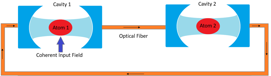
Figure 1: The model depicts a bipartite system consisting of two atoms positioned within separate cavities, and interconnected by a closed-loop optical fiber. A coherent input field is applied into Cavity 1, influencing Atom 1, and the resulting light paths are routed through the optical fibers to Cavity 2 and back. The closed-loop setup introduces additional pathway for quantum entanglement to circulate among the two atoms.

From the standpoint of control theory, the generation of Maximally Entangled States (MES) encompasses both open-loop and feedback methods. In both approaches, a specified MES, such as a Bell state $\left|GHZ\right\rangle$, or $\left|W\right\rangle$ state, serves as the target state $\rho_{d}$. Subsequently, a control law is devised to drive the system state $\rho(t)$ to $\rho_{d}$. However, for more complex systems, possessing many MES with unknown structures, the design of quantum control for MES generation should be rooted in the desired entanglement measure rather than a predetermined MES. In this regard, quantum Lyapunov control [4, 5], as a feedback approach and optimal control theory [6, 7, 8, 9, 10, 11], amongst open loop control methods have been indicated as proper candidates for the creation of entangled states. To the best of the author’s understanding, while optimal control has been demonstrated to be effective in maximizing entanglement, its indirect utilization remains largely untapped in this domain. Indirect optimal control, based on the calculus of variations and Pontryagin’s Minimum Principle (PMP), shows promise for addressing quantum state transfer challenges, and it may have applications in targeting MESs. Through this method, our emphasis shifts towards focusing on maximizing an entanglement measure rather than adhering to the conventional strategy of considering a predetermined target state. Furthermore, the quantitative evaluation of the entanglement employed in this study showcases a distinctive capability: it can discern entangled states that often escape detection through traditional entanglement measure estimation methods. This underscores the increased sensitivity and discriminatory power inherent in the chosen entanglement evaluation approach. In comparison to the state of the art, we have the following two main contributions:

• We delve into an entanglement measure-centric quantum optimal control approach. In the domain of quantum entanglement, our approach diverges from conventional methods by leveraging entanglement measures to inform the design of quantum control. Rather than tailoring a controller for a predetermined maximally entangled state, we employ entanglement measures, particularly an enhanced lower bound, which excels at identifying entanglement beyond the scope of conventional concurrence estimation methods.

• In addition, we pioneer the application of the indirect Pontryagin maximum principle to optimize entanglement, ushering in a new perspective for the optimal control of entanglement dynamics. In essence, this work formulates an optimal control problem that prioritizes the maximization of a robust lower bound of the entanglement measure within an optimal time frame. This problem formulation yields results that surpass existing state-of-the-art approaches.

• Lastly, we illustrate the obtained results for a closed quantum system, adhering to the Liouville-von Neumann equation, and examine the time evolution of the density operator $\rho(t)$. To this end, we extend the Physics-Informed Neural Network (PINN) method for generic differential matrix equations.

The remainder of the work is organized as follows: In Section II, we briefly recap the most highlighted entanglement monotones and measures in the literature for bipartite pure and mixed states. We then continue with the derivation of the lower bound of concurrence for an arbitrary-dimensional bipartite state in terms of lower-dimensional systems and how this lower bound is exploited as a sufficient condition for distillability of quantum entanglement. We then formulate an optimal control problem such that we maximize the lower bound of concurrence in minimum time in the presence of input constraints. We validate our results through numerical simulations in section IV. The paper ends with a conclusion and an outlook to future work.

Notation

For a general continuous-time trajectory $x$, the term $x(t)$ indicates the trajectory evaluated at a specific time $t$. For writing the conjugate transpose of a matrix (or vector), we use the superscript $\dagger$. To denote wave functions as vectors, we use the Dirac notation such that $\left|\psi\right\rangle=\sum\limits_{k=1}^{n}{{{\alpha}_{k}}\left|{{{\hat{\psi}}}_{k}}\right\rangle}$, where $|\psi\rangle$ indicates a state vector, ${\alpha}_{k}$ are the complex-valued expansion coefficients, and $|{\hat{\psi}}_{k}\rangle$ are fixed basis vectors. The notation bra is defined such that $\left\langle\psi\right|=\left|\psi\right\rangle^{\dagger}$. The quantum density operator is denoted by $\rho=\sum\limits_{j}{{{p}_{j}}\left|{{\psi}_{j}}\right\rangle\left\langle{{\psi}_{j}}\right|}$ where coefficients ${p_{j}}$ are non-negative and add up to one. For writing partial differential equations, we denote partial derivatives using $\partial$. The sign $\otimes$ indicates the tensor product. The notation $[\cdot,\cdot]$ represents a commutator. We denote the trace of a square matrix $A$ by $\Tr(A)$, and the partial trace over subsystem $B$ by $\Tr_{B}$. Throughout the paper, the imaginary unit is $i=\sqrt{-1}$. A d-dimensional Hilbert space is represented by $\mathbb{H}_{d}$, and $\mathcal{H}_{\rho}$ is the set of linear bounded operators on $\mathbb{H}_{d}$ characterized by $d\times d$ complex matrices that are positive semi-definite, Hermitian, and has trace one.

II Optimal Control based on Quantum Entanglement Measure

We consider the quantum control design for generation of maximally entangled states based on the entanglement measure rather than for a specified maximally entangled state. Specifically, the entanglement measure that we aim to maximize is the lower bound of concurrence from all known lower bounds. The control signal is designed such that the entanglement measure lower bound reaches its maximum in a minimum time.

II-A Entanglement Monotones and Measures

We delve into the fundamental concepts of entanglement theory, focusing on entanglement monotones and measures - a crucial aspect in the study of quantum entanglement. Entanglement measures are mathematical constructs that quantify the degree of entanglement within quantum states, offering valuable insights into the intricacies of quantum systems. We indicate the establishment of key criteria that entanglement measures must satisfy and explore the significance of entanglement monotones, which encapsulate essential properties for characterizing entanglement. Here is a list of possible postulates for a bipartite entanglement measure $E(\rho)$ [12, 13, 14, 15].

1. A measure $E(\rho)$ quantifies the intensity of entanglement of a state $\rho$ by mapping system density matrices to positive real numbers, i.e., $\rho\mapsto E\left(\rho\right)\in{\mathbb{R}^{+}}$.

2. $E(\rho)=0$ if and only if $\rho$ is separable, indicating no quantum entanglement.

3. $E(\rho)$ does not increase on average under Local Operations and Classical Communication (LOCC) operations. For a LOCC operation $\Lambda$, it holds that $E(\Lambda\rho)\leq E(\rho)$, ensuring the non-increase of entanglement under such operations.

4. For pure states $\rho=\left|\psi\right\rangle\left\langle\psi\right|$, the measure converges to the entropy of entanglement, aligning the entanglement measure with the von Neumann entropy for pure bipartite systems.

Any function $E(\rho)$ satisfying the first three conditions is considered monotone in relation, while functions that meet conditions 1, 2, and 4 are recognized as entanglement measures. In addition, the entanglement measure does not increase under deterministic LOCC transformations. Frequently, some authors also define entanglement measures by imposing additional criteria, including convexity, additivity, and continuity, as further detailed in [12, 13]. In [14], an entanglement measure $E(\rho)$ is characterized by an entanglement monotone function $g$ possessing the following main properties:

• Concavity: Specifically, $g(\rho)\geq\lambda g(\rho_{1})+(1-\lambda)g(\rho_{2})$ for any convex combination of states $\rho=\lambda\rho_{1}+(1-\lambda)\rho_{2}$, where $0\leq\lambda\leq 1$.

• Invariance under local unitary transformations: Meaning $g(U_{L}\rho U_{L}^{\dagger})=g(\rho)$, where $U_{L}$ is any local unitary operation.

Some key measures of entanglement include the entropy of entanglement, Renyi entropy, entanglement of formation, Negativity, and Concurrence (see Section III for the exact definition). Given the significance and widespread application of concurrence as an entanglement monotone, our paper will primarily focus on quantum entanglement through the lens of concurrence.

II-B Optimal Control Problem Statement

The role of Optimal Control

Consider a bipartite system composed of two interacting particles, each with $d$-levels (or $\mathbb{H}_{d}$). Our objective is to manipulate the state of this system to achieve a high degree of entanglement. The challenge we address is to devise optimal control strategies that can navigate the constraints imposed by the intrinsic and dissipative interactions and the initial conditions to maximize the entanglement between the two particles. Our goal is to apply Pontryagin’s Minimum principle (PMP) of optimal quantum control theory to effectively employ time-dependent external control fields to steer the system’s time evolution towards desired states that exhibit high degrees of entanglement. It means that starting from an initial state ${{\rho}_{i}}$, the target is a maximally entangled set rather than a single state, i.e., $S_{{MES}}$.

For a $d$-dimensional bipartite system, composed of two subsystems $A$ and $B$, a maximally entangled basis can be constructed using the generalized Bell states or the so-called maximally entangled states. These states can be defined as

$$|\Psi_{mn}\rangle=\frac{1}{\sqrt{d}}\sum_{j=0}^{d-1}e^{\frac{2\pi i}{d}jn}|j\rangle_{A}\otimes|(j+m)\mod d\rangle_{B}$$

Here, $|j\rangle_{A}$ and $|(j+m)\mod d\rangle_{B}$ are the computational basis states of subsystems $A$ and $B$, respectively. The term $e^{\frac{2\pi i}{d}jn}$ introduces a phase that depends on $n$, and the summation runs over all basis states from $0$ to $d-1$, creating a superposition of these states. The set of these maximally entangled states, $\{|\Psi_{mn}\rangle\}$, for $m,n\in\{0,\ldots,d-1\}$, forms a complete orthonormal basis for the $d^{2}$-dimensional Hilbert space of the bipartite system. This set can be compactly denoted as

$$S_{MES}=\{|\Psi_{mn}\rangle:m,n\in\{0,\ldots,d-1\}\}$$ (1)

Each $|\Psi_{mn}\rangle$ in $S_{MES}$ is a maximally entangled state, and for $d=2$, this set reduces to the familiar set of four Bell states in $\mathbb{H}_{4}$ [16].

Problem formulation

The design of optimal quantum controllers varies significantly based on the chosen cost functional, the formulation of the Pontryagin-Hamiltonian function, and the numerical methods employed to satisfy the PMP optimality conditions. In this context, for a general d-level quantum system described by

$$\dot{\rho}(t)=F(\rho(t),u(t)),\quad\rho(t_{0})=\rho_{0}\in\mathcal{H}_{\rho}\subset{{\mathbb{C}}^{d\times d}}$$ (2)

we specifically address a time-minimization problem, denoted as ($P$), which focuses on optimizing the duration of quantum operations within the constraints of bounded control input $u(t)$. In Section III, we particularize (2) for Liouville–von Neumann dynamics. The objective is to maximize the lower bound of the concurrence measure for entanglement, denoted as $\tau(\rho)$, in the shortest possible timeframe. The decision to maximize the tight lower bound $\tau(\rho)$ rather than direct concurrence in our optimal control framework is supported by both practical and theoretical considerations. The tight lower bound provides a more computationally tractable objective for optimization due to its formulation involving lower-dimensional projections of $\rho$. This approach simplifies the complexity inherent in high-dimensional optimization problems. The problem casts as the following:

$$(P)\left\{\begin{aligned} &\min_{t_{f}}\left\{J(t_{f})=\Gamma\,{{t}_{f}}-\tau(\rho)\right\}\\ &\text{subject to }\\ &\dot{\rho}(t)=F(\rho(t),u(t))\text{ a.e. }t\in[t_{0},t_{f}]\\ &\rho(t_{0})=\rho_{0}\in\mathcal{H}_{\rho}\\ &u\left(t\right)\in\mathcal{U}:=\left\{u\in{{L}_{\infty}^{m}}:{{\left\|u\right\|}_{\infty}}\leq{u}_{\max}\right\}\text{ a.e. }t\in[t_{0},t_{f}]\\ \end{aligned}\right.$$

where $J$ is the performance index, $\Gamma$ is a positive coefficient, and ${{t}_{f}}$ shows the free final time to be optimized. The control is represented as a measurable bounded function. In this setup, we assume that all the sets are Lebesque measurable and the functions are Lebesgue measurable and Lebesgue integrable. The goal is to obtain a pair of trajectories $\left({{\rho}^{*}},{{u}^{*}}\right)$ that is optimal in the sense that the value of the cost functional is the minimum over the set of all feasible solutions. We will explore the measurement of entanglement using concurrence, examine the concurrence’s lower bound, and discuss the distillation process for bipartite quantum states of arbitrary dimensions.

III Principal Findings and Core Insights

III-A Analysis of Quantum Entanglement by Concurrence

We present the investigation of the concept of concurrence undertaken to delineate the dynamic characteristics exhibited by bipartite systems. Consider $\mathbb{H}_{d_{1}}$ and $\mathbb{H}_{d_{2}}$ as the corresponding Hilbert spaces of systems $A$ and $B$, respectively. A bipartite pure state is given by

$$\left|\psi\right\rangle=\sum\limits_{i=1}^{d_{1}}{\sum\limits_{j=1}^{d_{2}}{{{\phi}_{ij}}}}\left|ij\right\rangle\text{ with }{\phi}_{ij}\in\mathbb{C},\quad\sum\limits_{ij}{{{\left|{{\phi}_{ij}}\right|}^{2}}=1}$$ (3)

in computational basis $\left\{\left|ij\right\rangle\right\}$ of $\mathbb{H}_{d_{1}}\otimes\mathbb{H}_{d_{2}}$. Then, the concurrence of $\left|\psi\right\rangle$ is expressed as [17]

$$C\left(\left|\psi\right\rangle\right)=\sqrt{2\left(1-\Tr\left({{\rho}_{A}}\right)^{2}\right)}$$ (4)

where $\rho_{A}=\Tr_{B}(\left|\psi\right\rangle\left\langle\psi\right|)$. Following a series of algebraic computations done in [18], $C\left(\left|\psi\right\rangle\right)$ can be further expressed as

$$C\left(\left|\psi\right\rangle\right)=2\sqrt{\sum\limits_{i<k}^{d_{1}}{\sum\limits_{j<l}^{d_{2}}{{{\left|{{\phi}_{ij}}{{\phi}_{kl}}-{{\phi}_{il}}{{\phi}_{kj}}\right|}^{2}}}}}\cdot$$ (5)

Proposition 1

Given a pure bipartite quantum state $|\psi\rangle\in\mathbb{H}_{d_{1}}\otimes\mathbb{H}_{d_{2}}$, and its unnormalized projection $|\psi_{s\otimes w}\rangle$ onto a lower-dimensional subspace $s\otimes w$, expressed as

$${{\left|\psi\right\rangle}_{s\otimes w}}=\sum\limits_{i={{i}_{1}}}^{{{i}_{s}}}{\sum\limits_{j={{j}_{1}}}^{{{j}_{w}}}{{{\phi}_{ij}}}}\left|ij\right\rangle,\quad s\in(1,d_{1}),\quad w\in(1,d_{2})$$

the concurrence $C(|\psi_{s\otimes w}\rangle)$ of the projected state can be expressed as a function of the elements of the original state $|\psi\rangle$

$$C\left({{\left|\psi\right\rangle}_{s\otimes w}}\right)=2\sqrt{\sum\limits_{{{i}_{P}}<{{i}_{k}}}^{s}{\sum\limits_{{{j}_{q}}<{{j}_{l}}}^{w}{{{\left|{{\phi}_{{{i}_{p}}{{j}_{q}}}}{{\phi}_{{{i}_{k}}{{j}_{l}}}}-{{\phi}_{{{i}_{p}}{{j}_{l}}}}{{\phi}_{{{i}_{k}}{{j}_{q}}}}\right|}^{2}}}}}$$ (6)

Proof:

The result can be found in [19]. For the sake of completeness and to facilitate understanding, we detail the result as follows. The projection $|\psi_{s\otimes w}\rangle$ onto a lower-dimensional $s\otimes w$ space is defined by selectively summing over the coefficients $\phi_{ij}$ of the original state $|\psi\rangle$. Given the definition of $|\psi_{s\otimes w}\rangle$, the concurrence $C(|\psi_{s\otimes w}\rangle)$ can be derived from the general formula for the concurrence of a bipartite pure state given in (4). For the projected state $|\psi_{s\otimes w}\rangle$, the reduced density matrix $\rho_{A_{s\otimes w}}$ can similarly be obtained by tracing out the $w$-dimensional part of the system, resulting in:

$$\rho_{A_{s\otimes w}}=\Tr_{B_{s\otimes w}}\left(|\psi_{s\otimes w}\rangle\langle\psi_{s\otimes w}|\right)$$

Substituting this into the formula for concurrence, we find:

$$C(|\psi_{s\otimes w}\rangle)=\sqrt{2\left(1-\Tr(\rho_{A_{s\otimes w}})^{2}\right)}$$

from which one obtains (6). ∎

Remark 1

The determination of the number of distinct $s\otimes w$ projected states from a given bipartite state $|\psi\rangle$ within Hilbert spaces $\mathbb{H}_{d_{1}}\otimes\mathbb{H}_{d_{2}}$, leverages fundamental combinatorial principles, i.e., combinatorial concept of selecting subsets without regard to the order. Specifically, the binomial coefficient $\binom{d_{1}}{s}$ calculates the ways to choose $s$ dimensions from an $d_{1}$-dimensional subsystem, analogous for $\binom{d_{2}}{w}$ with $d_{2}$ and $w$. The product $\binom{d_{1}}{s}\times\binom{d_{2}}{w}$ of these coefficients, yields the total distinct projections, and forms a comprehensive set of lower-dimensional representations of the original bipartite state.

Proposition 2

The concurrence squared of a pure state $|\psi_{k}\rangle$, and the concurrence squared of its projections $|\psi_{k}\rangle_{s\otimes w}$, are related by

$$C^{2}\left(|\psi_{k}\rangle\right)=\alpha_{sw}\left[\sum_{P_{sw}}C^{2}\left(|\psi_{k}\rangle_{s\otimes w}\right)\right],$$ (7)

where $\alpha_{sw}=\frac{(s-2)!(w-2)!(m-s)!(n-w)!}{(m-2)!(n-2)!}$ represents the normalization coefficient, and the summation is over all possible $s\otimes w$ projections of $|\psi_{k}\rangle$.

Proof:

A proof of (7) is obtained in [19]. For readability, we state that the concurrence squared of $|\psi_{k}\rangle$ and its $s\otimes w$ projections are related through the normalization factor $\alpha_{sw}$. This factor compensates for the combinatorial variations in selecting $s$ and $w$ dimensions from the subsystems. The summation over $\sum_{P_{sw}}C^{2}(|\psi_{k}\rangle_{s\otimes w})$ consolidates the entanglement across all projections into a unified measure, adjusted by $\alpha_{sw}$ to accurately reflect the original state’s entanglement. Thus, $\alpha_{sw}$ and the summation process ensure that $C^{2}(|\psi_{k}\rangle)$ is effectively represented through its projections’ entanglement contributions. ∎

Proposition 3

Given a mixed quantum state $\rho$, the concurrence $C(\rho)$ can be assessed through its projections onto lower-dimensional subspaces, specifically via the concurrence of unnormalized bipartite $s\otimes w$ mixed states ${{\rho}_{s\otimes w}}$. This relationship is encapsulated by

$$C(\rho_{s\otimes w})=\min\left\{\sum_{k}p_{k}C\left(|\psi_{k}\rangle_{s\otimes w}\right)\right\},$$ (8)

where the minimization is over all possible $s\otimes w$ pure-state decompositions of ${{\rho}_{s\otimes w}}=\sum\limits_{k}{{{p}_{k}}{{\left|{{\psi}_{k}}\right\rangle}_{s\otimes w}}\left\langle{{\psi}_{k}}\right|_{s\otimes w}},\quad\sum\limits_{k}{{{p}_{k}}=tr\left({{\rho}_{s\otimes w}}\right)}$.

Proof:

See [20, 19], and references therein. For readability and completeness, we include the following proof. The concurrence $C(\rho)$ for a mixed state $\rho$ is determined via the convex roof extension, which requires finding the infimum over all ensemble realizations of $\rho$, i.e.,

$$C\left(\rho\right)=\underset{\left\{{p_{k},\left|{{\psi}_{k}}\right\rangle}\right\}}{\mathop{\inf}}\,\sum\limits_{k}{p_{k}C\left(\left|{{\psi}_{k}}\right\rangle\right)}$$ (9)

This process typically involves a complex optimization problem due to the high-dimensional nature of $\rho$. To simplify this, we consider projections of $\rho$ onto lower-dimensional subspaces $s\otimes w$, resulting in the mixed state ${{\rho}_{s\otimes w}}$. Each projection reduces the complexity of the state while retaining essential information about its entanglement structure. The concurrence $C({{\rho}_{s\otimes w}})$ of these projections can be calculated more straightforwardly due to the reduced dimensionality. The critical insight is that the concurrence of $\rho$ can be approached by aggregating the concurrence measures of its lower-dimensional projections. For a mixed state $\rho$, the unnormalized bipartite $s\otimes w$ mixed states are defined as

$${{\rho}_{s\otimes w}}=A\otimes B\rho{{A}^{\dagger}}\otimes{{B}^{\dagger}},\quad A=\sum\limits_{{{i}_{p}}=1}^{s}{\left|{{i}_{p}}\right\rangle\left\langle{{i}_{p}}\right|,\quad B=\sum\limits_{{{j}_{q}}=1}^{w}{\left|{{j}_{q}}\right\rangle\left\langle{{j}_{q}}\right|}}$$

which has the matrix form of

$${{\rho}_{s\otimes w}}=\left(\begin{smallmatrix}{{\rho}_{{{i}_{p}}{{j}_{q}},{{i}_{p}}{{j}_{q}}}}&{{\rho}_{{{i}_{p}}{{j}_{q}},{{i}_{p}}{{j}_{l}}}}&{{\rho}_{{{i}_{p}}{{j}_{q}},{{i}_{k}}{{j}_{q}}}}&{{\rho}_{{{i}_{p}}{{j}_{q}},{{i}_{k}}{{j}_{l}}}}\\ {{\rho}_{{{i}_{p}}{{j}_{l}},{{i}_{p}}{{j}_{q}}}}&{{\rho}_{{{i}_{p}}{{j}_{l}},{{i}_{p}}{{j}_{l}}}}&{{\rho}_{{{i}_{p}}{{j}_{l}},{{i}_{k}}{{j}_{q}}}}&{{\rho}_{{{i}_{p}}{{j}_{l}},{{i}_{k}}{{j}_{l}}}}\\ {{\rho}_{{{i}_{k}}{{j}_{q}},{{i}_{p}}{{j}_{q}}}}&{{\rho}_{{{i}_{k}}{{j}_{q}},{{i}_{p}}{{j}_{l}}}}&{{\rho}_{{{i}_{k}}{{j}_{q}},{{i}_{k}}{{j}_{q}}}}&{{\rho}_{{{i}_{k}}{{j}_{q}},{{i}_{k}}{{j}_{l}}}}\\ {{\rho}_{{{i}_{k}}{{j}_{l}},{{i}_{p}}{{j}_{q}}}}&{{\rho}_{{{i}_{k}}{{j}_{l}},{{i}_{p}}{{j}_{l}}}}&{{\rho}_{{{i}_{k}}{{j}_{l}},{{i}_{k}}{{j}_{q}}}}&{{\rho}_{{{i}_{k}}{{j}_{l}},{{i}_{k}}{{j}_{l}}}}\\ \end{smallmatrix}\right)$$ (10)

for which the concurrence is (8). This method ensures that $C(\rho)$ is effectively quantified by considering the contributions of entanglement from all relevant lower-dimensional subspaces. ∎

Proposition 4

A tight lower bound of concurrence can be obtained by

$$\tau_{s\otimes w}(\rho)={{\alpha}_{sw}}\sum\limits_{{{P}_{sw}}}{{{C}^{2}}}\left({{\rho}_{s\otimes w}}\right)$$ (11)

Proof:

From [19], combining (7) and (8), and (9), results in

$$C^{2}\left(\rho\right)\geq{{{\alpha}_{sw}}}{{\left[\sum\limits_{{{P}_{sw}}}{{{C}^{2}}\left({{\rho}_{s\otimes w}}\right)}\right]}}$$ (12)

Inequality (12) represents an analytical lower bound of squared concurrence for bipartite mixed states. Therefore, we can deduce that

$$C^{2}\left(\rho\right)\geq\tau_{s\otimes w}(\rho)$$ (13)

∎

The lower bound indicated in (11) is a tight lower bound, and is strictly stronger in comparison with its counterparts, [20, 21]. For instance, in [20], an analytical lower bound is obtained as $\tau_{2\otimes 2}(\rho)$, which is only a special case of (13). In addition, the lower bound in (13) is an stronger criterion to detect positive partial transposition (PPT) entangled states.

III-B Entanglement Distillation

Quantum entanglement distillation is a pivotal protocol designed to counteract the adverse effects of noisy channels in quantum information processing. Its primary objective is to enhance and improve quantum entanglement, crucial for the reliable quantum information transmission. In this subsection, we present some results regarding the distillability of entangled states.

Distillability of an Entangled Mixed State

In practical terms, determining the distillability of an entangled mixed state presents a significant challenge. However, a fundamental connection between the distillability of a mixed state and its ability to be transformed into the singlet form has been revealed in [22]. Specifically, a mixed state is said to be distillable if it can be successfully distilled into the singlet form, a condition that necessarily violates the Positive Partial Transpose (PPT) criterion. This context gives rise to two distinct categories of entanglement:

• “Free” entanglement: States that can be distilled into the singlet form, making them suitable for utilization in quantum communication.

• “Bound” entanglement: States that resist conversion into the beneficial singlet form, rendering them unsuitable for quantum communication purposes.

In this regard, the lower bound of concurrence provides a concise representation of the structure of entanglement. It serves two purposes: facilitating the assessment of free entanglement, and aiding in the classification of mixed-state entanglement. Motivated by the above, we can now state the following results regarding the distillability of quantum states.

Proposition 5

Let ${{\rho}^{\otimes N}}=\underbrace{\rho\otimes\cdots\otimes\rho}_{N}$ represent the quantum state of a composite system consisting of $N$ identical subsystems, each initially described by the density matrix $\rho\in\mathbb{H}_{d_{1}}\otimes\mathbb{H}_{d_{2}}$. From the lower bound of concurrence (13), it can be deduced that $\rho$ is distillable if the following condition holds

$$\tau_{2\otimes 2}\left({{\rho}^{\otimes N}}\right)>0,\qquad N\in\mathbb{Z}^{+}$$ (14)

Proof:

See [22]. ∎

Proposition 6

The results for Proposition 5 holds also if the projectors $A$ and $B$ map ${{\rho}^{\otimes N}}$ to one 2-dimensional and one 3-dimensional space, respectively, i.e.,

$$\tau_{2\otimes 3}>0,\qquad N\in\mathbb{Z}^{+}$$ (15)

Proof:

See [22]. ∎

Proposition 7

If (14) holds, then (15) also holds, however, the inverse is not true.

Proof:

See [19]. ∎

Remark 2

One must note that not all entangled states are detected by the distillability criterion since the condition given in Proposition 5 does not detect bound entanglement, and can detect most of the free entanglement. Bound entangled states, although entangled, cannot be utilized as a resource for quantum communication tasks unlike their free entangled counterparts. Therefore, the states that satisfy the distillability condition are highly valuable in the realm of quantum information. With a sufficient quantity of such states, it becomes possible to transform them, through local operations, into any desired entangled state, thereby enabling a diversity of potential applications.

Remark 3

Note that the primary goal of mapping bipartite system to two qubits is to make the examination of entanglement easier since it is a challenging task to detect entanglement in systems with dimensions greater than $2\otimes 3$ due to lack of necessary and sufficient conditions of entanglement in these systems. However, as mentioned earlier, there exist necessary and sufficient conditions for systems of dimensions $2\otimes 2$ and $2\otimes 3$.

III-C Necessary Optimality Conditions in the form of Pontryagin Minimum Principle

In this subsection, we delve into the solution of optimal control problem expressed in II-B. We tackle the optimal control problem (P) that prioritizes minimizing time. This problem involves bounded control and aims to maximize the lower bound of concurrence. The assessment of concurrence involves mapping the bipartite system to a two-qubit system.

System dynamics

We examine the time evolution of the density operator within a closed quantum system, adhering to the Liouville-von Neumann equation:

$$\dot{\rho}(t)=-\frac{i}{\hbar}[H(u(t)),\rho(t)]$$

where the quantum mechanical Hamiltonian $H(u(t))=H_{0}+H_{C}(u(t))$ comprises of the drift $H_{0}$ and time dependent control Hamiltonian ${{H}_{C}}\left(u\left(t\right)\right)=\sum\limits_{l=1}^{m}{{{H}_{l}}{{u}_{l}}\left(t\right)}$ which indicates the interaction of the system with the control fields $u(t)$ through the interaction Hamiltonians $H_{l}$. This evolution transpires through a unitary process, denoted as $\rho(t)=U(t)\rho_{0}U^{\dagger}(t)$. The primary objective in this controlled evolution is to transfer an initial state $\rho_{0}$ utilizing the unitary operators $U(t)$ in a manner that attains a maximally entangled state. Concurrently, the entanglement measure is optimized within an optimal time frame.

Remark 4

It is crucial to note that the unitary transformation involved in $\rho_{MES}=U(t)\rho(0)U^{\dagger}(t)$ is a global operation, acting uniformly on all particles within the system. This global transformation stands distinct from a unitary local transformation, which only influences specific particles and cannot increase the overall entanglement of $\rho(0)$.

Saturation function for handling input constraints

In order to account for control constraints, certain adjustments must be incorporated into the existing formulation (see details in [23]). Initially, it is necessary to establish a new unconstrained control variable $\bar{u}(t)$ for the control constraint existing in the problem, with each input $u_{l}(t)$ falling within the interval $[u_{min},u_{max}]$. The concept involves substituting the control constraint with a smooth and monotonically increasing saturation function, such that $u=\Phi(\bar{u})$, where each entry of entry satisfies

$$\Phi_{l}(\bar{u}_{l})=u_{max}-\frac{u_{max}-u_{min}}{1+\exp(s\bar{u}_{l})},\qquad s=\frac{c}{u_{max}-u_{min}}$$

in which $c$ is a constant. The benefits of employing a saturation function lie in its definition within the range $u_{l}(t)\in[u_{min},u_{max}]$, and it gradually approaches the saturation limits asymptotically as $\bar{u_{l}}$ tends towards infinity ($\bar{u_{l}}\to\infty$).

Necessary Optimality Conditions

By indication the time-varying Lagrange multiplier vector, whose elements are called the costates adjoint variables of the system, we now construct the Pontryagin Hamiltonian function $\mathcal{H}$ defined for all $t\in[t_{0},t_{f}]$ as

$$\mathcal{H}\left(\rho\left(t\right),u\left(t\right),\Lambda\left(t\right),\bar{u}(t),\beta(t),t\right)=\Tr\left({{\Lambda}^{\dagger}}\left(t\right)F\left(\rho\left(t\right),u\left(t\right)\right)\right)$$ (16)

$$\qquad+\beta(t)(u(t)-\Phi({\bar{u}(t)}))$$

Here, $\beta(t)$ is an additional multiplier to consider the new equality constraint. According to the Pontryagin’s minimum principle, the optimal state trajectory $\rho^{\star}$, optimal control $u^{\star}$, and the corresponding Lagrange multiplier $\Lambda^{\star}$ must minimize the Pontryagin Hamiltonian function, i.e.,

$$\mathcal{H}\left({{\rho}^{\star}},{{u}^{\star}},{{\Lambda}^{\star}},\bar{u},\beta,t\right)\leq\mathcal{H}\left(\rho^{\star},u,\Lambda^{\star},\bar{u},\beta,t\right)$$ (17)

for all time $t\in[t_{0},t_{f}]$, and for all permissible controls $u(t)\in\Omega$. Then, from the first-order optimality conditions of the PMP, one obtains the optimal control by

$$\frac{\partial\mathcal{H}}{\partial u}=\Tr\left({{\Lambda}^{\dagger}}^{\star}\left(t\right)\frac{\partial F\left(\rho\left(t\right),u\left(t\right)\right)}{\partial u}\right)+\beta(t)=0$$ (18)

It is worth noting that in some cases, the optimality condition for the control problem involves a transcendental form, making it difficult or impossible to find a closed-form solution for the control input $u(t)$. Since we introduced a new unconstrained control, it necessitates the inclusion of an extra equation in the optimality conditions related to the new control variable as

$$\frac{\partial\mathcal{H}}{\partial\bar{u}}=-\beta\left(t\right)\frac{\partial{{\Phi}}\left({\bar{u}}\right)}{\partial{\bar{u}}}=0$$ (19)

We now express the necessary optimality conditions for state and adjoint variables as follows

$${{{\dot{\rho}}}^{\star}}\left(t\right)=\frac{\partial\mathcal{H}\left({{\rho}^{\star}}\left(t\right),{{u}^{\star}}\left(t\right),{{\Lambda}^{\star}}\left(t\right)\right)}{\partial\Lambda}=-i\left[H\left({{u}^{\star}}\left(t\right)\right),{{\rho}^{\star}}\left(t\right)\right]$$ (20)

$${{{\dot{\Lambda}}}^{\star}}\left(t\right)=-\frac{\partial\mathcal{H}\left({{\rho}^{\star}}\left(t\right),{{u}^{\star}}\left(t\right),{{\Lambda}^{\star}}\left(t\right)\right)}{\partial\rho}=-i\left[H\left({{u}^{\star}}\left(t\right)\right),{\Lambda^{\star}}^{\dagger}\left(t\right)\right]$$

In addition, we have the following transversality conditions at final time $t_{f}$:

$$\Lambda\left({{t}_{f}}\right)=\frac{\partial J}{\partial\rho\left({{t}_{f}}\right)}=-\frac{\partial\tau\left(\rho\left({{t}_{f}}\right)\right)}{\partial\rho\left({{t}_{f}}\right)}$$ (21)

$$\mathcal{H}\left({{t}_{f}}\right)=-\frac{\partial J}{\partial{{t}_{f}}}=-\Gamma$$

We also need to consider the following equality constraint in our boundary value problem:

$$u(t)-\Phi(\bar{u})=0$$ (22)

Proposition 8

Consider the indicated optimal control problem (P). Let $u^{\star}(t)$ be an optimal control and ${\rho}^{\star}(t)$ the corresponding state trajectory response. Then, there exist the multiplier ${{\Lambda}^{\star}}(t)$ that together with $\beta:\left[{{t}_{0}},{{t}_{f}}\right]\to\mathbb{R}$ satisfy the PMP necessary conditions (17)-(22).

Proof:

Following the optimality conditions [24] and also [23], the Pontryagin Hamiltonian forms as written in (16) where an additional multiplier needs to be taken into account in order to deal with control constraints. Then, the necessary conditions according to the PMP can be indicated. In addition, due to the input constraints, we have an additional optimality condition and an equality constraints to take into account. ∎

III-D Physics-Informed Neural Network (PINN) method for generic differential matrix equation

Consider a generic differential matrix equation ${F}\left(t,{{y}}\left(t\right),{{{\dot{y}}}}\left(t\right)\right)={\bf{0}}$, where $F:\mathbb{R}\times\mathbb{R}^{n\times n}\times\mathbb{R}^{n\times n}\to\mathbb{R}^{n\times n}$ is a given map, and $y(t)\in\mathbb{R}^{n\times n}$ is the state matrix which may (or may not) have some known values ${y}_{{t}_{k}}$ at time $t_{k}$. Based on [25, 24], but now extended to matrix case, we aim to obtain an approximated matrix solution $y(t)$ through a matrix function ${g}\left(\tau\right)$ and a set of switching (scalar) functions $\Omega_{k}$. To this end, we model $g(\cdot)$ by $n$ single hidden layer neural networks. More precisely, in [24](Algorithm 1), ${g}$ is extended to $g=\Tr(\boldsymbol{\bar{\sigma}}^{T}\left(\tau\right)\boldsymbol{\xi})$, with $\boldsymbol{\xi}\in\mathbb{R}^{n\times n}$, and $\boldsymbol{\bar{\sigma}}^{T}=[\boldsymbol{\sigma_{1}}^{T},\ldots,\boldsymbol{\sigma_{n}}^{T}]$, $\boldsymbol{\sigma_{i}}^{T}\left(\tau\right)=\sigma_{i}^{T}(\tau)\otimes I_{n\times n}$, where $\sigma_{i}^{T}(\tau)=\left[\sigma_{i}\left({{\omega}^{i}_{1}}\tau+{{b}^{i}_{1}}\right),\ldots,\sigma_{i}\left({{\omega}^{i}_{L}}\tau+{{b}^{i}_{L}}\right)\right]$, and $\sigma_{i}$ is a non-linear activation function applied to the weighted sum of the domain $\tau$ with the weight ${\omega}^{i}_{l}$ and bias $b_{l}^{i}$. The output of each neuron in the hidden layer is then multiplied by another set of weights $\xi_{l}$ and summed up to produce the output. Therefore, the differential equation can be rewritten in the domain of activation function as $\tilde{F}(\tau,{g}(\tau),\dot{{g}}(\tau))=0$. By substituting ${\dot{g}(\tau)}=c\Tr(\boldsymbol{\bar{\sigma}}^{\prime T}\left(\tau\right)\boldsymbol{\xi})$, with $\boldsymbol{\sigma_{i}}^{\prime}=\frac{d\boldsymbol{\sigma_{i}}(\tau)}{d\tau}$, the differential equation can solely be written in terms of unknowns, so ${\tilde{F}}(\tau,\boldsymbol{\xi})=0$, where $\tilde{F}(\cdot)$ has the same dimension of $F(\cdot)$ Following [24](Algorithm 1), the next step is to discretize $\tau$ into $N$ points, and express the obtained set of differential equations as loss functions at each point as ${{\mathbb{L}}}^{T}\left({{\boldsymbol{\xi}}}\right)=\left[{{{\tilde{F}}}}\left({{\tau}_{0}},{{\boldsymbol{\xi}}}\right),\ldots,{{{\tilde{F}}}}\left({{\tau}_{N}},{{\boldsymbol{\xi}}}\right)\right]$ and obtain the unknown $\boldsymbol{\xi}$, by computing the solution of $\mathbb{L}=\bf{0}$.

In line with the proposed approach, the following set of loss functions need to be minimized, where all variables (including coefficients), are now approximated by neural networks:

$$\mathbb{L}_{\rho}={\dot{{\rho}}}+i\left[H\left({{u}^{\star}}\left(t\right)\right),{{\rho}^{\star}}\left(t\right)\right]$$

$$\mathbb{L}_{\lambda}=\dot{{\Lambda}}^{\dagger}+i\left[H\left({{u}^{\star}}\left(t\right)\right),{\Lambda^{\star}}^{\dagger}\left(t\right)\right]$$

$$\mathbb{L}_{u}=\Tr({{\Lambda}^{\dagger}}^{\star}\left(t\right)\frac{\partial F\left(\rho\left(t\right),u\left(t\right)\right)}{\partial u})+\beta(t)$$

$$\mathbb{L}_{\bar{u}}=-\beta\left(t\right)\frac{\partial{{\Phi}}\left({\bar{u}}\right)}{\partial{\bar{u}}}$$

$$\mathbb{L}_{\phi}=u-\phi(\nu)$$

$$\mathbb{L}_{{\mathcal{H}}}={\mathcal{H}}\left(t_{f}\right)+\Gamma$$

$$\mathbb{L}_{\Lambda\left({{t}_{f}}\right)}=\Lambda\left({{t}_{f}}\right)+\frac{\partial\tau\left(\rho\left({{t}_{f}}\right)\right)}{\partial\rho\left({{t}_{f}}\right)}$$

IV Numerical Validation of Optimal Entanglement Control

In this section, we delve into the entanglement control approach developed in the preceding section, utilizing the configuration presented in Fig. 1. We initially consider the internal Hamiltonian in the absence of the radiation field, represented as $H_{0}=\sigma_{z}\otimes\sigma_{z}$. The control Hamiltonian, denoted by $H_{C}(t)$, is orchestrated using a local laser field denoted by $u_{l}(t)$, and the coupling Hamiltonians $H_{l}$, for $l=1,2,3$ are constructed from a linear combination of Pauli matrices as follows:

$${{H}_{1}}={{\sigma}_{x}}\otimes{{\sigma}_{y}}+{{\sigma}_{z}}\otimes{{\sigma}_{z}}$$

$${{H}_{2}}={{\sigma}_{x}}\otimes{{\sigma}_{z}}+{{\sigma}_{z}}\otimes{{\sigma}_{x}}$$

$${{H}_{3}}={{\sigma}_{y}}\otimes{{\sigma}_{z}}+{{\sigma}_{z}}\otimes\sigma$$

where ${{\sigma}_{x}}=\left(\begin{matrix}0&1\\ 1&0\\ \end{matrix}\right),{{\sigma}_{y}}=\left(\begin{matrix}0&-i\\ i&0\\ \end{matrix}\right),{{\sigma}_{z}}=\left(\begin{matrix}1&0\\ 0&-1\\ \end{matrix}\right)$. We consider a general superposition state $|\psi(t)\rangle$ as a linear combination of the basis states $|00\rangle$, $|01\rangle$, $|10\rangle$, and $|11\rangle$, which are the possible tensor product combinations of individual states for the two qubits, expressed as

$$\left|\psi\left(t\right)\right\rangle={{\alpha}_{00}}\left|00\right\rangle+{{\alpha}_{01}}\left|01\right\rangle+{{\alpha}_{10}}\left|10\right\rangle+{{\alpha}_{11}}\left|11\right\rangle$$

for which the density operator is $\rho=\left|\psi\right\rangle\left\langle\psi\right|$. Initiating from any initial state, we explore cases where specific coefficients ($\alpha_{ij}$) lead to well-known entangled states, in this case Bell states. The Bell states can be expressed as the following combinations of the basis states,

$$|\Phi^{+}\rangle=\frac{1}{\sqrt{2}}(|00\rangle+|11\rangle),\quad|\Phi^{-}\rangle=\frac{1}{\sqrt{2}}(|00\rangle-|11\rangle)$$

$$|\Psi^{+}\rangle=\frac{1}{\sqrt{2}}(|01\rangle+|10\rangle),\quad|\Psi^{-}\rangle=\frac{1}{\sqrt{2}}(|01\rangle-|10\rangle)$$

These Bell states showcase specific patterns of entanglement between the qubits, and provide unique insights into quantum correlations that defy classical intuition.

In what follows, we numerically verify the state population transition from the initial state to a maximally entangled state. In this regard, we choose a separable state, however, with a small perturbation. This perturbation is necessary to avoid the issue of starting at a critical point where the gradient of the entanglement measure is zero. To investigate the dynamics of quantum entanglement under optimal control, we define an initial state that is predominantly separable but includes a minor perturbation towards entanglement. This approach ensures that the state is both normalized and valid for quantum mechanical analysis, and facilitates a smooth transition from separability to entanglement through the application of control fields. Given the Bell state $|\Phi^{+}\rangle=\frac{1}{\sqrt{2}}(|00\rangle+|11\rangle)$, we construct the initial state $|\psi_{i}\rangle$ as a superposition of the separable state $|00\rangle$ and a slight admixture of $|\Phi^{+}\rangle$, introducing a perturbation $\epsilon$ that nudges the system away from pure separability. The state is expressed as

$$|\psi_{i}\rangle=\frac{1}{\sqrt{(\alpha+\epsilon)^{2}+\epsilon^{2}}}\left((\alpha+\epsilon)|00\rangle+\epsilon|11\rangle\right).$$ (23)

We select $\epsilon$ to represent an small, but non-negligible in exact computations, component of the entangled state, e.g., here we consider of order $10^{-2}$ This initial state is deliberately chosen to be close to a separable state, with a minor entanglement component, to enable the study of entanglement evolution under optimal control. It serves as a foundation for examining how subtle perturbations in initial conditions can influence the system’s trajectory towards maximally entangled states. We first plot the evolution considering a generic control function $u_{l}(t)=\cos(t+\frac{\pi}{l})$. As depicted in Fig. 2, the evolution of the quantum state populations and entanglement in a two-qubit system is examined under the influence of coherent dynamics. The left panel elucidates the oscillatory population dynamics among the basis states, indicative of coherent quantum behavior and the reversible nature of the population exchange. In the right panel, the corresponding concurrence evolution traces the cyclical emergence and diminishment of entanglement, highlighting the efficacy of time-dependent control fields in modulating quantum correlations. Further optimization of control protocols has been explored, as illustrated in Fig. 3, where the left graph captures the population transfer between the $|00\rangle$ and $|11\rangle$ states over time. This transfer evidences the dynamic allocation of system resources under optimal control. The right graph in Fig. 3 showcases a progressive rise in concurrence, revealing a consistent amplification of entanglement culminating in a plateau that suggests a steady-state of near-maximal entanglement has been achieved. These dynamics underscore the capacity of optimal control techniques to steer the system toward a desired entanglement resource state, opening avenues for enhanced quantum information processing and computation.

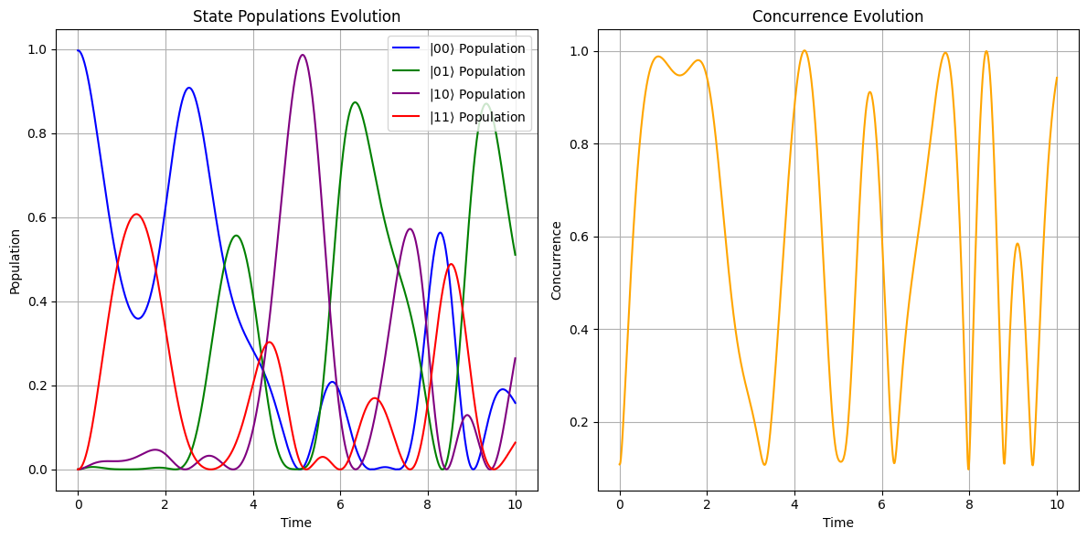
Figure 2: Coherent Dynamics and Entanglement in a Two-Qubit System. Left: Evolution of the populations for the basis states $|00\rangle$, $|01\rangle$, $|10\rangle$, and $|11\rangle$ of a two-qubit quantum system over time, illustrating the oscillatory behavior due to the system’s coherent dynamics. Each curve represents the population of a corresponding quantum state, indicating the transient dominance of certain states at various time intervals. Right: The concurrence evolution of the same system, demonstrating the periodic generation and annihilation of quantum entanglement. The concurrence oscillates between 0 (no entanglement) and values close to 1 (near-maximal entanglement), reflecting the impact of time-dependent control fields on the entanglement properties of the system.

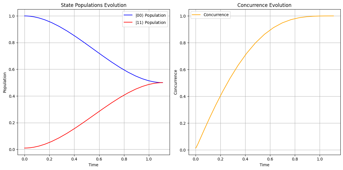
Figure 3: Evolution of Quantum State Populations and Entanglement via Optimal Control. Left: The graph demonstrates the time-dependent variation of the populations for the states $|00\rangle$ and $|11\rangle$, showing the transfer of population between these two states as a function of time. Right: The concurrence evolution exhibits a monotonic increase, signifying the enhancement of entanglement between the two qubits under the applied optimal control strategy. The concurrence approaches a plateau as the system reaches a near-maximally entangled state.

V Conclusion

In this paper, we have streamlined quantum optimal control for entangling bipartite systems, utilizing the indirect Pontryagin Minimum Principle to maximize an enhanced lower bound of entanglement. Our framework, empowered by a neural network approach, can efficiently produce entangled states. The insights gained lay the groundwork for advanced control in complex quantum systems and could greatly benefit the integration with current quantum technologies. This refined control mechanism promises significant strides in quantum networking and computing. Future work will extend these strategies to high-dimensional and multipartite systems, with considerations for dissipative effects and noise in realistic scenarios.

References

- [1] N. Zou, “Quantum entanglement and its application in quantum communication,” in Journal of Physics: Conference Series, vol. 1827, no. 1. IOP Publishing, 2021, p. 012120.
- [2] A. Datta and G. Vidal, “Role of entanglement and correlations in mixed-state quantum computation,” Physical Review A, vol. 75, no. 4, p. 042310, 2007.
- [3] M. Choi and S. Lee, “Quantum cryptographic resource distillation and entanglement,” Scientific Reports, vol. 11, no. 1, p. 21095, 2021.
- [4] Y. Liu, S. Kuang, and S. Cong, “Lyapunov-based feedback preparation of ghz entanglement of -qubit systems,” IEEE Transactions on Cybernetics, vol. 47, no. 11, pp. 3827–3839, 2016.
- [5] Z.-X. Ding, C.-S. Hu, L.-T. Shen, Z.-B. Yang, H. Wu, and S.-B. Zheng, “Dissipative entanglement preparation via rydberg antiblockade and lyapunov control,” Laser Physics Letters, vol. 16, no. 4, p. 045203, 2019.
- [6] K. Mishima and K. Yamashita, “Free-time and fixed end-point optimal control theory in quantum mechanics: Application to entanglement generation,” The Journal of chemical physics, vol. 130, no. 3, 2009.
- [7] F. Platzer, F. Mintert, and A. Buchleitner, “Optimal dynamical control of many-body entanglement,” Physical review letters, vol. 105, no. 2, p. 020501, 2010.
- [8] P. Poggi and D. A. Wisniacki, “Optimal control of many-body quantum dynamics: Chaos and complexity,” Physical Review A, vol. 94, no. 3, p. 033406, 2016.
- [9] D. Stefanatos, “Maximising optomechanical entanglement with optimal control,” Quantum Science and Technology, vol. 2, no. 1, p. 014003, 2017.
- [10] F. Albarelli, U. Shackerley-Bennett, and A. Serafini, “Locally optimal control of continuous-variable entanglement,” Physical Review A, vol. 98, no. 6, p. 062312, 2018.
- [11] X. Li, “Optimal control of quantum state preparation and entanglement creation in two-qubit quantum system with bounded amplitude,” Scientific Reports, vol. 13, no. 1, p. 14734, 2023.
- [12] M. J. Donald, M. Horodecki, and O. Rudolph, “The uniqueness theorem for entanglement measures,” Journal of Mathematical Physics, vol. 43, no. 9, pp. 4252–4272, 2002.
- [13] V. Vedral and M. B. Plenio, “Entanglement measures and purification procedures,” Physical Review A, vol. 57, no. 3, p. 1619, 1998.
- [14] G. Vidal, “Entanglement monotones,” Journal of Modern Optics, vol. 47, no. 2-3, pp. 355–376, 2000.
- [15] M. Horodecki, “Entanglement measures.” Quantum Inf. Comput., vol. 1, no. 1, pp. 3–26, 2001.
- [16] M. A. Nielsen and I. L. Chuang, Quantum computation and quantum information. Cambridge university press Cambridge, 2001, vol. 2.
- [17] V. S. Bhaskara and P. K. Panigrahi, “Generalized concurrence measure for faithful quantification of multiparticle pure state entanglement using lagrange’s identity and wedge product,” Quantum Information Processing, vol. 16, pp. 1–15, 2017.
- [18] S. J. Akhtarshenas, “Concurrence vectors in arbitrary multipartite quantum systems,” Journal of Physics A: Mathematical and General, vol. 38, no. 30, p. 6777, 2005.
- [19] M.-J. Zhao, X.-N. Zhu, S.-M. Fei, and X. Li-Jost, “Lower bound on concurrence and distillation for arbitrary-dimensional bipartite quantum states,” Physical Review A, vol. 84, no. 6, p. 062322, 2011.
- [20] Y.-C. Ou, H. Fan, and S.-M. Fei, “Proper monogamy inequality for arbitrary pure quantum states,” Physical Review A, vol. 78, no. 1, p. 012311, 2008.
- [21] K. Chen, S. Albeverio, and S.-M. Fei, “Concurrence of arbitrary dimensional bipartite quantum states,” Physical review letters, vol. 95, no. 4, p. 040504, 2005.
- [22] M. Horodecki, P. Horodecki, and R. Horodecki, “Mixed-state entanglement and distillation: Is there a “bound” entanglement in nature?” Physical Review Letters, vol. 80, no. 24, p. 5239, 1998.
- [23] K. Graichen, A. Kugi, N. Petit, and F. Chaplais, “Handling constraints in optimal control with saturation functions and system extension,” Systems & Control Letters, vol. 59, no. 11, pp. 671–679, 2010.
- [24] N. B. Dehaghani, A. P. Aguiar, and R. Wisniewski, “Quantum pontryagin neural networks in gamkrelidze form subjected to the purity of quantum channels,” IEEE Control Systems Letters, 2023.
- [25] A. D’ambrosio, E. Schiassi, F. Curti, and R. Furfaro, “Pontryagin neural networks with functional interpolation for optimal intercept problems,” Mathematics, vol. 9, no. 9, p. 996, 2021.