Optimization on a Finer Scale:
Bounded Local Subgradient Variation Perspective

Abstract

We initiate the study of nonsmooth optimization problems under bounded local subgradient variation, which postulates bounded difference between (sub)gradients in small local regions around points, in either average or maximum sense. The resulting class of objective functions encapsulates the classes of objective functions traditionally studied in the optimization literature, which are defined based on either Lipschitz continuity of the objective (in the case of nonsmooth optimization) or Hölder/Lipschitz continuity of the function’s gradient (in the case of weakly smooth/smooth optimization). Further, the defined class is richer in the sense that it contains functions that are neither Lipschitz continuous nor have a Hölder continuous gradient. Finally, when restricted to the aforementioned traditional classes of optimization problems, the constants defining the studied classes lead to more fine-grained complexity bounds, recovering traditional oracle complexity bounds in the worst case but generally leading to lower oracle complexity for functions that are not “worst case.” Some highlights of our results are that: (i) it is possible to obtain complexity results for both convex and nonconvex optimization problems with (local or global) Lipschitz constant being replaced by a constant of local subgradient variation, corresponding to small local regions and (ii) complexity of the subgradient set around the set of optima plays a role in the complexity of nonsmooth optimization, particularly in parallel optimization settings; in particular, functions with “simple” subgradient sets around optima can be optimized more efficiently, where simplicity is measured by the mean width of the function’s subdifferential set in a region around optima. A consequence of (ii) is that for any error parameter $\epsilon>0$, parallel oracle complexity of nonsmooth Lipschitz convex optimization is lower than its sequential oracle complexity by a factor $\tilde{\Omega}\big{(}\frac{1}{\epsilon}\big{)}$ whenever the objective function is a piecewise linear function with the number of pieces polynomial in the dimension and $1/\epsilon.$ This is particularly surprising considering that existing parallel complexity lower bounds are based on such classes of functions. The seeming contradiction is resolved by considering the region in which the algorithm is allowed to query the objective.

1 Introduction

Nonsmooth optimization problems pose some of the most intricate challenges within the realm of continuous optimization. As a result, they have been intensively studied from the algorithm design perspective since at least the 1960s [1, 33, 37]. The study of nonsmooth optimization concerns solving minimization problems of the form

$$\min_{\mathbf{x}\in\mathcal{X}}f(\mathbf{x}),$$ (P)

where $f$ is a (typically Lipschitz) continuous function (or satisfies other structural properties) and is not necessarily everywhere differentiable. Within this work, we are concerned with functions that are locally Lipschitz-continuous, in the sense that they have bounded Lipschitz constants on compact sets, but, importantly, we make no assumptions about the values of those Lipschitz constants. We further focus on standard settings where $\mathcal{X}$ is closed, convex, nonempty, and admits efficiently computable projections.

It was noted very early on that even though the objectives in such nonsmooth optimization problems are continuous (and, as such, differentiable almost everywhere, as a consequence of the classical Rademacher’s theorem [55]), traditional methods developed for smooth optimization generally fail to converge when applied to them as a black box. It was formally established in the subsequent literature that in terms of oracle-based worst-case complexity, (Lipschitz-continuous) nonsmooth optimization problems are more challenging than smooth optimization problems, both in the settings of convex [47] and nonconvex [35] optimization, unless additional assumptions about the structure [9, 49] and/or oracle access to $f$ [27, 31, 9, 42, 41, 57] are made and crucially used in the algorithm design and analysis.

Despite the computational barriers preventing further algorithmic speedups of nonsmooth optimization in the worst case, common nonsmooth optimization problems are often shown to be solvable with faster converging algorithms (even without access to stronger oracles such as the proximal oracle), sometimes even exhibiting linear (i.e., with geometrically reducing error) convergence locally and/or in practice [16, 32]. This large gap between the worst-case lower bounds and empirical performance on common instances prompts the question:

What type of structure makes certain nonsmooth optimization problems easier than others, and what kind of algorithms effectively exploit such structural properties?

1.1 Motivation & Intuition

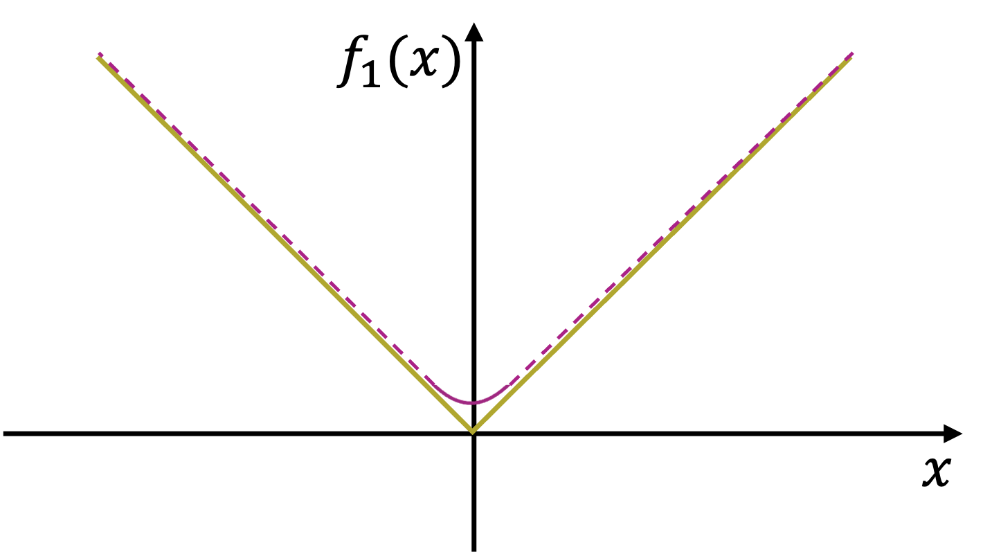
(a) “farther from smooth”

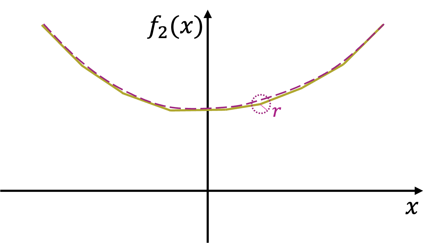
(b) “closer to smooth”

Figure 1: Two nonsmooth, piecewise-linear, functions with the same Lipschitz constant. If both functions are averaged over a radius $r$ shown on the right plot, the right function remains much closer to its averaged, smoothed, variant indicated by the dashed line. Further, on any local neighborhood of radius $r$, the right function exhibits much milder changes in the slope than the left function does on its (only) kink.

Our starting point for the research presented in this work came from observations illustrated in Figure 1, which depicts two nonsmooth, Lipschitz-continuous, piecewise-linear functions that both have the same Lipschitz constant. Visually, it is apparent that the right function is closer to a smooth function than the left function, in the sense that averaging both functions over small intervals around each point to obtain their smoothed counterparts, the right function remains much closer to its smoothing than the left one, in the sense of the maximum deviation. Thus, intuitively, the right function should be easier to optimize, as the oracle complexity of smooth optimization is lower than the oracle complexity of nonsmooth optimization. However, to the best of our knowledge, this is not captured by existing results.

Taking a closer look at the examples in Figure 1, we can notice that the property that differentiates these two functions and makes one closer to its smooth approximation than the other is how much the slope of the function varies across small regions. This basic observation is the main motivation for introducing the notions of local subgradient variation – corresponding to variation on average and in the worst-case, maximum sense – and studying oracle complexity of nonsmooth optimization under these notions of subgradient variation.

Our work is importantly motivated by the limitations encountered in the extensively studied technique of randomized smoothing (see e.g., [21, 51]), that uses convolution with a (uniform over a ball or Gaussian) kernel to reduce a nonsmooth (deterministic) optimization problem into a stochastic smooth optimization one, or even a problem only requiring access to a stochastic zeroth-order oracle. It is a well-known fact that in this setting oracle complexity necessarily scales polynomially with the dimension [51, 21, 35, 19, 43], which severely limits its applicability in high-dimensional problems. As another notion of fine-grained complexity, we demonstrate in this work that it is the complexity of the subgradient around a function minimizer $\mathbf{x}_{*}$ (assumed to exist in this work) that determines whether this dependence on the dimension can be improved. In particular, for a “simple” subgradient set around $\mathbf{x}_{*}$, the dependence on the dimension $d$ can be brought down to $\sqrt{\ln(d)}$ or even constant. This is further discussed in the next subsection and in Section 4.1.3.

Before moving onto describing our main results, we highlight the following properties of the functions that have bounded local variation of the subgradient (a more precise discussion is provided in Section 3, where these notions are formally introduced). First, every Lipschitz function has bounded local variation of the subgradient (under any of the considered average/maximum criteria), with the constant of subgradient variation being larger than the Lipschitz constant by at most a factor of 2, but possibly being arbitrarily smaller. In particular, the converse to this statement is not true: there are functions that have bounded local subgradient variation but are not Lipschitz-continuous (see Example 3.10 in Section 3.3). Thus, the class of functions with bounded local subgradient variation strictly contains the class of Lipschitz-continuous functions. Second, bounded local subgradient variation does not preclude superlinear (including quadratic) growth of a function, which clearly is not true for functions that are only Lipschitz continuous. Finally, we note that while the notion of subgradient variation is not new and it has been explored at least in the maximum and global sense [48, 50, 17], the key insight of our work is that it suffices for such a property to hold only in a local sense, between points sufficiently close to each other.

1.2 Main Results

Our main findings are summarized as follows.

Local subgradient variation as a measure of complexity.

The main contribution of this work is introducing and initiating the study of new classes of objectives in the context of (convex and nonconvex) nonsmooth optimization. These classes of objectives are called bounded maximum local variation of subgradients (or Grad-BMV, for short) and bounded mean local oscillation of subgradients (or Grad-BMO, for short), and are introduced in Section 3. Grad-BMO is the weaker of these two properties, in the sense that it is implied by Grad-BMV, while the converse does not hold in general. We provide different characterizations of structural properties of functions under these two notions of local subgradient variation and systematically investigate the complexity of classes of Grad-BMV and Grad-BMO problems, with the focus on demonstrating that these weak regularity properties suffice for obtaining a more fine-grained characterization of oracle complexity. Notably, because Grad-BMV and Grad-BMO functions are not necessarily (globally) Lipschitz continuous (but all Lipschitz-continuous functions are both Grad-BMV and Grad-BMO with a constant at most 2 times larger and possibly much smaller), on a conceptual level, our results demonstrate that weaker properties than Lipschitz continuity suffice for tractability of optimization in the oracle complexity model of computation.

Deterministic convex optimization under Grad-BMV.

We begin our discussion of oracle upper bounds under bounded local subgradient variation by treating Grad-BMV functions as approximately smooth functions. While this idea is not new and was used in [17, 50] as a means of handling weakly smooth functions in a universal manner, the prior work has only considered the settings in which such properties hold in a global sense, between any pair of points. By contrast, we demonstrate that only a local such property, assumed to hold only between points at distance at most $r>0$, suffices. As a result, we obtain results that are similar to those in [17, 50], but with a parameter that is potentially much lower than the Lipschitz/weak smoothness constants from prior work (recall the examples from Figure 1 and note also that Grad-BMV constant can be finite even in some cases where the global Lipschitz constant cannot be bounded above), thus providing a more fine-grained characterization of oracle complexity.

Randomized and possibly parallel convex optimization under Grad-BMV and Grad-BMO.

As mentioned before, one of our main initial goals in this work was to understand and possibly remove the computational barriers of randomized smoothing, which introduces polynomial dependence on the dimension in the oracle complexity bound. If one further considers parallel settings, where $\mathrm{poly}(d,1/\epsilon)$ queries may be asked in parallel per round of computation, then the term with the polynomial dependence on the dimension dominates the complexity (measured as the number of sequential rounds of queries), and this polynomial dependence is unavoidable in the worst case [19, 2, 6, 63, 43]. As another measure of fine-grained complexity, we show that this worst-case polynomial dependence on the dimension is determined by the complexity of the subgradient around a minimizer $\mathbf{x}_{*}\in\operatorname{\mathrm{argmin}}_{\mathbf{x}}f(\mathbf{x}).$ In particular, let $\partial f_{r}(\mathbf{x}_{*})$ be the convex hull of the subgradients in the Euclidean ball of radius $r=O(\epsilon\sqrt{d})$, centered at $\mathbf{x}_{*}.$ The diameter of this set is determined by the Grad-BMV constant, denoted by $\widehat{L}_{r}.$ Let $K_{\mathbf{x}_{*}}$ be the polytope of diameter $O(\widehat{L}_{r})$ that contains $\partial f_{r}(\mathbf{x}_{*})$ and has the smallest number of vertices. Then, the dimension-dependent term in the oracle complexity can be bounded by $O(\sqrt{\ln(\operatorname{vert}(K_{\mathbf{x}_{*}}))}),$ where $\operatorname{vert}(K_{\mathbf{x}_{*}})$ denotes the number of vertices of $K_{\mathbf{x}_{*}}.$ As a result, when $\operatorname{vert}(K_{\mathbf{x}_{*}})=O(\mathrm{poly}(d)),$ the dependence on the dimension can be brought down to at most $O(\sqrt{\ln(d)}),$ which is nearly dimension-independent. Note that this result does not contradict prior lower bounds for parallel convex optimization [19, 2, 6, 63], as is explained in Section 4.1.3.

Nonconvex optimization under Grad-BMV.

Our final set of results concerns nonconvex nonsmooth optimization. We build on recent results for Goldstein’s method [15, 65] and show that the local Lipschitz constant used in the past work can be replaced by the generally much smaller local constant of Grad-BMV. In obtaining this result, we generalize and further simplify the analysis from [15].

1.3 Related Work

The complexity of continuous optimization is an actively investigated problem since the 1970s [46]. One of the main achievements of this theory is the precise quantification of the minimax optimal rates of convergence for smooth vs. nonsmooth convex optimization. However, as we argued earlier, this coarse parameterization based on the maximum Lipschitz constant (either for the objective or its gradient) misses much of the information that determines the difficulty of performing optimization. The goal of our work is to bridge this gap. Below we review various threads of research that are related to our work.

Smoothing approaches.

Both randomized and deterministic smoothing approaches have been widely used in nonlinear optimization for a long time and in different contexts [60, 4, 53, 52, 64, 36, 21, 6, 22, 46, 49, 51]. Some of the most basic examples are the use of Moreau envelope for deterministic methods (see, e.g., [42, 57]), which requires access to a proximal point oracle, and local randomized smoothing using a Gaussian kernel or uniform distribution on a ball or a sphere [60, 46, 22, 51, 21] (all these kernels lead to very similar results, due to concentration properties of these distributions in high dimensions; see, e.g., [5, Chapter 2]). The idea of smoothing is a natural one: approximate a nonsmooth function by a smooth one and then apply methods for smooth minimization to the smoothed function. We note that the goal of our work is not to devise new smoothing approaches (in fact, we rely on a very simple randomized smoothing over a Euclidean ball), but to demonstrate usefulness of the introduced Grad-BMO concept in proving oracle complexity upper bounds.

Local Lipschitzness and Relaxations.

Much of the recent literature on nonsmooth optimization (e.g., [16, 15]) replaces the global Lipschitz condition by a local one, which posits Lipschitz continuity on compact sets and implies bounded subgradients on those sets. This is based on the insight that many optimization algorithms ensure that their iterates remain on a compact set around optima, thus how function behaves outside this set is irrelevant for optimization. An alternative definition is that of Lipschitz continuity in local neighborhoods of points (see [13, Chapter 1]); however, this definition seems to have been primarily used to define and study generalized notions of derivatives rather than oracle complexity of optimization. We further highlight the following works which addressed nonsmooth problems that are not necessarily Lipschitz-continuous. In [26], a variant of projected subgradient method with normalized subgradients was analyzed, motivated by insights from [58]. This work shows that the rate of convergence $1/\sqrt{k}$ can be established assuming that there is a nondecreasing nonnegative mapping $\mathcal{D}:\mathbb{R}_{+}\to\mathbb{R}_{+}\cup\{+\infty\}$ such that $f(\mathbf{x})-f(\mathbf{x}_{*})\leq\mathcal{D}(\|\mathbf{x}-\mathbf{x}_{*}\|_{2})$ where $\mathbf{x}_{*}$ is a fixed minimizer of $f$ and the complexity results are expressed in terms of this mapping. Such an assumption removes the requirement for regularity such as Lipschitz continuity to hold on a compact set between any pair of points, but still requires at least some bounded growth condition to hold on the entire feasible set or on a sufficiently large ball around $\mathbf{x}_{*}$. Another line of work [56, 25] develops a generic transformation from nonsmooth non-Lipschitz convex problems to convex Lipschitz problems and an algorithmic framework to address them at the cost of a simple line search (but removing projections in constrained settings) and with an error guarantee of the form $\frac{f(\mathbf{x})-f(\mathbf{x}_{*})}{f(\mathbf{x}_{0})+c-f(\mathbf{x}_{*})}\leq\epsilon,$ where $c>0$ is a parameter of the algorithm. This corresponds to a multiplicative error guarantee for the shifted function $f(\cdot)-f(\mathbf{x}_{0})-c,$ but on the original problem the error additive and equal to $(f(\mathbf{x}_{0})-f(\mathbf{x}_{*})+c)\epsilon.$ The resulting complexity bound replaces the usual dependence on the Lipschitz constant in traditional oracle complexity bounds for Lipschitz convex optimization by the inverse of a parameter defined by $R=\sup\{r\in\mathbb{R}:f(\mathbf{x})\leq f(\mathbf{x}_{0})+c\text{ for all }\mathbf{x}\text{ with }\|\mathbf{x}-\mathbf{x}_{0}\|_{2}\leq r\}$. Given a fixed $c,$ for Lipschitz functions this constant is bounded by $c/M$, where $M$ is the Lipschitz constant of $f$ on the sublevel set $\{\mathbf{x}:f(\mathbf{x})\leq f(\mathbf{x}_{0})+c\}.$ More generally, for the result to be informative, one needs to bound the growth of $f$ on a sufficiently large neighborhood of $\mathbf{x}_{0}$ intersected with the sublevel set $\{\mathbf{x}:f(\mathbf{x})\leq f(\mathbf{x}_{0})+c\}.$ In summary, all the results using notions of local Lipschitzness (and related concepts) that we are aware of require bounding the growth of the function in a possibly small region. By contrast, our results rely on bounding the subgradient variation in local regions.

Stronger oracles.

Improved complexity results for nonsmooth optimization are possible if access to additional oracles or structure of the problem is accessible to the algorithm. For example, there is vast literature on methods utilizing the proximal point oracle (see, e.g., [57, 28, 29, 11]), requiring oracle access to minima of problems of the form $f(\mathbf{x})+\frac{1}{2\tau}\|\mathbf{x}-\mathbf{x}_{0}\|_{2}^{2}$ for any $\mathbf{x}_{0}\in\mathbb{R}^{d}$ and $\tau>0.$ Another example in the recent literature is the ball oracle [8], which gives the algorithm access to solutions of the problem $\min_{\mathbf{x}:\|\mathbf{x}-\mathbf{x}_{0}\|_{2}\leq r}f(\mathbf{x})$ for any $\mathbf{x}_{0}\in\mathbb{R}^{d}$ and some $r>0.$ Further, there are multiple results assuming that the objective function can be expressed as a structured maximization problem (e.g., arising from the convex conjugate of a function $f$ composed with a linear map $\mathbf{A}\mathbf{x}$ [49, 11] or the objective simply being a maximum of $N$ smooth or nonsmooth functions [9]) and where one is given oracle access to components of the said maximization problem (such as proximal point oracle access to the convex conjugate of $F$ in the case of $f(\mathbf{x})=F(\mathbf{A}\mathbf{x})$ or first-order oracle access to component functions in the case where $f(\mathbf{x})=\max_{1\leq i\leq n}f_{i}(\mathbf{x})$). Finally, it is possible to relax Lipschitz continuity by “relative continuity” – where $\|\nabla f(\mathbf{x})\|_{*}\leq\frac{\sqrt{2MD_{h}(\mathbf{y},\mathbf{x})}}{\|\mathbf{y}-\mathbf{x}\|}$ for a pair of dual norms $\|\cdot\|,\|\cdot\|_{*},$ a positive constant $M$, and Bregman divergence $D_{h}$ w.r.t. a reference function $h$ – and recover the complexity results of nonsmooth Lipschitz convex optimization [39]. However, this approach requires oracle access to minimizers of $D_{h}(\mathbf{x},\mathbf{x}_{0})+\left\langle\mathbf{z},\mathbf{x}\right\rangle$ for arbitrary but fixed $\mathbf{x}_{0},\mathbf{z}$, which correspond to mirror descent steps, and, moreover, there are few examples of functions that satisfy such a relative continuity property. Our work does not require any specialized oracles but only relies on the standard first-order oracle.

Finally, our work leverages existing algorithms and techniques in convex [12, 23, 50] and nonconvex optimization [65, 15]. We note here that our focus is not on algorithm design but on novel characterizations of oracle complexity in optimization. In particular, we demonstrate that existing algorithms can be analyzed for the complexity classes based on bounded local subgradient variation that we introduce and oracle complexity results that are both more general and more fine-grained can be obtained.

2 Preliminaries

Our primary focus is on the Euclidean space $(\mathbb{R}^{d},\|\cdot\|_{2})$; however, much of the discussion extends to other normed spaces. We use $\mathcal{B}:=\{\mathbf{x}\in\mathbb{R}^{d}:\|\mathbf{x}\|_{2}\leq 1\}$ to denote the centered unit Euclidean ball and $\mathcal{B}_{r}(\bar{\mathbf{x}}):=\{\mathbf{x}\in\mathbb{R}^{d}:\|\mathbf{x}-\bar{\mathbf{x}}\|_{2}\leq r\}$ to denote the Euclidean ball of radius $r$ centered at $\bar{\mathbf{x}}$. When $\bar{\mathbf{x}}=0$, we use the notation $\mathcal{B}_{r}:=\mathcal{B}_{r}(0)$. We use $\mathcal{S}:=\{\mathbf{x}\in\mathbb{R}^{d}:\|\mathbf{x}\|_{2}=1\}$ to denote the centered unit sphere w.r.t. the Euclidean norm.

We say that a function $f:\mathbb{R}^{d}\to\mathbb{R}$ is $M$-Lipschitz continuous for some constant $M<\infty,$ if for any $\mathbf{x},\mathbf{y}\in\mathbb{R}^{d},$

$$|f(\mathbf{x})-f(\mathbf{y})|\leq M\|\mathbf{x}-\mathbf{y}\|_{2}.$$ (2.1)

If $f$ is additionally convex, then it is subdifferentiable on its whole domain; in particular $\partial f(\mathbf{x})\neq\emptyset$, for all $\mathbf{x}\in\mathbb{R}^{d}$. In such a case, we will denote for convenience by $\gamma_{f}(\mathbf{x})$ an arbitrary (measurable w.r.t. $\mathbf{x}$) selection from $\partial f(\mathbf{x})$. A similar conclusion holds without convexity (only under Lipschitzness), with the observation that here $f$ would be differentiable almost everywhere, thus a measurable selection would exist as well.

We say that a function $f:\mathbb{R}^{d}\to\mathbb{R}$ is locally Lipschitz if for every $r>0$, $f$ is Lipschitz over ${\cal B}_{r}$. Notice that we have made no assumptions about the Lipschitz constant on each of these balls: this is important as we would like to handle the case where the objective may not be globally Lipschitz with a uniform constant (e.g., a quadratic function). The main property of local Lipschitzness we need for our arguments is the almost sure differentiability of these functions, and the fundamental theorem of calculus. Both of them are stated below, for completeness.

Theorem 2.1 (Rademacher [55]).

If $f:\mathbb{R}^{d}\to\mathbb{R}$ is locally Lipschitz then it is differentiable almost everywhere.

Theorem 2.2 (Fundamental Theorem of Calculus (FTC)).

If $f:\mathbb{R}^{d}\to\mathbb{R}$ is locally Lipschitz, then for all $\mathbf{a},\mathbf{b}\in\mathbb{R}^{d}$

$$f(\mathbf{b})-f(\mathbf{a})=\int_{0}^{1}(\gamma_{f})_{\mathbf{a},\mathbf{b}}((1-t)\mathbf{a}+t\mathbf{b})\mathrm{d}t,$$

where $(\gamma_{f})_{\mathbf{a},\mathbf{b}}$ is a measurable selection of the directional derivative $f^{\prime}(\cdot;\mathbf{b}-\mathbf{a})$. Moreover, if either $\mathbf{a}$ or $\mathbf{b}$ are chosen generically,

$$f(\mathbf{b})-f(\mathbf{a})=\int_{0}^{1}\langle\gamma_{f}((1-t)\mathbf{a}+t\mathbf{b}),\mathbf{b}-\mathbf{a}\rangle\mathrm{d}t.$$

Finally, given $\delta>0$, we recall the definition of the Goldstein $\delta$-subdifferential of a (locally Lipschitz) function $f:\mathbb{R}^{d}\to\mathbb{R}$ at a point $\mathbf{x}\in\mathbb{R}^{d}$, $\partial_{\delta}f(\mathbf{x})=\mbox{conv}\Big{(}\bigcup_{\mathbf{y}\in{\cal B}(\mathbf{x},\delta)}\partial f(\mathbf{y})\Big{)}$. We say that a point $\mathbf{x}\in\mathbb{R}^{d}$ is $(\delta,\epsilon)$-stationary if $\mbox{dist}(0,\partial_{\delta}f(\mathbf{x}))\leq\epsilon$.

3 Bounded Local Variation of the Subgradient

In this section, we provide local regularity assumptions for the subgradient that define the complexity class that we study in this work. The two notions are: (i) bounded maximum local variation and (ii) bounded mean oscillation. We later argue that these two (local) assumptions are sufficient for obtaining upper complexity bounds. Both properties are defined for a fixed radius $r.$ We later discuss how this radius can be chosen or estimated. The motivation for the considered notions of local variability is illustrated in examples provided in Figure 1, as discussed in the introduction.

3.1 Bounded Maximum Local Variation

Bounded maximum local variation requires that the subgradient of a function does not change much over small regions, although it is possible for each of the subgradients to have a large norm. Formally,

Definition 3.1 (Bounded Maximum Local Variation).

Given $r>0,$ we say that a locally Lipschitz function $f:\mathbb{R}^{d}\to\mathbb{R}$ has bounded maximum local variation of the subgradient in norm $\|\cdot\|_{2},$ if there exists a positive constant $\widehat{L}_{r}<\infty$ such that for any $\mathbf{x}\in\mathbb{R}^{d}$ and any $\mathbf{u}\in\mathbb{R}^{d}$, $\|\mathbf{u}\|_{2}\leq 1$, it holds

$$\|\gamma_{f}(\mathbf{x}+r\mathbf{u})-\gamma_{f}(\mathbf{x})\|_{2}\leq\widehat{L}_{r}.$$

Observe that if $f$ were (globally) $L$-Lipschitz continuous, then $\widehat{L}_{r}\leq 2L.$ However, it is possible for $\widehat{L}_{r}$ to be much smaller than $L.$ For example, a univariate function $f$ equal to $\frac{1}{2}$ for $|x|<1$ and equal to $\frac{1}{2}x^{2}$ otherwise is clearly not Lipschitz continuous, but has bounded local variation of the (sub)gradient with $\widehat{L}_{r}=1$ for $r<2.$ (Observe that the “local” Lipschitz constant in the sense of [14, 16] would be much larger in general, as the derivative of $f$ scales with $x$ for $|x|>1,$ which is bounded on bounded sets, but scales with the diameter of the set.)

3.2 Bounded Mean Oscillation and Local Smoothing

Functions with Bounded Mean Oscillation (BMO functions) play an important role in harmonic analysis. They are formally defined as follows (see, e.g., [34]).

Definition 3.2 (Bounded Mean Oscillation).

Let $f:\mathbb{R}^{d}\to\mathbb{R}$ be a function that is integrable on compact sets. Then, $f$ is said to be a BMO function if

$$\|f\|_{\rm BMO}:=\sup_{\mathbf{x}\in\mathbb{R}^{d},r>0}\frac{1}{\operatorname{vol}(\mathcal{B}_{r})}\int_{\mathcal{B}_{r}}|f(\mathbf{x}+\mathbf{u})-f_{r}(\mathbf{x})|\mathrm{d}\mathbf{u}<\infty,$$ (3.1)

where $\operatorname{vol}$ denotes the volume and

$$f_{r}(\mathbf{x})=\frac{1}{\operatorname{vol}(\mathcal{B}_{r})}\int_{\mathcal{B}_{r}}f(\mathbf{x}+\mathbf{u})\mathrm{d}\mathbf{u}.$$ (3.2)

The (semi-)norm $\|\cdot\|_{\rm BMO}$ is referred to as the BMO norm.

We note that under minimal assumptions (e.g., local Lipschitzness), $f_{r}$ is differentiable. The integral $\frac{1}{\operatorname{vol}(\mathcal{B}_{r})}\int_{\mathcal{B}_{r}}|f(\mathbf{x}+\mathbf{u})-f_{r}(\mathbf{x})|\mathrm{d}\mathbf{u}$ is known as the mean oscillation of $f$ over $\mathcal{B}_{r}$. The above definition is often stated for the unit ball w.r.t. $\|\cdot\|=\|\cdot\|_{\infty},$ i.e., by defining BMO functions as functions with bounded oscillations $\frac{1}{\operatorname{vol}(\mathcal{B}_{r})}\int_{\mathcal{B}_{r}}|f(\mathbf{x}+\mathbf{u})-f_{r}(\mathbf{x})|\mathrm{d}\mathbf{u}$ over hypercubes. However, using the definition as ours is not uncommon in the literature and the definitions using different norms are all equivalent (though the value of the resulting BMO norms may differ) [62, 59]. In this work, we focus on the Euclidean case, where $\|\cdot\|=\|\cdot\|_{2}.$ All bounded functions are BMO.

Gradient BMO Functions

The definition of BMO functions is not directly useful in our setting, for two reasons: (1) the bounded oscillation is defined with respect to the function value, whereas in our case it is the slope (or the subgradient) whose changes with respect to small perturbations determine how close a function is to its smoothed approximation (see Figure 1); and (2) BMO is a global property of functions, whereas we are interested in small, local changes in the slope (or the subgradient). Accounting for these two issues, we introduce the following definition of (sub)gradient $r$-BMO functions.

Definition 3.3 (Bounded (Sub)Gradient Mean Oscillation).

Let $f:\mathbb{R}^{d}\to\mathbb{R}$ be a locally Lipschitz function. Given $r>0,$ we say that $f$ is (sub)gradient $r$-BMO if there exists $L_{r}<\infty$ such that

$$\|\nabla f\|_{{\rm BMO},r}:=\sup_{0<\rho\leq r}\sup_{\mathbf{x}\in\mathbb{R}^{d}}\frac{1}{\operatorname{vol}(\mathcal{S}_{\rho})}\int_{\mathcal{S}_{\rho}}\|\gamma_{f}(\mathbf{x}+\mathbf{u})-\nabla f_{r}(\mathbf{x})\|_{2}\mathrm{d}\mathbf{u}\leq L_{r},$$ (3.3)

where $f_{r}$ is defined by (3.2) and $\mathcal{S}_{\rho}=\{\mathbf{x}:\|\mathbf{x}\|_{2}=\rho\}$. In this case, we also say that $f$ is (sub)gradient $r$-BMO with constant $L_{r}.$ We say that $f$ is gradient BMO if

$$\|\nabla f\|_{{\rm BMO}}:=\sup_{r>0}\|\nabla f\|_{{\rm BMO},r}<\infty.$$

Gradient $r$-BMO property plays a role in local smoothing of a function. Intuitively, functions with lower gradient $r$-BMO constants are closer to their smooth approximations obtained using local smoothing (such as randomized smoothing over small balls used in this work). Our main insight is that this property, together with bounded maximum local variation from Definition 3.1, allows us to characterize complexity of nonsmooth optimization problem classes at a finer scale. For illustration, recall the two functions shown in Fig. 1. Both these functions are nonsmooth (in fact, both are piecewise-linear) with the same Lipschitz constant. However, the right function has a smaller gradient $r$-BMO constant $L_{r}$ for sufficiently small radius indicated on the right subfigure. Even though both functions belong to the same class of nonsmooth Lipschitz functions, visually, the right functions is “closer to being smooth,” as the transitions between the linear pieces have less dramatic changes in the slope.

Randomized Local Smoothing

Observe that, given $r>0$, if we consider the uniform distribution $\operatorname{Unif}(\mathcal{B}_{r})$ on the centered Euclidean ball of radius $r,$ $\mathcal{B}_{r}=r\mathcal{B},$ then we can equivalently define the smoothed function $f_{r}$ from (3.2) as

$$f_{r}(\mathbf{x}) =\mathbb{E}_{\mathbf{u}\sim\operatorname{Unif}(\mathcal{B}_{r})}[f(\mathbf{x}+\mathbf{u})]$$ (3.4)

$$=\mathbb{E}_{\mathbf{u}\sim\operatorname{Unif}(\mathcal{B})}[f(\mathbf{x}+r\mathbf{u})].$$

This observation gives rise to the use of randomized smoothing, where we can obtain an unbiased estimate of the (sub)gradient of $f_{r}$ using one of the two following ideas. The first is simply using $\gamma_{f}(\mathbf{x}+\mathbf{u})$, where $\mathbf{u}$ is drawn uniformly at random from $\mathcal{B}_{r}$: this results in an unbiased estimate by the dominated convergence theorem. The second is $f(\mathbf{x}+r\mathbf{u})\mathbf{u},$ where $\mathbf{u}$ is drawn uniformly at random from the sphere of radius one. This is a valid unbiased estimate as a consequence of Stokes theorem, summarized in the lemma below. The proof of the lemma can be found in [46, Chapter 9] and in [22], and is thus omitted for brevity.

Lemma 3.4.

Given $r>0,$

$$\mathbb{E}_{\mathbf{u}\sim\operatorname{Unif}(\mathcal{S})}[f(\mathbf{x}+r\mathbf{u})\mathbf{u}]=\frac{r}{d}\nabla f_{r}(\mathbf{x}).$$ (3.5)

We first show that for gradient $r$-BMO convex functions with small constant $L_{r}$, the smoothed function $f_{r}$ is close to the original function $f$, which aligns well with our intuition from the previous subsection.

Lemma 3.5.

Let $f:\mathbb{R}^{d}\to\mathbb{R}$ be a locally Lipschitz function that is subgradient $r$-BMO with constant $L_{r}$ and let $f_{r}$ be defined by (3.4). Then, for all $\mathbf{x}\in\mathbb{R}^{d},$

$$f_{r}(\mathbf{x})-f(\mathbf{x})\leq L_{r}r.$$

Additionally, if $f$ is convex, then $f_{r}(\mathbf{x})-f(\mathbf{x})\geq 0,$ $\forall\mathbf{x}\in\mathbb{R}^{d}.$

Proof.

The second claim (for convex functions) follows from Jensen’s inequality. For the first claim, we start by using the definition of $f_{r}$ and the fundamental theorem of calculus (see Theorem 2.2) applied to $f$ to conclude that

$$f_{r}(\mathbf{x})-f(\mathbf{x}) =\mathbb{E}_{\mathbf{u}\sim\operatorname{Unif}(\mathcal{B})}[f(\mathbf{x}+r\mathbf{u})-f(\mathbf{x})]$$

$$=\mathbb{E}_{\mathbf{u}\sim\operatorname{Unif}(\mathcal{B})}\bigg{[}\int_{0}^{1}\left\langle\gamma_{f}(\mathbf{x}+tr\mathbf{u}),r\mathbf{u}\right\rangle\mathrm{d}t\bigg{]}.$$

Because $\operatorname{Unif}(\mathcal{B}_{r})$ is centrally symmetric, we have that $\mathbb{E}_{\mathbf{u}\in\operatorname{Unif}(\mathcal{B})}[\left\langle\mathbf{z},\mathbf{u}\right\rangle]=0$ for any fixed vector $\mathbf{z}\in\mathbb{R}^{d}$. Hence, $\mathbb{E}_{\mathbf{u}\in\operatorname{Unif}(\mathcal{B})}[\left\langle\nabla f_{r}(\mathbf{x}),\mathbf{u}\right\rangle]=0$ and thus we can write

$$|f_{r}(\mathbf{x})-f(\mathbf{x})| =r\bigg{|}\mathbb{E}_{\mathbf{u}\sim\operatorname{Unif}(\mathcal{B})}\bigg{[}\int_{0}^{1}\left\langle\gamma_{f}(\mathbf{x}+tr\mathbf{u})-\nabla f_{r}(\mathbf{x}),\mathbf{u}\right\rangle\mathrm{d}t\bigg{]}\bigg{|}$$

$$\stackrel{{\scriptstyle(i)}}{{\leq}}r\mathbb{E}_{\mathbf{u}\sim\operatorname{Unif}(\mathcal{B})}\bigg{[}\int_{0}^{1}\|\gamma_{f}(\mathbf{x}+tr\mathbf{u})-\nabla f_{r}(\mathbf{x})\|_{2}\|\mathbf{u}\|_{2}\mathrm{d}t\bigg{]}$$

$$\stackrel{{\scriptstyle(ii)}}{{\leq}}r\mathbb{E}_{\mathbf{u}\sim\operatorname{Unif}(\mathcal{B})}\bigg{[}\int_{0}^{1}\|\gamma_{f}(\mathbf{x}+tr\mathbf{u})-\nabla f_{r}(\mathbf{x})\|_{2}\mathrm{d}t\bigg{]}$$

$$\stackrel{{\scriptstyle(iii)}}{{=}}r\int_{0}^{1}\mathbb{E}_{\mathbf{u}\sim\operatorname{Unif}(\mathcal{B})}\big{[}\|\gamma_{f}(\mathbf{x}+tr\mathbf{u})-\nabla f_{r}(\mathbf{x})\|_{2}\big{]}\mathrm{d}t$$

$$\stackrel{{\scriptstyle(iv)}}{{\leq}}rL_{r},$$

where (i) is by Jensen’s inequality and Cauchy-Schwarz, (ii) is by the fact that the norm of the vector $\mathbf{u}\in\mathcal{B}$ is uniformly bounded by $1,$ (iii) is by Fubini’s theorem, and (iv) follows from Definition 3.3. ∎

It is possible to obtain a tighter bound on the distance between $f$ and $f_{r}$ under an additional assumption about the subgradients of $f.$ This result is summarized in the following lemma and it will be particularly useful for obtaining near-dimension-independent convergence results in the parallel optimization setting.

Lemma 3.6.

Let $f$ be a locally Lipschitz function. Then for almost all $\mathbf{x}\in\mathbb{R}^{d}$

$$f_{r}(\mathbf{x})-f(\mathbf{x})\leq r\,w(\partial_{r}f(\mathbf{x})),$$

where $w(K)=\mathbb{E}_{\mathbf{u}\sim\operatorname{Unif}{({\cal S})}}[\sup_{\mathbf{x}_{1},\mathbf{x}_{2}\in K}\langle\mathbf{u},\mathbf{x}_{1}-\mathbf{x}_{2}\rangle]$ denotes the mean width of $K$.

Proof.

For a generic $\mathbf{x}\in\mathbb{R}^{d}$, we have that $f$ is differentiable at $\mathbf{x}$. Hence, using the FTC and the central symmetry of $\mathcal{B}_{r}$, we have

$$f_{r}(\mathbf{x})-f(\mathbf{x}) =\mathbb{E}_{\mathbf{u}\sim\operatorname{Unif}(\mathcal{B}_{r})}[f(\mathbf{x}+\mathbf{u})-f(\mathbf{x})]$$

$$=\mathbb{E}_{\mathbf{u}\sim\operatorname{Unif}(\mathcal{B}_{r})}\bigg{[}\int_{0}^{1}\left\langle\gamma_{f}(\mathbf{x}+t\mathbf{u}),\mathbf{u}\right\rangle\mathrm{d}t\bigg{]}$$

$$=\mathbb{E}_{\mathbf{u}\sim\operatorname{Unif}(\mathcal{B}_{r})}\bigg{[}\int_{0}^{1}\left\langle\gamma_{f}(\mathbf{x}+t\mathbf{u})-\gamma_{f}(\mathbf{x}),\mathbf{u}\right\rangle\mathrm{d}t\bigg{]}.$$

Thus, letting $K=\partial_{r}f(\mathbf{x})$ we can further conclude that

$$f_{r}(\mathbf{x})-f(\mathbf{x}) \leq\mathbb{E}_{\mathbf{u}\sim\operatorname{Unif}(\mathcal{B}_{r})}\bigg{[}\int_{0}^{1}\sup_{\mathbf{g}_{1},\mathbf{g}_{2}\in K}\left\langle\mathbf{g}_{1}-\mathbf{g}_{2},\mathbf{u}\right\rangle\mathrm{d}t\bigg{]}$$

$$=r\mathbb{E}_{\mathbf{u}\sim\operatorname{Unif}(\mathcal{B})}\Big{[}\sup_{\mathbf{g}_{1},\mathbf{g}_{2}\in K}\left\langle\mathbf{g}_{1}-\mathbf{g}_{2},\mathbf{u}\right\rangle\Big{]}\mathrm{d}t$$ (3.6)

$$=rd\int_{0}^{1}\mathbb{E}_{\mathbf{u}\sim\operatorname{Unif}({\cal S})}\Big{[}\sup_{\mathbf{g}_{1},\mathbf{g}_{2}\in K}\left\langle\mathbf{g}_{1}-\mathbf{g}_{2},\tau\mathbf{u}\right\rangle\Big{]}\tau^{d-1}d\tau$$ (3.7)

$$=rw(K)d\int_{0}^{1}\tau^{d}d\tau$$

$$=\frac{d}{d+1}rw(K),$$

where in (3.7) we used integration by polar coordinates. ∎

Remark 3.7.

For discussions on the mean width, and the closely related Gaussian width, we refer the interested reader to [61, Section 7.5]. We provide some useful examples of mean width bounds from this reference:

1. Euclidean ball: $w(\mathcal{B})=1$.

2. Cube: $w([-1,+1]^{d})=\Theta(\sqrt{d})$.

3. Polytopes: If $K$ is a polytope with at most $k$ vertices, then $w(K)=O\Big{(}\mbox{diam}(K)\sqrt{\frac{\log(k)}{d}}\Big{)}$.

We note that the last example is particularly important. Many problems of interest in convex optimization can be formulated as (or approximated by) the maximum of finitely-many affine functions. In that case, the $1/\sqrt{d}$ factor that arises in the mean width bound provides a much more benign approximation than the worst-case bound for Lipschitz functions, corresponding to example (i).

We now argue about the smoothness of the function $f_{r}$ obtained via randomized smoothing.

Lemma 3.8.

Let $f:\mathbb{R}^{d}\to\mathbb{R}$ be a Grad-BMV function with constant $\widehat{L}_{r}$ and Grad-BMO with constant $L_{r},$ where both constants are defined w.r.t. the same fixed radius $r>0.$ Let $f_{r}$ be defined by (3.2). Then, for all $\mathbf{x},\mathbf{y}\in\mathbb{R}^{d},$

$$\|\nabla f_{r}(\mathbf{x})-\nabla f_{r}(\mathbf{y})\|_{2}\leq\min\Big{\{}\frac{L_{r}d}{r},\,O\Big{(}\frac{\widehat{L}_{r}\sqrt{d}}{r}\Big{)}\Big{\}}\|\mathbf{x}-\mathbf{y}\|_{2},$$

where $O(\cdot)$ only hides an absolute constant.

Proof.

For the first bound in the min, we use the characterization of $\nabla f_{r}$ from Lemma 3.4, as follows.

$$\|\nabla f_{r}(\mathbf{x})-\nabla f_{r}(\mathbf{y})\|_{2} =\frac{d}{r}\big{\|}\mathbb{E}_{\mathbf{u}\sim\operatorname{Unif}(\mathcal{S})}\big{[}\big{(}f(\mathbf{x}+r\mathbf{u})-f(\mathbf{y}+r\mathbf{u})\big{)}\mathbf{u}\big{]}\big{\|}_{2}$$

$$=\frac{d}{r}\bigg{\|}\mathbb{E}_{\mathbf{u}\sim\operatorname{Unif}(\mathcal{S})}\bigg{[}\int_{0}^{1}\left\langle\gamma_{f}(\mathbf{x}+r\mathbf{u}+t(\mathbf{y}-\mathbf{x})),\mathbf{y}-\mathbf{x}\right\rangle\mathrm{d}t\mathbf{u}\bigg{]}\bigg{\|}_{2},$$

where we have used the FTC. Because $\mathbf{u}$ is centrally symmetric, $\mathbb{E}_{\mathbf{u}\sim\operatorname{Unif}(\mathcal{S})}[c\mathbf{u}]=\textbf{0},$ for any constant $c.$ Hence, we can further write

$$\|\nabla f_{r}(\mathbf{x}) -\nabla f_{r}(\mathbf{y})\|_{2}$$

$$=\frac{d}{r}\bigg{\|}\mathbb{E}_{\mathbf{u}\sim\operatorname{Unif}(\mathcal{S})}\bigg{[}\int_{0}^{1}\left\langle\gamma_{f}(\mathbf{x}+r\mathbf{u}+t(\mathbf{y}-\mathbf{x}))-\nabla f_{r}(\mathbf{x}+t(\mathbf{y}-\mathbf{x})),\mathbf{y}-\mathbf{x}\right\rangle\mathrm{d}t\mathbf{u}\bigg{]}\bigg{\|}_{2}$$

$$\leq\frac{d}{r}\mathbb{E}_{\mathbf{u}\sim\operatorname{Unif}(\mathcal{S})}\bigg{[}\bigg{\|}\int_{0}^{1}\left\langle\gamma_{f}(\mathbf{x}+r\mathbf{u}+t(\mathbf{y}-\mathbf{x}))-\nabla f_{r}(\mathbf{x}+t(\mathbf{y}-\mathbf{x})),\mathbf{y}-\mathbf{x}\right\rangle\mathrm{d}t\mathbf{u}\bigg{\|}_{2}\bigg{]}$$

$$\leq\frac{d}{r}\mathbb{E}_{\mathbf{u}\sim\operatorname{Unif}(\mathcal{S})}\bigg{[}\int_{0}^{1}|\left\langle\gamma_{f}(\mathbf{x}+r\mathbf{u}+t(\mathbf{y}-\mathbf{x}))-\nabla f_{r}(\mathbf{x}+t(\mathbf{y}-\mathbf{x})),\mathbf{y}-\mathbf{x}\right\rangle|\mathrm{d}t\|\mathbf{u}\|_{2}\bigg{]}$$

$$\leq\frac{d}{r}\mathbb{E}_{\mathbf{u}\sim\operatorname{Unif}(\mathcal{S})}\bigg{[}\int_{0}^{1}\|\gamma_{f}(\mathbf{x}+r\mathbf{u}+t(\mathbf{y}-\mathbf{x}))-\nabla f_{r}(\mathbf{x}+t(\mathbf{y}-\mathbf{x}))\|_{2}\|\mathbf{y}-\mathbf{x}\|_{2}\mathrm{d}t\bigg{]}$$

$$=\frac{d\|\mathbf{y}-\mathbf{x}\|_{2}}{r}\mathbb{E}_{\mathbf{u}\sim\operatorname{Unif}(\mathcal{S})}\bigg{[}\int_{0}^{1}\|\gamma_{f}(\mathbf{x}+r\mathbf{u}+t(\mathbf{y}-\mathbf{x}))-\nabla f_{r}(\mathbf{x}+t(\mathbf{y}-\mathbf{x})))\|_{2}\mathrm{d}t\bigg{]}$$

$$\leq\frac{L_{r}d\|\mathbf{y}-\mathbf{x}\|_{2}}{r},$$

where we have used Jensen’s inequality (twice), $\|\mathbf{u}\|_{2}=1$ for $\mathbf{u}\in\mathcal{S}$, Cauchy-Schwarz inequality, and Definition 3.3.

For the second bound, we use the following sequence of inequalities:

$$\|\nabla f_{r}(x)-\nabla f_{r}(y)\|_{2}$$

$$=\; \frac{d}{r}\Big{\|}\mathbb{E}_{\mathbf{u}\sim\operatorname{Unif}(\mathcal{S})}[(f(\mathbf{x}+r\mathbf{u})-f(\mathbf{y}+r\mathbf{u}))\mathbf{u}]\Big{\|}_{2}$$

$$=\; \frac{d}{r}\sup_{\|\mathbf{v}\|_{2}\leq 1}\left\langle\mathbf{v},\mathbb{E}_{\mathbf{u}\sim\operatorname{Unif}(\mathcal{S})}[(f(\mathbf{x}+r\mathbf{u})-f(\mathbf{y}+r\mathbf{u}))\mathbf{u}]\right\rangle$$

$$=\; \frac{d}{r}\sup_{\|\mathbf{v}\|_{2}\leq 1}\left\langle\mathbf{v},\mathbb{E}_{\mathbf{u}\sim\operatorname{Unif}(\mathcal{S})}\bigg{[}\int_{0}^{1}\left\langle\gamma_{f}(\mathbf{x}+r\mathbf{u}+t(\mathbf{y}-\mathbf{x})),\mathbf{y}-\mathbf{x}\right\rangle\mathrm{d}t\mathbf{u}\bigg{]}\right\rangle$$

$$=\; \frac{d}{r}\sup_{\|\mathbf{v}\|_{2}\leq 1}\left\langle\mathbf{v},\mathbb{E}_{\mathbf{u}\sim\operatorname{Unif}(\mathcal{S})}\bigg{[}\int_{0}^{1}\left\langle\gamma_{f}(\mathbf{x}+r\mathbf{u}+t(\mathbf{y}-\mathbf{x}))-\gamma_{f}(\mathbf{x}+t(\mathbf{y}-\mathbf{x}))),\mathbf{y}-\mathbf{x}\right\rangle\mathrm{d}t\mathbf{u}\bigg{]}\right\rangle$$

$$=\; \frac{d}{r}\sup_{\|\mathbf{v}\|_{2}\leq 1}\mathbb{E}_{\mathbf{u}\sim\operatorname{Unif}(\mathcal{S})}\bigg{[}\left\langle\mathbf{v},\mathbf{u}\right\rangle\int_{0}^{1}\left\langle\gamma_{f}(\mathbf{x}+r\mathbf{u}+t(\mathbf{y}-\mathbf{x}))-\gamma_{f}(\mathbf{x}+t(\mathbf{y}-\mathbf{x}))),\mathbf{y}-\mathbf{x}\right\rangle\mathrm{d}t\bigg{]}$$

$$\leq\; \frac{d}{r}\sup_{\|\mathbf{v}\|_{2}\leq 1}\mathbb{E}_{\mathbf{u}\sim\operatorname{Unif}(\mathcal{S})}\big{[}|\left\langle\mathbf{v},\mathbf{u}\right\rangle|\big{]}\sup_{\|\mathbf{w}\|_{2}\leq 1}\bigg{|}\int_{0}^{1}\left\langle\gamma_{f}(\mathbf{x}+r\mathbf{w}+t(\mathbf{y}-\mathbf{x}))-\gamma_{f}(\mathbf{x}+t(\mathbf{y}-\mathbf{x}))),\mathbf{y}-\mathbf{x}\right\rangle\mathrm{d}t\bigg{|}$$

$$\leq\; \frac{\widehat{L}_{r}d}{r}\|\mathbf{y}-\mathbf{x}\|_{2}\sup_{\|\mathbf{v}\|_{2}\leq 1}\mathbb{E}_{\mathbf{u}\sim\operatorname{Unif}(\mathcal{S})}\big{[}|\left\langle\mathbf{v},\mathbf{u}\right\rangle|\big{]},$$

where we have used Definition 3.1 in the last inequality. To complete the proof, it remains to use

$$\sup_{\|\mathbf{v}\|_{2}\leq 1}\mathbb{E}_{\mathbf{u}\sim\operatorname{Unif}(\mathcal{S})}\big{[}|\left\langle\mathbf{v},\mathbf{u}\right\rangle|\big{]}=O\Big{(}\frac{1}{\sqrt{d}}\Big{)},$$

which follows from the concentration of measure on a (unit) sphere; see, for example, [3, Lemma 2.2]. ∎

3.3 A Discussion of Grad-BMV and Grad-BMO Classes

We now provide some examples that illustrate how classes of Grad-BMV and Grad-BMO functions compare to each other and to classical classes of objective functions studied in the optimization literature. First, based on the definition of constants $L_{r}$ and $\widehat{L}_{r}$ defining the Grad-BMO and Grad-BMV classes, it is immediate that

$$L_{r}\leq\widehat{L}_{r}.$$ (3.8)

As it turns out, it is possible for $L_{r}$ to be much smaller than $\widehat{L}_{r}.$ The overall intuition is that $L_{r}$ can be much smaller in cases where large local variation of the subgradient (which determines $\widehat{L}_{r}$) only happens on small subsets of the space, while in the rest of the space the variation is small. This is illustrated in the following example, where this intuitive observation is taken to the extreme to obtain simple expressions for the constants $L_{r}$ and $\widehat{L}_{r}$.

Example 3.9.

Consider the following function $f:\mathbb{R}^{d}\to\mathbb{R}$ for $c\in[1,\sqrt{d-1})$:

$$f(\mathbf{x})=\begin{cases}0,&\text{ if }|x_{1}|\leq\frac{c}{\sqrt{d-1}}\\ |x_{1}|-\frac{c}{\sqrt{d-1}},&\text{ if }|x_{1}|>\frac{c}{\sqrt{d-1}}\end{cases}.$$ (3.9)

This function is convex and 1-Lipschitz continuous. It is differentiable everywhere except at the set $\{|x_{1}|=\frac{c}{\sqrt{d-1}}\}$, with its subdifferential given by

$$\nabla f(\mathbf{x})=\begin{cases}\textbf{0},&\text{ if }|x_{1}|<\frac{c}{\sqrt{d-1}}\\ \mathrm{sign}(x_{1})\mathbf{e}_{1},&\text{ if }|x_{1}|>\frac{c}{\sqrt{d-1}}\\ \mathrm{conv}(\textbf{0},\mathrm{sign}(x_{1})\mathbf{e}_{1}),&\text{ if }|x_{1}|=\frac{c}{\sqrt{d-1}}\end{cases},$$ (3.10)

where $\mathrm{sign}(x_{1})$ is equal to one if $x_{1}>0$ and is equal to $-1$ otherwise, while $\mathbf{e}_{1}$ denotes the first standard basis vector. For $r\geq 2\frac{c}{\sqrt{d-1}},$ we have that $\widehat{L}_{r}=2$, which immediately follows from (3.10). On the other hand, the Grad-BMO constant $L_{r}$ is determined by the average gradient variation around $\mathbf{x}=\textbf{0},$ where, by symmetry, $\nabla f_{r}(\mathbf{x})=0.$ Assuming $\frac{c}{\sqrt{d-1}}\leq\frac{1}{2}$ and taking $r=1,$ we thus get that

$$L_{r}=\sup_{0<\rho\leq 1}\int_{\mathcal{S}_{\rho}}\|\gamma_{f}(\mathbf{x}+\mathbf{u})\|_{2}\mathrm{d}\mathbf{u}=\int_{\mathcal{S}_{1}}\|\gamma_{f}(\mathbf{x}+\mathbf{u})\|_{2}\mathrm{d}\mathbf{u}=\int_{\mathcal{S}_{1}\cap\{|x_{1}|>\frac{c}{\sqrt{d-1}}\}}1\mathrm{d}\mathbf{u}.$$

Using an adaption of [5, Theorem 2.7] from unit ball to unit sphere, it is possible to show that the above integral is bounded by $\frac{2}{c}e^{-c^{2}/2}.$ Thus, taking, e.g., $c=\frac{\sqrt{d-1}}{2}$ and increasing the dimension $d,$ we can make $L_{r}$ arbitrarily small.

Because $M$-Lipschitz continuous functions can be equivalently defined as functions whose subgradient is uniformly bounded by $M,$ it is immediate that $L_{r}\leq\widehat{L}_{r}\leq 2M$ for any $r>0.$ The latter inequality is tight in general, as is apparent by considering the univariate function $f(x)=M|x|.$

Classes of $(M,\kappa)$-weakly smooth functions for $\kappa\in[0,1]$ are also captured by classes of Grad-BMV and Grad-BMO functions. In particular, $(M,\kappa)$-weakly smooth functions are defined as continuously differentiable functions with Hölder-continuous gradient, in the sense that

$$\|\nabla f(\mathbf{x})-\nabla f(\mathbf{y})\|_{2}\leq M\|\mathbf{x}-\mathbf{y}\|_{2}^{\kappa},\quad\forall\mathbf{x},\mathbf{y}\in\mathbb{R}^{d}.$$ (3.11)

It is immediate from this definition that $L_{r}\leq\widehat{L}_{r}\leq Mr^{\kappa},$ $\forall r>0.$

It is possible for a function to have a finite constant $\widehat{L}_{r}$ but be neither Lipschitz-continuous nor weakly smooth, for any finite $M$ and $\kappa\in[0,1].$ This is illustrated in the following example, which extends the univariate example from Section 3.1.

Example 3.10.

Consider the function $f:\mathbb{R}^{d}\to\mathbb{R}$ defined by

$$f(\mathbf{x})=\begin{cases}0,&\text{ if }\|\mathbf{x}\|_{2}\leq 1,\\ \frac{1}{2}\|\mathbf{x}\|_{2}^{2}-\frac{1}{2},&\text{ otherwise}\end{cases}.$$ (3.12)

This is a continuous function whose gradient is discontinuous on the sphere $\|\mathbf{x}\|_{2}=1.$ In more detail, within the unit ball $\|\mathbf{x}\|_{2},$ $\nabla f(\mathbf{x})=0,$ while outside the unit ball $\nabla f(\mathbf{x})=\mathbf{x}.$ Thus, for $r\in(0,1],$ $\widehat{L}_{r}=\sup_{\mathbf{x}\in\mathbb{R}^{d},\mathbf{u}\in\mathcal{B}}\|\nabla f(\mathbf{x}+r\mathbf{u})-\nabla f(\mathbf{x})\|_{2}=1.$ On the other hand, this function is neither weakly smooth (as its gradient is not continuous) nor globally Lipschitz continuous (as for $\|\mathbf{x}\|_{2}>1,$ we have $\|\nabla f(\mathbf{x})\|_{2}=\|\mathbf{x}\|_{2},$ which is unbounded).

Another interesting consequence of Example 3.10 is that, unlike Lipschitz continuity, Grad-BMV does not preclude quadratic growth of a function. This property appears particularly useful for the study of complexity of nonsmooth optimization under local error bound conditions [54], [13, Chapter 8], which can enable linear convergence of algorithms; see [16] for one such example.

4 Optimization under Bounded Local Variation of the Subgradient

In this section, we discuss how to optimize functions with bounded local variation of the subgradient. We first provide bounds for convex optimization obtained using randomized smoothing and stochastic optimization methods applied to the smoothed function $f_{r}.$ We then provide alternative bounds based on Goldstein’s method.

Throughout this section, we assume that there exists some finite radius $r_{0}$ for which the function $f$ has bounded maximum local variation of the subgradient (i.e., it is a Grad-BMV function, which also implies it is a Grad-BMO function). It is immediate by our definitions of Grad-BMV and Grad-BMO properties that both still hold for any $r\in(0,r_{0}],$ possibly with smaller constants. For simplicity of presentation and as is standard, we further assume that $f$ is minimized by some $\mathbf{x}_{*}$ in convex settings and bounded below by some $f_{*}$ in nonconvex settings.

4.1 Convex Optimization

We begin this section by reviewing algorithm AGD+ from [12] (see also the “method of similar triangles” in [23]), which we subsequently use to obtain convergence bounds under bounded local variation of the subgradient. For completeness, we provide full details of the analysis of AGD+, stated in slightly different terms than the original analysis from [12] to make the application of those results more direct and suitable to our setting.

4.1.1 AGD+ and its Analysis

Iterates of AGD+ applied to Euclidean, projection-based settings and for an arbitrary estimate $\mathbf{g}_{k}$ of $\gamma_{f}(\mathbf{x}_{k})$ are defined by

$$\mathbf{x}_{k} =\frac{A_{k-1}}{A_{k}}\mathbf{y}_{k-1}+\frac{a_{k}}{A_{k}}\Pi_{\mathcal{X}}(\mathbf{z}_{k-1})$$ (AGD+)

$$\mathbf{z}_{k} =\mathbf{z}_{k-1}-a_{k}\mathbf{g}_{k}$$

$$\mathbf{y}_{k} =\frac{A_{k-1}}{A_{k}}\mathbf{y}_{k-1}+\frac{a_{k}}{A_{k}}\Pi_{\mathcal{X}}(\mathbf{z}_{k}).$$

We recall that $\mathbf{x}_{0}\in\mathcal{X}$ is arbitrary and at initialization $\mathbf{y}_{0}=\Pi_{\mathcal{X}}(\mathbf{z}_{0}),$ $\mathbf{z}_{0}=\mathbf{x}_{0}-a_{0}\mathbf{g}_{0}$. Recall also that $A_{k}=\sum_{i=0}^{k}a_{i},$ where $a_{i}$, $i\geq 0,$ are positive step sizes. We denote $\mathbf{v}_{i}:=\Pi_{\mathcal{X}}(\mathbf{z}_{i}),$ for simplicity of presentation.

The analysis that we use here is slightly different than those in [20, 12], in that we make the “sources of error” that constrain the convergence rate of the algorithm more explicit and suitable to our discussion in Section 4. It is based on the approximate gap technique [20], which bounds a gap estimate $G_{k}(\mathbf{w})\geq f(\mathbf{y}_{k})-f(\mathbf{w})$, for $\mathbf{w}\in\mathcal{X}$. In particular, the argument constructs a lower bound on $f(\mathbf{w})$, $L_{k}(\mathbf{w})\leq f(\mathbf{w})$, and then bounds “error terms” $E_{k},$ which satisfy $E_{0}\geq A_{0}G_{0}-\frac{1}{2}\|\mathbf{w}-\mathbf{x}_{0}\|_{2}^{2}$ and $E_{k}\geq A_{k}G_{k}-A_{k-1}G_{k-1}.$ Then the optimality gap is simply bounded using

$$f(\mathbf{y}_{k})-f(\mathbf{w})\leq G_{k}(\mathbf{w})\leq\frac{(1/2)\|\mathbf{w}-\mathbf{x}_{0}\|_{2}^{2}+\sum_{i=0}^{k}E_{i}}{A_{k}}$$ (4.1)

and we draw inferences about the convergence by choosing the sequence $A_{k}$ to ensure the right-hand side of (4.1) decays as fast as possible with $k.$

Throughout this section, we let $\mathbf{w}\in\mathcal{X}$ be arbitrary but fixed. In particular, $\mathbf{w}$ can be chosen as the minimizer of $f$ (provided in exists), in which case (4.1) bounds the optimality gap. For simplicity of notation, we write $G_{k},L_{k}$ to mean $G_{k}(\mathbf{w}),$ $L_{k}(\mathbf{w}),$ as the context is clear.

We now define the “error terms” $E_{k},$ $k\geq 0,$ that appear in the analysis. There are three main sources of error: (i) $E_{k}^{s}$ corresponding to smoothness of $f$ (less than or equal to zero if $f$ is smooth and step sizes are appropriately chosen), (ii) $E_{k}^{b},$ corresponding to the bias of gradient estimates $\mathbf{g}_{k},$ and (iii) $E_{k}^{v}$ related to the variance of gradient estimates $\mathbf{g}_{k}.$ We define them as follows and note that they are directly obtained from the subsequent analysis.

$$E_{k}^{s} :=A_{k}\Big{(}f(\mathbf{y}_{k})-f(\mathbf{x}_{k})-\left\langle\gamma_{f}(\mathbf{x}_{k}),\mathbf{y}_{k}-\mathbf{x}_{k}\right\rangle-\frac{A_{k}}{2{a_{k}}^{2}}\|\mathbf{y}_{k}-\mathbf{x}_{k}\|_{2}^{2}\Big{)}$$ (4.2)

$$E_{k}^{b} :=E_{k}^{b}(\mathbf{w})=a_{k}\left\langle\mathbf{g}_{k}-\gamma_{f}(\mathbf{x}_{k}),\mathbf{w}-\mathbf{x}_{k}\right\rangle$$

$$E_{k}^{v} :=a_{k}\left\langle\gamma_{f}(\mathbf{x}_{k})-\mathbf{g}_{k},\mathbf{v}_{k}-\mathbf{x}_{k}\right\rangle,$$

$$E_{k} :=E_{k}^{s}+E_{k}^{b}+E_{k}^{v}.$$

We begin by constructing the gap estimates $G_{k},$ in the following proposition.

Proposition 4.1.

Let $f:\mathbb{R}^{d}\to\mathbb{R}$ be a proper convex continuous function and let $\mathbf{x}_{i},\mathbf{y}_{i},\mathbf{z}_{i}$ for $i\geq 0$ be the iterates of (AGD+). Let $\mathbf{w}\in\mathcal{X}$ be arbitrary. Then for all $k\geq 0,$ $f(\mathbf{y}_{k})-f(\mathbf{w})\leq G_{k},$ where

$$G_{k}:= f(\mathbf{y}_{k})-\frac{1}{A_{k}}\sum_{i=0}^{k}a_{i}\big{(}f(\mathbf{x}_{i})+\left\langle\mathbf{g}_{i},\mathbf{v}_{k}-\mathbf{x}_{i}\right\rangle\big{)}+\frac{1}{A_{k}}\sum_{i=0}^{k}E_{i}^{b}$$ (4.3)

$$-\frac{1}{2A_{k}}\|\mathbf{v}_{k}-\mathbf{x}_{0}\|_{2}^{2}+\frac{1}{2A_{k}}\|\mathbf{w}-\mathbf{x}_{0}\|_{2}^{2}$$

Proof.

Define $G_{k}:=f(\mathbf{y}_{k})-L_{k},$ where $L_{k}\leq f(\mathbf{w}).$ To carry out the proof, we then just need to construct $L_{k}$ that bounds $f(\mathbf{w})$ below and agrees with the expression from the statement of the proposition.

First, by convexity of $f$ and $A_{k}=\sum_{i=0}^{k}a_{i},$ we have

$$f(\mathbf{w})\geq\; \frac{1}{A_{k}}\sum_{i=0}^{k}a_{i}\big{(}f(\mathbf{x}_{i})+\left\langle\gamma_{f}(\mathbf{x}_{i}),\mathbf{w}-\mathbf{x}_{i}\right\rangle\big{)}$$

$$=\; \frac{1}{A_{k}}\sum_{i=0}^{k}a_{i}\big{(}f(\mathbf{x}_{i})+\left\langle\gamma_{f}(\mathbf{x}_{i})-\mathbf{g}_{i},\mathbf{w}-\mathbf{x}_{i}\right\rangle\big{)}+\frac{1}{A_{k}}\sum_{i=0}^{k}a_{i}\left\langle\mathbf{g}_{i},\mathbf{w}-\mathbf{x}_{i}\right\rangle$$

$$+\frac{1}{2A_{k}}\|\mathbf{w}-\mathbf{x}_{0}\|_{2}^{2}-\frac{1}{2A_{k}}\|\mathbf{w}-\mathbf{x}_{0}\|_{2}^{2}$$

$$\geq \;\frac{1}{A_{k}}\sum_{i=0}^{k}a_{i}\big{(}f(\mathbf{x}_{i})+\left\langle\gamma_{f}(\mathbf{x}_{i})-\mathbf{g}_{i},\mathbf{w}-\mathbf{x}_{i}\right\rangle\big{)}+\frac{1}{A_{k}}\sum_{i=0}^{k}a_{i}\left\langle\mathbf{g}_{i},\mathbf{v}_{k}-\mathbf{x}_{i}\right\rangle$$

$$+\frac{1}{2A_{k}}\|\mathbf{v}_{k}-\mathbf{x}_{0}\|_{2}^{2}-\frac{1}{2A_{k}}\|\mathbf{w}-\mathbf{x}_{0}\|_{2}^{2}$$

$$=:\;L_{k},$$

where in the last inequality we used the definition of $\mathbf{v}_{k}:=\Pi_{\mathcal{X}}(\mathbf{z}_{k})$ and $\mathbf{z}_{k}=\mathbf{x}_{0}-\sum_{i=0}^{k}a_{i}\mathbf{g}_{i},$ which holds by its definition. To complete the proof, it remains to use the definition of $E_{i}^{b}$ and $G_{k}=f(\mathbf{y}_{k})-L_{k}.$ ∎

We now formally prove that the error sequences defined in (4.2) satisfy the requirement that $E_{0}\geq A_{0}G_{0}-\frac{1}{2}\|\mathbf{w}-\mathbf{x}_{0}\|_{2}^{2}$ and $E_{k}\geq A_{k}G_{k}-A_{k-1}G_{k-1},$ which immediately implies (4.1). Obtaining a convergence bound for (AGD+) then reduces to bounding the individual error terms in (4.2) using assumptions about $f$ and the gradient estimates $\mathbf{g}_{k}.$

Theorem 4.2.

Consider iterates of (AGD+) for $k\geq 0$ and let $G_{k}$ be defined via (4.3) and $E_{k}$ be defined via (4.2). Then for any $\mathbf{w}\in\mathcal{X},$

$$A_{0}G_{0} \leq\frac{1}{2}\|\mathbf{w}-\mathbf{x}_{0}\|_{2}^{2}+E_{0},$$

$$A_{k}G_{k}-A_{k-1}G_{k-1} \leq E_{k},\;\text{ for }\;k\geq 1.$$

As a consequence, for all $k\geq 0,$

$$f(\mathbf{y}_{k})-f(\mathbf{w})\leq\frac{(1/2)\|\mathbf{w}-\mathbf{x}_{0}\|_{2}^{2}+\sum_{i=0}^{k}E_{i}}{A_{k}}.$$

Proof.

We start with bounding $A_{0}G_{0}$, using its definition and $a_{0}=A_{0}.$ We have

$$A_{0}G_{0}-\frac{1}{2}\|\mathbf{w}-\mathbf{x}_{0}\|_{2}^{2}=\; A_{0}(f(\mathbf{y}_{0})-f(\mathbf{x}_{0})-\left\langle\mathbf{g}_{0},\mathbf{v}_{0}-\mathbf{x}_{0}\right\rangle)-\frac{1}{2}\|\mathbf{v}_{0}-\mathbf{x}_{0}\|_{2}^{2}+E_{0}^{b}$$

$$=\; A_{0}\Big{(}f(\mathbf{y}_{0})-f(\mathbf{x}_{0})-\left\langle\gamma_{f}(\mathbf{x}_{0}),\mathbf{y}_{0}-\mathbf{x}_{0}\right\rangle-\frac{A_{0}}{2{a_{0}}^{2}}\|\mathbf{y}_{0}-\mathbf{x}_{0}\|_{2}^{2}\Big{)}$$

$$+a_{0}\left\langle\gamma_{f}(\mathbf{x}_{0})-\mathbf{g}_{0},\mathbf{v}_{0}-\mathbf{x}_{0}\right\rangle+E_{0}^{b}$$

$$=\; E_{0},$$

where we have used the definitions of error terms from (4.2), $\mathbf{v}_{0}=\mathbf{y}_{0}$ (by initialization), and $a_{0}=A_{0}.$

For the second inequality in the statement of the theorem, define $m_{k}(\mathbf{x}):=\sum_{i=0}^{k}a_{i}\left\langle\mathbf{g}_{i},\mathbf{x}-\mathbf{x}_{i}\right\rangle+\frac{1}{2}\|\mathbf{x}-\mathbf{x}_{0}\|_{2}^{2}$. Then $A_{k}G_{k}-A_{k-1}G_{k-1}$ can be written as

$$A_{k}G_{k}-A_{k-1}G_{k-1} =A_{k}f(\mathbf{y}_{k})-A_{k-1}f(\mathbf{y}_{k-1})-a_{k}f(\mathbf{x}_{k})-m_{k}(\mathbf{v}_{k})+m_{k-1}(\mathbf{v}_{k-1})+E_{k}^{b}.$$ (4.4)

Observe that $m_{k}$ is 1-strongly convex and minimized by $\mathbf{v}_{k},$ by the definition of $\mathbf{v}_{k}=\Pi_{\mathcal{X}}(\mathbf{z}_{k}).$ Thus, using its definition, we have

$$m_{k}(\mathbf{v}_{k})-m_{k-1}(\mathbf{v}_{k-1}) =a_{k}\left\langle\mathbf{g}_{k},\mathbf{v}_{k}-\mathbf{x}_{k}\right\rangle+m_{k-1}(\mathbf{v}_{k})-m_{k-1}(\mathbf{v}_{k-1})$$

$$\geq a_{k}\left\langle\mathbf{g}_{k},\mathbf{v}_{k}-\mathbf{x}_{k}\right\rangle+\frac{1}{2}\|\mathbf{v}_{k}-\mathbf{v}_{k-1}\|_{2}^{2}$$

$$=a_{k}\left\langle\gamma_{f}(\mathbf{x}_{k}),\mathbf{v}_{k}-\mathbf{x}_{k}\right\rangle+\frac{1}{2}\|\mathbf{v}_{k}-\mathbf{v}_{k-1}\|_{2}^{2}-E_{k}^{v},$$ (4.5)

where the inequality holds because $m_{k-1}$ is 1-strongly convex and minimized by $\mathbf{v}_{k-1}$ and the last line is by definition of $E_{k}^{v}$. On the other hand, by convexity of $f,$ we have

$$f(\mathbf{y}_{k-1})\geq f(\mathbf{x}_{k})+\left\langle\gamma_{f}(\mathbf{x}_{k}),\mathbf{y}_{k-1}-\mathbf{x}_{k}\right\rangle.$$ (4.6)

Finally, plugging (4.5) and (4.6) back into (4.4) and using that $\mathbf{y}_{k}$ can expressed as $\mathbf{y}_{k}=\frac{A_{k-1}}{A_{k}}\mathbf{y}_{k-1}+\frac{a_{k}}{A_{k}}\mathbf{v}_{k}=\mathbf{x}_{k}+\frac{a_{k}}{A_{k}}(\mathbf{v}_{k}-\mathbf{v}_{k-1})$ (this immediately follows from (AGD+) and the definition of $\mathbf{v}_{k}$), we get

$$A_{k}G_{k}-A_{k-1}G_{k-1}\leq\; E_{k}^{b}+E_{k}^{v}+A_{k}(f(\mathbf{y}_{k})-f(\mathbf{x}_{k})-\left\langle\gamma_{f}(\mathbf{x}_{k}),\mathbf{y}_{k}-\mathbf{x}_{k}\right\rangle)-\frac{1}{2}\|\mathbf{v}_{k}-\mathbf{v}_{k-1}\|_{2}^{2}$$

$$=\; E_{k}^{b}+E_{k}^{v}+A_{k}\Big{(}f(\mathbf{y}_{k})-f(\mathbf{x}_{k})-\left\langle\gamma_{f}(\mathbf{x}_{k}),\mathbf{y}_{k}-\mathbf{x}_{k}\right\rangle-\frac{A_{k}}{{a_{k}}^{2}}\|\mathbf{y}_{k}-\mathbf{x}_{k}\|_{2}^{2}\Big{)}$$

$$=\; E_{k}.$$

The last inequality in the theorem statement follows immediately from $f(\mathbf{y}_{k})-f(\mathbf{w})\leq G_{k}$ (by Proposition 4.1) and the first two inequalities in the theorem statement. ∎

4.1.2 Approximately Smooth Minimization

We now show how to directly apply AGD+ to $f,$ with $\mathbf{g}_{k}=\gamma_{f}(\mathbf{x}_{k})$. In this case, clearly, $E_{k}^{b}=E_{k}^{v}=0,$ $\forall k\geq 0,$ so to use the result from Theorem 4.2 to get concrete complexity bounds, we need to bound $E_{k}^{s},$ for $k\geq 0.$ We do so using bounded maximum local variation of the subgradient. Our analysis in this case is based on interpreting the subgradient of $f$ as an inexact oracle for a smooth function. While this is a known idea in convex optimization [50, 17], we proceed differently from previous works when the points of interest lie further apart. Here we partition the line segment joining these two points and apply the local variation of subgradients property in each of these intervals. Aggregating these bounds provides a sharper quadratic upper bound.

Lemma 4.3.

Let $f:\mathbb{R}^{d}\to\mathbb{R}$ be an absolutely continuous function whose subgradient has bounded maximum local variation at radius $r_{0}>0.$ For $r\in(0,r_{0}],$ let $\widehat{L}_{r}$ be the constant of maximum local variation of the subgradient of $f.$ Consider applying (AGD+) to $f,$ initialized at an arbitrary $\mathbf{x}_{0}\in\mathcal{X}.$ If for all $k\geq 0,$ $\frac{{a_{k}}^{2}}{A_{k}}\leq\frac{r}{\widehat{L}_{r}},$ then $E_{k}^{s}\leq\frac{{a_{k}}^{2}\widehat{L}_{r}^{2}}{2},$ $\forall k\geq 0.$

Proof.

Fix any $k\geq 0.$ Since $f$ is absolutely continuous, by the FTC:

$$f(\mathbf{y}_{k})-f(\mathbf{x}_{k})-\left\langle\gamma_{f}(\mathbf{x}_{k}),\mathbf{y}_{k}-\mathbf{x}_{k}\right\rangle =\int_{0}^{1}\left\langle\gamma_{f}(\mathbf{x}_{k}+t(\mathbf{y}_{k}-\mathbf{x}_{k}))-\gamma_{f}(\mathbf{x}_{k}),\mathbf{y}_{k}-\mathbf{x}_{k}\right\rangle\mathrm{d}t.$$ (4.7)

If $\|\mathbf{y}_{k}-\mathbf{x}_{k}\|_{2}\leq r,$ the integral on the right-hand side of (4.7) is bounded by $\widehat{L}_{r}\|\mathbf{y}_{k}-\mathbf{x}_{k}\|_{2}$. Recalling the definition of $E_{k}^{s}$ from (4.2), we have that in this case

$$E_{k}^{s}=A_{k}\Big{(}\widehat{L}_{r}\|\mathbf{y}_{k}-\mathbf{x}_{k}\|_{2}-\frac{A_{k}}{2{a_{k}}^{2}}\|\mathbf{y}_{k}-\mathbf{x}_{k}\|_{2}^{2}\Big{)}\leq\frac{{a_{k}}^{2}\widehat{L}_{r}^{2}}{2},$$ (4.8)

as $\widehat{L}_{r}\|\mathbf{y}_{k}-\mathbf{x}_{k}\|_{2}\leq\frac{{a_{k}}^{2}\widehat{L}_{r}^{2}}{2A_{k}}+\frac{A_{k}}{2{a_{k}}^{2}}\|\mathbf{y}_{k}-\mathbf{x}_{k}\|_{2}^{2},$ by Young’s inequality.

Now consider the case that $\|\mathbf{y}_{k}-\mathbf{x}_{k}\|_{2}>r.$ Let $m=\lfloor\frac{\|\mathbf{y}_{k}-\mathbf{x}_{k}\|_{2}}{r}\rfloor+1$. Then, we have

$$\int_{0}^{1}\left\langle\gamma_{f}(\mathbf{x}_{k}+t(\mathbf{y}_{k}-\mathbf{x}_{k}))-\gamma_{f}(\mathbf{x}_{k}),\mathbf{y}_{k}-\mathbf{x}_{k}\right\rangle\mathrm{d}t =\sum_{i=1}^{m}\int_{(i-1)/m}^{i/m}\left\langle\gamma_{f}(\mathbf{x}_{k}+t(\mathbf{y}_{k}-\mathbf{x}_{k}))-\gamma_{f}(\mathbf{x}_{k}),\mathbf{y}_{k}-\mathbf{x}_{k}\right\rangle\mathrm{d}t$$

We now bound each of the integrals as follows:

$$\;\int_{(i-1)/m}^{i/m}\left\langle\gamma_{f}(\mathbf{x}_{k}+t(\mathbf{y}_{k}-\mathbf{x}_{k}))-\gamma_{f}(\mathbf{x}_{k}),\mathbf{y}_{k}-\mathbf{x}_{k}\right\rangle\mathrm{d}t$$

$$=\; \int_{(i-1)/m}^{i/m}\left\langle\gamma_{f}(\mathbf{x}_{k}+t(\mathbf{y}_{k}-\mathbf{x}_{k}))-\gamma_{f}(\mathbf{x}_{k}+(i-1)/m(\mathbf{y}_{k}-\mathbf{x}_{k})),\mathbf{y}_{k}-\mathbf{x}_{k}\right\rangle\mathrm{d}t$$

$$+\frac{1}{m}\sum_{j=1}^{i-1}\left\langle\gamma_{f}(\mathbf{x}_{k}+j/m(\mathbf{y}_{k}-\mathbf{x}_{k}))-\gamma_{f}(\mathbf{x}_{j}+(j-1)/m(\mathbf{y}_{k}-\mathbf{x}_{k})),\mathbf{y}_{k}-\mathbf{x}_{k}\right\rangle$$

$$\;\leq\frac{1}{m}\widehat{L}_{r}\|\mathbf{y}_{k}-\mathbf{x}_{k}\|_{2}+\frac{i-1}{m}\widehat{L}_{r}\|\mathbf{y}_{k}-\mathbf{x}_{k}\|_{2}=\frac{i}{m}\widehat{L}_{r}\|\mathbf{y}_{k}-\mathbf{x}_{k}\|_{2}.$$

Now summing over $i$ and plugging back into (4.7), we finally get

$$f(\mathbf{y}_{k})-f(\mathbf{x}_{k})-\left\langle\gamma_{f}(\mathbf{x}_{k}),\mathbf{y}_{k}-\mathbf{x}_{k}\right\rangle \leq\widehat{L}_{r}\|\mathbf{y}_{k}-\mathbf{x}_{k}\|_{2}\sum_{i=1}^{m}\frac{i}{m}$$

$$\leq\widehat{L}_{r}\frac{m-1}{2}\|\mathbf{y}_{k}-\mathbf{x}_{k}\|_{2}$$

$$\leq\frac{\widehat{L}_{r}}{2r}\|\mathbf{y}_{k}-\mathbf{x}_{k}\|_{2}^{2},$$

where in the last inequality we used $m-1=\lfloor\frac{\|\mathbf{y}_{k}-\mathbf{x}_{k}\|_{2}}{r}\rfloor\leq\frac{\|\mathbf{y}_{k}-\mathbf{x}_{k}\|_{2}}{r},$ which holds by our choice of $m.$ Recalling the definition of $E_{k}^{s}$ from (4.2), in this case clearly $E_{k}^{s}\leq 0$ whenever $\frac{{a_{k}}^{2}}{A_{k}}\leq\frac{r}{\widehat{L}_{r}},$ completing the proof. ∎

Corollary 4.4.

Let $f:\mathbb{R}^{d}\to\mathbb{R}$ be an absolutely continuous function whose subgradient has bounded maximum local variation at radius $r_{0}>0$ and assume $f$ is minimized by some $\mathbf{x}_{*}\in\mathbb{R}^{d}.$ For $r\in(0,r_{0}],$ let $\widehat{L}_{r}$ be the constant of maximum local variation of the subgradient of $f.$ Consider applying (AGD+) to $f,$ initialized at an arbitrary $\mathbf{x}_{0}\in\mathcal{X}.$ If for all $k\geq 0,$ $\frac{{a_{k}}^{2}}{A_{k}}\leq\frac{r}{\widehat{L}_{r}},$ then $\forall k\geq 0,$

$$f(\mathbf{y}_{k})-f(\mathbf{x}_{*})\leq\frac{\|\mathbf{x}_{*}-\mathbf{x}_{0}\|_{2}^{2}+\sum_{i=0}^{k}{a_{i}}^{2}\widehat{L}_{r}^{2}}{2A_{k}}.$$

In particular, for any $\epsilon>0,$ any $r\in(0,r_{0}]$ and the corresponding constant $\widehat{L}_{r},$ there exists a choice of the step sizes $a_{k}\geq 0$ such that $f(\mathbf{y}_{k})-f(\mathbf{x}_{*})\leq\epsilon$ after

$$k=O\bigg{(}\sqrt{\frac{\widehat{L}_{r}}{r\epsilon}}\|\mathbf{x}_{*}-\mathbf{x}_{0}\|_{2}+\frac{\widehat{L}_{r}^{2}\|\mathbf{x}_{*}-\mathbf{x}_{0}\|_{2}^{2}}{\epsilon^{2}}\bigg{)}$$ (4.9)

iterations. Furthermore, these step sizes can be chosen adaptively w.r.t. $r$ and $\widehat{L}_{r}$, with at most an additive logarithmic cost in the complexity.

Proof.

The first inequality in the statement of the corollary follows directly from Lemma 4.3 and Theorem 4.2. Observe that the condition $\frac{{a_{k}}^{2}}{A_{k}}\leq\frac{r}{\widehat{L}_{r}}$ for $k\geq 0$ corresponds to $a_{0}=A_{0}\leq\frac{r}{\widehat{L}_{r}}$ and $a_{k}\leq\frac{r}{\widehat{L}_{r}}\frac{1+\sqrt{1+4A_{k-1}\widehat{L}_{r}/r}}{2}$ for $k\geq 1.$ By convention, let $A_{-1}=0$ and define $a_{k}$ via

$$a_{k}=\min\Big{\{}\frac{\epsilon}{\widehat{L}_{r}^{2}},\,\frac{r}{\widehat{L}_{r}}\frac{1+\sqrt{1+4A_{k-1}\widehat{L}_{r}/r}}{2}\Big{\}}.$$ (4.10)

Because $a_{k}\leq\frac{\epsilon}{\widehat{L}_{r}^{2}}$ for all $k\geq 0,$ we have that $\frac{\sum_{i=0}^{k}{a_{i}}^{2}\widehat{L}_{r}^{2}}{2A_{k}}\leq\frac{\epsilon\sum_{i=0}^{k}{a_{i}}}{2A_{k}}=\frac{\epsilon}{2}.$ On the other hand, by the choice of $a_{k}$ from (4.10), we have that $A_{k}\geq\min\{(k+1)\frac{\epsilon}{\widehat{L}_{r}^{2}},\frac{r}{\widehat{L}_{r}}(k+1)^{2}\}.$ As a consequence,

$$\frac{\|\mathbf{x}_{*}-\mathbf{x}_{0}\|_{2}^{2}}{2A_{k}} \leq\max\Big{\{}\frac{\|\mathbf{x}_{*}-\mathbf{x}_{0}\|_{2}^{2}}{2(k+1){\epsilon}/{\widehat{L}_{r}^{2}}},\,\frac{\|\mathbf{x}_{*}-\mathbf{x}_{0}\|_{2}^{2}}{2({r}/{\widehat{L}_{r}})(k+1)^{2}}\Big{\}}.$$

Thus, $\frac{\|\mathbf{x}_{*}-\mathbf{x}_{0}\|_{2}^{2}}{2A_{k}}\leq\frac{\epsilon}{2}$ (which immediately leads to $f(\mathbf{y}_{k})-f(\mathbf{x}_{*})\leq\epsilon$) for $k\geq\frac{\widehat{L}_{r}^{2}\|\mathbf{x}_{*}-\mathbf{x}_{0}\|_{2}^{2}}{\epsilon^{2}}+\sqrt{\frac{\widehat{L}_{r}}{r\epsilon}}\|\mathbf{x}_{*}-\mathbf{x}_{0}\|_{2}-1,$ completing the proof for the claimed number of iterations in (4.9).

Finally, to obtain the claimed bounds all that was needed was that $E_{k}^{s}\leq a_{k}\epsilon/2.$ Since $E_{k}^{s}$ is computable based on the iterates of the algorithm and step sizes set by the algorithm this is a computable condition that can be checked. If the condition does not hold for the current choice of the step size $a_{k}$ in iteration $k\geq 0,$ the step size can be halved. Since we have already argued in (4.10) a lower bound on the step size that suffices for the claimed iteration complexity, we get that the step size can be determined with at most a logarithmic cost using standard arguments as in e.g., [50]. ∎

A consequence of the above result is that we do not need to know “the best” radius $r$ a priori. The algorithm can automatically adapt to the “best value” of $r$ just assuming that the maximum local variation of the subgradient is bounded at any radius $r_{0}.$ Additionally, it is not hard to argue that the result stated in Corollary 4.4 captures prior results on universal gradient methods under (global) weak smoothness or Hölder continuous gradient (see, e.g., [50, 23]), where one assumes that there exist constants $\kappa\in[0,1]$ and $M\in(0,\infty)$ such that for any two vectors $\mathbf{x},\mathbf{y}\in\mathbb{R}^{d},$

$$\|\nabla f(\mathbf{x})-\nabla f(\mathbf{y})\|_{2}\leq M\|\mathbf{x}-\mathbf{y}\|_{2}^{\kappa}.$$ (4.11)

In particular, under (4.11), we have that bounded maximum local variation of the subgradient applies for any $r>0$ with $\widehat{L}_{r}=Mr^{\kappa}$ and thus we can choose $r$ to minimize the oracle complexity from (4.9). Setting $r=\big{(}\frac{\epsilon^{3}}{M^{3}D^{2}}\big{)}^{\frac{1}{1+3\kappa}}$ leads to the oracle complexity

$$k=O\Big{(}\frac{MD^{1+\kappa}}{\epsilon}\Big{)}^{\frac{2}{1+3\kappa}},$$ (4.12)

which is known to be optimal for this problem class [45, 30].

We see from this discussion that the provided result strictly generalizes known results for classical problem classes defined via weak smoothness. However, as noted before, Grad-BMV class provides a more fine-grained characterization of complexity as it is possible for $\widehat{L}_{r}$ to be much smaller than the worst case $Mr^{\kappa}$ for a sufficiently small radius $r$ and lead to a lower oracle complexity lower bound than stated in (4.12). Additionally, as argued earlier, $\widehat{L}_{r}$ can be finite (and small) even for functions that are neither globally Lipschitz nor (weakly) smooth.

4.1.3 Randomized Smoothing

We now discuss how to obtain complexity bounds for Grad-BMV and Grad-BMO functions. The idea is to apply AGD+ to $f_{r}$ defined by (3.2), using gradient estimates $\mathbf{g}_{k}=\gamma_{f}(\mathbf{x}+r\mathbf{u}_{k}).$ To do so, we need to show that $E_{k}^{b}$ and $E_{k}^{v}$ can be bounded in expectation, while $E_{k}^{s}$ will be at most zero under the appropriate step size choice, as $f_{r}$ is smooth (recall the results from Lemma 3.8).

Proposition 4.5.

Let $r>0.$ Let $f:\mathbb{R}^{d}\to\mathbb{R}$ be an absolutely continuous function whose subgradient has bounded maximum local variation with constant $\widehat{L}_{r}$ and bounded mean oscillation with constant $L_{r}$. Let $\mathbf{w}\in\mathcal{X}$ be arbitrary but fixed. Let $f_{r}$ be defined by (3.2). Let $\mathbf{x}_{k},\mathbf{z}_{k}$ be the iterates of (AGD+). Then:

$$\mathbb{E}[E_{k}^{b}+E_{k}^{v}(\mathbf{w})]\leq{a_{k}}^{2}L_{r}\widehat{L}_{r}.$$

Proof.

Observe that, by the definition of $f_{r},$

$$\mathbb{E}_{\mathbf{u}_{k}\sim\operatorname{Unif}(\mathcal{B})}[\gamma_{f}(\mathbf{x}_{k}+r\mathbf{u}_{k})]=\nabla f_{r}(\mathbf{x}_{k});$$

thus, $\mathbb{E}_{\mathbf{u}_{k}\sim\operatorname{Unif}(\mathcal{B})}[\left\langle\gamma_{f}(\mathbf{x}_{k}+r\mathbf{u}_{k})-\nabla f_{r}(\mathbf{x}_{k}),\mathbf{v}\right\rangle]=0$ for any fixed vector $\mathbf{v}$, and, as a consequence, $\mathbb{E}_{\mathbf{u}_{k}}[E_{k}^{b}]=0$. Let $\mathbf{v}=\Pi_{\mathcal{X}}(\mathbf{z}_{k-1}-a_{k}\gamma_{f}(\mathbf{x}_{k})).$ Recalling that $\mathbf{z}_{k}=\mathbf{z}_{k-1}-a_{k}\gamma_{f}(\mathbf{x}_{k}+r\mathbf{u}_{k}),$ we can now conclude that

$$\;\mathbb{E}_{\mathbf{u}_{k}\sim\operatorname{Unif}(\mathcal{B})}[\left\langle\gamma_{f}(\mathbf{x}_{k}+r\mathbf{u}_{k})-\nabla f_{r}(\mathbf{x}_{k}),\mathbf{w}-\Pi_{\mathcal{X}}(\mathbf{z}_{k})\right\rangle]$$

$$= \;\mathbb{E}_{\mathbf{u}_{k}\sim\operatorname{Unif}(\mathcal{B})}[\left\langle\gamma_{f}(\mathbf{x}_{k}+r\mathbf{u}_{k})-\nabla f_{r}(\mathbf{x}_{k}),\Pi_{\mathcal{X}}(\mathbf{z}_{k-1}-a_{k}\gamma_{f}(\mathbf{x}_{k}))-\Pi_{\mathcal{X}}(\mathbf{z}_{k-1}-a_{k}\gamma_{f}(\mathbf{x}_{k}+r\mathbf{u}_{k}))\right\rangle]$$

$$\stackrel{{\scriptstyle(i)}}{{\leq}} \;\mathbb{E}_{\mathbf{u}_{k}\sim\operatorname{Unif}(\mathcal{B})}[\|\gamma_{f}(\mathbf{x}_{k}+r\mathbf{u}_{k})-\nabla f_{r}(\mathbf{x}_{k})\|_{2}\|\Pi_{\mathcal{X}}(\mathbf{z}_{k-1}-a_{k}\gamma_{f}(\mathbf{x}_{k}))-\Pi_{\mathcal{X}}(\mathbf{z}_{k-1}-a_{k}\gamma_{f}(\mathbf{x}_{k}+r\mathbf{u}_{k}))\|_{2}]$$

$$\stackrel{{\scriptstyle(ii)}}{{\leq}} \;a_{k}\mathbb{E}_{\mathbf{u}_{k}\sim\operatorname{Unif}(\mathcal{B})}[\|\gamma_{f}(\mathbf{x}_{k}+r\mathbf{u}_{k})-\nabla f_{r}(\mathbf{x}_{k})\|_{2}\|\gamma_{f}(\mathbf{x}_{k})-\gamma_{f}(\mathbf{x}_{k}+r\mathbf{u}_{k})\|_{2}]$$

$$\stackrel{{\scriptstyle(iii)}}{{\leq}} \;a_{k}\widehat{L}_{r}\mathbb{E}_{\mathbf{u}_{k}\sim\operatorname{Unif}(\mathcal{B})}[\|\gamma_{f}(\mathbf{x}_{k}+r\mathbf{u}_{k})-\nabla f_{r}(\mathbf{x}_{k})\|_{2}]$$

$$\stackrel{{\scriptstyle(iv)}}{{\leq}} \;a_{k}\widehat{L}_{r}L_{r},$$

where (i) is by Cauchy-Schwarz inequality, (ii) is by nonexpansiveness of the projection operator, (iii) is by the definition of $\widehat{L}_{r},$ and (iv) is by the definition of $L_{r}.$ As a consequence, $\mathbb{E}_{\mathbf{u}_{k}}[E_{k}^{v}(\mathbf{w})]\leq{a_{k}}^{2}\widehat{L}_{r}L_{r}.$

To complete the proof, it remains to take the expectation w.r.t. $\mathbf{u}_{0},\dots,\mathbf{u}_{k-1}$ on both sides of the last inequality. ∎

Remark 4.6.

We note here that a slight modification to the proof of Proposition 4.5, where we instead take $\mathbf{v}=\Pi_{\mathcal{X}}(\mathbf{z}_{k-1}-a_{k}\nabla f_{r}(\mathbf{x}_{k}))$ would, by the same argument, lead to the bound

$$\mathbb{E}_{\mathbf{u}_{k}\sim\operatorname{Unif}(\mathcal{B})}[\left\langle\gamma_{f}(\mathbf{x}_{k}+r\mathbf{u}_{k})-\nabla f_{r}(\mathbf{x}_{k}),\mathbf{w}-\Pi_{\mathcal{X}}(\mathbf{z}_{k})\right\rangle]\leq a_{k}\mathbb{E}_{\mathbf{u}_{k}\sim\operatorname{Unif}(\mathcal{B})}[\|\gamma_{f}(\mathbf{x}_{k}+r\mathbf{u}_{k})-\nabla f_{r}(\mathbf{x}_{k})\|_{2}^{2}].$$ (4.13)

This quantity is clearly bounded by $a_{k}\widehat{L}_{r}^{2}$ (which is generally a looser bound than what is provided in Proposition 4.5; recall Example 3.9), but can also be bounded by defining a slightly stronger Lipschitz condition than Grad-BMO, which is more “variance-like:” $\sup_{0<\rho\leq r}\sup_{\mathbf{x}\in\mathbb{R}^{d}}\sqrt{\frac{1}{\operatorname{vol}(\mathcal{S}_{\rho})}\int_{\mathcal{S}_{\rho}}\|\gamma_{f}(\mathbf{x}+\mathbf{u})-\nabla f_{r}(\mathbf{x})\|_{2}^{2}\mathrm{d}\mathbf{u}}$. The main usefulness of potentially considering (4.13) is that in parallel optimization settings this quantity can be reduced by taking more samples: by standard properties of the variance, the empirical average of $m$ samples $\gamma_{f}(\mathbf{x}_{k}+r\mathbf{u})$ for $\mathbf{u}$’s drawn i.i.d. from $\operatorname{Unif}(\mathcal{B})$ would reduce the right-hand side of (4.13) by a factor $\frac{1}{m}.$ Thus, for any $\epsilon>0$, $m=\lceil\frac{\widehat{L}_{r}^{2}}{\epsilon}\rceil$ samples suffice to makes this quantity at most $\epsilon.$

Choosing the smoothing radius $r$.

Our standing assumption is that there exists a radius $r_{0}$ for which $\hat{L}_{r_{0}},L_{r_{0}}$ are bounded on the feasible set $\mathcal{X}$. This is clearly true for Lipschitz continuous functions, but, as we have discussed before, can hold more generally. Observe that if this assumption holds for some $r_{0},$ then it must hold for all $r\in(0,r_{0}]$ (based on the definitions of $\widehat{L}_{r},L_{r}$), and, further, $\widehat{L}_{r}\leq\hat{L}_{r_{0}}$ and $L_{r}\leq L_{r_{0}}$. As a consequence, if $\hat{L}_{r_{0}},L_{r_{0}}$ are bounded on the feasible set $\mathcal{X}$ for some $r_{0},$ then for any $\epsilon_{0}>0,$ we can choose $r>0$ such that $r\widehat{L}_{r}\leq\epsilon_{0}$ and $rL_{r}\leq\epsilon_{0}$.

Our “ideal” choice of a smoothing radius is the largest radius $r>0$ such that $f_{r}(\mathbf{x}_{*})-f(\mathbf{x}_{*})\leq\epsilon/2,$ where $\epsilon>0$ is the target error and $\mathbf{x}_{*}$ a minimizer of $f$. Using Lemma 3.5, to have $f_{r}(\mathbf{x}_{*})-f(\mathbf{x}_{*})\leq\epsilon/2,$ it suffices that $rL_{r}\leq\epsilon/2.$ Alternatively, based on Lemma 3.6 an Remark 3.7, if the Goldstein $r$-subdifferential at $\mathbf{x}_{*}$, $\partial_{r}f(\mathbf{x}_{*})$, is contained in a polytope $K_{\mathbf{x}_{*}}$ of Euclidean diameter $D_{\mathbf{x}_{*}}$, then $f_{r}(\mathbf{x}_{*})-f(\mathbf{x}_{*})=O\big{(}rD_{\mathbf{x}_{*}}\sqrt{\frac{\ln|{\operatorname{vert}}(K_{\mathbf{x}_{*}})|}{d}}\big{)}.$ Observe that it suffices that such a condition holds only for the Goldstein $r$-subdifferential at $\mathbf{x}_{*}$. The reason for considering this condition is that it allows choosing a potentially much larger smoothing radius $r.$ In particular, due to the Grad-BMV property, it is possible to choose an enclosing polytope $K_{\mathbf{x}_{*}}$ to be of diameter $C\widehat{L}_{r},$ for any $C>1.$ Here, the tradeoff in choosing $C$ is that we want the polytope to have as few vertices as possible while keeping $C$ as an absolute constant. In particular, if $K_{\mathbf{x}_{*}}$ has $\mathrm{poly}(d)$ vertices, then we can ensure $f_{r}(\mathbf{x}_{*})-f(\mathbf{x}_{*})\leq\epsilon/2$ with $r\widehat{L}_{r}=O\big{(}\epsilon\sqrt{\frac{d}{\ln(d)}}\big{)}$. We summarize the resulting complexity bounds in the following corollary.

Corollary 4.7.

Let $f:\mathbb{R}^{d}\to\mathbb{R}$ be an absolutely continuous convex function minimized by some $\mathbf{x}_{*}\in\mathcal{X}$ on a closed convex set $\mathcal{X}.$ Suppose that there exists a radius $r_{0}>0$ such that $f$ is a Grad-BMV function for $r_{0}$. Given a target error $\epsilon>0$, suppose radius $r>0$ is chosen so that $f_{r}(\mathbf{x}_{*})-f(\mathbf{x}_{*})\leq\epsilon/2$, where $f_{r}$ is defined by (3.2). Let $\lambda_{r}$ denote the smoothness parameter of $f_{r}.$ Consider applying (AGD+) to $f_{r}(\mathbf{x})$, using stochastic gradient oracle $\nabla f(\mathbf{x}+r\mathbf{u}),$ $\mathbf{u}\sim\operatorname{Unif}(\mathcal{B}),$ for an arbitrary initial point $\mathbf{x}_{0}\in\mathcal{X}$ and $\frac{{a_{k}}^{2}}{A_{k}}\leq\frac{1}{\lambda_{r}},$ $\forall k\geq 0.$ Then, for all $k\geq 0,$

$$\mathbb{E}[f(\mathbf{y}_{k})-f(\mathbf{x}_{*})]\leq\frac{\epsilon}{2}+\frac{\frac{1}{2}\|\mathbf{x}_{*}-\mathbf{x}_{0}\|_{2}^{2}+\sum_{i=0}^{k}{a_{i}}^{2}\widehat{L}_{r}L_{r}}{A_{k}}.$$

In particular, there exists a choice of step sizes $\{a_{i}\}_{i=0}^{k}$ such that $\mathbb{E}[f(\mathbf{y}_{k})-f(\mathbf{x}_{*})]\leq\epsilon$ with at most

$$k=O\bigg{(}\sqrt{\frac{\lambda_{r}}{\epsilon}}\|\mathbf{x}_{*}-\mathbf{x}_{0}\|_{2}+\frac{\widehat{L}_{r}L_{r}\|\mathbf{x}_{*}-\mathbf{x}_{0}\|_{2}^{2}}{\epsilon^{2}}\bigg{)}$$ (4.14)

iterations. In the above bound, $\lambda_{r}$ satisfies the following

$$\lambda_{r}=O\bigg{(}\min\bigg{\{}\frac{{L_{r}}^{2}d}{\epsilon},\,\frac{L_{r}\widehat{L}_{r}\sqrt{d}}{\epsilon},\,\frac{L_{r}\widehat{L}_{r}\sqrt{d\ln(|\operatorname{vert}(K_{\mathbf{x}_{*}})|)}}{\epsilon},\,\frac{{\widehat{L}_{r}}^{2}\sqrt{\ln(|\operatorname{vert}(K_{\mathbf{x}_{*}})|)}}{\epsilon}\bigg{\}}\bigg{)}.$$

Before proving the corollary, a few remarks are in order. Observe first that the second term in (4.14) arises from the randomized smoothing. This term can generally be reduced by taking multiple samples $\gamma_{f}(\mathbf{x}_{k}+r\mathbf{u}_{k})$ in parallel and choosing $\mathbf{g}_{k}$ as their average. This means that it is possible to parallelize the method using $\mathrm{poly}(1/\epsilon,\widehat{L}_{r},\|\mathbf{x}_{*}-\mathbf{x}_{0}\|_{2})$ oracle queries per round and have the first term in (4.14) determine the number of parallel rounds. See, for example [6, 21] for similar ideas used in nonsmooth Lipschitz continuous optimization.

Second, similar to the result from Corollary 4.4, Lipschitz constant of $f$ plays no role in the oracle complexity bound in Corollary 4.7. It is possible that a function is not Lipschitz continuous at all (recall the examples from Section 3), yet we get complexity bounds that are similar to the complexity of nonsmooth Lipschitz convex optimization, at least in some regimes of the problem parameters.

Because $L_{r}$ can generally be much smaller than $\widehat{L}_{r}$ (recall Example 3.9), it is not clear a priori which term in the minimum determines the value of $\lambda_{r}$ (and thus the oracle complexity in (4.14)). When $L_{r}=\Omega(\widehat{L}_{r}/\sqrt{d}),$ then we have $\lambda_{r}=O(\min\{\frac{L_{r}\widehat{L}_{r}\sqrt{d}}{\epsilon},\,\frac{{\widehat{L}_{r}}^{2}\sqrt{\ln(|\operatorname{vert}(K_{\mathbf{x}_{*}})|)}}{\epsilon}\})$. In particular, when the Goldstein subdifferential $\partial_{r}f(\mathbf{x}_{*})$ is contained in a polytope of diameter $O(\widehat{L}_{r})$ with $\mathrm{poly}(d)$ vertices, $\lambda_{r}$ is nearly independent of the dimension (the dependence on the dimension becomes $\sqrt{\ln(d)}$).

A surprising aspect of this result is that not only do we get complexity that depends on $\widehat{L}_{r}$, which can be much smaller than the objective’s Lipschitz constant, but in this case it is also possible to obtain a parallel algorithm that makes $\mathrm{poly}(\widehat{L}_{r}\|\mathbf{x}_{*}-\mathbf{x}_{0}\|_{2}/\epsilon)$ queries per round and has depth (number of parallel rounds) that scales with $O(\frac{\widehat{L}_{r}(\ln(d))^{1/4}\|\mathbf{x}_{*}-\mathbf{x}_{0}\|_{2}}{\epsilon}).$ As a consequence, we get the first example of a class of nonsmooth optimization problems for which parallelization leads to improved depth of the algorithm that is essentially dimension-independent. As a specific example, nonsmooth $M$-Lipschitz-continuous functions that can be expressed as or closely approximated by a maximum of polynomially many in $d$ and $1/\epsilon$ linear functions have parallel complexity at most $O(\frac{M(\ln(d))^{1/4}\|\mathbf{x}_{*}-\mathbf{x}_{0}\|_{2}}{\epsilon})$ – significantly lower than the sequential complexity $O(\frac{M^{2}\|\mathbf{x}_{*}-\mathbf{x}_{0}\|_{2}^{2}}{\epsilon^{2}})$ for any $d$ that is polynomial in $1/\epsilon.$

This last statement seems at odds with parallel oracle complexity lower bounds for standard Euclidean settings [18, 6, 63, 2], which are all based on a max-of-linear hard probabilistic instance with $\mathrm{poly}(d,1/\epsilon)$ components originally introduced by Nemirovski [43]. The apparent contradiction is resolved by observing that all these existing lower bounds become informative for $d\gg 1/\epsilon^{2}$ and crucially rely on the queries being confined to the unit Euclidean ball. By contrast, our randomized smoothing approach in this case relies on queries to $\nabla f(\mathbf{x}+r\mathbf{u}),$ $\mathbf{u}\sim\operatorname{Unif}(\mathcal{B})$, with $r\approx\sqrt{d}\epsilon$, meaning that all queries fall well outside the unit ball with high probability and thus the existing lower bounds do not apply.

Proof of Corollary 4.7.

First, because $f_{r}(\mathbf{x}_{*})-f(\mathbf{x}_{*})\leq\epsilon/2$ and $f_{r}(\mathbf{y}_{k})\geq f(\mathbf{y}_{k})$ (due to convexity of $f,$ by Lemma 3.5), we have

$$\mathbb{E}[f(\mathbf{y}_{k})-f(\mathbf{x}_{*})]\leq\epsilon/2+\mathbb{E}[f_{r}(\mathbf{y}_{k})-f_{r}(\mathbf{x}_{*})],$$ (4.15)

so we only need to focus on bounding $\mathbb{E}[f_{r}(\mathbf{y}_{k})-f_{r}(\mathbf{x}_{*})]$, which we do using Theorem 4.2 and Proposition 4.5. In particular, because $f_{r}$ is $\lambda_{r}$-smooth, we have that

$$E_{k}^{s}\leq A_{k}\Big{(}\frac{\lambda_{r}}{2}-\frac{A_{k}}{2{a_{k}}^{2}}\Big{)}\|\mathbf{y}_{k}-\mathbf{x}_{k}\|_{2}^{2}\leq 0,$$

as $\frac{{a_{k}}^{2}}{A_{k}}\leq\frac{1}{\lambda_{r}},$ by assumption. Thus, applying Theorem 4.2 and Proposition 4.5, we have

$$\mathbb{E}[f_{r}(\mathbf{y}_{k})-f_{r}(\mathbf{x}_{*})]\leq\frac{\frac{1}{2}\|\mathbf{x}_{*}-\mathbf{x}_{0}\|_{2}^{2}+\sum_{i=0}^{k}{a_{i}}^{2}L_{r}\widehat{L}_{r}}{A_{k}},$$ (4.16)

which, combined with (4.15) leads to the first inequality in Corollary 4.7.

The bound on $\lambda_{r}$ follows from Lemma 3.8 and upper bounds on $f_{r}(\mathbf{x}_{*})-f(\mathbf{x}_{*})$ in Lemmas 3.5 and Lemma 3.6, by setting those upper bounds to $\epsilon/2$ and solving for $r$.

Finally, it remains to argue that there is a choice of step sizes $a_{i}$ such that $f_{r}(\mathbf{y}_{k})-f_{r}(\mathbf{x}_{*})\leq\epsilon/2$ in the number of iterations stated in (4.14). This is done using similar ideas as in [24]. In particular, define $a_{i}$ ’s via $\frac{{a_{i}}^{2}}{A_{i}}=\beta$ (this enforces $a_{0}=\beta$ and for $i\geq 1$ is a quadratic equality with a unique solution, using that $A_{i}=A_{i-1}+a_{i}$) for $\beta>0$ to be specified shortly. It is well-known that in this case for $i\geq 1,$ $a_{i}=\Theta(\beta i)$ and $A_{i}=\Theta(\beta i^{2}).$ Thus the bound on $f_{r}(\mathbf{y}_{k})-f_{r}(\mathbf{x}_{*})$ becomes

$$\mathbb{E}[f_{r}(\mathbf{y}_{k})-f_{r}(\mathbf{x}_{*})]=O\Big{(}\frac{\|\mathbf{x}_{*}-\mathbf{x}_{0}\|_{2}^{2}}{\beta k^{2}}+k\beta L_{r}\widehat{L}_{r}\Big{)}.$$ (4.17)

In particular, $\beta=\frac{\|\mathbf{x}_{*}-\mathbf{x}_{0}\|_{2}}{\sqrt{L_{r}\widehat{L}_{r}}k^{3/2}}$ balances the terms on the right-hand side of (4.17), but we also need $\beta\leq\frac{1}{\lambda_{r}}$ to satisfy the assumption that $\frac{{a_{i}}^{2}}{A_{i}}\leq\frac{1}{\lambda_{r}}.$ Hence, we choose $\beta=\min\{\frac{1}{\lambda_{r}},\frac{\|\mathbf{x}_{*}-\mathbf{x}_{0}\|_{2}}{\sqrt{L_{r}\widehat{L}_{r}}k^{3/2}}\}$. Since $\beta\leq\frac{\|\mathbf{x}_{*}-\mathbf{x}_{0}\|_{2}}{\sqrt{L_{r}\widehat{L}_{r}}k^{3/2}},$ it follows that $k\beta L_{r}\widehat{L}_{r}\leq\epsilon/4$ for $k=O(\frac{L_{r}\widehat{L}_{r}\|\mathbf{x}_{*}-\mathbf{x}_{0}\|_{2}^{2}}{\epsilon^{2}}).$ On the other hand, by the choice of $\beta,$ $\frac{\|\mathbf{x}_{*}-\mathbf{x}_{0}\|_{2}^{2}}{\beta k^{2}}\leq\epsilon/4$ for $k=O(\max\{\frac{L_{r}\widehat{L}_{r}\|\mathbf{x}_{*}-\mathbf{x}_{0}\|_{2}^{2}}{\epsilon^{2}},\,\sqrt{\frac{\lambda_{r}}{\epsilon}}\|\mathbf{x}_{*}-\mathbf{x}_{0}\|_{2}\}),$ hence the claimed bound (4.14) follows. ∎

4.2 Goldstein’s Method and Nonconvex Optimization

Interestingly, our framework also proves to be useful in the nonconvex setting. In particular, in this section we provide refined complexity results for the Goldstein method for approximating stationary points in locally Lipschitz (nonconvex) optimization. To do so, we adapt the results from [15] – which pertain to Lipschitz objectives – to the Grad-BMV class of functions studied in this paper.

In what follows, we consider a function $f$ with (local) Lipschitz constant $M$ and local variation of subgradients bounded by $\hat{L}_{r}$ for some $r>0$. For any vector $\mathbf{g}$, we let $\hat{\mathbf{g}}:=\frac{\mathbf{g}}{\|\mathbf{g}\|_{2}}$. The following lemma can be seen as an extension of [15, Lemma 2.2] to this setting. In what follows, we will make the particular choice $r=2\delta$.

Lemma 4.8.

Let $f:\mathbb{R}^{d}\to\mathbb{R}$ be an $M$-locally Lipschitz function. Let $\mathbf{g}\in\partial_{\delta}f(\mathbf{x})$ be such that $\|\mathbf{g}\|_{2}>\epsilon$ and

$$f(\mathbf{x}-\delta\hat{\mathbf{g}})-f(\mathbf{x})\geq-\frac{\delta}{2}\|\mathbf{g}\|_{2}.$$ (4.18)

Let $p\geq 1$ be an integer, $\mathbf{h}\sim\operatorname{Unif}(\mathcal{B}_{2^{-p}}(\mathbf{g}))$, and $\mathbf{u}=\gamma_{f}(\mathbf{y})$, where $\mathbf{y}\sim\operatorname{Unif}([\mathbf{x},\mathbf{x}-\delta\hat{\mathbf{h}}])$. Then

$$\mathbb{E}\langle\mathbf{u},\mathbf{g}\rangle\leq\frac{1}{2}\|\mathbf{g}\|_{2}^{2}+2M\|\mathbf{g}\|_{2}2^{-p}$$

In particular, if $p\geq\log_{2}\big{(}\frac{12M}{\epsilon}\big{)}$, there exists $\lambda\in[0,1]$ such that if $\mathbf{z}=\mathbf{g}+\lambda(\mathbf{u}-\mathbf{g})$ then

$$\mathbb{E}\|\mathbf{z}\|_{2}^{2}\leq\left\{\begin{array}[]{rl}\|\mathbf{g}\|_{2}^{2}-\frac{\|\mathbf{g}\|_{2}^{4}}{9\widehat{L}_{r}^{2}}&\mbox{ if }\|\mathbf{g}\|_{2}^{2}\leq 3\widehat{L}_{r}\\ \frac{2}{3}\|\mathbf{g}\|_{2}^{2}&\mbox{ if }\|\mathbf{g}\|_{2}^{2}>3\widehat{L}_{r}\end{array}\right.,$$

where $r=2\delta.$

Proof.

Since $\hat{\mathbf{h}}$ is generic, $f$ is differentiable in almost every point on the interval $[\mathbf{x},\mathbf{x}-\delta\hat{\mathbf{h}}]$. Hence, by inequality (4.18) and the FTC,

$$\frac{1}{2}\|\mathbf{g}\|_{2} \geq\frac{f(\mathbf{x})-f(\mathbf{x}-\delta\hat{\mathbf{g}})}{\delta}=\frac{f(\mathbf{x})-f(\mathbf{x}-\delta\hat{\mathbf{h}})}{\delta}+\frac{f(\mathbf{x}-\delta\hat{\mathbf{h}})-f(\mathbf{x}-\delta\hat{\mathbf{g}})}{\delta}$$

$$\geq\frac{1}{\delta}\int_{0}^{\delta}\langle\gamma_{f}(\mathbf{x}-\tau\hat{\mathbf{h}}),\hat{\mathbf{h}}\rangle d\tau-M\|\hat{\mathbf{h}}-\hat{\mathbf{g}}\|$$

$$\geq\mathbb{E}\langle\mathbf{u},\hat{\mathbf{g}}\rangle-2M\|\hat{\mathbf{h}}-\hat{\mathbf{g}}\|_{2}.$$

In particular,

$$\mathbb{E}\langle\mathbf{u},\mathbf{g}\rangle\leq\frac{1}{2}\|\mathbf{g}\|_{2}^{2}+2M\|\mathbf{g}\|_{2}2^{-p}.$$

Notice that if $p\geq\log_{2}\big{(}\frac{12M}{\epsilon}\big{)}$, then $\mathbb{E}\langle\mathbf{u},\mathbf{g}\rangle\leq\frac{1}{2}\|\mathbf{g}\|_{2}^{2}+2M\|\mathbf{g}\|_{2}2^{-p}\leq\frac{2}{3}\|\mathbf{g}\|_{2}^{2}.$ For the rest of the proof we impose this assumption. Now, we consider the random variable $\mathbf{z}=\mathbf{g}+\lambda(\mathbf{u}-\mathbf{g})$. We have

$$\mathbb{E}\|\mathbf{z}\|_{2}^{2} =\|\mathbf{g}\|_{2}^{2}+2\lambda\mathbb{E}\langle\mathbf{g},\mathbf{u}-\mathbf{g}\rangle+\lambda^{2}\mathbb{E}\|\mathbf{u}-\mathbf{g}\|_{2}^{2}\leq\|\mathbf{g}\|_{2}^{2}+2\lambda\mathbb{E}\langle\mathbf{g},\mathbf{u}-\mathbf{g}\rangle+\lambda^{2}\mathbb{E}\|\mathbf{u}-\mathbf{g}\|_{2}^{2}$$

$$\leq\big{(}1-\frac{2\lambda}{3}\big{)}\|\mathbf{g}\|_{2}^{2}+\lambda^{2}\widehat{L}_{r}^{2}.$$

Here we have two choices. First, if $\|\mathbf{g}\|_{2}^{2}<3\widehat{L}_{r}^{2}$, then we can set $\lambda=\|\mathbf{g}\|_{2}^{2}/[3\widehat{L}_{r}^{2}]$, concluding that

$$\mathbb{E}\|\mathbf{z}\|^{2}\leq\|\mathbf{g}\|_{2}^{2}\Big{(}1-\frac{\|\mathbf{g}\|_{2}^{2}}{9\widehat{L}_{r}^{2}}\Big{)}.$$

Otherwise, set $\lambda=1$, which leads to

$$\mathbb{E}\|\mathbf{z}\|^{2}\leq\frac{1}{3}\|\mathbf{g}\|_{2}^{2}+\widehat{L}_{r}^{2}\leq\frac{2}{3}\|\mathbf{g}\|_{2}^{2},$$

completing the proof. ∎

With this technical lemma, the algorithm and its analysis follow naturally. The algorithm will perform gradient descent-style steps using a vector from the Goldstein subdifferential chosen at random. If the subgradient has norm smaller than $\epsilon$, then the algorithm stops and outputs the current iterate; alternatively, if the subgradient provides sufficient decrease, we update the vector taking a normalized step of length $\delta$ in this direction; finally, if neither of the above holds, the algorithm enters a loop where – due to Lemma 4.8 – we can find elements in the Goldstein subdifferential which decrease the subgradient norm multiplicatively. In particular, either this loop leads to a “sufficient decrease” subgradient descent step, or we obtain a subgradient with norm less than $\epsilon$. The convergence analysis of the algorithm follows from a combination of the sufficient decrease steps and a bound on the length of each internal loop.

Initialization $x_{0}\in\mathbb{R}^{d}$

for $k=0,\ldots,K$ do

       $\mathbf{u}\sim\operatorname{Unif}(\mathcal{B}_{\delta}(\mathbf{x}_{k}))$

       $\mathbf{g}_{k}=\gamma_{f}(\mathbf{u})$

       while True do

             if $\|\mathbf{g}_{k}\|_{2}\leq\epsilon$ then

                   Stop algorithm and return $\mathbf{x}_{k}$

             else if $f(\mathbf{x}_{k}-\delta\hat{\mathbf{g}}_{k})-f(\mathbf{x}_{k})\leq-\frac{\delta}{2}\|\mathbf{g}_{k}\|_{2}$ then

                   $\mathbf{x}_{k+1}\leftarrow\mathbf{x}_{k}-\delta\hat{\mathbf{g}}_{k}$

                   Break while

             else

                   while True do

                         $\mathbf{h}\sim\operatorname{Unif}(\mathcal{B}_{2^{-p}}(\mathbf{g}_{k}))$ with $p=\log_{2}(12M/\epsilon)$

                         $\mathbf{y}\sim\operatorname{Unif}([\mathbf{x}_{k},\mathbf{x}_{k}-\delta\hat{\mathbf{h}}])$

                         $\mathbf{u}\leftarrow\gamma_{f}(\mathbf{y})$

                         $\lambda\leftarrow\min\big{\{}1,\frac{\|\mathbf{g}_{k}\|_{2}^{2}}{3\widehat{L}_{r}^{2}}\big{\}}$

                         $\tilde{\mathbf{g}}\leftarrow\mathbf{g}_{k}+\lambda(\mathbf{u}-\mathbf{g}_{k})$

                         if $\|\tilde{\mathbf{g}}\|_{2}^{2}\leq\|\mathbf{g}_{k}\|_{2}^{2}-\frac{\|\mathbf{g}_{k}\|_{2}^{4}}{18L_{2\delta}^{2}}$ or $\|\tilde{\mathbf{g}}\|_{2}^{2}\leq\frac{3\|\mathbf{g}_{k}\|_{2}^{2}}{4}$ then

                               $\mathbf{g}_{k}\leftarrow\tilde{\mathbf{g}}$

                               Break while

                        

                   end while

                  

            

       end while

      

end for

Return $\mathbf{x}_{K}$

Algorithm 1 Interpolated Normalized Gradient Descent

Theorem 4.9.

Let $f:\mathbb{R}^{d}\to\mathbb{R}$ be an $M$-Lipschitz function with Grad-BMV constant $\widehat{L}_{r}$ for $r>0$. Let $\mathbf{x}_{0}\in\mathbb{R}^{d}$ be such that $f(\mathbf{x}_{0})-f_{*}\leq\Delta$. Then, with probability at least $1-\beta$, Algorithm 1 outputs a $(\delta,\epsilon)$-stationary point after $O\Big{(}\frac{\Delta\widehat{L}_{r}^{2}}{\epsilon^{3}\delta}\ln\big{(}\frac{\Delta}{\epsilon\delta\beta}\big{)}\Big{)}$ (sub)gradient oracle queries to $f$.

Proof.

Due to our assumption on the suboptimality of $\mathbf{x}_{0}$, we note that the condition $f(\mathbf{x}_{k}-\delta\hat{\mathbf{g}}_{k})-f(\mathbf{x}_{k})\leq-\frac{\delta}{2}\|\mathbf{g}_{k}\|_{2}$ can be satisfied only at most $K=\frac{2\Delta}{\epsilon\delta}$ times before stopping. Indeed, if there are $K$ descent steps,

$$\frac{K\epsilon\delta}{2}\leq\sum_{k=0}^{K-1}[f(\mathbf{x}_{k+1})-f(\mathbf{x}_{k})]=f(\mathbf{x}_{0})-f(\mathbf{x}_{K})\leq\Delta.$$

On the other hand, the length of the innermost while loop can be bounded using Lemma 4.8. We proceed by considering the possible cases for the value of $\|\mathbf{g}_{k}\|_{2}$ in iteration $k$. First, if $\|\mathbf{g}_{k}\|_{2}^{2}\leq 3\widehat{L}_{r}$, then by the chosen values of $p$ and $\lambda$, we have that $\mathbb{E}\|\tilde{\mathbf{g}}\|_{2}^{2}\leq\|\mathbf{g}_{k}\|_{2}^{2}\Big{(}1-\frac{\|\mathbf{g}_{k}\|_{2}^{2}}{9\widehat{L}_{r}^{2}}\Big{)}$. Now, by Markov’s inequality,

$$\mathbb{P}\Big{[}\|\tilde{\mathbf{g}}\|^{2}>\|\mathbf{g}_{k}\|_{2}^{2}\Big{(}1-\frac{\|\mathbf{g}_{k}\|_{2}^{2}}{18\widehat{L}_{r}^{2}}\Big{)}\Big{]}\leq\frac{1-\frac{\|\mathbf{g}_{k}\|_{2}^{2}}{9\widehat{L}_{r}^{2}}}{1-\frac{\|\mathbf{g}_{k}\|_{2}^{2}}{18\widehat{L}_{r}^{2}}}\leq 1-\frac{\|\mathbf{g}_{k}\|_{2}^{2}/[18\widehat{L}_{r}^{2}]}{1-\frac{\|\mathbf{g}_{k}\|_{2}^{2}}{18\widehat{L}_{r}^{2}}}\leq 1-\frac{\|\mathbf{g}_{k}\|_{2}^{2}}{15\widehat{L}_{r}^{2}}.$$

This implies that after $J_{k}$ passes over the inner loop, the probability of exiting the loop is $\big{(}1-\frac{\|\mathbf{g}_{k}\|_{2}^{2}}{15\widehat{L}_{r}^{2}}\big{)}^{J_{k}}$, and to make this probability smaller than $\beta/K$, it suffices to have $J_{k}=\frac{15\widehat{L}_{r}^{2}}{\epsilon^{2}}\ln\big{(}\frac{K}{\beta}\big{)}$.

In the remaining case $\|\mathbf{g}_{k}\|_{2}^{2}>3\widehat{L}_{r}^{2}$, we have by a similar (in fact, simpler) reasoning:

$$\mathbb{P}\Big{[}\|\tilde{\mathbf{g}}\|^{2}>\frac{3}{4}\|\mathbf{g}_{k}\|_{2}^{2}\Big{]}\leq\frac{8}{9}.$$

Hence, the length of the inner loop is at most $J_{k}=[\ln(8/9)]^{-1}\ln\big{(}\frac{K}{\beta}\big{)}.$

In conclusion, by the union bound and the previous reasoning, the number of iterations (subgradient oracle queries) that the algorithm makes is at most $\sum_{k=0}^{K}J_{k}=O\Big{(}\frac{\Delta\widehat{L}_{r}^{2}}{\epsilon^{3}\delta}\ln\big{(}\frac{\Delta}{\epsilon\delta\beta}\big{)}\Big{)}$, with probability at most $1-\beta$. ∎

A few remarks are in order here. First, same as in the settings of convex optimization considered earlier in this section, the resulting oracle complexity upper bound is independent of the (local) Lipschitz constant of $f.$ However, here we crucially rely on the assumption that the (local) Lipschitz constant $M$ of $f$ is finite to ensure that vectors $\mathbf{h}$ utilized by the algorithm are random. We note that the constant $M$ need not be known to the algorithm; instead, it can be adaptively estimated with only a logarithmic overhead in the complexity, by simply choosing $p$ growing within the innermost while loop. On the other hand, making the algorithm independent of $\widehat{L}_{r}$ (and thus fully parameter-free) appears to be more challenging and is an interesting question for future research. We note that obtaining a parameter-free version of the Goldstein method with provable convergence guarantees is open even in the case of Lipschitz nonsmooth nonconvex optimization studied in [15, 65].

Finally, because $\widehat{L}_{r}\leq 2L,$ Theorem 4.9 recovers the previously known bounds for Lipschitz-continuous nonconvex nonsmooth optimization [15, 65]. By a similar reasoning as in Section 4.1.2, we can also draw conclusions about convergence of Algorithm 1 in $(M,\kappa)$-weakly smooth settings, for $\kappa\in(0,1].$ In this case, the function is differentiable and its gradient is Hölder-continuous. From the definition of $\partial_{r}f(\mathbf{x})$ we can further deduce that the output point $\mathbf{x}_{K}$ of Algorithm 1 in this case satisfies, by triangle inequality:

$$\|\nabla f(\mathbf{x}_{K})\|_{2}\leq\epsilon+Mr^{\kappa},$$

where we recall $r=2\delta.$ In particular, if $r=(\frac{\epsilon}{M})^{1/\kappa},$ we have that $\|\nabla f(\mathbf{x}_{K})\|_{2}\leq 2\epsilon.$ The total number of oracle queries in this case is $k=\tilde{O}\big{(}\frac{\Delta M^{2}r^{2\kappa}}{\epsilon^{3}r}\big{)}=\tilde{O}\big{(}\frac{\Delta M^{1/\kappa}}{\epsilon^{1+1/\kappa}}\big{)}.$ For the case of smooth functions ($\kappa=1$) this oracle complexity is optimal up to a logarithmic factor [7], and the same result was established for Goldstein’s method in [65], using an alternative argument based on a descent condition being satisfied in each iteration. Here we obtain oracle complexity results for all weakly smooth functions and for nonsmooth Lipschitz function, based on the result in Theorem 4.9. It is an open question whether this oracle complexity upper bound is (near) optimal for $\kappa\in(0,1).$

5 Conclusion

We introduced new classes of nonsmooth optimization problems based on local (maximum or average) variation of the function’s subgradient and showed that this perspective generalizes the classical results in optimization based on Lipschitz continuity or weak smoothness and leads to more fine-grained oracle complexity bounds. On a conceptual level, one bottom line of our work is that it is not the growth of the function that should determine complexity, but how its slope changes over small regions. Another is that complexity of parallel convex optimization depends on the complexity of the subdifferential set around the optima.

As a byproduct of our results, we showed that – contrary to prior belief based on lower bounds [43, 18, 2, 63, 6] – the complexity of parallel optimization can, in fact, be improved even in high-dimensional settings under fairly mild assumptions about the complexity of the subdifferential set around optima. All that is needed is that the algorithm is given slightly more power: to be able to query points outside the unit ball. As a specific example, functions that can be expressed as or closely approximated by piecewise linear functions with polynomially many pieces in the dimension $d$ and the inverse accuracy $1/\epsilon$ can benefit from parallelization in terms of sequential oracle complexity (parallel “depth”) by a factor $\tilde{\Omega}(1/\epsilon)$ so long as we are allowed to query them at points at distance $O(\epsilon\sqrt{d})$ from the feasible set. Despite the seemingly specific nature of this example, minimizing a maximum of linear functions has been a key focus of research in nonsmooth convex optimization, and some of the most important developments in this area were inspired by this example [48, 44]. Our results do not only provide an alternative view of this setting, but also a broader perspective on functional classes that are amenable to parallelization by randomization.

Some interesting questions that merit further investigation remain. For example, can recent techniques on adaptive, parameter-free optimization [40, 38] be generalized to our Grad-BMV class and lead to algorithms that are both universal and parameter free but avoid the line search used in our result? Can parallel optimization methods based on randomized smoothing be made parameter-free while maintaining the oracle complexity benefits described in our work? Is it possible for the Goldstein’s method we analyzed on the Grad-BMV class in Section 4.2 to be made completely parameter-free? Finally, while we did not pursue this direction, there are more sophisticated algorithms for parallel convex optimization based on randomized smoothing and higher-order optimization [6, 10]. We believe it to be possible to use such techniques to further reduce parallel complexity of nonsmooth optimization for piecewise linear function to order-$\frac{1}{\epsilon^{2/3}}.$ It would be interesting to formally establish such a result.

References

- [1] A. Bagirov, N. Karmitsa, and M. M. Mäkelä. Introduction to Nonsmooth Optimization: theory, practice and software, volume 12. Springer, 2014.
- [2] E. Balkanski, A. Rubinstein, and Y. Singer. An exponential speedup in parallel running time for submodular maximization without loss in approximation. In Proc. ACM-SIAM SODA, 2019.
- [3] K. Ball. An elementary introduction to modern convex geometry. Flavors of geometry, 31:1–58, 1997.
- [4] A. Beck and M. Teboulle. Smoothing and first order methods: A unified framework. SIAM Journal on Optimization, 22(2):557–580, 2012.
- [5] A. Blum, J. Hopcroft, and R. Kannan. Foundations of data science. Cambridge University Press, 2020.
- [6] S. Bubeck, Q. Jiang, Y.-T. Lee, Y. Li, and A. Sidford. Complexity of highly parallel non-smooth convex optimization. Advances in neural information processing systems, 32, 2019.
- [7] Y. Carmon, J. C. Duchi, O. Hinder, and A. Sidford. Lower bounds for finding stationary points II: First-order methods. Mathematical Programming, Sep 2019.
- [8] Y. Carmon, A. Jambulapati, Q. Jiang, Y. Jin, Y. T. Lee, A. Sidford, and K. Tian. Acceleration with a ball optimization oracle. Advances in Neural Information Processing Systems, 33:19052–19063, 2020.
- [9] Y. Carmon, A. Jambulapati, Y. Jin, and A. Sidford. Thinking inside the ball: Near-optimal minimization of the maximal loss. In Conference on Learning Theory, 2021.
- [10] D. Chakrabarty, A. Graur, H. Jiang, and A. Sidford. Parallel submodular function minimization. Advances in Neural Information Processing Systems, 36, 2024.
- [11] A. Chambolle and T. Pock. A first-order primal-dual algorithm for convex problems with applications to imaging. Journal of mathematical imaging and vision, 40:120–145, 2011.
- [12] M. B. Cohen, J. Diakonikolas, and L. Orecchia. On acceleration with noise-corrupted gradients. In International Conference on Machine Learning (ICML), 2018.
- [13] Y. Cui and J.-S. Pang. Modern nonconvex nondifferentiable optimization. SIAM, 2021.
- [14] A. Cutkosky, H. Mehta, and F. Orabona. Optimal stochastic non-smooth non-convex optimization through online-to-non-convex conversion. In International Conference on Machine Learning, 2023.
- [15] D. Davis, D. Drusvyatskiy, Y. T. Lee, S. Padmanabhan, and G. Ye. A gradient sampling method with complexity guarantees for Lipschitz functions in high and low dimensions. Advances in Neural Information Processing Systems, 35:6692–6703, 2022.
- [16] D. Davis and L. Jiang. A nearly linearly convergent first-order method for nonsmooth functions with quadratic growth. arXiv preprint arXiv:2205.00064, 2022.
- [17] O. Devolder, F. Glineur, and Y. E. Nesterov. First-order methods of smooth convex optimization with inexact oracle. Math. Program., 146(1-2):37–75, 2014.
- [18] J. Diakonikolas and C. Guzmán. Lower bounds for parallel and randomized convex optimization. In Proc. COLT’19, 2019.
- [19] J. Diakonikolas and C. Guzmán. Lower bounds for parallel and randomized convex optimization. The Journal of Machine Learning Research, 21(1):153–183, 2020.
- [20] J. Diakonikolas and L. Orecchia. The approximate duality gap technique: A unified theory of first-order methods. SIAM Journal on Optimization, 29(1):660–689, 2019.
- [21] J. C. Duchi, P. L. Bartlett, and M. J. Wainwright. Randomized smoothing for stochastic optimization. SIAM Journal on Optimization, 22(2):674–701, 2012.
- [22] A. D. Flaxman, A. T. Kalai, and H. B. McMahan. Online convex optimization in the bandit setting: gradient descent without a gradient. In Proceedings of the sixteenth annual ACM-SIAM Symposium on Discrete Algorithms, pages 385–394, 2005.
- [23] A. V. Gasnikov and Y. E. Nesterov. Universal method for stochastic composite optimization problems. Computational Mathematics and Mathematical Physics, 58(1):48–64, 2018.
- [24] S. Ghadimi and G. Lan. Optimal stochastic approximation algorithms for strongly convex stochastic composite optimization I: A generic algorithmic framework. SIAM Journal on Optimization, 22(4):1469–1492, 2012.
- [25] B. Grimmer. Radial subgradient method. SIAM Journal on Optimization, 28(1):459–469, 2018.
- [26] B. Grimmer. Convergence rates for deterministic and stochastic subgradient methods without lipschitz continuity. SIAM Journal on Optimization, 29(2):1350–1365, 2019.
- [27] O. Güler. On the convergence of the proximal point algorithm for convex minimization. SIAM Journal on Control and Optimization, 29(2):403–419, 1991.
- [28] O. Güler. On the convergence of the proximal point algorithm for convex minimization. SIAM Journal on Control and Optimization, 29(2):403–419, 1991.
- [29] O. Güler. New proximal point algorithms for convex minimization. SIAM Journal on Optimization, 2(4):649–664, 1992.
- [30] C. Guzmán and A. Nemirovski. On lower complexity bounds for large-scale smooth convex optimization. Journal of Complexity, 31(1):1 – 14, 2015.
- [31] O. Güler. New proximal point algorithms for convex minimization. SIAM Journal on Optimization, 2(4):649–664, 1992.
- [32] X. Han and A. S. Lewis. Survey descent: A multipoint generalization of gradient descent for nonsmooth optimization. SIAM Journal on Optimization, 33(1):36–62, 2023.
- [33] S. Hosseini, B. S. Mordukhovich, and A. Uschmajew. Nonsmooth optimization and its applications. Springer, 2019.
- [34] F. John and L. Nirenberg. On functions of bounded mean oscillation. Communications on pure and applied Mathematics, 14(3):415–426, 1961.
- [35] G. Kornowski and O. Shamir. Oracle complexity in nonsmooth nonconvex optimization. The Journal of Machine Learning Research, 23(1):14161–14204, 2022.
- [36] H. Lakshmanan and D. P. De Farias. Decentralized resource allocation in dynamic networks of agents. SIAM Journal on Optimization, 19(2):911–940, 2008.
- [37] C. Lemarechal. Nonsmooth optimization and descent methods. 1978.
- [38] T. Li and G. Lan. A simple uniformly optimal method without line search for convex optimization. arXiv preprint arXiv:2310.10082, 2023.
- [39] H. Lu. “Relative continuity” for non-Lipschitz nonsmooth convex optimization using stochastic (or deterministic) mirror descent. INFORMS Journal on Optimization, 1(4):288–303, 2019.
- [40] Y. Malitsky and K. Mishchenko. Adaptive gradient descent without descent. In Proceedings of the 37th International Conference on Machine Learning (ICML)(2020), volume 119, 2020.
- [41] B. Martinet. Regularisation, d’inéquations variationelles par approximations succesives. Revue Francaise d’informatique et de Recherche operationelle, 1970.
- [42] J.-J. Moreau. Proximité et dualité dans un espace Hilbertien. Bulletin de la Société mathématique de France, 93:273–299, 1965.
- [43] A. Nemirovski. On parallel complexity of nonsmooth convex optimization. Journal of Complexity, 10(4):451–463, 1994.
- [44] A. Nemirovski. Prox-method with rate of convergence for variational inequalities with Lipschitz continuous monotone operators and smooth convex-concave saddle point problems. SIAM Journal on Optimization, 15(1):229–251, 2004.
- [45] A. Nemirovskii and Y. Nesterov. Optimal methods of smooth convex optimization (in Russian). Zh. Vychisl. Mat. i Mat. Fiz., 25(3):356–369, 1985.
- [46] A. Nemirovskii and Yudin. Problem Complexity and Method Efficiency in Optimization. Wiley, 1983.
- [47] A. S. Nemirovsky and D. B. Yudin. Problem complexity and method efficiency in optimization. 1983.
- [48] Y. Nesterov. Minimizing functions with bounded variation of subgradients. Technical report, CORE Discussion Papers, 2005.
- [49] Y. Nesterov. Smooth minimization of non-smooth functions. Mathematical programming, 103(1):127–152, 2005.
- [50] Y. Nesterov. Universal gradient methods for convex optimization problems. Mathematical Programming, 152(1-2):381–404, 2015.
- [51] Y. Nesterov and V. Spokoiny. Random gradient-free minimization of convex functions. Foundations of Computational Mathematics, 17:527–566, 2017.
- [52] V. Norkin, A. Pichler, and A. Kozyriev. Constrained global optimization by smoothing. arXiv preprint arXiv:2308.08422, 2023.
- [53] V. I. Norkin. A stochastic smoothing method for nonsmooth global optimization. Kibernetika ta komp’iuterni tekhnolohii, 2020.
- [54] J.-S. Pang. Error bounds in mathematical programming. Mathematical Programming, 79(1-3):299–332, 1997.
- [55] H. Rademacher. Über partielle und totale differenzierbarkeit von funktionen mehrerer variabeln und über die transformation der doppelintegrale. Mathematische Annalen, 79:340–359, 1919.
- [56] J. Renegar. “Efficient” subgradient methods for general convex optimization. SIAM Journal on Optimization, 26(4):2649–2676, 2016.
- [57] R. T. Rockafellar. Monotone operators and the proximal point algorithm. SIAM Journal on Control and Optimization, 14(5):877–898, 1976.
- [58] N. Z. Shor. Minimization methods for non-differentiable functions, volume 3. Springer Science & Business Media, 2012.
- [59] E. M. Stein and T. S. Murphy. Harmonic analysis: real-variable methods, orthogonality, and oscillatory integrals, volume 3. Princeton University Press, 1993.
- [60] V. Steklov. Sur les expressions asymptotiques de certaines fonctions, définies par les équations différentielles linéaires du second ordre, et leurs applications au problème du développement d’une fonction arbitraire en séries procédant suivant les-dites fonctions. Comm. Charkov Math. Soc., 10(2):97–199, 1907.
- [61] R. Vershynin. High-Dimensional Probability: An Introduction with Applications in Data Science. Cambridge Series in Statistical and Probabilistic Mathematics. Cambridge University Press, 2018.
- [62] J. Wiegerinck. BMO-space. Encyclopaedia of Mathematics Supplement Volume I, pages 133–134, 1997.
- [63] B. E. Woodworth, J. Wang, A. Smith, B. McMahan, and N. Srebro. Graph oracle models, lower bounds, and gaps for parallel stochastic optimization. Advances in neural information processing systems, 31, 2018.
- [64] F. Yousefian, A. Nedić, and U. V. Shanbhag. Convex nondifferentiable stochastic optimization: A local randomized smoothing technique. In Proceedings of the 2010 American Control Conference, pages 4875–4880. IEEE, 2010.
- [65] J. Zhang, H. Lin, S. Jegelka, S. Sra, and A. Jadbabaie. Complexity of finding stationary points of nonconvex nonsmooth functions. In International Conference on Machine Learning, pages 11173–11182, 2020.