Chance-Constrained Gaussian Mixture Steering to a Terminal Gaussian Distribution

Abstract

We address the problem of finite-horizon control of a discrete-time linear system, where the initial state distribution follows a Gaussian mixture model, the terminal state must follow a specified Gaussian distribution, and the state and control inputs must obey chance constraints. We show that, throughout the time horizon, the state and control distributions are fully characterized by Gaussian mixtures. We then formulate the cost, distributional terminal constraint, and affine/2-norm chance constraints on the state and control, as convex functions of the decision variables. This is leveraged to formulate the chance-constrained path planning problem as a single semidefinite programming problem. A numerical example demonstrates the effectiveness of the proposed method.

I Introduction

In this paper, we address the problem of finite-horizon control of a discrete-time linear system with an initial state distributed with a Gaussian mixture model (GM, GMM). The task is to steer the distribution to a terminal Gaussian distribution while obeying affine and 2-norm chance constraints on the state and control input.

There has been extensive work on the linear covariance steering problem [1, 2, 3, 4]. The covariance steering problem was first introduced by Hotz and Skelton [1]. More recently, Chen et al. derived the solution to the continuous linear covariance steering problem[2]. The discrete linear covariance steering problem under affine chance constraints was shown to be formulated into a semidefinite programming problem [3]. The existence and uniqueness of the optimal control law for a quadratic cost function and a change of variables for efficient computation was demonstrated in [4].

The problem of general distribution steering has also been investigated. [5] uses characteristic functions (CFs) to address the most general case under linear dynamics: the initial and final distributions, as well as the process noise distribution, are all arbitrary. While offering a powerful general framework, the algorithm utilizes potentially computationally expensive tools such as nonconvex programming and quadrature for CF inversion. Methods in optimal transport theory [2, 6] allows steering from arbitrary initial to final distributions. [6] extends the theory of Schrodinger bridges to account for path constraints; however, since their method relies on a Fokker Planck initial boundary value problem solver as an internal workhorse, the accuracy and reliability of the algorithm are unclear.

Several works focus on a specific case of the problem where the initial or final distributions have a Gaussian mixture model. [7] formulates a problem of controlling a Gaussian mixture under chance constraints via a one-instance control input (as opposed to control over the entire horizon). The solution method is via nonlinear programming and thus does not provide a theoretical guarantee on the solution quality or convergence. It also applies risk allocation [8] to allocate the risk between each Gaussian kernel and chance constraint. [9] proposes a branch-and-bound algorithm for finding the globally optimal risk allocation between Gaussian kernels. [10] models wind power uncertainty via GMMs and solves a chance-constrained unit commitment problem. [11] considers chance constraints under GMM uncertainty for trajectory planning of autonomous vehicles, where the uncertainty arises from the movement of other vehicles. [12] proposes a random control policy that steers an initial Gaussian mixture to a final Gaussian mixture under deterministic linear dynamics. The solution is obtained via linear programming.

A problem of interest yet to be addressed is the steering of an initial GM distribution to a terminal Gaussian distribution subject to state and control input chance constraints. The choice of this problem is motivated by common engineering scenarios; for example, when the task is to steer the distribution of an autonomous vehicle, a high-order uncertainty quantification algorithm may provide a non-Gaussian initial distribution, which can be fitted with a Gaussian mixture [13, Ch. 3.2],[14]. We show that by choosing a control policy with a deterministic feedforward term and a probabilistic feedback sequence which is probabilistically chosen after observation of the initial state, the problem is formulated into a semidefinite programming problem.

The contributions of this study are threefold. First, we show that using the proposed control policy, throughout the time horizon, the state and control can be fully characterized by Gaussian mixture distributions with analytical mean and covariance for each Gaussian kernel. Second, based on this result, we formulate deterministic convex formulations of 1) the terminal distributional constraint such that the final state follows a Gaussian distribution and 2) affine and 2-norm chance constraints on the state and control variables. Third, we outline a modified version of the iterative risk allocation algorithm which reduces conservativeness in the risk allocation and hence achieves better optimality.

II Preliminaries

Notation: $I$ represents the identity matrix of appropriate size. A random vector $x$ with normal distribution of mean $\mu$ and covariance matrix $\Sigma$ is denoted as $x\sim\mathcal{N}(\mu,\Sigma)$. When $x$ is GM-distributed with weights $\alpha_{i},i=1,2,\cdots,K$ and $\sum_{i=1}^{K}\alpha_{i}=1$, it is denoted as $x\sim\mathrm{GMM}(\alpha_{i},\mu_{i},\Sigma_{i})$ where $\mu_{i},\Sigma_{i}$ are the mean and covariance of each kernel. The probability density function (PDF) of a vector $x$ evaluated at $\hat{x}$ is denoted as $f_{x}(\hat{x}$). If $x\sim\mathcal{N}(\mu,\Sigma)$, we may write $f_{x}(\hat{x})=f_{\mathcal{N}}(\hat{x};\mu,\Sigma)$ for emphasis. For random variables $x$ and $y$, $x|y=\hat{y}$ denotes the random variable $x$ conditioned on $y=\hat{y}$; for ease of notation, we may also use $x|\hat{y}$. The conditional density function of $x$ given $y=\hat{y}$ is written as $f_{x|\hat{y}}$. For a symmetric matrix $\Sigma$, we write $\Sigma\succ 0(\succeq 0)$ if $\Sigma$ is positive (semi-)definite. For a matrix $X$, $X^{\frac{1}{2}}$ refers to the matrix such that $X^{\frac{1}{2}}{X^{\frac{1}{2}}}^{\top}=X$. $\mathbb{P}\left[\cdot\right]$ and $\mathbb{E}\left[\cdot\right]$ calculate the probability and expected value, respectively. $\lambda_{\max}\left\{\cdot\right\}$ represents the largest eigenvalue.

II-A Problem Formulation

Consider the discrete, linear time-varying system:

$$x_{k+1}=A_{k}x_{k}+B_{k}u_{k},\quad k=0,1,\cdots,N-1$$ (1)

with state $x_{k}\in\mathbb{R}^{n_{x}}$, control input $u_{k}\in\mathbb{R}^{n_{u}}$, and matrices $A_{k},B_{k}$ of appropriate sizes. We assume that the initial state is distributed such that $x_{0}\sim\mathrm{GMM}(\alpha_{i},\mu_{0}^{i},\Sigma_{0}^{i})$ with $K$ kernels, and seek to steer the final state $x_{N}$ to the desired Gaussian distribution $x_{N}\sim\mathcal{N}(\mu_{f},\Sigma_{f})$.

This paper is concerned with the following stochastic optimal control problem:

Problem 1.

$$\min_{u_{k}}\ J=\mathbb{E}\left[\mathcal{L}(x_{0},x_{1},\cdots,u_{0},u_{1},\cdots)\right]$$ (2a)

$$\mathrm{s.t.}\quad x_{0}\sim\mathrm{GMM}(\alpha_{i},\mu_{0}^{i},\Sigma_{0}^{i})$$ (2b)

$$x_{N}\sim\mathcal{N}(\mu_{f},\Sigma_{f}),\quad\Sigma_{f}\succ 0$$ (2c)

$$x_{k+1}=A_{k}x_{k}+B_{k}u_{k}$$ (2d)

$$\mathbb{P}\left[\bigwedge_{k=0}^{N}x_{k}\in\mathcal{X}\right]\geq 1-\Delta,\ \mathbb{P}\left[\bigwedge_{k=0}^{N-1}u_{k}\in\mathcal{U}\right]\geq 1-\Gamma$$ (2e)

$\mathcal{L}$ is the cost function, defined below. $\Delta,\Gamma$ represent the allowed probability of violation for each constraint and satisfy $0\leq\Delta,\Gamma\leq 0.5$. This is a reasonable assumption since most chance-constrained problems allow a risk smaller than 0.5. In this work, we address two types of cost functions,

$$\mathcal{L}= \sum_{k=0}^{N-1}x_{k}^{\top}Q_{k}x_{k}+u_{k}^{\top}R_{k}u_{k}\quad(Q_{k}\succeq 0,R_{k}\succ 0)$$ (3)

$$\mathcal{L}= \sum_{k=0}^{N-1}\norm{u_{k}}_{2}$$ (4)

respectively termed the quadratic cost and the 2-norm cost.

II-B Concatenated Formulation

Consider a concatenated formulation [15] such that $X=[x_{0}^{\top},x_{1}^{\top},\cdots,x_{N}^{\top}]^{\top},U=[u_{0}^{\top},\cdots,u_{N-1}^{\top}]^{\top}$, and

$$A=\smallmatrixquantity[I\\ A_{0}\\ A_{1}A_{0}\\ \vdots],\quad B=\smallmatrixquantity[0&0&\\ B_{0}&0&\\ A_{1}B_{0}&B_{1}&\\ \vdots&&\ddots]$$ (5)

Then, the state process can be written as $X=Ax_{0}+BU$. Define $E_{k}$ to be the sparse matrix such that $x_{k}=E_{k}X$.

III GM Steering without Chance Constraints

We choose the affine feedback control policy

$$u_{k}(x_{0})=v_{k}+L_{k}^{i}(x_{0}-\mu_{0}^{g})\quad\mathrm{w.p.}\quad\lambda_{i}(x_{0})$$ (6)

where $\mu_{0}^{g}\triangleq\mathbb{E}\left[x_{0}\right]=\sum_{i=1}^{K}\alpha_{i}\mu_{0}^{i}$, and

$$\lambda_{i}(x_{0})=\frac{\alpha_{i}f_{\mathcal{N}}(x_{0};\mu_{0}^{i},\Sigma_{0}^{i})}{\sum_{i=1}^{K}\alpha_{i}f_{\mathcal{N}}(x_{0};\mu_{0}^{i},\Sigma_{0}^{i})}$$ (7)

This control policy is inspired from [12]; however, a key difference is that although the feedback term is chosen probabilistically according to $\lambda_{i}(x_{0})$, the feedforward trajectory is common to all possible control policies and is deterministic. When considering the distribution steering of a single vehicle, this offers the advantage of a more interpretable expected behavior while retaining flexibility from the probabilistic feedback term. Define $L^{i}=[(L_{0}^{i})^{\top},\cdots,(L_{N-1}^{i})^{\top}]^{\top},V=[v_{0}^{\top},\cdots,v_{N-1}^{\top}]^{\top},R=\mathrm{blkdiag}\left(R_{0},\cdots,R_{N-1}\right),Q=\mathrm{blkdiag}\left(Q_{0},\cdots,Q_{N-1}\right)$.

III-A State distribution

First, we derive the distribution of the state under the proposed policy. We note two important propositions involving CFs that assist us in the proof.

Proposition 1.

Let $X\sim\mathcal{N}(\mu,\Sigma)$. Its CF is

$$\phi_{X}(t)=e^{it^{\top}\mu-\frac{1}{2}t^{\top}\Sigma t}$$ (8)

Proof.

This can be found in most probability textbooks. ∎

Proposition 2.

Let $X\in\mathbb{R}^{p},X\sim\mathcal{N}(\mu,\Sigma)$. Then,

$$\int_{\mathbb{R}^{p}}f_{X}(x)\ \delta(y-(Dx+d))\ \mathrm{d}x=f_{Y}(y)$$ (9)

where $D\in\mathbb{R}^{q\times p},d\in\mathbb{R}^{q},Y\sim\mathcal{N}(D\mu+d,D\Sigma D^{\top})$.

Proof.

Let $Z\in\mathbb{R}^{q}$ be the random variable that has the PDF of the LHS of 9. The CF of $Z$ is defined by $\phi_{Z}(t)=\mathbb{E}\left[e^{it^{\top}Z}\right]$ where $t\in\mathbb{R}^{q}$ is a deterministic vector. Then,

$$\phi_{Z}(t)=\int_{\mathbb{R}^{q}}e^{it^{\top}z}\int_{\mathbb{R}^{p}}f_{X}(x)\delta(z-(Dx+d))\ \mathrm{d}x\mathrm{d}z$$ (10)

$$=\int_{\mathbb{R}^{p}}f_{X}(x)\int_{\mathbb{R}^{q}}e^{it^{\top}z}\delta(z-(Dx+d))\ \mathrm{d}z\mathrm{d}x$$ (11)

$$=\int_{\mathbb{R}^{p}}f_{X}(x)e^{it^{\top}(Dx+d)}\ \mathrm{d}x$$ (12)

$$=e^{it^{\top}d}\mathbb{E}\left[e^{is^{\top}Z}\right]$$ (13)

$$=e^{it^{\top}d}e^{is^{\top}\mu-\frac{1}{2}s^{\top}\Sigma s}\quad(\because\text{\lx@cref{creftype~refnum}{prop:CF_normal}})$$ (14)

where $s=D^{\top}t$. The first equality is from the definition of expectation; the third equality comes from the sifting property of $\delta(\cdot)$. Further manipulating, we get

$$\phi_{Z}(t)=\exp(it^{\top}(D\mu+d)-\frac{1}{2}t^{\top}D\Sigma D^{\top}t)=\phi_{Y}(t)$$ (15)

By the Inversion Theorem of CFs [16], $Z$ and $Y$ have the same distribution function. ∎

Remark 1.

Proposition 2 makes no assumptions about the invertibility of the matrix $D$. If we assume the invertibility of $D$, we can simply invert the expression inside the $\delta$ of 9 and use the sifting property of $\delta(\cdot)$ to obtain the same result. The method of proof shown here bypasses any restrictions on invertibility. For example, [12, Proposition 3] appears to have this assumption implicitly.

Proposition 3.

Under the proposed control policy, the state is GM-distributed throughout the time horizon, i.e. $x_{k}\sim\text{GMM}(\alpha_{i},\mu_{k}^{i},\Sigma_{k}^{i})$, where

$$\mu_{k}^{i} =E_{k}[A\mu_{0}^{i}+BV+BL^{i}(\mu_{0}^{i}-\mu_{0}^{g})]$$ (16)

$$\Sigma_{k}^{i} =E_{k}(A+BL^{i})\Sigma_{0}^{i}(A+BL^{i})^{\top}E_{k}^{\top}$$ (17)

Proof.

Using the definition of conditional probability densities and marginal densities,

$$f_{X}(\hat{X})=\int\int\ f_{X|\hat{x}_{0},\hat{U}}(\hat{x})\ f_{U|\hat{x}_{0}}(\hat{U})f_{x_{0}}(\hat{x}_{0})\ \mathrm{d}\hat{U}\ \mathrm{d}\hat{x}_{0}$$ (18)

where we have expressions for the following conditional densities:

$$f_{X|\hat{x}_{0},\hat{U}}(\hat{X})=\delta(\hat{X}-(A\hat{x}_{0}+B\hat{U}))$$ (19)

$$f_{U|\hat{x}_{0}}(\hat{U})=\sum_{i=1}^{K}\lambda_{i}(\hat{x}_{0})\delta(\hat{U}-(L^{i}(\hat{x}_{0}-\mu_{0}^{g})+V))$$ (20)

The rest of the proof is similar to that of [12, Proposition 3], and is therefore omitted. The proof utilizes the Dirac delta function $\delta(\cdot)$ to express discrete distributions over a continuous support [17], as well as Proposition 2. ∎

III-B Control distribution

Proposition 4.

Under the proposed policy, $u_{k}$ is also GM-distributed with $u_{k}\sim\mathrm{GMM}(\alpha_{i},\mu_{u,k}^{i},\Sigma_{u,k}^{i})$, where

$$\mu_{u,k}^{i} =v_{k}+L_{k}^{i}(\mu_{0}^{i}-\mu_{0}^{g}),\quad\Sigma_{u,k}^{i}=L_{k}^{i}\Sigma_{0}^{i}{L_{k}^{i}}^{\top}$$ (21)

Proof.

Using the definition of conditional probability densities and marginal densities, the distribution of $U$ is

$$f_{U}(\hat{U})=\int f_{U|x_{0}=\hat{x}_{0}}(\hat{U})f_{x_{0}}(\hat{x}_{0})\ \mathrm{d}\hat{x}_{0}$$

$$=\int f_{x_{0}}(\hat{x}_{0})\sum_{i=1}^{K}\lambda_{i}(\hat{x}_{0})\delta(\hat{U}-(L^{i}(\hat{x}_{0}-\mu_{0}^{g})+V))\mathrm{d}\hat{x}_{0}$$

$$=\sum_{i=1}^{K}\alpha_{i}\int f_{\mathcal{N}}(\hat{x}_{0};\mu_{0}^{i},\Sigma_{0}^{i})\delta(\hat{U}-(L^{i}(\hat{x}_{0}-\mu_{0}^{g})+V))\mathrm{d}\hat{x}_{0}$$

$$=\sum_{i=1}^{K}\alpha_{i}f_{\mathcal{N}}(\hat{U};V+L^{i}(\mu_{0}^{i}-\mu_{0}^{g}),L^{i}\Sigma_{0}^{i}{L^{i}}^{\top})$$ ∎

Note, the mean of the control $u_{k}$ is not the feedforward term $v_{k}$, but is shifted by $\sum_{i=1}^{K}\alpha_{i}L_{k}^{i}(\mu_{0}^{i}-\mu_{0}^{g})$.

III-C Terminal constraint sufficient condition

Next, we present a sufficient condition for 2c.

Proposition 5.

The terminal constraint can be satisfied by the constraints

$$\mu_{N}^{i}=\mu_{f}\quad\forall i,\quad\Sigma_{f}=\sum_{i=1}^{K}\alpha_{i}\Sigma_{N}^{i}$$ (22)

Proof.

A Gaussian distribution $\mathcal{N}(\mu^{g},\Sigma^{g})$ which is expressed exactly with a Gaussian mixture model $\mathrm{GMM}(\alpha_{i},\mu_{i},\Sigma_{i})$ satisfies the following[7]:

$$\mu^{g}=\sum_{i=1}^{K}\alpha_{i}\mu_{i},\quad\Sigma^{g}=\sum_{i=1}^{K}\alpha_{i}(\Sigma_{i}+\mu_{i}\mu_{i}^{\top})-\mu^{g}\mu^{g}{{}^{\top}}$$ (23)

Since each kernel belonging to the GM remains Gaussian under affine dynamics and control, a sufficient condition for the terminal constraint 2c to be satisfied is $\mu_{N}^{i}=\mu_{f}\quad\forall i$. Substitute this into the second equation of 23 to obtain

$$\Sigma^{g}=\sum_{i=1}^{K}\alpha_{i}\Sigma_{i}$$ ∎

We can relax the equality above with $\succeq$ for practical purposes [18] so that the terminal state is concentrated within the target covariance ellipsoid.

Proposition 6.

The terminal constraint 2c is implied by

$$\mu_{f}=E_{N}[A\mu_{0}^{i}+BV+BL_{i}(\mu_{0}^{i}-\mu_{0}^{g})]\quad\forall i$$ (24)

$$\norm{\Sigma_{f}^{-\frac{1}{2}}Y}_{2}\leq 1$$ (25)

where

$$Y=[\sqrt{\alpha_{1}}(\Sigma_{N}^{(1)})^{\frac{1}{2}},\sqrt{\alpha_{2}}(\Sigma_{N}^{(2)})^{\frac{1}{2}},\cdots,\sqrt{\alpha_{K}}(\Sigma_{N}^{(K)})^{\frac{1}{2}}]$$ (26)

$$(\Sigma_{N}^{i})^{\frac{1}{2}}=E_{N}(A+BL_{i})(\Sigma_{0}^{i})^{\frac{1}{2}}$$ (27)

Proof.

From Propositions 5 and 3, in order to satisfy the terminal constraint, we need 24 and

$$\Sigma_{f} \succeq\sum_{i=1}^{K}\alpha_{i}E_{N}(A+BL_{i})\Sigma_{0}^{i}(A+BL_{i})^{\top}E_{N}^{\top}$$ (28)

With a proof similar to the one used in [3, Proposition 4], 28 is equivalent to

$$\lambda_{\max}\left\{\Sigma_{f}^{-\frac{1}{2}}\left[\sum_{i=1}^{K}\alpha_{i}\Sigma_{N}^{i}\right]\Sigma_{f}^{-\frac{\top}{2}}\right\}\leq 1$$ (29)

Defining $Y$ in 26, this is equivalent to

$$\lambda_{\max}\left\{\Sigma_{f}^{-\frac{1}{2}}YY^{\top}\Sigma_{f}^{-\frac{\top}{2}}\right\}\leq 1\ \Leftrightarrow\ \norm{\Sigma_{f}^{-\frac{1}{2}}Y}_{2}^{2}\leq 1$$ ∎

III-D Cost function

Before formulating the cost function in terms of the decision variables, we note an important proposition to assist us in the proof.

Proposition 7.

Let $\xi$ be a GM-distributed vector with $\xi\sim\mathrm{GMM}(\alpha_{i},\mu_{i},\Sigma_{i})$. Then, for any function $H(\xi)$,

$$\mathbb{E}\left[H(\xi)\right]=\sum_{i=1}^{K}\alpha_{i}\mathbb{E}\left[H(\xi_{i})\right]$$ (30)

where $\xi_{i}\sim\mathcal{N}(\mu_{i},\Sigma_{i})$.

Proof.

See [9]. ∎

Essentially, Proposition 7 states that the expectation of a function of a variable with a mixture distribution is equal to the expectation of the weighted sum of the expected values of the function with the individual distributions of the mixture as inputs.

Proposition 8.

The objective functions 3 and 4 can be equivalently expressed as

1) Quadratic cost

$$J(L^{i},V)=\sum_{i=1}^{K}\alpha_{i}\mathrm{tr}\{RL^{i}\Sigma_{0}^{i}{L^{i}}^{\top}+Z^{\top}RZ\\ +QC\Sigma_{0}^{i}C^{\top}+(A\mu_{0}^{i}+BZ)^{\top}Q(A\mu_{0}^{i}+BZ)\}$$ (31)

where $Z\triangleq V+L^{i}(\mu_{0}^{i}-\mu_{0}^{g}),\ C\triangleq(A+BL^{i})$.

2) 2-norm cost

$$J(L^{i},V)=\sum_{k=0}^{N-1}\sum_{i=1}^{K}\alpha_{i}\norm{v_{k}+L_{k}^{i}(\mu_{0}^{i}-\mu_{0}^{g})}$$ (32)

Proof.

We can apply standard algebraic manipulations to show this result based on Proposition 7 and the expression for the distribution of the state and control. ∎

Theorem 1.

Without chance constraints 2e, Problem 1 can be converted to a convex optimization problem.

Proof.

We have already shown that the terminal constraints 24 and 25 and the cost function 31 or 32 are both convex functions of the decision variables. ∎

IV Chance Constraints

In this section, we consider the deterministic reformulation of the chance constraints 2e to show that under a fixed risk allocation, they can be formulated as deterministic convex constraints.

IV-A Deterministic Formulation

We consider two types of chance constraints for a GM-distributed variable $y_{k}\in\mathbb{R}^{n_{y}},y_{k}\sim\mathrm{GMM}(\alpha_{i},\mu_{i},\Sigma_{i})$, which can be applied to either state or control:

$$\mathbb{P}\left[\bigwedge_{j=1}^{N_{c}}\bigwedge_{k=1}^{N}y_{k}\in S_{j}\right]\geq 1-\Delta$$ (33)

where $S_{j}$ is a halfplane constraint, defined such that

$$S_{j}(y_{k})\triangleq\{y_{k}:a_{j}^{\top}y_{k}-b_{j}\leq 0\}$$ (34)

for $j=1,\cdots,N_{c}$. We also consider the 2-norm constraint:

$$\mathbb{P}\left[\bigwedge_{k=0}^{N-1}\norm{Gy_{k}+g}_{2}\leq y_{\max}\right]\geq 1-\Gamma$$ (35)

Theorem 2.

The chance constraints 33 and 35 can be conservatively approximated in a deterministic form as:

$$a_{j}^{\top}\mu_{k}^{i}+Q_{\mathcal{N}}(1-\delta_{ijk})\norm{a_{j}^{\top}(\Sigma_{k}^{i})^{\frac{1}{2}}}\leq b_{j}\quad\forall(i,j,k)$$ (36a)

$$\sum_{i=1}^{K}\sum_{j=1}^{N_{c}}\sum_{k=1}^{N}\alpha_{i}\delta_{ijk}\leq\Delta$$ (36b)

$$\norm{G\mu_{k}^{i}+g}{+}\sqrt{Q_{\chi_{n_{y}}^{2}}(1-\gamma_{ik})}\norm{G(\Sigma_{k}^{i})^{\frac{1}{2}}}\leq y_{\max},\forall(i,k)$$ (36c)

$$\sum_{i=1}^{K}\sum_{k=0}^{N-1}\alpha_{i}\gamma_{ik}\leq\Gamma$$ (36d)

where $Q_{\mathcal{N}}(\cdot)$ is the inverse cumulative distribution function (icdf) for a standard normal distribution, and $Q_{\chi_{n_{y}}^{2}}(\cdot)$ is the icdf for a chi-squared distribution with $n_{y}$ degrees of freedom. $\delta_{ijk}$ and $\gamma_{ik}$ are additional variables that indicate the risk allocated to each decomposed constraint.

Proof.

Let $y_{k}^{i}$ be the normal-distributed vector such that $y_{k}^{i}\sim\mathcal{N}(\mu_{k}^{i},\Sigma_{k}^{i})$. Using Boole’s inequality and introducing the decision variables $\delta_{jk}$, 33 can be conservatively approximated as [19]

$$\mathbb{P}\left[y_{k}\in S_{j}\right]\geq 1-\delta_{jk}\quad\forall(j,k)$$ (37a)

$$\sum_{j=1}^{N_{c}}\sum_{k=1}^{N}\delta_{jk}\leq\Delta$$ (37b)

Now, introducing the decision variables $\delta_{ijk}$, 37 can be equivalently expressed as [9]

$$\mathbb{P}\left[y_{k}^{i}\in S_{j}\right]\geq 1-\delta_{ijk}\quad\forall(i,j,k)$$ (38a)

$$\sum_{i=1}^{K}\alpha_{i}\delta_{ijk}\leq\delta_{jk}\quad\forall(j,k)$$ (38b)

Since $S_{j}$ is a hyperplane constraint, 38a can be expressed as 36a [19]. Combining 37a and 38b, we get 36b.

Similarly, for the 2-norm constraint, 33 is conservatively approximated by introducing the decision variables $\gamma_{ik}$. Note that deriving 38 from 37 is a general property that applies regardless of the constraint or mixture type. Whence,

$$\mathbb{P}\left[\norm{Gy_{k}^{i}+g}\leq y_{\max}\right]\geq 1-\gamma_{ik}\quad\forall(i,k)$$ (39)

$$\sum_{i=1}^{K}\sum_{k=0}^{N-1}\alpha_{i}\gamma_{ik}\leq\Gamma$$ (40)

Using the triangle inequality and Boole’s inequality [20], 39 is conservatively approximated by 36c. ∎

Remark 2.

Contrary to the statement in [7, p.3594], the decomposition of the constraint on the mixture does not require Boole’s inequality; it is equivalent since it is merely an introduction of additional decision variables. Boole’s inequality is only used when considering risk allocation between chance constraints or nodes.

Remark 3.

The result of Theorem 2 is convex in the variables $V,L^{i}$ if we fix the risk variables $\delta_{ijk},\gamma_{ik}$. A simple solution is uniform risk allocation, which is easily derived as $\delta_{ijk}=\frac{\Delta}{N_{c}\cdot N}\forall(i,j,k)$, and $\gamma_{ik}=\frac{\Gamma}{N}\forall(i,k)$. One can verify that they satisfy 36b and 36d with equality.

For the numerical examples in this work, we consider hyperplane state constraints and 2-norm control input constraints. By substituting the expressions for $x_{k},u_{k}$, these can be written in terms of the decision variables as:

$$a_{j}^{\top}E_{k}[A\mu_{0}^{i}+BV+BL^{i}(\mu_{0}^{i}-\mu_{0}^{g})]+$$ (41a)

$$Q_{\mathcal{N}}(1-\delta_{ijk})\norm{a_{j}^{\top}E_{k}(A+BL^{i})\Sigma_{0}^{i^{1/2}}}-b_{j}\leq 0,\forall(i,j,k)$$

$$\begin{split}&\norm{v_{k}+L_{k}^{i}(\mu_{0}-\mu_{0}^{g})}\\ &+\sqrt{Q_{\chi_{n_{u}}^{2}}(1-\gamma_{ik})}\norm{L_{k}^{i}(\Sigma_{0}^{i})^{\frac{1}{2}}}\leq u_{\max},\forall(i,k)\end{split}$$ (41b)

combined with 36b and 36d.

Combining Theorems 1 and 2, with a known risk allocation, we have a deterministic convex optimization problem to solve Problem 1 under chance constraints:

Problem 2.

Given the risk variables $\delta_{ijk},\gamma_{ik}$ that satisfy 36b and 36d, minimize 31 (quadratic) or 32 (2-norm) subject to the terminal constraints 24 and 25 and chance constraints 41a and LABEL:eq:2-norm-control.

IV-B Risk Allocation

To enhance the optimality of the solution from solving Problem 2, an iterative risk allocation (IRA) algorithm [8] is a common choice. Inspired by [8, 7], we develop a new IRA algorithm that simultaneously accounts for affine and 2-norm constraints, as well as allocation between nodes, constraints, and kernels. The pseudocode for the algorithm is shown in Algorithm 1. $\Phi_{\mathcal{N}},\Phi_{\chi^{2}}$ represent the cumulative distribution function of the standard normal and chi-squared inverse distributions. $\mathds{1}$ is the indicator function. The key enhancement to [7] is the consideration of 2-norm chance constraints and the difference in the risk update algorithm, which is a result of considering the weighted risk, as termed in [7]. By considering the weighted risk instead of the unweighted risk, the update procedure does not require any additional constraints on the risk variables. Since [7] considered the unweighted risk, at each step of the algorithm, the risks must be updated while ensuring that they are not smaller than the corresponding mixture weights $\alpha_{i}$.

Lines 10 and 11 count the number of kernels that have at least one active constraint for each type of constraint. Lines 12-15 decrease the risk allocated to the inactive constraints. By inverting 36a and 36c, one can verify that the risk will always be decreased for inactive constraints. Lines 18-23 allocate the residual risk, created from decreasing the risk for inactive constraints, evenly among the active constraints. When $M_{\mathrm{active}}^{x}{=}K$, i.e. for all $i$ there is at least one active constraint, then, we simply divide the residual risk by the number of active constraints to get $\Delta{=}\sum_{i=1}^{K}\sum_{j=1}^{N_{c}}\sum_{k=1}^{N}\delta_{ijk}$. When $M_{\mathrm{active}}^{x}{<}K$, we want

$$\delta_{\mathrm{res}}=\sum_{i\in I_{\mathrm{active}}}\sum_{j=1}^{N_{c}}\sum_{k=1}^{N}\alpha_{i}\delta_{ijk}$$ (42)

where $I_{\mathrm{active}}$ is the set of active kernels. We first evenly distribute $\delta_{\mathrm{res}}$ among all active kernels by dividing by $M_{\mathrm{active}}^{x}$, then, for each kernel, we evenly distribute this by dividing by $\alpha_{i}\cdot N_{\mathrm{active},i}^{x}$.

Algorithm 1 Modified IRA-GMM Algorithm

Convergence tolerance $\epsilon$, update parameter $\beta$$(0<\beta<1)$

1:$\forall(i,j,k)\quad\delta_{ijk}\leftarrow\Delta/\left(N\cdot N_{c}\right)$

2:$\forall(i,k)\quad\gamma_{ik}\leftarrow\Gamma/N$ $\left|J^{*}-J_{\text{prev}}^{*}\right|>\epsilon$

3:$J_{\text{prev}}^{*}\leftarrow J^{*}$

4:Solve Problem 2 with $\delta_{ijk},\gamma_{ik}$

5:$N_{\mathrm{active,total}}^{x},N_{\mathrm{active,total}}^{u}\leftarrow$ total number of active constraints for state and control constraints ($N_{\mathrm{active,total}}^{x}=N_{\mathrm{active,total}}^{u}=0$) or ($N_{\mathrm{active,total}}^{x}=N\cdot N_{c}$ and $N_{\mathrm{active,total}}^{u}=N$) break $i$

6:$N_{\mathrm{active},i}^{x},N_{\mathrm{active},i}^{u}\leftarrow$ Number of active state (control) constraints for $i$-th kernel

7:$M_{\mathrm{active}}^{x}=\sum_{i=1}^{K}\mathds{1}_{N_{\mathrm{active},i}^{x}>0}$

8:$M_{\mathrm{active}}^{u}=\sum_{i=1}^{K}\mathds{1}_{N_{\mathrm{active},i}^{u}>0}$ $i$ such that $j$-th hyperplane constraint is inactive for $i$-th kernel at time $t_{k}$

9:$\delta_{ijk}\leftarrow\beta\delta_{ijk}+(1-\beta)(1-\Phi_{\mathcal{N}}\left[\frac{b_{j}-a_{j}^{\top}\mu_{k}^{i}}{\sqrt{a_{j}^{\top}\Sigma_{k}^{i}a_{j}}}\right])$ $i$ such that 2-norm constraint is inactive for $i$-th kernel at time $t_{k}$

10:$\gamma_{ik}\leftarrow\beta\gamma_{ik}+(1-\beta)(1-\Phi_{\chi^{2}}\left[\frac{(y_{\max}-\norm{\mu_{k}^{i}})^{2}}{\norm{(\Sigma_{k}^{i})^{\frac{1}{2}}}^{2}}\right])$

11:$\delta_{\mathrm{res}}\leftarrow\Delta-\sum_{i=1}^{K}\sum_{j=1}^{N_{c}}\sum_{k=1}^{N}\alpha_{i}\delta_{ijk}$

12:$\gamma_{\mathrm{res}}\leftarrow\Gamma-\sum_{i=1}^{K}\sum_{k=1}^{N}\alpha_{i}\gamma_{ik}$ $i$ such that $j$-th hyperplane constraint is active for $i$-th kernel at time $t_{k}$ $M_{\mathrm{active}}^{x}=K$

13:$\delta_{ijk}\leftarrow\delta_{ijk}+\delta_{\mathrm{res}}/N_{\mathrm{active,total}}^{x}$ $\delta_{ijk}\leftarrow\delta_{ijk}+\delta_{\mathrm{res}}/(\alpha_{i}\cdot N_{\mathrm{active},i}^{x}\cdot M_{\mathrm{active}}^{x})$ $i$ such that 2-norm constraint is active for $i$-th kernel at time $t_{k}$ $M_{\mathrm{active}}^{u}=K$

14:$\gamma_{ik}\leftarrow\delta_{ik}+\gamma_{\mathrm{res}}/N_{\mathrm{active,total}}^{u}$ $\gamma_{ik}\leftarrow\gamma_{ik}+\gamma_{\mathrm{res}}/(\alpha_{i}\cdot N_{\mathrm{active},i}^{u}\cdot M_{\mathrm{active}}^{u})$

V Numerical Simulations

We validate the proposed method with an example. Consider the following system with $N=20$:

$$A_{k}=\smallmatrixquantity[1&0&\Delta t&0\\ 0&1&0&\Delta t\\ 0&0&1&0\\ 0&0&0&1],\ B_{k}=\smallmatrixquantity[\Delta t^{2}/2&0\\ 0&\Delta t^{2}/2\\ \Delta t&0\\ 0&\Delta t],\ \Delta t{=}0.2,\quad\forall k$$

The initial distribution is a Gaussian mixture with $K{=}3$ kernels, with weights $(\alpha_{1},\alpha_{2},\alpha_{3}){=}(0.3,0.4,0.3)$, means $\mu_{0}^{(1)}{=}[5,{-1},5,0]^{\top}$, $\mu_{0}^{(2)}{=}[3.5,0.5,8,0]^{\top}$, $\mu_{0}^{(3)}{=}[4,-0.5,7,0]^{\top}$, and covariances $\Sigma_{0}^{(1)}{=}\Sigma_{0}^{(2)}{=}\Sigma_{0}^{(3)}{=}\mathrm{diag}(0.05,0.05,0.01,0.01)$. $N_{c}{=}2$ affine state constraints are chosen as $a_{1}{=}[1.3,{-1},0,0]^{\top},a_{2}{=}[{-1},1,0,0]^{\top},b_{1}{=}11,b_{2}{=}{-1}$, with a joint violation probability of $\Delta{=}0.005$. The 2-norm constraint on control input is $u_{\max}{=}6.5$, with a violation probability of $\Gamma{=}0.005$. The target terminal distribution is $\mu_{f}{=}[8,5.5,0,0]^{\top},\Sigma_{f}{=}\mathrm{diag}(0.05,0.05,0.01,0.01)$. We choose the quadratic cost with $Q_{k}=0,R_{k}=I$ for all $k$.

All convex problems are solved using YALMIP [21] and MOSEK [22]. First, we solve the problem without state chance constraints. Fig. 1 shows the problem setting and 1000 Monte Carlo sample trajectories. The samples are successfully steered to the target distribution. The expected trajectory is obtained by $\mathbb{E}\left[x_{k}\right]=\sum_{i=1}^{K}\alpha_{i}\mu_{k}^{i}$. Fig. 2 shows the results when we impose state constraints where we consider a uniform risk allocation. A difference in the control input is that although the magnitude of the feedforward term is similar to the state-unconstrained case, the variance in the input magnitude is much larger under chance constraints. The state-unconstrained case takes approximately 1.5 seconds to solve and the constrained case 2.5 seconds on a standard laptop. Fig. 3 shows the theoretical values of the density evolution of $x_{k}$ for the state-constrained case. The density is well matched by the Monte Carlo results from Fig. 2.

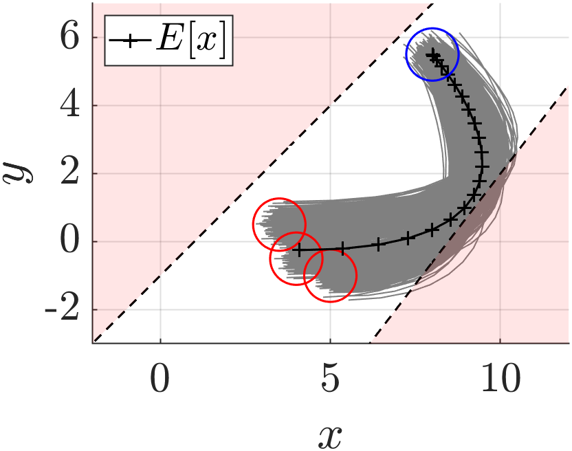
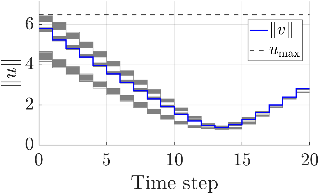
Figure 1: (a) Trajectory and (b) control magnitude when halfplane state constraints are not imposed.

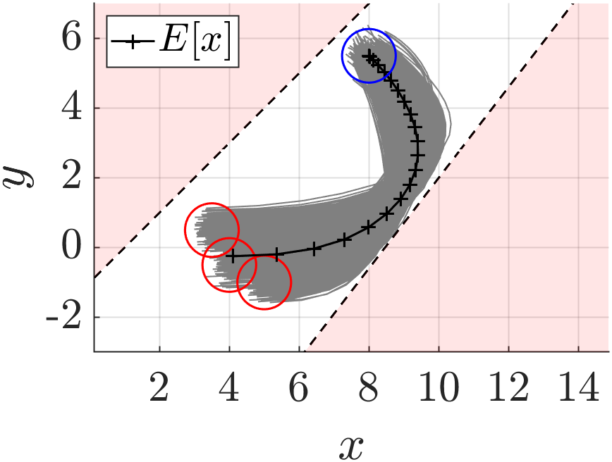
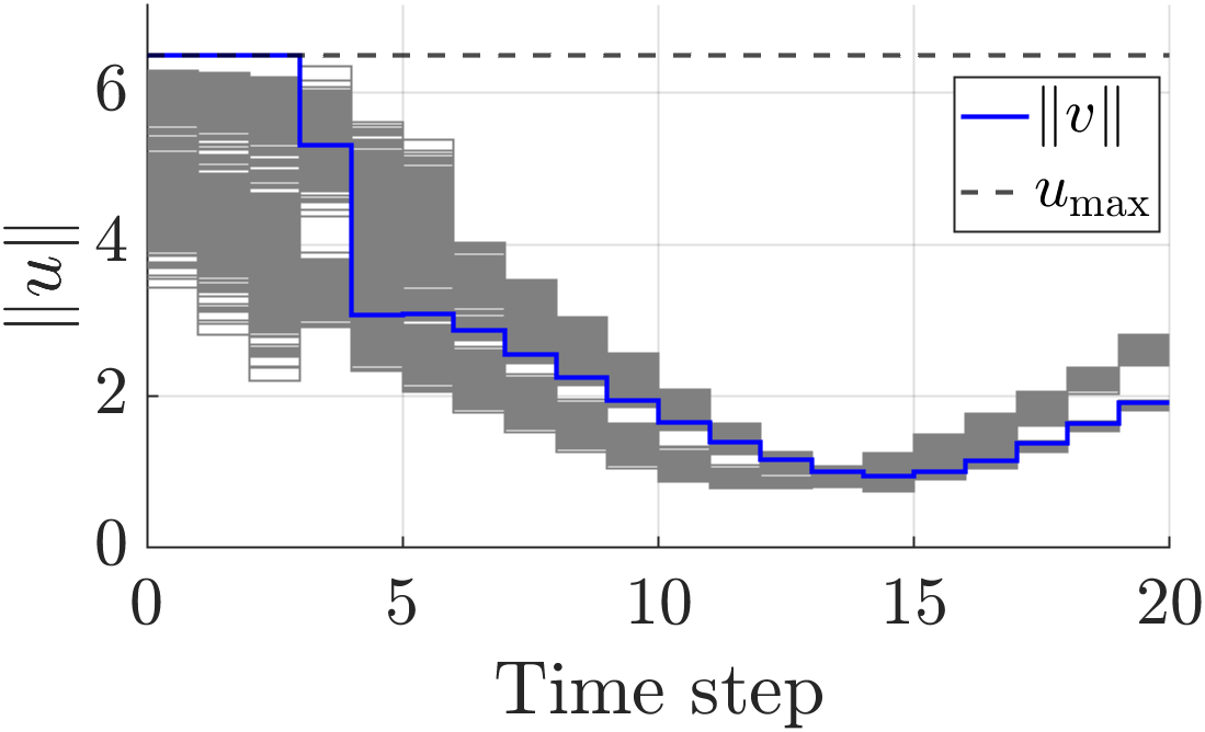
Figure 2: (a) Trajectory and (b) control magnitude when halfplane state constraints are imposed

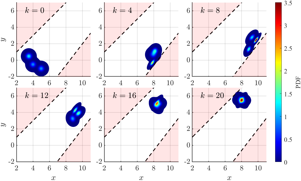
Figure 3: Evolution of density for the path-constrained example. PDF values $<10^{-4}$ are omitted for visualization.

Next, we refine the solution to the state-constrained problem using the proposed IRA algorithm. We choose $\epsilon{=}10^{-2}$ and $\beta{=}0.7$ as the IRA algorithm parameters. The algorithm converges after 13 iterations. The improvement in cost was approximately 5%. We observed that the IRA algorithm is more effective for smaller values of $\Delta,\Gamma$. Fig. 4 compares the Monte Carlo trajectories with and without IRA. Both the mean and outliers of the IRA-refined solution approach the halfplane closer than when it is not employed.

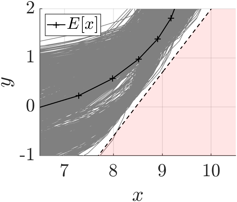
(a) without IRA

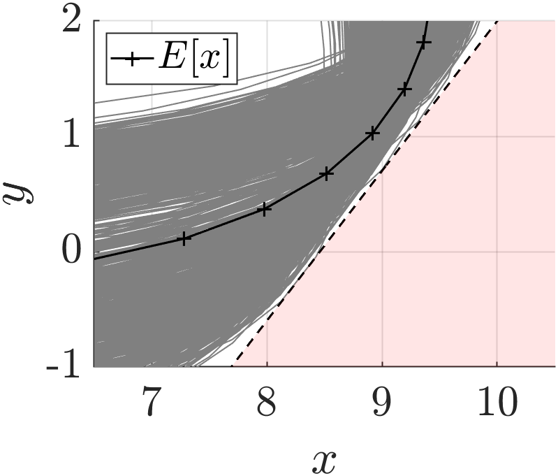
(b) with IRA

Figure 4: Comparison of the trajectory of Monte Carlo samples

The history of cost is shown in Fig. 5. We see that the value decreases monotonically.

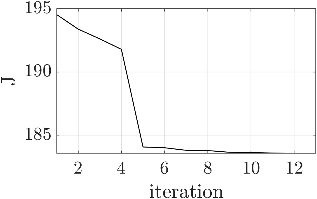
Figure 5: History of cost for the IRA algorithm

Finally, we compare the 2-norm cost for the same settings. The trajectory approaches the target more directly. The terminal covariance constraint is not active. The control magnitude is ‘bang-bang’-like but also shows the multi-modal distribution derived in Proposition 4. The multi-modal structure is especially observable in the switching phase between maximal and minimal inputs.

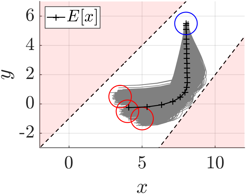
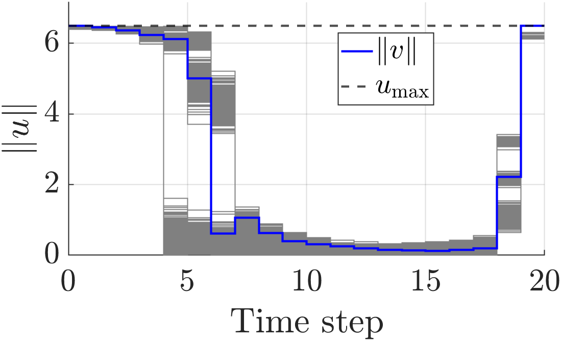
Figure 6: (a) Trajectory and (b) control magnitude for 2-norm cost.

VI Conclusion

We have addressed the problem of Gaussian mixture-to-Gaussian distribution steering under chance constraints. By using a probabilistically chosen affine control policy, the state and control distributions throughout the time horizon are fully characterized by Gaussian mixture models. The original problem is converted to a single semidefinite programming problem, by deriving the deterministic formulations for cost, terminal distributional constraint, and affine/2-norm chance constraints. We also modify the risk allocation algorithm for reduced conservativeness.

References

• [1] A. Hotz and R. E. Skelton, “Covariance control theory,” International Journal of Control, vol. 46, pp. 13–32, July 1987.
• [2] Y. Chen, T. T. Georgiou, and M. Pavon, “Optimal Steering of a Linear Stochastic System to a Final Probability Distribution, Part I,” IEEE Transactions on Automatic Control, vol. 61, pp. 1158–1169, May 2016.
• [3] K. Okamoto, M. Goldshtein, and P. Tsiotras, “Optimal Covariance Control for Stochastic Systems Under Chance Constraints,” IEEE Control Systems Letters, vol. 2, pp. 266–271, Apr. 2018.
• [4] F. Liu, G. Rapakoulias, and P. Tsiotras, “Optimal Covariance Steering for Discrete-Time Linear Stochastic Systems,” Jan. 2023. arXiv:2211.00618 [cs, eess].
• [5] V. Sivaramakrishnan, J. Pilipovsky, M. Oishi, and P. Tsiotras, “Distribution Steering for Discrete-Time Linear Systems with General Disturbances using Characteristic Functions,” in 2022 American Control Conference (ACC), pp. 4183–4190, June 2022.
• [6] K. F. Caluya and A. Halder, “Reflected Schrödinger Bridge: Density Control with Path Constraints,” in 2021 American Control Conference (ACC), (New Orleans, LA, USA), pp. 1137–1142, IEEE, May 2021.
• [7] S. Boone and J. McMahon, “Non-Gaussian Chance-Constrained Trajectory Control Using Gaussian Mixtures and Risk Allocation,” in 2022 IEEE 61st Conference on Decision and Control (CDC), pp. 3592–3597, Dec. 2022.
• [8] M. Ono and B. C. Williams, “Iterative Risk Allocation: A new approach to robust Model Predictive Control with a joint chance constraint,” in 2008 47th IEEE Conference on Decision and Control, pp. 3427–3432, Dec. 2008.
• [9] Z. Hu, W. Sun, and S. Zhu, “Chance constrained programs with Gaussian mixture models,” IISE Transactions, vol. 54, pp. 1117–1130, Dec. 2022.
• [10] Y. Yang, W. Wu, B. Wang, and M. Li, “Analytical Reformulation for Stochastic Unit Commitment Considering Wind Power Uncertainty With Gaussian Mixture Model,” IEEE Transactions on Power Systems, vol. 35, pp. 2769–2782, July 2020.
• [11] K. Ren, H. Ahn, and M. Kamgarpour, “Chance-Constrained Trajectory Planning With Multimodal Environmental Uncertainty,” IEEE Control Systems Letters, vol. 7, pp. 13–18, 2023.
• [12] I. M. Balci and E. Bakolas, “Density Steering of Gaussian Mixture Models for Discrete-Time Linear Systems,” Dec. 2023. arXiv:2311.08500 [cs, eess].
• [13] S. Stergiopoulos, ed., Advanced Signal Processing Handbook: Theory and Implementation for Radar, Sonar, and Medical Imaging Real Time Systems. Boca Raton: CRC Press, July 2017.
• [14] A. P. Dempster, N. M. Laird, and D. B. Rubin, “Maximum Likelihood from Incomplete Data via the EM Algorithm,” Journal of the Royal Statistical Society. Series B (Methodological), vol. 39, no. 1, pp. 1–38, 1977.
• [15] M. Goldshtein and P. Tsiotras, “Finite-horizon covariance control of linear time-varying systems,” in 2017 IEEE 56th Annual Conference on Decision and Control (CDC), pp. 3606–3611, Dec. 2017.
• [16] G. Grimmett and D. Stirzaker, Probability and Random Processes: Fourth Edition. Oxford, New York: Oxford University Press, fourth ed., Sept. 2020.
• [17] S. Chakraborty, “Some Applications of Dirac’s Delta Function in Statistics for More Than One Random Variable,” Applications and Applied Mathematics [electronic only], vol. 3, Jan. 2008.
• [18] E. Bakolas, “Optimal covariance control for discrete-time stochastic linear systems subject to constraints,” in 2016 IEEE 55th Conference on Decision and Control (CDC), (Las Vegas, NV), pp. 1153–1158, IEEE, Dec. 2016.
• [19] L. Blackmore and M. Ono, “Convex Chance Constrained Predictive Control Without Sampling,” in AIAA Guidance, Navigation, and Control Conference, (Chicago, Illinois), American Institute of Aeronautics and Astronautics, Aug. 2009.
• [20] K. Oguri, “Chance-Constrained Control for Safe Spacecraft Autonomy: Convex Programming Approach,” in 2024 American Control Conference (ACC), 2024. (accepted).
• [21] J. Lofberg, “YALMIP : a toolbox for modeling and optimization in MATLAB,” in 2004 IEEE International Conference on Robotics and Automation (IEEE Cat. No.04CH37508), pp. 284–289, Sept. 2004.
• [22] MOSEK ApS, “The MOSEK optimization toolbox for MATLAB manual. Version 10.1.,” 2023.