Unbiased Extremum Seeking Based on Lie Bracket Averaging

Abstract

Extremum seeking is an online, model-free optimization algorithm traditionally known for its practical stability. This paper introduces an extremum seeking algorithm designed for unbiased convergence to the extremum asymptotically, allowing users to define the convergence rate. Unlike conventional extremum seeking approaches utilizing constant gains, our algorithms employ time-varying parameters. These parameters reduce perturbation amplitudes towards zero in an asymptotic manner, while incorporating asymptotically growing controller gains. The stability analysis is based on state transformation, achieved through the multiplication of the input state by asymptotic growth function, and Lie bracket averaging applied to the transformed system. The averaging ensures the practical stability of the transformed system, which, in turn, leads to the asymptotic stability of the original system. Moreover, for strongly convex maps, we achieve exponentially fast convergence. The numerical simulations validate the feasibility of the introduced designs.

I Introduction

Extremum seeking (ES) is a powerful optimization technique that operates in real-time without requiring a detailed model of a scalar-valued convex cost function with multiple inputs. It perturbs the function, estimates the gradient using output feedback and adjusts the input parameters towards their optimal values. However, this method introduces a trade-off. While these perturbations are crucial for ES to learn and adapt, they also prevent the system from reaching the perfect optimum. Instead, they settle into a limit cycle around the optimum. Reducing the size of residual oscillation is crucial as it enables increased power production [10], more precise tuning of design parameters [17], and more accurate localization of leakage sources [8].

Researchers in ES field have developed various methods to eliminate persistent oscillation around the optimum and improve convergence accuracy. An approach in [15] involves a time-varying perturbation amplitude, that decays to zero, by ensuring practical asymptotical convergence to the global extremum despite local extrema. Another approach presented in [16] adjusts the perturbation amplitude based on system output. However, the claim of exponential convergence to optimum in [16] has been shown to be inaccurate theoretically [2] and numerically [6, 7]. Employing Kalman filtering techniques with the feedback of output to dynamically update the amplitude, [11] and [3] achieve asymptotic convergence to a neighborhood of the extremum with diminishing oscillation. Regulating the inputs directly to their unknown optimal values is achieved in [5] and [13] with ES that vanishes at the origin, assuming the optimal value of cost function is known beforehand. Relaxing this restriction, [1], [6], [7], and [14] present control designs that achieve asymptotic convergence of both inputs and outputs to their unknown optimum values. Specifically, [1] achieves this under certain initial conditions, [7] employs time-varying tuning parameters with decaying frequency and amplitude, [6] reduces the size of the search region by estimating the uncertainty set around the optimizer and updating the amplitude accordingly, and [14] adopts an approach with unboundedly growing update rates and frequencies.

In our previous work [19], we introduce a novel ES design called the exponential unbiased extremum seeker (uES). This design achieves a first in the field: exponential and unbiased convergence to the unknown optimum at a user-defined rate. We further expanded on this work in [18] and [20], introducing designs for prescribed-time unbiased convergence and perfect tracking of time-varying optimum, respectively. However, these works rely on the strong convexity of the cost function, limiting the applicability of the developed algorithms. This paper takes a step forward by considering a broader class of cost functions including strongly convex maps, and relaxes the function’s $\mathcal{C}^{4}$ assumption to $\mathcal{C}^{2}$, allowing for continuous differentiability up to the second order. Compared to the existing designs [1], [6], [7], [14], which achieve asymptotic unbiased convergence, our uES design offers a key advantage: convergence at a user-defined asymptotic rate. Additionally, for strongly convex $\mathcal{C}^{2}$ maps, we achieve exponentially fast convergence at a user-defined rate.

Our uES design modifies the alternative ES design [12], which can only ensure practical stability around the optimum, by incorporating time-varying design parameters. In our approach, the update rate and controller gain decay and grow, respectively, at carefully selected asymptotic rates. This enables unbiased convergence to the optimum at the same rate as the decay of the update rate. In cases of strongly convex maps, the asymptotically decaying/growing parameters are replaced by exponential ones to achieve exponential convergence to the optimum.

The structure of this paper is as follows. Section II introduces fundamental stability concepts, which serve as references throughout the paper. Section III outlines the problem formulation. Sections IV and V introduce designs for asymptotic and exponential uES, along with formal stability analysis. Section VI discusses the numerical results. Finally, Section VII concludes the paper.

Notation: We denote the Euclidean norm by $|\cdot|$. The $\delta$-neighborhood of a set $\mathcal{S}\subset\mathbb{R}^{n}$ is denoted by $U_{\delta}^{\mathcal{S}}=\{x\in\mathbb{R}^{n}:\inf_{e\in\mathcal{S}}|x-e|<\delta\}$. The Lie bracket of two vector fields $f,g:\mathbb{R}^{n}\times\mathbb{R}\rightarrow\mathbb{R}^{n}$ with $f(\cdot,t),g(\cdot,t)$ being continuously differentiable is defined by $[f,g](x,t):=\frac{\partial g(x,t)}{\partial x}f(x,t)-\frac{\partial f(x,t)}{\partial x}g(x,t)$. The notation $e_{i}$ corresponds to the $i$th unit vector in $\mathbb{R}^{n}$. $\mathbb{R}^{+}$ denotes the set of non-negative real numbers. We denote the gradient and Hessian of a function $h:\mathbb{R}^{n}\to\mathbb{R}$ by $\nabla h(x)$ and $\nabla^{2}h(x)$, respectively.

II Preliminaries

Consider a control-affine system

$$\dot{x}={}f_{0}(x,t)+\sum_{i=1}^{m}f_{i}(x,t)\sqrt{\omega}u_{i}(\omega t),$$ (1)

where $x\in\mathcal{D}\subseteq\mathbb{R}^{n}$, $x(t_{0})\in\mathcal{D}$, $t_{0}\in\mathbb{R}^{+}$, $\omega>0$, $f_{j}:\mathcal{D}\times\mathbb{R}^{+}\to\mathbb{R}^{n}$ for $j=1,\dots,m$. We compute the Lie bracket system corresponding to (1) as follows

$$\dot{\bar{x}}={}f_{0}(\bar{x},t)+\frac{1}{T}\sum_{{i=1}\atop{j=i+1}}^{m}[f_{i},f_{j}](\bar{x},t)\int_{0}^{T}\int_{0}^{\theta}u_{j}(\theta)u_{i}(\tau)d\tau d\theta,$$ (2)

where $\bar{x}(t_{0})=x(t_{0})$, $T>0$. We recall the following theorem from [4], which defines the concept of practical stability.

Theorem 1

Consider the system (1) and let the following conditions hold:

• $f_{i}\in\mathcal{C}^{2}:\mathcal{D}\times\mathbb{R}^{+}\to\mathbb{R}^{n}$ for $i=0,\dots,q$.

• The functions $|f_{i}(x,t)|$, $\left|\frac{\partial f_{i}(x,t)}{\partial t}\right|$, $\left|\frac{\partial f_{i}(x,t)}{\partial x}\right|$, $\left|\frac{\partial^{2}f_{j}(x,t)}{\partial t\partial x}\right|$, $\left|\frac{\partial[f_{j},f_{k}](x,t)}{\partial t}\right|$, $\left|\frac{\partial[f_{j},f_{k}](x,t)}{\partial x}\right|$ are bounded on each compact set $x\in\mathcal{K}\subset\mathcal{D}$ uniformly in $t\geq t_{0}$, for $i=0,\dots,q$, $j=1,\dots,q$, $k=j,\dots,q$.

• The functions $u_{j}$ are continuous $T$-periodic with some $T>0$, and $\int_{0}^{T}u_{j}(\sigma)d\sigma=0$ for $j=1,\dots,q$.

If a compact set $\mathcal{S}\subset\mathcal{D}$ is locally (globally) uniformly asymptotically stable for (2), then $\mathcal{S}$ is locally (semi-globally) practically uniformly asymptotically stable for (1).

To provide a clear understanding of the concept of practical stability, we present the following definition from [4]:

Definition 1

A compact set $\mathcal{S}\subset\mathbb{R}^{n}$ is said to be locally practically uniformly asymptotically stable for (1) if the following three conditions are satisfied:

• Practical Uniform Stability: For any $\epsilon>0$ there exist $\delta,\omega_{0}>0$ such that for all $t_{0}\in\mathbb{R}^{+}$ and $\omega>\omega_{0}$,

  $$x(t_{0})\in U_{\delta}^{\mathcal{S}}\Rightarrow x(t)\in U_{\epsilon}^{\mathcal{S}},\quad t\in[t_{0},\infty).$$ (3)

• $\delta$-Practical Uniform Attractivity: Let $\delta>0$. For any $\epsilon>0$ there exist $t_{1}\geq 0$ and $\omega_{0}>0$ such that for all $t_{0}\in\mathbb{R}^{+}$ and $\omega>\omega_{0}$,

  $$x(t_{0})\in U_{\delta}^{\mathcal{S}}\Rightarrow x(t)\in U_{\epsilon}^{\mathcal{S}},\quad t\in[t_{0}+t_{1},\infty).$$ (4)

• Practical Uniform Boundedness: For any $\delta>0$ there exist $\epsilon>0$ and $\omega_{0}>0$ such that for all $t_{0}\in\mathbb{R}^{+}$ and $\omega>\omega_{0}$,

  $$x(t_{0})\in U_{\delta}^{\mathcal{S}}\Rightarrow x(t)\in U_{\epsilon}^{\mathcal{S}},\quad t\in[t_{0},\infty).$$ (5)

  Furthermore, if $\delta$-practical uniform attractivity holds for every $\delta>0$, then the compact set $\mathcal{S}$ is said to be semi-globally practically uniformly asymptotically stable for (1).

III Problem Statement

We consider the following optimization problem

$$\min_{\theta\in\mathcal{U}}J(\theta),$$ (6)

where $\theta\in\mathcal{U}\subseteq\mathbb{R}^{n}$ is the input, $J\in\mathcal{C}^{2}:\mathcal{U}\to\mathbb{R}$ is an unknown cost function. We make the following assumptions regarding the unknown static map $J(\cdot)$.

Assumption 1

The cost function $J(\cdot)$ has a unique minimum at $\theta^{*}\in\mathcal{U}$, i.e., $J(\theta^{*})<J(\theta)$ for $\forall\theta\neq\theta^{*}$ with $\nabla J(\theta^{*})=0$.

Assumption 2

There exist constants $a_{1}$, $a_{2}$, $b_{1}$, $b_{2}$, $c_{1}$, $c_{2}>0,\kappa\in\mathbb{N}$ such that

$$a_{1}|\theta-\theta^{*}|^{2\kappa}\leq{} J(\theta)-J(\theta^{*})\leq a_{2}|\theta-\theta^{*}|^{2\kappa},$$ (7)

$$b_{1}|\theta-\theta^{*}|^{2\kappa-1}\leq{} |\nabla J(\theta)|\leq b_{2}|\theta-\theta^{*}|^{2\kappa-1},$$ (8)

$$c_{1}|\theta-\theta^{*}|^{2\kappa-2}\leq{} |\nabla^{2}J(\theta)|\leq c_{2}|\theta-\theta^{*}|^{2\kappa-2}.$$ (9)

Assumption 1 guarantees the existence of a minimum of the function $J(\theta)$ at $\theta=\theta^{*}$. Assumption 2 establishes bounds on the cost function $J(\theta)$, its gradient, and its Hessian, ensuring their growth rates are governed by specific power functions. These bounds play a pivotal role in both algorithm design and stability analysis.

We measure the unknown function $J(\theta)$ in real time as follows

$$y(t)={} J(\theta(t)),\qquad t\in[t_{0},\infty),$$ (10)

in which $y\in\mathbb{R}$ is the output. Our aim is to design ES algorithms using output feedback $y(t)$ in order to achieve the unbiased convergence of $\theta$ to $\theta^{*}$ while simultaneously minimizing the steady state value of $y$, without requiring prior knowledge of either the optimum input $\theta^{*}$ or the function $J(\cdot)$.

In the subsequent sections, we present two types of unbiased ES algorithms, namely asymptotic uES, and exponential uES, which respectively achieve the aforementioned objective asymptotically, and exponentially. To provide a visual representation, the uES designs introduced are depicted schematically in Fig. 1. Additionally, relevant information such as amplitude, and gain functions can be found in Table I. For $\kappa\geq 1$, the asymptotic uES method gradually diminishes the amplitudes (i.e., update rates) towards zero in an asymptotic manner, while employing asymptotically growing controller gains. On the other hand, for $\kappa=1$, exponential uES employs exponentially decaying update rates as well as exponentially growing controller gains, to achieve the exponential and unbiased convergence to the optimum.

Remark 1

In the unbiased ES designs depicted in Fig. 1, the gain $k_{i}\varphi(t)$ experiences either asymptotic or exponential growth based on the chosen ES type, while the update rate $\nu(t)\sqrt{\alpha_{i}\omega_{i}}$ experiences asymptotic or exponential decay corresponding to the specific ES type. The crucial aspect of our designs is that the high-pass filtered state $y-\eta$ decays to zero at least as fast as the gain $k_{i}\varphi(t)$ grows, ensuring the boundedness of the resulting signal. For a more detailed analysis, refer to Theorem 2 and 3.

IV Asymptotic uES for $\kappa\geq 1$

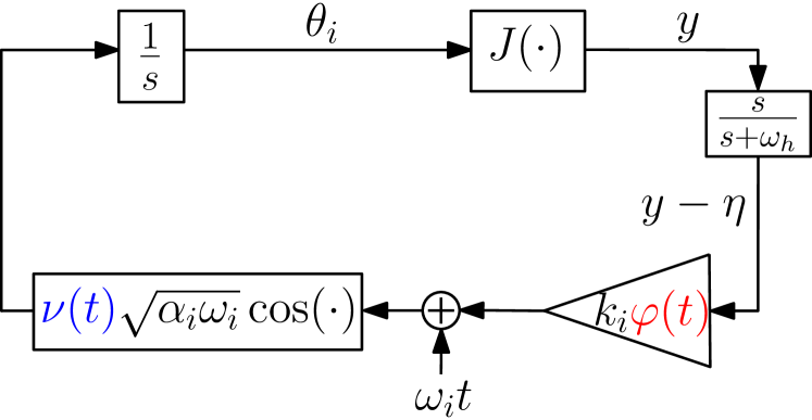
Figure 1: Unbiased ES scheme for the $i$th element $\theta_{i}$ of $\theta$. Refer to Table I for the functions $\nu(t),\varphi(t)$.

	$\nu(t)$	$\varphi(t)$
Asymptotic uES	$(1+\beta\ (t-t_{0}))^{-\frac{1}{v}}$	$(1+\beta\ (t-t_{0}))^{\frac{r}{v}}$
for $\kappa\geq 1$
Exponential uES	$e^{-\lambda(t-t_{0})}$	$e^{2\lambda(t-t_{0})}$
for $\kappa=1$

TABLE I: Time-varying functions used in asymptotic and exponential uES schemes where $\beta,\lambda>0,v>2\kappa-r\geq 0$.

The convergence result is stated in the following theorem.

Theorem 2

Consider the following asymptotic uES design

$$\begin{cases}\begin{aligned} \dot{\theta}={}&\frac{1}{\xi(t)}\sum_{i=1}^{n}\sqrt{\alpha_{i}\omega_{i}}e_{i}\cos\Big{(}\omega_{i}t+k_{i}\xi^{r}(t)(J(\theta)-\eta)\Big{)},\\ \dot{\eta}={}&-\omega_{h}\eta+\omega_{h}J(\theta),\end{aligned}\end{cases}$$ (11)

with the asymptotically growing function

$$\xi(t)={}(1+\beta(t-t_{0}))^{\frac{1}{v}},\qquad t\in[t_{0},\infty).$$ (12)

Let $\omega_{i}=\omega\hat{\omega}_{i}$ such that $\hat{\omega}_{i}\neq\hat{\omega}_{j}$ $\forall i\neq j$, $t_{0}\geq 0$, $\alpha_{i},k_{i},\beta,\omega_{h}>0$ $\forall i=1,\dots,n$ and $v>2\kappa-r\geq 0$. Let Assumptions 1 and 2 hold. Then, there exists $\omega^{*}>0$ such that for all $\omega>\omega^{*}$, the followings hold

• $\theta(t)\to\theta^{*}$ asymptotically at the rate of $1/\xi(t)$,

• $\eta(t),y(t)\to J(\theta^{*})$ asymptotically at the rate of $1/\xi^{2\kappa}(t)$.

Proof:

Let us proceed through the proof step by step.

Step 1: State transformation. Let us consider the following transformations

$$\theta_{f}={} \xi(t)(\theta-\theta^{*}),$$ (13)

$$\eta_{f}={} \xi^{2\kappa}(t)(\eta-J(\theta^{*})),$$ (14)

which transform (11) to

$$\begin{cases}\begin{aligned} \dot{\theta}_{f}={}&\frac{\beta}{v\xi^{v}(t)}{\theta}_{f}+\sum_{i=1}^{n}\sqrt{\alpha_{i}\omega_{i}}e_{i}\cos\bigg{(}\omega_{i}t+k_{i}\xi^{r}(t)\\ &\times\left(J_{f}(\theta_{f},\xi(t))-\frac{1}{\xi^{2\kappa}(t)}{\eta}_{f}\right)\bigg{)},\qquad\quad\\ \dot{\eta}_{f}={}&\left(\frac{2\beta\kappa}{v\xi^{v}(t)}-\omega_{h}\right)\eta_{f}+\omega_{h}\xi^{2\kappa}(t)J_{f}(\theta_{f},\xi(t)),\end{aligned}\end{cases}$$ (15)

with

$$J_{f}(\theta_{f},\xi(t))={} J(\theta_{f}/\xi(t)+\theta^{*})-J(\theta^{*}).$$ (16)

The initial and most critical step in our analysis relies on transformations (13), (14). These establish a precondition: once we demonstrate the stability of the transformed system (15), the asymptotic convergence of $\theta$ to $\theta^{*}$ and $\eta$ to $J(\theta^{*})$ naturally follows. To analyze the stability of (15), we employ the Lie bracket averaging technique. As a first step, we rewrite the $\theta_{f}$-system in (15) by expanding the cosine term, as shown below

$$\dot{\theta}_{f}={} \frac{\beta}{v\xi^{v}(t)}{\theta}_{f}+\sum_{i=1}^{n}\sqrt{\alpha_{i}\omega_{i}}e_{i}\cos(\omega_{i}t)$$

$$\times\cos\left(k_{i}\xi^{r}(t)\left(J_{f}(\theta_{f},\xi(t))-\frac{1}{\xi^{2\kappa}(t)}{\eta}_{f}\right)\right)$$

$$-\sum_{i=1}^{n}\sqrt{\alpha_{i}\omega_{i}}e_{i}\sin(\omega_{i}t)$$

$$\times\sin\left(k_{i}\xi^{r}(t)\left(J_{f}(\theta_{f},\xi(t))-\frac{1}{\xi^{2\kappa}(t)}{\eta}_{f}\right)\right).$$ (17)

Next, we integrate the $\eta_{f}$-system from (15) with the transformed $\theta_{f}$-system (17) to construct the following system

$$\begin{bmatrix}\dot{\theta}_{f}\\ \dot{\eta}_{f}\end{bmatrix}={} b_{0}(\theta_{f},\eta_{f},t)+\sum_{i=1}^{n}b_{c,i}(\theta_{f},\eta_{f},t)\sqrt{\omega_{i}}\cos(\omega_{i}t)$$

$$-b_{s,i}(\theta_{f},\eta_{f},t)\sqrt{\omega_{i}}\sin(\omega_{i}t),$$ (18)

where

$$b_{0}(\theta_{f},\eta_{f},t)$$

$$=\begin{bmatrix}\frac{\beta}{v\xi^{v}(t)}\theta_{f}\\ \left(\frac{2\beta\kappa}{v\xi^{v}(t)}-\omega_{h}\right)\eta_{f}+\omega_{h}\xi^{2\kappa}(t)J_{f}(\theta_{f},\xi(t))\end{bmatrix},$$ (19)

$$b_{c,i}(\theta_{f},\eta_{f},t)$$

$$=\begin{bmatrix}\sqrt{\alpha_{i}}e_{i}\cos\Big{(}k_{i}\xi^{r}(t)\left(J_{f}(\theta_{f},\xi(t))-\frac{{\eta}_{f}}{\xi^{2\kappa}(t)}\right)\Big{)}\\ 0\end{bmatrix},$$ (20)

$$b_{s,i}(\theta_{f},\eta_{f},t)$$

$$=\begin{bmatrix}\sqrt{\alpha_{i}}e_{i}\sin\Big{(}k_{i}\xi^{r}(t)\left(J_{f}(\theta_{f},\xi(t))-\frac{{\eta}_{f}}{\xi^{2\kappa}(t)}\right)\Big{)}\\ 0\end{bmatrix}.$$ (21)

Step 2: Feasibility analysis of (18) for averaging. To ensure the applicability of Lie bracket averaging, we need to verify that (18) satisfies the boundedness assumption outlined in Theorem 1. Towards this end, let $\mathcal{M}\subset\mathcal{U}$ and $\mathcal{Z}\subset\mathbb{R}$ be compact sets, and consider the bound (7) in Assumption 1. This leads to the following bound

$$\xi^{2\kappa}(t)J_{f}(\theta_{f},\xi(t))\leq{} a_{1}|\theta_{f}|^{2\kappa}.$$ (22)

Based on the bound (22), we establish the boundedness of $|b_{0}(\theta_{f},\eta_{f},t)|$, $|b_{c,i}(\theta_{f},\eta_{f},t)|$, and $|b_{s,i}(\theta_{f},\eta_{f},t)|$ for $(t,\theta_{f},\eta_{f})\in[t_{0},\infty)\times\mathcal{M}\times\mathcal{Z}$. Noting from (13) that

$$\frac{d\theta}{d\theta_{f}}={}\frac{1}{\xi(t)},$$ (23)

and recalling the bounds in Assumption 2, we derive the following inequalities

$$\xi^{2\kappa}(t)\left|\frac{\partial J_{f}(\theta_{f},\xi(t))}{\partial\theta_{f}}\right|={} \xi^{2\kappa-1}(t)\left|\frac{\partial J(\theta)}{\partial\theta}\right|\leq{}b_{2}\theta_{f}^{2\kappa-1},$$ (24)

$$\xi^{2\kappa}(t)\left|\frac{\partial J_{f}(\theta_{f},\xi(t))}{\partial t}\right|={} \xi^{2\kappa}(t)\left|\frac{\partial J(\theta)}{\partial\theta}\left(-\frac{\theta_{f}\dot{\xi}(t)}{\xi^{2}(t)}\right)\right|,$$

$$\leq{} \frac{\beta b_{2}}{v\xi^{v}(t)}|\theta_{f}|^{2\kappa},$$ (25)

$$\xi^{2\kappa}(t)\left|\frac{\partial^{2}J_{f}(\theta_{f},\xi(t))}{\partial\theta_{f}\partial t}\right|={} \xi^{2\kappa}(t)\left|\frac{\partial}{\partial t}\left(\frac{\partial J(\theta)}{\partial\theta}\frac{1}{\xi(t)}\right)\right|,$$

$$\leq{}\xi^{2\kappa-2}(t)\left(\left|\frac{\partial J(\theta)}{\partial\theta}\right|\dot{\xi}(t)+\left|\frac{\partial^{2}J(\theta)}{\partial\theta^{2}}\right|\right),$$

$$\leq{}\frac{\beta b_{2}}{v\xi^{v}(t)}|\theta_{f}|^{2\kappa-1}+c_{2}|\theta_{f}|^{2\kappa-2},$$ (26)

$$\xi^{2\kappa}(t)\left|\frac{\partial^{2}J_{f}(\theta_{f},\xi(t))}{\partial\theta_{f}^{2}}\right|={} \xi^{2\kappa-2}(t)\left|\frac{\partial^{2}J(\theta)}{\partial\theta^{2}}\right|\leq{}c_{2}\theta_{f}^{2\kappa-2},$$ (27)

which are bounded for $(t,\theta_{f},\eta_{f})\in[t_{0},\infty)\times\mathcal{M}\times\mathcal{Z}$. Considering the bounds (22), (24)–(27), we establish the boundedness of $\left|\frac{\partial b_{0}(\theta_{f},\eta_{f},t)}{\partial\theta_{f}}\right|$, $\left|\frac{\partial b_{0}(\theta_{f},\eta_{f},t)}{\partial\eta_{f}}\right|$, $\left|\frac{\partial b_{0}(\theta_{f},\eta_{f},t)}{\partial t}\right|$, $\left|\frac{\partial b_{c,i}(\theta_{f},\eta_{f},t)}{\partial\theta_{f}}\right|$, $\left|\frac{\partial b_{s,i}(\theta_{f},\eta_{f},t)}{\partial\theta_{f}}\right|$, $\left|\frac{\partial b_{c,i}(\theta_{f},\eta_{f},t)}{\partial\eta_{f}}\right|$, $\left|\frac{\partial b_{s,i}(\theta_{f},\eta_{f},t)}{\partial\eta_{f}}\right|$, $\left|\frac{\partial b_{c,i}(\theta_{f},\eta_{f},t)}{\partial t}\right|$, $\left|\frac{\partial b_{s,i}(\theta_{f},\eta_{f},t)}{\partial t}\right|$, $\left|\frac{\partial^{2}b_{s,i}(\theta_{f},\eta_{f},t)}{\partial\theta_{f}\partial t}\right|$, $\left|\frac{\partial^{2}b_{c,i}(\theta_{f},\eta_{f},t)}{\partial\theta_{f}\partial t}\right|$, $\left|\frac{\partial^{2}b_{s,i}(\theta_{f},\eta_{f},t)}{\partial\eta_{f}\partial t}\right|$, and $\left|\frac{\partial^{2}b_{c,i}(\theta_{f},\eta_{f},t)}{\partial\eta_{f}\partial t}\right|$ for $r\leq 2\kappa$ within the domain $(t,\theta_{f},\eta_{f})\in[t_{0},\infty)\times\mathcal{M}\times\mathcal{Z}$. Next, we compute the following Lie bracket

$$\begin{bmatrix}b_{c,i}(\theta_{f},\eta_{f},t)&b_{s,i}(\theta_{f},\eta_{f},t)\end{bmatrix}$$

$$={} k_{i}\sqrt{\alpha_{i}}\xi^{r}(t)\begin{bmatrix}e_{i}\frac{\partial J_{f}(\theta_{f},\xi(t))}{\partial{\theta}_{f}}\cos(\rho)&-e_{i}\frac{1}{\xi^{2\kappa}(t)}\cos(\rho)\\ 0&0\end{bmatrix}$$

$$\times b_{c,i}(\theta_{f},\eta_{f},t)$$

$$+k_{i}\sqrt{\alpha_{i}}\xi^{r}(t)\begin{bmatrix}e_{i}\frac{\partial J_{f}(\theta_{f},\xi(t))}{\partial{\theta}_{f}}\sin(\rho)&-e_{i}\frac{1}{\xi^{2\kappa}(t)}\sin(\rho)\\ 0&0\end{bmatrix}$$

$$\times b_{s,i}(\theta_{f},\eta_{f},t),$$

$$={} k_{i}\alpha_{i}\xi^{r}(t)\begin{bmatrix}e_{i}\frac{\partial J_{f}(\theta_{f},\xi(t))}{\partial{\theta}_{f,i}}\\ 0\end{bmatrix},$$ (28)

where

$$\rho={}k_{i}\xi^{r}(t)\left(J_{f}(\theta_{f},\xi(t))-{\eta}_{f}/\xi^{2\kappa}(t)\right).$$ (29)

The boundedness of $\left|\frac{\partial[b_{c,i}(\theta_{f},\eta_{f},t),\,b_{s,i}(\theta_{f},\eta_{f},t)]}{\partial\theta_{f}}\right|$ and $\left|\frac{\partial[b_{c,i}(\theta_{f},\eta_{f},t),\,b_{s,i}(\theta,\eta_{f},t)]}{\partial t}\right|$ for $r\leq 2\kappa$ within the domain $(t,\theta_{f},\eta_{f})\in[t_{0},\infty)\times\mathcal{M}\times\mathcal{Z}$ is established by revisiting the bounds (24)–(27). Additionally, it should be noted that $\left|\frac{\partial[b_{c,i}(\theta_{f},\eta_{f},t),\,b_{s,i}(\theta_{f},\eta_{f},t)]}{\partial\eta_{f}}\right|=0$. As a result, we fulfill the boundedness requirement for Lie bracket averaging.

Step 3: Lie bracket averaging. We derive the Lie bracket system for (18) as follows

$$\begin{bmatrix}\dot{\bar{\theta}}_{f}\\ \dot{\bar{\eta}}_{f}\end{bmatrix}={} b_{0}(\bar{\theta}_{f},\bar{\eta}_{f},t)-\frac{1}{2}\sum_{i=1}^{n}\begin{bmatrix}b_{c,i}(\bar{\theta}_{f},\bar{\eta}_{f},t)&b_{s,i}(\bar{\theta}_{f},\bar{\eta}_{f},t)\end{bmatrix}.$$ (30)

Considering (19) and (28), we can express (30) as

$$\begin{cases}\begin{aligned} \dot{\bar{\theta}}_{f}={}&\frac{\beta}{v\xi^{v}(t)}\bar{\theta}_{f}-\sum_{i=1}^{n}\frac{k_{i}\alpha_{i}}{2}\xi^{r}(t)e_{i}\frac{\partial J_{f}(\bar{\theta}_{f},\xi(t))}{\partial\bar{\theta}_{f,i}},\qquad\quad\\ \dot{\bar{\eta}}_{f}={}&\left(\frac{2\beta\kappa}{v\xi^{v}(t)}-\omega_{h}\right)\bar{\eta}_{f}+\omega_{h}\xi^{2\kappa}(t)J_{f}(\bar{\theta}_{f},\xi(t)).\end{aligned}\end{cases}$$ (31)

Step 4: Stability of average system. Let us consider the following Lyapunov function

$$V(\bar{\theta}_{f},\xi(t))=\xi^{2\kappa}(t)J_{f}(\bar{\theta}_{f},\xi(t)).$$ (32)

In light of Assumption 2, we can establish lower and upper bounds for the Lyapunov function as

$$a_{1}|\bar{\theta}_{f}|^{2\kappa}\leq V(\bar{\theta}_{f},\xi(t))\leq a_{2}|\bar{\theta}_{f}|^{2\kappa}.$$ (33)

Considering Assumption 2 and using (31), (33), we compute the time derivative of (32) as

$$\dot{V}\leq -2\beta\kappa\xi^{2\kappa-v}(t)J_{f}(\bar{\theta}_{f},\xi(t))-\xi^{2\kappa}(t)\frac{\partial J_{f}(\bar{\theta}_{f},\xi(t))}{\partial\bar{\theta}_{f}}\dot{\bar{\theta}}_{f},$$

$$\leq -\frac{b_{1}^{2}}{2}(k\alpha)_{\text{min}}\xi^{-2\kappa+r}|\bar{\theta}_{f}|^{4\kappa-2}+\frac{\left(2\kappa a_{2}+b_{2}\right)\beta}{v\xi^{v}(t)}|\bar{\theta}_{f}|^{2\kappa},$$

$$\leq -\frac{b_{1}^{2}}{2a_{2}}(k\alpha)_{\text{min}}\xi^{-2\kappa+r}V^{\frac{2\kappa-1}{\kappa}}+\frac{\left(2\kappa a_{2}+b_{2}\right)\beta}{a_{1}v\xi^{v}(t)}V,$$ (34)

where $(k\alpha)_{\text{min}}=\min\{k_{i}\alpha_{i}\}$ for $i=1,\dots,n$. By substituting (12) into (34), we get

$$\dot{V}\leq{} -\frac{(k\alpha)_{\text{min}}b_{1}^{2}}{2a_{2}\left(1+\beta(t-t_{0})\right)^{\frac{2\kappa-r}{v}}}V^{\frac{2\kappa-1}{\kappa}}$$

$$+\frac{\left(2\kappa a_{2}+b_{2}\right)\beta}{a_{1}v\left(1+\beta(t-t_{0})\right)}V.$$ (35)

For the stability analysis of (35), we consider two different cases for $\kappa$:

Case 1: $\kappa=1$. Applying the comparison principle to (35), we derive

$$V(t)\leq{} e^{-\frac{(k\alpha)_{\text{min}}b_{1}^{2}}{2a_{2}}(t-t_{0})}(1+\beta(t-t_{0}))^{\frac{\left(2\kappa a_{2}+b_{2}\right)}{a_{1}v}}V(t_{0})$$ (36)

for $r=2$, and

$$V(t)\leq{} e^{-\frac{(k\alpha)_{\text{min}}b_{1}^{2}}{2a_{2}\beta(1-(2\kappa-r)/v)}(1+\beta(t-t_{0}))^{1-(2\kappa-r)/v}}$$

$$\times(1+\beta(t-t_{0}))^{\frac{\left(2\kappa a_{2}+b_{2}\right)}{a_{1}v}}V(t_{0})$$ (37)

for $r<2$. Further employing L’Hôpital’s rule, we establish the uniform asymptotic stability of the averaged $\bar{\theta}_{f}$-system for all $k_{i},\alpha_{i}>0,i=1,\dots,n$.

Case 2: $\kappa>1$. Note that (35) takes the form of (54). Applying Lemma 1, we deduce the uniform asymptotic stability of the averaged $\bar{\theta}_{f}$-system for all $k_{i},\alpha_{i}>0,i=1,\dots,n$.

In addition to establishing the asymptotic stability of the $\bar{\theta}_{f}$-system, we also need to confirm the asymptotic stability of the $\bar{\eta}_{f}$-system in (31). We first examine the unforced system $\dot{\bar{\eta}}_{f}={}\left(\frac{2\beta\kappa}{v\xi^{v}(t)}-\omega_{h}\right)\bar{\eta}_{f}$, which yields the following solution

$$\bar{\eta}_{f}(t)=\xi^{\frac{2\kappa}{v}}(t)e^{-\omega_{h}(t-t_{0})}\bar{\eta}_{f}(t_{0}).$$ (38)

Therefore, the unforced system is exponentially stable at the origin. Furthermore, by revisiting the bound (22), the input of the $\bar{\eta}_{f}$-system, $\omega_{h}J_{f}(\bar{\theta}_{f},\xi(t))\xi^{2\kappa}(t)$, is upper bounded by $\omega_{h}a_{1}|\theta_{f}|^{2\kappa}$. Consequently, the $\bar{\eta}_{f}$-system is input-to-state stable according to [9, Lemma 4.6] and uniformly asymptotically stable at the origin.

Step 5: Lie bracket averaging theorem. Given the uniform asymptotic stability established for the averaged system in (31) in Step 4, we conclude from Theorem 1 that the origin of the transformed system (15) is practically uniformly asymptotically stable.

Step 6: Convergence to extremum. Considering the result in Step 5 and recalling from (12), (13) that

$$\theta=\theta^{*}+\frac{1}{(1+\beta(t-t_{0}))^{\frac{1}{v}}}\theta_{f},$$ (39)

we conclude the asymptotic convergence of $\theta(t)$ to $\theta^{*}$ at the rate of $1/\xi(t)$. This implies the asymptotic convergence of the output $y(t)$ and the filtered state $\eta(t)$ to $J(\theta^{*})$ at the rate of $1/\xi^{2\kappa}(t)$, based on (7), (13), (14), and thereby concludes the proof of Theorem 2. ∎

V Exponential uES for $\kappa=1$

The convergence result is stated in the following theorem.

Theorem 3

Consider the following exponential uES design

$$\begin{cases}\begin{aligned} \dot{\theta}={}&\frac{1}{\zeta(t)}\sum_{i=1}^{n}\sqrt{\alpha_{i}\omega}_{i}e_{i}\cos\left(\omega_{i}t+k_{i}\zeta^{2}(t)(J(\theta)-\eta)\right),\\ \dot{\eta}={}&-\omega_{h}\eta+\omega_{h}J(\theta),\end{aligned}\end{cases}$$ (40)

with the exponentially growing function

$$\zeta(t)={}e^{\lambda(t-t_{0})},\quad\lambda>0,\quad t\in[t_{0},\infty).$$ (41)

Let $\omega_{i}=\omega\hat{\omega}_{i}$ such that $\hat{\omega}_{i}\neq\hat{\omega}_{j}$ $\forall i\neq j$, $t_{0}\geq 0$, and

$$k_{i}\alpha_{i}>{} 2\lambda a_{2}(2a_{2}+b_{2})/(a_{1}b_{1}^{2}),$$ (42)

$$\omega_{h}>{} 2\lambda$$ (43)

for all $i=1,\dots,n$. Let Assumptions 1 and 2 hold. Then, for $\kappa=1$, there exists $\omega^{*}>0$ such that for all $\omega>\omega^{*}$, the followings hold

• $\theta(t)\to\theta^{*}$ exponentially at the rate of $\lambda$,

• $\eta(t),y(t)\to J(\theta^{*})$ exponentially at the rate of $2\lambda$.

Proof:

Let us proceed through the proof step by step.

Step 1: State transformation. Let us consider the following transformations

$$\theta_{f}={} \zeta(t)(\theta-\theta^{*}),$$ (44)

$$\eta_{f}={} \zeta^{2}(t)(\eta-J(\theta^{*})).$$ (45)

Using (44) and (45), we transform (40) to

$$\begin{cases}\begin{aligned} \dot{\theta}_{f}={}&\lambda{\theta}_{f}+\sum_{i=1}^{n}\sqrt{\alpha_{i}\omega_{i}}e_{i}\cos\bigg{(}\omega_{i}t+k_{i}\zeta^{2}(t)\\ &\times\left(J_{f}(\theta_{f},\zeta(t))-\frac{1}{\zeta^{2}(t)}{\eta}_{f}\right)\bigg{)},\\ \dot{\eta}_{f}={}&(2\lambda-\omega_{h})\eta_{f}+\omega_{h}\zeta^{2}(t)J_{f}(\theta_{f},\zeta(t)),\end{aligned}\end{cases}$$ (46)

with

$$J_{f}(\theta_{f},\zeta(t))={} J(\theta_{f}/\zeta(t)+\theta^{*})-J(\theta^{*}).$$ (47)

Step 2: Lie bracket averaging and stability analysis. The feasibility of the error system (46) for Lie bracket averaging can be verified analogously to Step 2 in the proof of Theorem 2. In contrast to (31), the average of (46) results in

$$\begin{cases}\begin{aligned} \dot{\bar{\theta}}_{f}={}&\lambda{\bar{\theta}}_{f}-\sum_{i=1}^{n}\frac{k_{i}\alpha_{i}}{2}e_{i}\zeta^{2}(t)\frac{\partial J_{f}(\bar{\theta}_{f},\zeta(t))}{\partial\bar{\theta}_{f,i}},\\ \dot{\bar{\eta}}_{f}={}&(2\lambda-\omega_{h})\bar{\eta}_{f}+\omega_{h}\zeta^{2}(t)J_{f}(\bar{\theta}_{f},\zeta(t)).\end{aligned}\end{cases}$$ (48)

Consider the following Lyapunov function

$$V=\zeta^{2}(t)J_{f}(\bar{\theta}_{f},\zeta(t)).$$ (49)

We leverage Assumption 2 to derive the following bounds for the Lyapunov function

$$a_{1}|\bar{\theta}_{f}|^{2}\leq V(\bar{\theta}_{f},\zeta(t))\leq a_{2}|\bar{\theta}_{f}|^{2}.$$ (50)

Taking Assumption 2 into consideration and using (48), (50), we compute the time derivative of (49) as

$$\dot{V}\leq{} 2\lambda\zeta^{2}(t)J_{f}(\bar{\theta}_{f},\zeta(t))-\zeta^{2}(t)\frac{\partial J_{f}(\bar{\theta}_{f},\zeta(t))}{\partial\bar{\theta}_{f}}\dot{\bar{\theta}}_{f},$$

$$\leq{} \lambda(2a_{2}+b_{2})|\bar{\theta}_{f}|^{2}-\frac{(k\alpha)_{\text{min}}}{2}b_{1}^{2}|\bar{\theta}_{f}|^{2},$$

$$\leq{} \left(\frac{\lambda(2a_{2}+b_{2})}{a_{1}}-\frac{(k\alpha)_{\text{min}}}{2a_{2}}b_{1}^{2}\right)V,$$ (51)

from which we conclude the uniform asymptotic stability of the averaged $\bar{\theta}_{f}$-system for $k_{i}\alpha_{i}$ satisfying (42). To establish the asymptotic stability of the $\bar{\eta}_{f}$-system, we analyze its unforced dynamics, governed by $\dot{\bar{\eta}}_{f}=(2\lambda-\omega_{h})\bar{\eta}_{f}$. This system is exponentially stable at the origin for $\omega_{h}>2\lambda$. The input-to-state stability of the $\bar{\eta}_{f}$-system is established by noting from (7) that $|\omega_{h}\zeta^{2}(t)J_{f}(\bar{\theta}_{f},\zeta(t))|\leq\omega_{h}a_{2}|\bar{\theta}_{f}|^{2}$. Hence, the asymptotic convergence of $\bar{\theta}_{f}$ results in the asymptotic convergence of $\bar{\eta}_{f}$ as well.

Step 3: Lie bracket averaging theorem. Given the uniform asymptotic stability established for the averaged system in (48) in Step 2, we conclude from Theorem 1 that the origin of the transformed system (46) is practically uniformly asymptotically stable.

Step 4: Convergence to extremum. Considering the result in Step 3 and recalling from (41), (44) that

$$\theta=\theta^{*}+e^{-\lambda(t-t_{0})}\theta_{f},$$ (52)

we conclude the exponential convergence of $\theta(t)$ to $\theta^{*}$ at the rate of $\lambda$. This implies the exponential convergence of the output $y(t)$ and the filtered state $\eta(t)$ to $J(\theta^{*})$ at the rate of $2\lambda$, as evident from (7), (44), (45), and completes the proof of Theorem 3. ∎

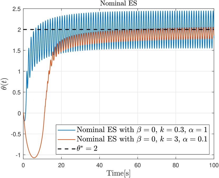
Figure 2: The trajectories of the nominal ES [12] with two distinct parameter sets.

VI Numerical Simulation

In this section, we conduct a numerical simulation to assess the performance of the developed asymptotic uES design. Our objective is to demonstrate its capability to achieve unbiased convergence to the optimum at a user-defined asymptotic rate. We consider the optimization problem (6) with the following nonlinear map

$$J(\theta)={}1+(\theta-2)^{4}.$$ (53)

Note that the function (53) has a unique minimum at $\theta^{*}=2$ and satisfies Assumption 2 with $\kappa=2$. To provide a basis for comparison, we use the nominal ES introduced in [12]. Setting $\beta=0$ in the asymptotic uES (11), our design simplifies to the nominal approach. In all simulations, initial conditions are set to zero, and the oscillation frequency and high-pass filter frequency are set to $\omega=5$ and $\omega_{h}=3$, respectively.

In Figure 2, we depict the trajectories of the nominal ES with two distinct parameter sets. We observe that the nominal ES with $k=0.3$ and $\alpha=1$ converges to a large neighborhood of the optimum due to the high $\alpha$. To reduce the size of the steady-state oscillation, one might consider decreasing $\alpha$ from $1$ to $0.1$, while simultaneously increasing the gain $k$ from $0.3$ to $3$ to maintain the same convergence rate. However, as observed in Figure 2, such adjustment leads to poorer transient performance, with an initial deviation in the opposite direction, despite the reduced oscillations at the steady state compared to one with higher amplitude. Our design, illustrated in Figure 3, addresses this issue. We employ the asymptotic uES (11) with $v=1/3$, $r=4$, $\beta=0.1$, $k=0.3$, $\alpha=1$. It starts with a high $\alpha=1$ and low $k=0.3$, and as $\xi(t)$ increases over time, the input settles to its optimum value with good transient performance. The chosen parameters ensure a convergence rate of $1/(1+0.1t)^{3}$.

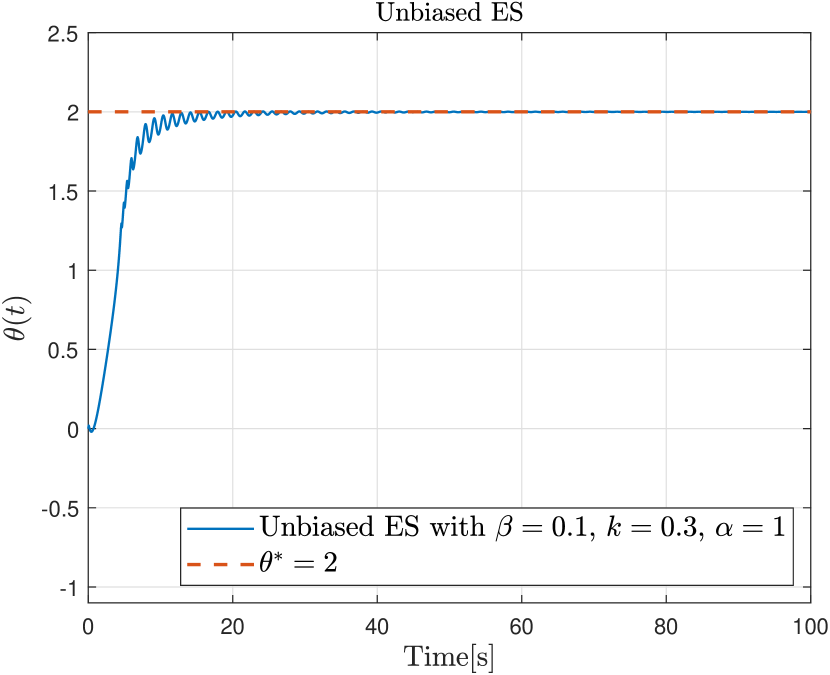
Figure 3: The trajectory of the asymptotic uES (11) with a convergence rate of $1/(1+0.1t)^{3}$.

VII Conclusion

We introduce an ES algorithm that achieves asymptotic unbiased convergence to the unknown optimum. A unique feature of the developed design is that users can pre-define the convergence rate based on the convexity of the cost function. The result is achieved using time-varying parameters, which gradually diminish perturbation amplitudes to zero while increasing controller gains at an asymptotic rate. This strategy can be interpreted within the exploration vs. exploitation paradigm as gradually shifting from exploration to exploitation. Additionally, for strongly convex maps, we present an uES with exponentially fast convergence as an alternative to the classical averaging-based exponential uES introduced in [19].

Appendix A Additional Lemma

Lemma 1

The system

$$\dot{\mathcal{V}}={} -\frac{\varepsilon_{1}}{(1+\beta(t-t_{0}))^{p}}\mathcal{V}^{q}+\frac{\varepsilon_{2}}{(1+\beta(t-t_{0}))}\mathcal{V}$$ (54)

for $t\geq t_{0}$, where $\mathcal{V}\in\mathbb{R}$, $t_{0}\geq 0$, $p<1,q>1$ and $\mathcal{V}(t_{0})$, $\beta$, $\varepsilon_{1}$, $\varepsilon_{2}>0$, is uniformly asymptotically stable.

Proof:

Subtracting $\frac{\varepsilon_{2}}{(1+\beta(t-t_{0}))}\mathcal{V}$ from both sides of (54) and multiplying the resulted expression on the left and right by $(1-q)\mathcal{V}^{-q}$, we get

$$(1-q)\dot{\mathcal{V}}\mathcal{V}^{-q}+\frac{\varepsilon_{2}(q-1)}{(1+\beta(t-t_{0}))}\mathcal{V}^{1-q}={}\frac{\varepsilon_{1}(q-1)}{(1+\beta(t-t_{0}))^{p}}.$$ (55)

Noting that $\frac{d\mathcal{V}^{1-q}}{dt}=(1-q)\dot{\mathcal{V}}\mathcal{V}^{-q}$, we rewrite (55) as

$$\frac{d\mathcal{V}^{1-q}}{dt}+\frac{\varepsilon_{2}(q-1)}{(1+\beta(t-t_{0}))}\mathcal{V}^{1-q}={}\frac{\varepsilon_{1}(q-1)}{(1+\beta(t-t_{0}))^{p}}.$$ (56)

Multiplying (56) on the left and right by $(1+\beta(t-t_{0}))^{\frac{\varepsilon_{2}(q-1)}{\beta}}$, we get

$$\frac{d\Big{(}((1+\beta(t-t_{0}))^{\varepsilon_{2}(q-1)/\beta}\mathcal{V}^{1-q}\Big{)}}{dt}$$

$$\hskip 51.21504pt={}\varepsilon_{1}(q-1)(1+\beta(t-t_{0}))^{\varepsilon_{2}(q-1)/\beta-p}.$$ (57)

Then, taking the integral of both sides of (57) from $t_{0}$ to $t$, we can compute the solution of $\mathcal{V}(t)$ as follows

$$\mathcal{V}(t)$$

$$=\left(\frac{(1+\beta(t-t_{0}))^{\varepsilon_{2}(q-1)/\beta}}{\mathcal{V}^{1-q}(t_{0})+\varepsilon_{3}(1+\beta(t-t_{0}))^{\varepsilon_{2}(q-1)/\beta+1-p}-\varepsilon_{3}}\right)^{\frac{1}{q-1}},$$ (58)

where

$$\varepsilon_{3}={} \frac{\varepsilon_{1}(q-1)/\beta}{\varepsilon_{2}(q-1)/\beta+1-p}>0.$$ (59)

Then, we conclude from (58) the asymptotic stability of (54) at the origin and complete the proof. ∎

References

• [1] M.ย Abdelgalil and H.ย Taha. Lie bracket approximation-based extremum seeking with vanishing input oscillations. Automatica, 133:109735, 2021.
• [2] K.ย T. Atta and M.ย Guay. Comment on โ€œon stability and application of extremum seeking control without steady-state oscillationโ€[automatica 68 (2016) 18โ€“26]. Automatica, 103:580โ€“581, 2019.
• [3] D.ย Bhattacharjee and K.ย Subbarao. Extremum seeking control with attenuated steady-state oscillations. Automatica, 125:109432, 2021.
• [4] H.-B. Dรผrr, M.ย S. Stankoviฤ‡, C.ย Ebenbauer, and K.ย H. Johansson. Lie bracket approximation of extremum seeking systems. Automatica, 49(6):1538โ€“1552, 2013.
• [5] V.ย Grushkovskaya, A.ย Zuyev, and C.ย Ebenbauer. On a class of generating vector fields for the extremum seeking problem: Lie bracket approximation and stability properties. Automatica, 94:151โ€“160, 2018.
• [6] M.ย Guay. Uncertainty estimation in extremum seeking control of unknown static maps. IEEE Control Systems Letters, 5(4):1115โ€“1120, 2020.
• [7] M.ย Haring and T.ย A. Johansen. Asymptotic stability of perturbation-based extremum-seeking control for nonlinear plants. IEEE Transactions on Automatic Control, 62(5):2302โ€“2317, 2016.
• [8] M.ย Jabeen, Q.ย H. Meng, T.ย Jing, and H.ย R. Hou. Robot odor source localization in indoor environments based on gradient adaptive extremum seeking search. Building and Environment, 229:109983, 2023.
• [9] H.ย K. Khalil. Nonlinear Systems. New Jersey:Prenctice-Hall, 1996.
• [10] S.ย J. Moura and Y.ย A. Chang. Lyapunov-based switched extremum seeking for photovoltaic power maximization. Control Engineering Practice, 21(7):971โ€“980, 2013.
• [11] S.ย Pokhrel and S.ย A. Eisa. Control-affine extremum seeking control with attenuating oscillations: A lie bracket estimation approach. In 2023 Proceedings of the Conference on Control and its Applications (CT), pages 133โ€“140. SIAM, 2023.
• [12] A.ย Scheinker and M.ย Krstiฤ‡. Extremum seeking with bounded update rates. Systems & Control Letters, 63:25โ€“31, 2014.
• [13] A.ย Scheinker and M.ย Krstiฤ‡. Non-c 2 lie bracket averaging for nonsmooth extremum seekers. Journal of Dynamic Systems, Measurement, and Control, 136(1):011010, 2014.
• [14] R.ย Suttner. Extremum seeking control with an adaptive dither signal. Automatica, 101:214โ€“222, 2019.
• [15] Y.ย Tan, D.ย Neลกiฤ‡, I.ย M.ย Y. Mareels, and A.ย Astolfi. On global extremum seeking in the presence of local extrema. Automatica, 45(1):245โ€“251, 2009.
• [16] L.ย Wang, S.ย Chen, and K.ย Ma. On stability and application of extremum seeking control without steady-state oscillation. Automatica, 68:18โ€“26, 2016.
• [17] R.ย Wu, J.ย Du, G.ย Xu, and D.ย Li. Active disturbance rejection control for ship course tracking with parameters tuning. International Journal of Systems Science, 52(4):756โ€“769, 2021.
• [18] C.ย T. Yilmaz, M.ย Diagne, and M.ย Krstic. Exponential and prescribed-time extremum seeking with unbiased convergence. arXiv preprint arXiv:2401.00300, 2023.
• [19] C.ย T. Yilmaz, M.ย Diagne, and M.ย Krstic. Exponential extremum seeking with unbiased convergence. In 2023 62nd IEEE Conference on Decision and Control (CDC), pages 6749โ€“6754. IEEE, 2023.
• [20] C.ย T. Yilmaz, M.ย Diagne, and M.ย Krstic. Perfect tracking of time-varying optimum by extremum seeking. arXiv preprint arXiv:2402.14178, 2024.