Combined Task and Motion Planning Via Sketch Decompositions

Magí¹, Nestor García ¹, Vicenc², Hector ^3,4

Abstract

The challenge in combined task and motion planning (CTMP) is the effective integration of a search over a combinatorial space, usually carried out by a task planner, and a search over a continuous configuration space, carried out by a motion planner. The simple approach of using motion planners for testing the feasibility of task plans and filling out the details is not effective because it makes the geometrical constraints play a passive role in the search for plans. In this work, a framework for integrating the two dimensions of CTMP in a novel way is introduced that makes use of sketches, a recent simple but powerful language for expressing the decomposition of problems into subproblems. A sketch has width $1$ if it decomposes the problem into subproblems that can be solved greedily in linear time. In the paper, a general sketch is introduced for several classes of CTMP problems which has width $1$ , under the assumption (relaxed in the implementation) that the sketch features are computed exactly. While sketch decompositions have been developed for classical planning, they offer two important benefits in the context of CTMP. First, when a task plan is found to be unfeasible due to geometric constraints, the combinatorial search resumes in specific subproblem. Second, the sampling of object configurations is not done once, globally, at the start of the search, but locally, at the start of subproblem search. Optimizations of this basic setting are also reported along with experimental results over existing and new pick-and-place benchmarks, including a Blocks-world domain in a 3D-spatial setting.

Tasks

** Describe the tasks; figures, etc. What is the challenge in each, etc. Why these problems? Not others. Difficulty of comparing with other approaches …

Experimental results

** Setting for experimental results: Hardware used, Time and Mem limits, etc.

** What algorithms run and compared; if others included, we have to make sure, that it’s fair to include them, possible with an asterisk (BFWS*, etc)

Discussion

*** Analysis of the results

*** Limitations: e.g., domains that I mentioned that we could not do with current sketch and why (I mentioned a few)

Related work

See recent, 2022 papers like the one I shared.

Summary

Wrap up …

Limitations

Comments on current draft

•

It doesn’t seem that Lazy “implementation” should be main contribution/punchline; in a way, it is an implementation “detail”
•

Too much space devote to “lazy”, and possible confusion Lazy SIW_R, i.e., trajectory constraints ignored, vs. lazy IW, I suggest to call later Incremental IW instead. In principle 3 variants possible: SIW non-lazy, Lazy SIW that restarts culprit IW invocation, and Lazy SIW that resumes from culprit IW invocation after some book-keeping
•

No need to include code (Algorithms 1–3); it should be simple to explain in text
•

Not sure that Fig 2 needed either (sorry!)
•

In principle, State space discussion, 2nd column, Experimentation and Implementation, probably covered above. If something specific to be said here, ok, but 1 entire column for that looks like too much. Also Action space moved above. Novelty atoms: treated as the state representation above. Same with sketch rules.
•

Table 2: I don’t follow it fully. What are these numbers there? Make captions more self-contained. Same in other tables.
•

In table 1: In Caption explain well, self-contained all the columns. Also, total plan length should be there, total number of expanded nodes (there should be a rationale for why this number is so low? How many atoms on avg in each subproblem? Make sure to collect all relevant data. We’ll see then what’s worth reporting.

Background 2

The background section can draw from the one in (Drexler, Seipp, Geffner, ICAPS 2022). Here the text of that section. We can simplify it a little bit; perhaps amplify parts, according to the priorites of this paper. I’m including this section as it is in that paper (so that you have the sources of that too).

Classical Planning

A planning problem or instance is a pair $P=(D,I)$ where $D$ is a first-order domain with action schemas defined over predicates, and $I$ contains the objects in the instance and two sets of ground literals, the initial and goal situations $\mathit{Init}$ and $\mathit{Goal}$ . The initial situation is consistent and complete, meaning either a ground literal or its complement is in $\mathit{Init}$ . An instance $P$ defines a state model $S(P)=(S,s_{0},G,\mathit{Act},A,f)$ where the states in $S$ are the truth valuations over the ground atoms represented by the set of literals that they make true, the initial state $s_{0}$ is $\mathit{Init}$ , the set of goal states $G$ are those that make the goal literals in $\mathit{Goal}$ true, and the actions $Act$ are the ground actions obtained from the schemas and objects. The ground actions in $A(s)$ are the ones that are applicable in a state $s$ ; namely, those whose preconditions are true in $s$ , and the state transition function $f$ maps a state $s$ and an action $a\in A(s)$ into the successor state $s^{\prime}=f(a,s)$ . A plan $\pi$ for $P$ is a sequence of actions $a_{0},\ldots,a_{n}$ that is executable in $s_{0}$ and maps the initial state $s_{0}$ into a goal state; i.e., $a_{i}\in A(s_{i})$ , $s_{i+1}=f(a_{i},s_{i})$ , and $s_{n+1}\in G$ . A state $s$ is solvable if there exists a plan starting at $s$ , otherwise it is unsolvable (also called dead-end). Furthermore, a state $s$ is alive if it is solvable and it is not a goal state. The length of a plan is the number of its actions, and a plan is optimal if there is no shorter plan. Our objective is to find suboptimal plans for collections of instances $P=(D,I)$ over fixed domains $D$ denoted as $\mathcal{Q}_{D}$ or simply as $\mathcal{Q}$ .

Sketches

A sketch rule over features $\Phi$ has the form $C\mapsto E$ where $C$ consists of Boolean feature conditions, and $E$ consists of feature effects. A Boolean (feature) condition is of the form $p$ or $\neg p$ for a Boolean feature $p$ in $\Phi$ , or $n=0$ or $n>0$ for a numerical feature $n$ in $\Phi$ . A feature effect is an expression of the form $p$ , $\neg p$ , or $p?$ for a Boolean feature $p$ in $\Phi$ , and $n\raisebox{0.6458pt}{$\downarrow$}$ , $n\raisebox{0.6458pt}{$\uparrow$}$ , or $n?$ for a numerical feature $n$ in $\Phi$ . Note that for sketch rules the effects can be delivered by state sequences of variable lengths.

A pair of feature valuations of two states $(f(s),f(s^{\prime}))$ , referred to as $(f,f^{\prime})$ , satisfies a sketch rule $C\mapsto E$ iff 1) $C$ is true in $f$ , 2) the Boolean effects $p$ ( $\neg p$ ) in $E$ are true in $f^{\prime}$ , 3) the numerical effects are satisfied by the pair $(f,f^{\prime})$ ; i.e., if $n\raisebox{0.6458pt}{$\downarrow$}$ in $E$ (resp. $n\raisebox{0.6458pt}{$\uparrow$}$ ), then the value of $n$ in $f^{\prime}$ is smaller (resp. larger) than in $f$ , and 4) features that do not occur in $E$ have the same value in $f$ and $f^{\prime}$ . Adding the effects $p?$ and $n?$ allows the values of features $p$ and $n$ to change in any way. In contrast, the value of features that do not occur in $E$ must be the same in $s$ and $s^{\prime}$ .

A sketch is a collection of sketch rules that establishes a “preference ordering” ‘ $\prec$ ’ over feature valuations where $f^{\prime}\prec f$ if the pair of feature valuations $(f,f^{\prime})$ satisfies a rule. If the sketch is terminating, then this preference order is a strict partial order: irreflexive and transitive. Checking termination requires time that is exponential in the number of features (bonet-geffner-aaai2021).

Sketch Width

The $\text{SIW}_{R}$ algorithm is a variant of SIW that uses a given sketch $R$ for solving problems $P$ in $\mathcal{Q}$ . $\text{SIW}_{R}$ starts at the initial state $s=s_{0}$ of $P$ and then runs an IW search to find a state $s^{\prime}$ in $G_{R}(s)$ . If $s^{\prime}$ is not a goal state, then $s$ is set to $s^{\prime}$ , and the loop repeats until a goal state is reached. The $\text{SIW}_{R}(k)$ algorithm is like $\text{SIW}_{R}$ but calls the procedure IW( $k$ ) internally, not IW.

The features define subgoal states through the sketch rules but otherwise play no role in the IW searches.

The complexity of $\text{SIW}_{R}$ over a class of problems $\mathcal{Q}$ is bounded by the width of the sketch, which is given by the width of the subproblems encountered during the execution of $\text{SIW}_{R}$ when solving instances $P$ in $\mathcal{Q}$ . For this, let us define the set $S_{R}(P)$ of reachable states in $P$ when following the sketch $R=R_{\Phi}$ recursively as follows: 1) the initial state $s$ of $P$ is in $S_{R}(P)$ , 2) the (subgoal) states $s^{\prime}\in G_{r}(s)$ that are closest to $s$ are in $S_{R}(P)$ if $s\in S_{R}(P)$ and $r\in R$ . The states in $S_{R}(P)$ are called the $R$ -reachable states in $P$ .

For bounding the complexity of these algorithms, let us assume without loss of generality that the class of problems $\mathcal{Q}$ is closed in the sense that if $P$ belongs to $\mathcal{Q}$ so do the problems $P^{\prime}$ that are like $P$ but with initial states that are reachable in $P$ and which are not dead-ends. Then the width of the sketch $R$ over $\mathcal{Q}$ can be defined as follows (bonet-geffner-aaai2021):¹¹1Our definition is simpler than those used by bonet-geffner-aaai2021, and drexler-et-al-kr2021, as it avoids a recursive condition of the set of subproblems $P^{\prime}$ . However, it adds an extra condition that involves the dead-end states, the states from which the goal cannot be reached.

Definition 1 (Sketch width)

The width of sketch $R$ over a closed class of problems $\mathcal{Q}$ is $w_{R}(\mathcal{Q})=\max_{P\in\mathcal{Q}}w(P^{\prime})$ where $P^{\prime}$ is $P$ but with goal states $G^{*}_{R}(s)$ and $s$ is the initial state of both, provided that $G^{*}_{R}(s)$ does not contain dead-end states.

If the sketch width is bounded, $\text{SIW}_{R}(k)$ solves the instances in $\mathcal{Q}$ in polynomial time:²²2Algorithm $\text{SIW}_{R}(k)$ is needed here instead of $\text{SIW}_{R}$ because the latter does not ensure that the subproblems $P^{\prime}$ are solved optimally. This is because IW( $k^{\prime}$ ) may solve problems of width $k$ non-optimally if $k^{\prime}<k$ .

Theorem 2

If $w_{R}(\mathcal{Q})\leq k$ and the sketch $R$ is terminating, then $\text{SIW}_{R}$ ( $k$ ) solves the instances in $\mathcal{Q}$ in $O(bN^{|\Phi|+2k-1})$ time and $O(bN^{k}+N^{|\Phi|+k})$ space, where $|\Phi|$ is the number of features, $N$ is the number of ground atoms, and $b$ is the branching factor.

For these bounds, the features are assumed to be linear in $N$ ; namely, they must have at most a linear number of values in each instance, all computable in linear time.

Introduction

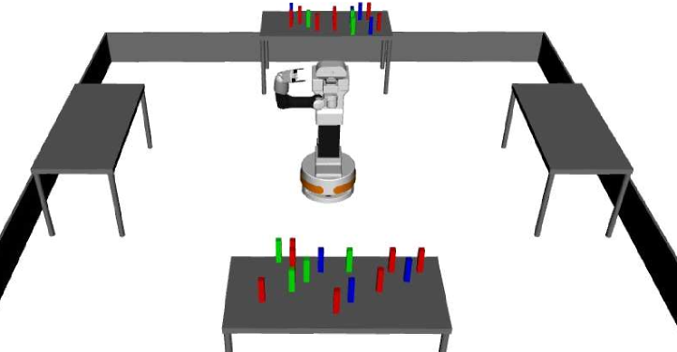
Providing reasoning capabilities to embodied agents so that they are able to solve complex tasks that involve physical interaction with their environment is a long-pursued challenge. By achieving this goal, the humanity would be closer to benefit from autonomous robotic companions to help in a huge variety of tasks. These capabilities can be developed from planning perspective, in which the agent(s) must take into account symbolic and geometric reasoning to decide what sequence of actions should be taken to solve a given task. This kind of problems are known as combined task and motion planning, CTMP (10.3389/frobt.2021.637888). In order to solve CTMP problems (see some examples in Figure 1), two challenges must be addressed (doi:10.1146/annurev-control-091420-084139): for the task-planning part, solving which sequence of symbolic actions must be followed; and, for the motion-planning part, satisfying the geometric constrains that must be met for each action needs to be addressed (alma991002669209706711). However, these two challenges are not independent and must be addressed together. Therefore, it is crucial to find a decision-making process that tackles the CTMP problem in an integrated fashion and minimizing the overall algorithm run-time.

Refer to caption — Figure 1: Example instances of CTMP benchmarking problems: *Sorting Objects* (top) and *Non-Monotonic* (bottom).

The most consuming operation of the algorithm is checking the geometric feasibility of a plan. Therefore, CTMP approaches can be categorized according to how they combine the plan construction with the expensive validity checks. Then, there are three main strategies: sequence-before-satisfy (bidot_geometric_2017), in which the symbolic action sequence is found first, and continuous parameter values are then searched in order to meet the geometric constrains; satisfy-before-sequence (7733599), in which the geometric problem is solved first to find sets of satisfying assignments for individual constraints and, afterwards,action sequences that use those values are searched; and, interleaved (doi:10.1146/annurev-control-091420-084139; cambon_hybrid_2009), in which actions are added to the action sequence (i.e. the plan) and constraints are satisfied progressively.

The proposed approach is framed in the interleaved strategy. However, for when to compute the constraint satisfaction, there are also a variety of options. These can range from doing this calculation for each action to be considered, to making partial plans and then verifying if there is a solution to the constraint satisfaction for the whole subplan. Furthermore, lazy approaches can be considered (dornhege_lazy_nodate; dellin_unifying_2016). On this kind of strategies, a relaxed version of the geometric problem is solved more frequently (e.g. for each action) and then a complete version is solved, as a final check, significantly less frequently (e.g. when a subplan is found). This work follows this strategy, referred here as the lazy approach.

Also, CTMP approaches can be classified according to whether the state variables are pre-discretized (FerrerMestres2017CombinedTA) or sampled within the search (Thomason). In this work, the state variables are sampled using and adaptative strategy to efficiently build the search-space from the physical world.

Nevertheless, in the robotics field, often it is hard or even unfeasible to model both the world (states), the actions and the goal(s) in a symbolic and declarative fashion (i.e. specifying symbolic pre- and post-conditions, costs and effects). Indeed, only after applying the action in a digital twin an accurate-enough result estimation can be retrieved. This precludes the use of guides or heuristics associated with this type of information like, for instance, the heuristics proposed by Bonet and Geffner (BONET20015) or the one proposed by Hoffman and Nebel (article). Thus, other type of efficient algorithms that can work with the state and goal structures only, such as width-based search algorithms, should be used (Lipovetzky2014WidthbasedAF; Lipovetzky2021WidthBasedAF). Width-based search algorithms exploit the fact that classical-planning problems can be characterized in terms of a width measure that is bounded and small for most planning domains when goals are restricted to single atoms. The developed framework leverages width-based search algorithms and is able to work directly on states belonging to continuous domains through a simulator. In this way, it works transparently on real variables typical of robot environments. In addition, it works with actions that correspond directly to valid robot operations (e.g. movement plans associated with picking up an object). Furthermore, again from a black-box perspective, it is only possible to query whether a state is a goal or not.

CTMP problems usually involve complex tasks that imply large action plans, which are hard to find. However, the fact that most of these problems contain conjunctive goals can be exploited and, hence, they can be decomposed in single-goal subproblems. Within the width-base search approach, algorithms like, Serialized Iterated Width, SIW (Lipovetzky2014WidthbasedAF), tackle in a serialized way each of the conjunctive goals (i.e. one at a time). However, knowing how the goals should be serialized is not trivial. This issue can be solved combining SIW with policy sketches, $\text{SIW}_{R}$ , which allow expressing domain knowledge by turning it into rules used to decompose the problem (Drexler2021ExpressingAE). The proposed approach integrates this strategy to speed up the search.

Search Algorithm

The proposed search algorithm, called Lazy-SIW_R, is based on the SIW_R algorithm (Drexler2021ExpressingAE), since it can tackle huge search-spaces and multi-goal problems and work with actions whose applicability, effect, and cost is given by a black box (e.g. a simulator). Nevertheless, SIW_R is extended here to be able to work efficiently with a lazy action-validation, i.e. performing a relaxed action-validation within the search and a complete validation when a potential plan is found.

Lazy-SIW_R

Similarly to the regular SIW_R, the proposed algorithm takes as input a start state, a function checking if a given state is a goal state and a policy sketch (see Algorithm LABEL:alg:LazySIW_R). In order to solve a problem, Lazy-SIW_R iteratively selects the next subgoal based on the provided sketch, solves the subproblem and concatenates the subplans, until the final goal is reached (if a solution exists). Differently from SIW_R, the new algorithm uses a novel version of the algorithm IW (lipovetzky-geffner-ecai2012) that supports lazy action-validation and has been consequently named Lazy-IW. Notice that, although Lazy-IW lazy validates the actions during a subplan candidate, the subplan returned to Lazy-SIW_R is completely valid (i.e. has been non-lazily checked).

Lazy-IW

Outlined in Algorithm LABEL:alg:LazyIW, it consists of a series of $k$ -width searches IW $(k)$ , for increasing values of $k$ until the problem is solved or $k$ exceeds the number of problem variables (i.e. a solution does not exist). In order to implement the novelty-based pruning, a novelty table must be maintained, in which the atom tuples discovered during the search are stored. Nevertheless, in the lazy approach, the connections between the discovered nodes are provisional until its final validation during the plan checking. This implies, that a certain node (and, potentially, its successors) could lose its connection to the root node and thus not be an accessible state anymore. Then, if the node resulted to be inaccessible, the atom tuples introduced by the node should not have been taken into account in the search process. In addition to correcting the novelty table, some pruned nodes -stored without duplication in the $pruned$ list (Lines 2 and 16 of Algorithm LABEL:alg:LazyIW)- will need to be recovered and explored, since these tuples could have mistakenly caused their pruning (as they were later discovered but providing the same tuples). Note that the stored pruned nodes, are still updated when rediscovered, updating their parent list (Lines 17-18 of Algorithm LABEL:alg:LazyIW). This implies changes in the novelty-table structure and in the algorithm itself, with respect to the original IW.

In particular, the novelty table, besides containing the tuples seen so far within the search, contains here information about the node that originated that tuple for the first time, as well as the nodes that would have also provided that tuple if the pioneer node would not have been discovered. Note that these non-pioneer nodes need not have been pruned since they could have provided any other novelty that would have ensured their survival. Therefore, in the case of non-lazily checking the actions of a potential plan and a node across the plan becoming orphan (i.e. it loses the connection to root because a movement planning has failed), the novelty table is repaired (see Figure LABEL:fig:novelty). This implies taking into account the tuples that the orphan node originated but also those tuples originated by the successors that have also become orphans -not all the successors became orphans, since they can have another genealogical branch still connected to root. Those tuples contributed only by the now-orphan nodes, must be deleted from the novelty table, leaving the novelty table as if those nodes had never been seen (because they are really not accessible from the root node). Furthermore, in the event that nodes had been discovered that also generated the affected tuples but had been pruned upon discovery for that very reason (Lines 25-26 at Algorithm LABEL:alg:LazyIW), these nodes (and their successive descendant nodes) are inserted in front of the $open$ queue (Line 11 at Algorithm LABEL:alg:GetPlan), to give the tree a chance to achieve the state it would have reached if the orphan nodes had never been seen (i.e. as if all the actions had been checked in a non-lazy way).

In the original algorithm, each node has only one single parent, even when a node is reachable from other nodes (the parent node to be imposed is the one encountered first). Keeping only one parent node for each node, without checking if this connection is really valid, entails a number of problems. For example, if the connection between a parent and its successor is finally checked to be invalid, the child node and all its successors would be disconnected from the root node. Dropping all these nodes could make the problem solution to be completely inaccessible, leading to the failure of the algorithm. In order to mitigate this problem, another two mechanisms have been designed.

On the one hand, in the proposed approach, nodes are allowed to have more than one parent. In this sense, when an already discovered node is found, this new parent-child relationship is established with the node that is already kept in memory (i.e. in $open$ or $closed$ ). This operation can be found at Lines 7-12 of Algorithm LABEL:alg:LazyIW. Nevertheless, the node parents are ordered in increasing order of cumulative cost (i.e. the addition of the edge cost to the cumulative cost of the parent) and only the better parent acts as such, to encourage cheaper (i.e. better) solutions. Thus, when a potential plan is under complete validation, if a certain edge is dropped (i.e. the edge was not really valid), a node gets disconnected from its main parent. Then, the following parent node takes the place of the main one and the plan validation follows (see Figure LABEL:fig:multiparent). This process is repeated until a confirmed parent is found or there are no more parent candidates available at this moment. This mechanism can be found at Lines 10-13 from Algorithm LABEL:alg:GetPlan. In both scenarios, the cost to reach the node from the root node could have changed, either because the new parent offers a higher cost or either because the node is now orphan (i.e. no more parents are available), setting its cost to infinite in this case. Also, notice that if the given node changes its cumulative cost, the cost of its successors (and the successors of the successors and so on) must be also updated according the new node cost. In the original algorithm, nodes have no information of their successors (only their parent), therefore, in order to be able to make the appropriate cost updates in this version of the algorithm, the nodes are doubly linked, meaning that the nodes keep pointers to its parents and also to its successors. This linking operation is performed at Lines 9, 12, 18 and 21 of Algorithm LABEL:alg:LazyIW.

On the other hand, the last mechanism that has been developed to mitigate the side effects of the lazy approach is keeping in memory (i.e. in the $closed$ list) the chains of nodes that are connected to a goal node, but its connection to the root node was dropped during a non-lazy validation process. These chains are formed during a plan validation when the goal ancestors are tried to be validated non-lazily. Each time this validation is successful, the validated node is marked as connected to goal (as it can bee seen at Line 7 of Algorithm LABEL:alg:GetPlan). Then, if any of the nodes of this chain is rediscovered during the search (i.e. a potential parent connected to the root node exists), the search is interrupted since a potential solution has been found. This can be found at Lines 13-15 of Algorithm LABEL:alg:LazyIW. In this case, the plan between the rediscovered node and its connected goal was already validated and only is left the validation between the root and the rediscovered node (see Figure LABEL:fig:orphan). Thus, by means of this re-wiring mechanism, chains of nodes (and all the computations needed to form find it) can be reused.

CTMP for Mobile Manipulation

The proposed approach works with continuous variables that capture aspects from the physical world by drawing a finite number of samples to build the search space. Notice that not all actions may be valid due to geometric constraints and that their feasibility, as well as their cost and effects, is not known a priori (only when trying to plan them in the simulator).

Action validation

Actions involving interaction between the robot and its environment require a validation process to verify that the robot movement is feasible. For this, there must be a trajectory in the robot joint-space that respects its movement capabilities and does not involve self-collisions nor collisions with the environment. Here, the general framework MoveIt! (moveit) is used, although this work is framework-agnostic, to simultaneously map the actions to a real and valid robot motion and validate them, checking sequentially the following functions:

1.

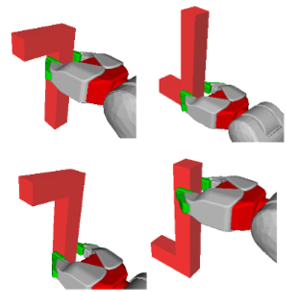
InArmWorkspace: Returns $\mathrm{true}$ when a given target (e.g. an object to interact with) is within the robot arm’s reach, and $\mathrm{false}$ otherwise (see Figure 2(c)).
2.

InverseKinematics: Returns $\mathrm{true}$ only when a valid non-collision robot joint configuration is found, to place the robot gripper at a target (see Figure 2(d)), using a general robot-agnostic iterative Inverse Kinematics (IK) solver algorithm (IK). Notice that if the target is not within the arm workspace, i.e. InArmWorkspace fails, an IK solution does not exist and, then, InverseKinematics will fail after a timeout.
3.

MotionPlan: Returns $\mathrm{true}$ only when a valid motion plan is found, to place the robot gripper in a target and perform the corresponding action (see Figure 2(e)), using a motion-planning algorithm, e.g. RRT-Connect (RRTConnect). Note that if there is no valid robot configuration to grasp an object, i.e. InverseKinematics fails, a motion-plan solution does not exist and, hence, MotionPlan will fail after a timeout.

In the traditional approach (i.e. non-lazy), all these three steps are all checked before considering that an action is valid. Nevertheless, in the proposed approach, only the first two steps are verified when checking the actions in a lazy fashion (as they are fast to compute), while the third step is only verified when checking the actions in a non-lazy fashion (to invest time only in fully-checking those actions that are part of a potential solution plan). Note that the introduced validation-pipeline refers only to manipulation actions. For other cases, other validation steps may be required.

Experimentation and Implementation

The proposed planning framework has been evaluated on two benchmarking problem families from the set proposed by Lagriffoul et al. (Lagriffoul2018PlatformIndependentBF), in an effort to ease comparison of this work with present and future CTMP approaches (i.e. by using what is intended as a standard specification format and set of benchmarking problems for the field). This benchmarking problem set is independent of specific planners and specific robots to maximize portability to different platforms and support physical testing on available hardware. It is important to remark that fairly benchmarking CTMP planners is still an unsolved challenge since currently, the used standard (nor any other) has not reached enough popularity and only few works have reported results in some of the proposed problems.

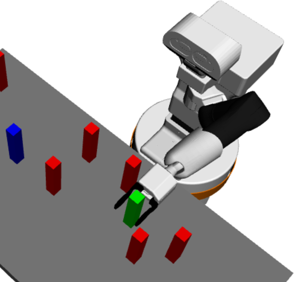
The selected problems, depicted in Figure 1, imply pick-and-place actions in cluttered scenarios (rosell_planning_2019):

•

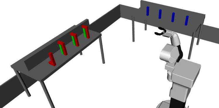
Sorting Objects: A robot must arrange different objects standing on different tables, based on their color. The goal constraints are that all $N$ blue blocks must be on the left table and all $N$ green blocks must be on the right table. There are also $2N$ red blocks, acting as obstacles for reaching blue and green blocks, whose goal position is free. The robot is allowed to freely navigate around the tables, while keeping within the arena, picking and placing the blocks at the tables. The proximity between the blocks forces the planner to carefully order the operations, as well as to move red blocks out of the way without creating new obstructions (i.e. blocking objects). Therefore, solving the problem requires to move many objects, sometimes multiple times (i.e. large task-space).
•

Non-Monotonic: A robot must move $3$ green blocks standing on a table to their corresponding goal position on another table. At the initial state, there are $4$ red blocks obstructing the direct grasp of the green blocks and there are also $4$ blue blocks obstructing the direct placement of the green blocks at their target position. Nevertheless, in this case, the red and blue blocks must end up being at the very same initial locations. The robot is allowed to freely navigate around the tables, while keeping within the arena, picking and placing the blocks at the tables. The goal condition of blue and red blocks requires to temporarily move them away and bring them back later on (non-monotonicity), in order to solve the problem.

The selected problems are a good and broad representation of the challenges currently faced by the state of the art since they involve the following difficulties:

•

Infeasible task actions: Some task actions are unfeasible, i.e. no corresponding motion-plan exists, maybe due to blocking objects or kinematic limits of the robot.
•

Large task-spaces: The underlying task planning problem requires a substantial search effort.
•

Motion/Task trade-off: The problem can be solved with less steps if grasps and placements are carefully chosen.
•

Non-monotonicity: Some objects need to be moved more than once for achieving the goal.

The proposed framework makes no assumptions about which particular problem will be addressed. However, this general approach cannot be directly applied to solve a specific problem without implementing the necessary planner components. Hence, the following single implementation is proposed to tackle both benchmarking problem families.

State-Space

The state must completely specify the status of the environment. For the selected benchmarking problems, this implies that the problem state-space $\mathcal{S}$ contains the kinematic configuration of the robot and its location as well as the location of all the movable objects. Notice that no bits of symbolic state are needed here, as no non-geometric actions are involved in the considered problems. This space may be high-dimensional for even moderate numbers of movable objects. In addition, it entails an infinite-state domain that is beyond the scope of classical-planning search techniques. Therefore, in this framework, a sampling module has been developed in which a finite number of samples of continuous variables are drawn to build the search space directly from the physical world. Hence, sufficiently-rich discretization that represents well the continuous problem world is obtained that at the same time is still tractable.

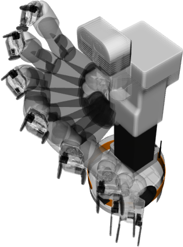
On the one hand, regarding the robot, a single home robot configuration is considered (see Figure 1). Note that this does not imply that the robot cannot move its arm to pick up an object for example (which would make the problem unfeasible), but that the robot starts the pick action with its arm at home and that after picking up the object, the robot returns the arm to its original position (with the object grasped, though). In addition, a predefined number $B>0$ of different robot locations are randomly sampled around the tables (at the start of the search), even if they are initially empty, ensuring that the robot may have access from different locations to any goal position and object standing in any table, not hindering the completeness of the approach hence. The sampled base-locations are roadmapped to define the allowed navigation actions. However, not all the base locations are connected to each other. The maximum travel distance is constrained to a dynamically-computed value. Thus, limiting the connections reduces the number of actions (i.e. the size of the search space). Furthermore, this adds an implicit cost for traveling far which can help to search cheaper solutions without considering the real exact cost of the actions.

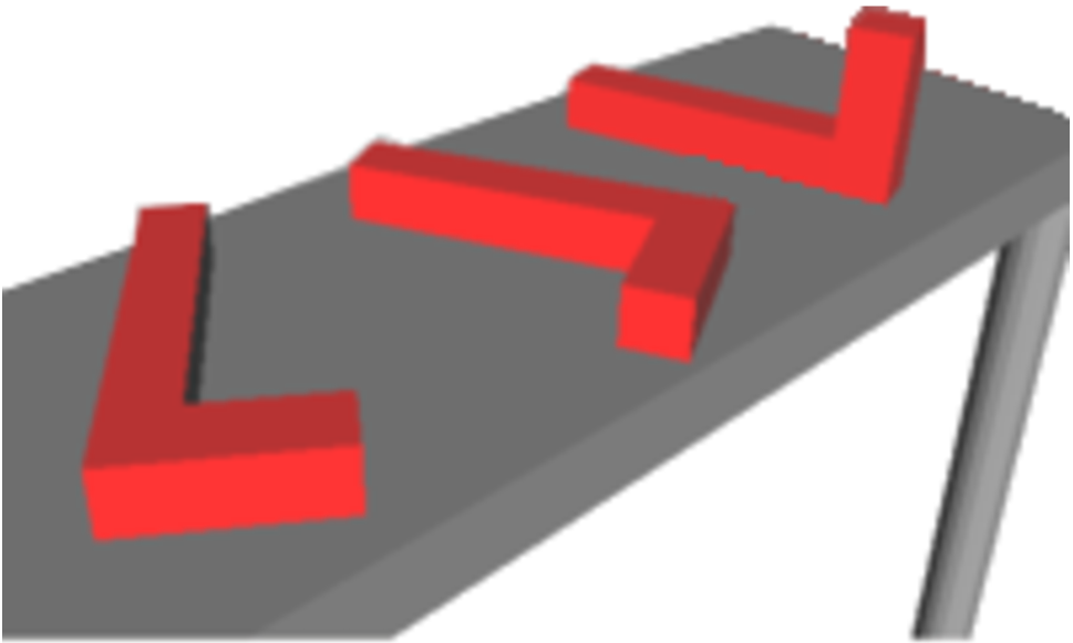
On the other hand, regarding the movable objects (which do not have internal degrees of freedom in the considered problems), a set of $P\geq O$ different allowed object placements (i.e. locations) on the table surfaces are considered simultaneously for the object set, while $G>0$ different grasps and $S>0$ different stable object poses (SOPs) are allowed for each object (see Figure 2). The space of grasps and SOPs, from which to draw samples, is defined in the benchmarking problem specification. However, to obtain the set of placements, an adaptive sampling has been implemented. At the start of every attempt to reach a subgoal, a given number of placements are randomly sampled for each supporting surface (i.e table) in such a way that they are as distant as possible from the other placements, objects and goal positions on that surface. The sampling density of the variables is increased when an attempt to reach a subgoal fails, to obtain new values that can help to find a subproblem solution. This adaptability in sampling and, in particular, the fact that the positions of the objects are continuous, random and not fixed to a templated grid, contributes to having a sufficiently dense sampling (but not denser than necessary) to ensure that the algorithm is complete (i.e. finding solution if it exists). If it were not, for example, by sampling insufficient robot locations, a certain object included in the goal would not be accessible without collisions among the available states. In the same way, it is meaningless to have a density of placements within a supporting surface in which the distance between placements is smaller than the average size of the mobile objects. Otherwise, if a placement is occupied by an object, the robot will not be able to put any object in the neighboring placements because the objects will collide, but the search algorithm ignores this until it tries to perform the action (note that the actions structure is hidden as a black box).

Note that the size of the state-space $\mathcal{S}$ (and, therefore, also the problem complexity) increases exponentially with the number $O$ of movable objects (given by the problem definition), and only polynomially with the sampling parameters (i.e. $B$ , $P$ , $G$ and $S$ ). Notice that the start and the goal states are included in the defined state-space but, nevertheless, that not all the states may be accessible from the initial state.

Action-Space

Actions connect problem states and are the only means by which the robot and objects can change internal state and location. In the selected problems, the action-space $\mathcal{A}$ is restricted to the following parametrized actions:

•

Pick actions that, when valid, allow the robot to pick up, from a given base location, a specific object, which is in a specific pose, using a specific grasp, as long as the robot is not already holding any object.
•

Place actions that, when valid, allow the robot to place a particular object, which must be grasped with a given grasp, in a given placement using a given SOP.
•

Move-Base actions that, when valid, allow the robot to change its location from a given position to a different one, dragging with it the object it might be holding.

The size of the action-space also increases exponentially with the number of movable objects and polynomially with the sampling parameters. Notice that not all actions may be valid due to geometric constraints and that their feasibility, as well as their cost and effects, is not known a priori (only when trying to plan them in the simulator).

Novelty atoms

The proposed approach prunes the discovered states not passing a novelty filter, which operates on atoms factorizing the states. For the considered benchmarking problems, the used atoms are of type robot-at- $p$ and object- $o$ -at- $p$ , for some given poses $p$ and objects $o$ . This definition allows solving the benchmarking problems with a maximum novelty of 1 (as shown in the next Section). Note that, unlike the defined states, these atoms do not capture grasp information (reducing the atom-space size). Then, the number of atoms grows linearly with the number of objects and the sampling parameters.

Sketch rules

The algorithm $\text{SIW}_{R}$ is able to decompose the problem into sequential subproblem using a user-provided domain knowledge, encoded into a set of rules that outline a sketch of the solution. These rules operate on state features that capture relevant information about the problem status. The following features have been implemented:

•

$H$ : a Boolean that equals $\mathrm{true}$ if the robot is holding an object, and $\mathrm{false}$ otherwise.
•

$F$ : a Boolean that equals $\mathrm{true}$ if there exists a goal pose of the grasped object that do not blocks the pick/place of any other misplaced object, and $\mathrm{false}$ otherwise.
•

$m$ : the number of misplaced objects, defined as the objects that are standing (and, hence, not held) outside their associated goal position/region (if the object has no associated goal position, it is never misplaced) or are held and their goal position/region is blocked.
•

$n$ and $s$ : respectively $\min b_{i}+c_{i}$ and $\sum b_{i}$ , with $b_{i}$ being the minimum number of objects blocking the $i$ -th misplaced object (i.e. preventing it from being picked up from its current position and put down in its goal position/region) and $c_{i}$ the minimum number of misplaced object blocked by the goal position(s) of the $i$ -th misplaced object. Note that approximations are used and no inverse kinematics is solved within this computation, to speed up the process. During the search for such a minimum value, it is considered the best robot location and grasp for the pick action and the best robot location, object placement and SOP for the place action in the goal zone, while maintaining consistency (i.e. using the same grasp for the considered pick and place pair).

Using these features, the goal in both family problems is expressed as $\neg H\wedge m=0$ (i.e. the robot is not holding any object and all the objects are at their goal positions). In adition, the following mutually-exclusive sketch rules have been established for both benchmarking problem families:

•

$\{\neg H,\,m>0,\,n=0\}\mapsto\{H,\,F,\,m\!\downarrow,\,n?,\,s?\}$ : active if there is at least one misplaced object ( $m>0$ ) that can be picked up and placed down directly ( $\neg H$ and $n=0$ ), enforcing to pick it up (i.e. lower $m$ and make $H$ true).
•

$\{\neg H,\,m>0,\,n>0\}\mapsto\{H,\,F?,\,m?,\,n?,\,s\!\downarrow\}$ : active if there are still misplaced objects ( $m>0$ ) but they cannot be picked up directly ( $\neg H$ but $n>0$ ), enforcing to pick any obstructing object (i.e. decrement $s$ ). However, $n$ may be accurately estimated, picking an unexpectedly-accessible misplaced object would also satisfy this rule (which is not an inconvenience at all).
•

$\{H,\,F\}\mapsto\{\neg H,\,F?\}$ : active whenever the robot is holding an object, which would not block other misplaced object once placed if it had a goal associated with it, enforcing to place it but not in a wrong position (i.e. do not change $m$ ) and without disturbing the access to the pending misplaced objects (do not change $n$ or $s$ ).
•

$\{H,\,\neg F\}\mapsto\{\neg H,\,F?,\,m?\}$ : active whenever the robot is holding an object that cannot be placed on their goal without blocking any misplaced object, enforcing to place it somewhere else without disturbing the access to the pending misplaced objects (do not change $n$ or $s$ ).

Results and Discussion

The proposed framework has been evaluated in different instances of the selected benchmarking families, to analyze its performance in various environments but also to allow direct comparison with other approaches in the same scenario. The framework has been run in an Intel® Core™ i7-10610U CPU at 1.80 GHz, with 8 processors and 16 Gb of RAM, on Ubuntu 20.04.4 and ROS Noetic, and validated with a TIAGo robot from PAL Robotics (see Figure 1). Videos of the obtained plans can be found in https://drive.google.com/drive/folders/110VtyoSNrw0hjR7Wma7fumqJIB9wxr3L. The results obtained by the proposed approach, together with the ones of some relevant algorithms, can be found in Table LABEL:tab:solution. Non-Lazy and non-goal-serialized versions of the approach have also been tested in these same scenarios as a baseline of the performance improvement provided by each of the proposed strategies. However, the results obtained without using goal-serialization are not included since these planners cannot solve any problem in the allocated time.

All the considered problems have been successfully solved within $1$ h. Note that this budget time, which would not be admissible on a real application, has set intentionally generous to show the soundness and completeness of the algorithm. During the experimentation, the effectiveness of the planner has been demonstrated by not requiring planning times longer than the execution time of the produced plans. Indeed, the proposed approach requires less time to find a solution compared with the results obtained by BFWS (FerrerMestres2017CombinedTA), which also use a width-based algorithm, and Planet (Thomason), which performs normal motion planning in a space including both geometric and symbolic states. Notice that, in order to make a fair comparison, any pre-computation or other planning effort conducted offline are also considered as planning time in Table LABEL:tab:solution. Note that the proposed approach specifically avoids this sort of offline work since, in a real application, there is no guarantee that the objects will be in the positions foreseen in the pre-processing, or that objects of different geometry will not be used.

The planning time depends on both the number of expanded nodes and the required time for expanding each node. Regarding the first factor, even though the problem search-space is huge, the planner manages to find a solution expanding only a minimal fraction for all the problems. Thanks to the used atom features and sketch rules, a novelty of 1 has been enough to solve all the problems. In this way, the underlying IW $(k)$ algorithm applies the maximum level of node-pruning (thus, minimizing the number of expanded nodes). In addition, the generated decomposition in subproblems has efficiently guided the search by obtaining a sequence of subgoals very close to each other (i.e. they require limited exploration to reach them consecutively).

Furthermore, the followed strategy of adaptive sampling allows to use a reduced but useful selection of placements in each subproblem. With fewer placements, the search-space is reduced but, in addition, as the sampled placements are automatically adapted to the specific situation of the subproblem, the subgoals are reached quickly.

The node-expansion time in the proposed approach mostly depends on the geometric validation of each of the actions. This includes three steps (i.e. InArmWorkspace, InverseKinematics and MotionPlan) that act as sequential filters (i.e. if a step fails, the next ones are not computed and the action is set as unfeasible). Note that they act in increasing order of computational load and decreasing order of relative discriminative power (i.e. rejection ratio over the non-filtered actions in the previous step). This permits discarding quickly the majority of unfeasible actions with a very small computational cost (see some illustrative values in Table LABEL:tab:profiling). In addition, decomposing the action-validation enables delaying the computation of the most expensive step (i.e. MotionPlan). Thus, the complete validation is only computed on those actions that are part of a potential plan (i.e. lazy approach). Note that satisfying the InverseKinematics step almost ensures that the action is valid. This is essential to make using the lazy approach advantageous. Indeed, as it can be seen on Table LABEL:tab:solution, following the lazy approach reduces drastically the planning time.

Implementing the lazy-approach, however, implies some challenges. Since the actions are all provisional (until a plan is validated), all the found parents in each node must be kept to prevent discarding connections that are part of the solution. Besides, the planner keeps record on node chains that are connected to a goal but got sometime disconnected from the root node within a plan validation. These two mechanisms are relevant when many nodes need to be expanded in a subsearch. Another important challenge is the adaptation of the IW $(k)$ to keep track of the novelty. Thus, when a provisional action turns to be unfeasible, if the node becomes orphan (i.e. disconnected from the root node), the novelty introduced by this node has to be revised. Solving the different problems has implied the activation of this mechanism in multiple occasions. This has prevented to wrongly prune graph branches that are part of the solution.

Another important metric is the quality of the produced plans. Although optimality can not be formally ensured, the proposed algorithm performs notably on avoiding unhelpful actions (i.e. near-optimal solutions). This is facilitated by the proposed sketch since its rules discourages moving non-misplaced objects that do not block any goal object or goal placement but promotes moving the easier goal-objects first. Hence, after moving these objects, often other goal objects became accessible without needing to move non-goal objects. Indeed, when comparing the results with the other approaches, plans containing fewer actions are obtained for the same problems with the proposed approach.

The proposed algorithm performs well even with a high number of objects and goals. However, high-cluttered problems are challenging. On these problems, the goal objects can be obstructed by many objects, which must be moved away. Nevertheless, there is a limited space where the obstructing objects could be set aside (without blocking other necessary areas). In this scenario, most of the inverse-kinematic computations fail, reaching the timeout. This implies a slower node expansion and a higher difficulty to find valid actions. In addition, as there are so few gaps, the proposed approach samples the placements more densely to ensure that there exists an accessible placement. On the contrary, Planet does not scale well with the number of objects. BFWS scales well, though, but at the cost of rigidity as it pre-compiles and forces the objects to be in a fixed grid distribution during the search process. With this inflexible approach, the planner manages to reuse many inverse-kinematic and motion-planning computation.

Conclusions and Future Work

This work has addressed the problem of planning simultaneously the tasks and movements of robots to solve a given problem where these two issues cannot be tackled in a decoupled manner. Thus, a new framework has been developed, obtaining near-optimal robot plans, quickly and efficiently, even for complex problems. The developed framework includes a width-based search algorithm, implementing a novel lazy-interleaved strategy to reduce the computational cost of the planning, without making any assumption on the robot used or the number, types, locations and geometries of the objects. This efficient approach focuses the motion-planning efforts only in potential solutions, thus, obtaining a fully-online and flexible approach that does not require any pre-computing at all (enabling reactive planning). Besides, domain knowledge provided via sketches has been integrated in the proposed approach, proving to be very effective. The proposed approach works transparently with robotic continuous state-spaces (coming directly from the robotic framework) and with flexibility using an adaptive sampling of the world to build the search space of the problem. This helps maintaining the planner completeness and reduces the sim-to-real gap since it can produce any real location (not only templated positions as grids). Moreover, the problem dynamics are retrieved as a black box, so the developed planner is able to work directly with a simulator, and it does not need an explicit declaration of the action structure. The proposed approach has been validated in problems that characterize the current challenges addressed in the state of the Art. Furthermore, the proposed approach has been compared with state-of-the-art approaches, obtaining significantly better results, mantaining a planning time reasonable with respect to the plan execution time. Finally, the proposed approach has been combined and integrated within the ROS environment in order to provide the highest level of standardization and compatibility with the maximum number of robotic systems currently available.

Nevertheless, there are still several interesting topics that could be treated in future work:

•

Inclusion of learning AI-based techniques to obtain self-learned rules, features and sampling strategies.
•

Extension to consider optimality and being able to tackle problems with state uncertainty and partial observability, where dynamics- or physics-based planning is needed.
•

Post-processing the obtained plans by using optimal motion-planning algorithms, e.g. Informed RRT^∗ (6942976), and merging and shortening the trajectories of consecutive actions.