M³RS: Multi-robot, Multi-objective, and Multi-mode Routing and Scheduling

Abstract

In this paper, we present a novel problem coined multi-robot, multi-objective, and multi-mode routing and scheduling (M³RS). The formulation for M³RS is introduced for time-bound multi-robot, multi-objective routing and scheduling missions where each task has multiple execution modes. Different execution modes have distinct resource consumption, associated execution time, and quality. M³RS assigns the optimal sequence of tasks and the execution modes to each agent. The routes and associated modes depend on user preferences for different objective criteria. The need for M³RS comes from multi-robot applications in which a trade-off between multiple criteria arises from different task execution modes. We use M³RS for the application of multi-robot disinfection in public locations. The objectives considered for disinfection application are disinfection quality and number of tasks completed. A mixed-integer linear programming model is proposed for M³RS. Then, a time-efficient column generation scheme is presented to tackle the issue of computation times for larger problem instances. The advantage of using multiple modes over fixed execution mode is demonstrated using experiments on synthetic data. The results suggest that M³RS provides flexibility to the user in terms of available solutions and performs well in joint performance metrics. The application of the proposed problem is shown for a team of disinfection robots. The videos for the experiments are available on the project website.

I Introduction

Multi-robot teams are being widely used to address complex tasks such as manufacturing [1], disaster response [2], logistics [3], and many more. Multi-robot task allocation algorithms (MRTA) [4, 5] allocate tasks to various robots working on a common mission while optimizing a joint objective like completing tasks in time. Many real-world applications of multi-robot teams dictate the optimization of multiple factors (or objectives), which could be conflicting. In such cases, a multi-objective optimization framework is adopted for MRTA, where multiple solutions are generated to explore trade-offs between different objectives. Several works have explored trade-offs for multi-objective MRTA like task performance vs communication throughput [6, 7], reduced resource consumption vs performance [8], or completion times vs total travel length [9]. In such cases, the task allocations are altered to achieve different trade-offs. However, the current literature does not explore using distinct task execution modes to address different trade-offs arising in multi-robot missions.

Task execution modes refer to different operational settings in which a robot can perform a task. The usage of different modes is dependent on various constraints arising in the environment or to achieve desired performance on key metrics like quality and resource consumption. Task execution modes have been used in the context of single robots to prioritize different goals. Lahijanian et al. [8] explores the usage of energy-saving mode where resource-intensive autonomy features are disabled to save energy for navigation in a resource-constrained environment. Chen et al. [10] considered applications where robots can switch between automated and manual driving modes based on the environment. The task execution modes of individual robots in a multi-robot mission can impact various metrics of the mission, like quality of task execution, quantity of tasks completed, and timeliness of robots. Hojda presents a routing and scheduling algorithm with task execution modes for multi-robot systems [11]; however, they only considered minimization of resource consumption as the objective. Using individual robot-level task execution modes for MRTA problems with multiple objectives remains unexplored.

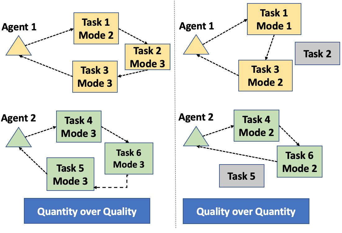
Figure 1: M³RS is suitable for routing and scheduling in time-bound scenarios where multiple criteria of interest depend on the mode in which the agents execute the tasks. This visualization depicts two cases. Here, mode 1 stands for the highest quality and long task execution times, whereas mode 3 is for the lowest quality and fastest task execution times. The left side of the image shows a case where agents choose to maximize the number of tasks completed by performing tasks in lower-quality modes. On the right, agents prioritize quality over quantity. As a result, tasks 2 and 5 are missed. An example of such a scenario is a multi-robot system performing services such as cleaning.

To the best of our knowledge, this is the first work that deals with the selection from multiple task execution modes for multi-objective multi-robot routing and scheduling. The goal of M³RS is to assign tasks to robots that can be executed in different modes. The proposed formulation is well-suited for applications where tasks are spread across a physical space, each task has service requirements and resource requirements, and the overall mission has multiple criteria of interest. Each robot can address the task in multiple execution modes, where each mode corresponds to different task quality, resource consumption, and service times. A visual depiction of the application of M³RS is given in Fig. 1. We present a mixed linear integer programming formulation for the proposed problem. The optimization formulation becomes computationally intensive for larger problem instances. A column generation method addresses the challenges of increasing computation time for larger problem instances. We showcase the utility of M³RS for a multi-robot disinfection mission. We implemented M³RS for a real-world experiment for a team of disinfection called G-robots [12]. While we present results for multi-robot disinfection applications, the M³RS formulation can be extended to other applications.

This paper is organized as follows: Section II reviews relevant literature. The general formulation and optimization of M³RS is given in Section III. The results of the synthetic, simulated, and real-world experiments are presented in Section IV. Finally, Section V includes future works and conclusions.

II Literature Review

MRTA with multiple objectives creates a set of solutions of task assignment for robots in applications with multiple factors (or objectives) of interest. Each solution represents a certain trade-off between multiple desired objectives. Many works in literature have addressed multi-objective MRTA for distinct situations. Flushing et al. [6] optimized task allocation in a multi-robot team for two objectives of task performance and communication throughput of the team. In [7], the allocation for a team of drones used a trade-off between quality of communication and area coverage for a surveillance application. A trade-off between minimizing wait times and avoiding foot traffic for a multi-robot pick-up and delivery application was explored in [13]. Many routing-based MRTA explored minimizing multiple objectives like makespan, maximum distance traveled, and distance traveled per robot [14, 15]. In [16], a trade-off between task productivity and human operator fatigue was considered for collaborative human-robot tasks. Most of the aforementioned works address distinct trade-offs by varying the ordering or assignment of tasks to be executed. They don’t consider the trade-offs arising from distinct task execution modes.

Usage of task execution modes in the context of MRTA is still unexplored. In [17, 18], task assignment formulation with execution modes for human-robot collaboration in work cells was presented. These models assigned different collaborative modes for the execution of a task. The collaborative modes can include joint execution of tasks by human workers and a robot or independent execution by human workers/robots. However, the models developed in these works only consider static robots working in an assembly cell. In contrast, M³RS considers mobile robots that must visit different locations to execute the tasks. Furthermore, in our case, task execution modes are different ways in which an individual agent can perform the task.

The application of modes has been addressed in routing and scheduling literature. Resource-constrained project scheduling (RCPS) is an important problem in operation research for scheduling resources to perform different activities [19]. The typical formulation minimizes the total makespan of the project while adhering to metrics such as resource capacities and precedence constraints. An important variant of RCPS accounts for having multiple task execution modes [20, 21]. However, these models don’t consider the transportation or routing of agents. Task execution modes and routing for multi-agent systems were addressed in [11]. They presented a formulation that generates routes of agents to complete tasks and the corresponding execution modes. However, their formulation only considers the minimization of resource consumption as the objective. In such cases, the optimization model defaults to selecting modes with minimum resource consumption. In contrast, we consider trade-offs arising due to the selection of different modes in our optimization model.

A flavor of mode selection is found in vehicle routing problems with delivery options [22]. In such problems, customers have multiple possible delivery locations (called options), and each delivery location has constraints, such as capacity or time windows. In their case, the selection of different options/modes impacts the target delivery location for a customer. Another variant of a hybrid electric vehicle routing problem with mode selection is presented in [23]. They used a mode selection mechanism for switching between different driving modes of hybrid vehicles while going from one customer to another. Different driving modes have an impact on emissions and costs associated with transportation.

III Multi-Robot Multi-Objective Multi-Mode Routing and Scheduling

In this section, first, the general optimization model for M³RS is presented. Then, the formulation for multi-robot disinfection is discussed. Finally, a column generation scheme to solve the optimization model with faster computation time is given.

Table I: Notation for M³RS

Notation	Description
$\mathcal{A}$	Set of agents.
$\mathcal{T}$	Set of tasks.
$\mathcal{M}_{i}$	Set of modes for task $i$, where $\mathcal{M}_{i}=\{1,2...M\}$.
$R$	number of objective criteria.
$f_{r}$	$r^{th}$ objective criterion.
$p_{i,m}$	The cost of task $i$ in mode $m$.
$\sigma_{i,m}$	Time to complete task $i$ in mode $m$.
$d_{i\scriptsize{\xrightarrow{}}j}$	Energy consumed for travelling from tasks $i$ to task $j$.
$d_{i,m}$	Energy consumption of task $i$ in mode $m$.
$[a_{i},b_{i}]$	Start and end time for task $i$.
$Q$	Total capacity of an agent.
$T_{H}$	Time available to complete all tasks.
$t_{i,j}$	Travel time from task $i$ to task $j$.
$\lambda_{r}$	The scalar preference for $r^{th}$ objective function.
$s^{k}_{i}$	A decision variable for arrival time of agent $k$ to task $i$.
$x^{k}_{i\scriptsize{\xrightarrow{}}j}$	A binary decision variable for if agent $k$ goes from task $i$ to task $j$.
$y^{k}_{i,m}$	A binary decision variable for task $i$ done in mode $m$ by agent $k$.

III-A Optimization Model

M³RS solves routing and scheduling problem for a set of agents $\mathcal{A}$, and a set of tasks $\mathcal{T}$ spread across a physical space. All the agents are identical, and only one agent can service each task. We use $i$ and $j$ to denote different tasks in $\mathcal{T}$ and $k$ to denote $k^{th}$ agent to describe the rest of the notation. Each agent has a limited energy budget or capacity given by $Q$. The energy required to travel from task $i$ to task $j$ is given by $d_{i\scriptsize{\xrightarrow{}}j}$. The time window for a task specifies a starting time ($a_{i}$) and finishing time ($b_{i}$) within which the task must be serviced. The entire multi-robot operation must be done in a fixed mission time of $T_{H}$ hours. Further, each task has an associated mode set $\mathcal{M}_{i}=\{1,2...M\}$, representing available task service modes. Each task can have distinct modes of service available, so each task has a distinct mode set. An agent services the task in one of the modes available in the associated mode set. The selected mode $m\in\mathcal{M}_{i}$ has an associated service time ($\sigma_{i,m}$) and resources requirement ($d_{i,m}$) from the agent. Performing a task in a mode with higher service time and resource consumption would lead to lower availability of agents for other tasks. The overall scheduling and allocation mission is optimized for multiple objectives. The relevant notation for the formulation is summarised in Table I.

The formulation for M³RS is expressed as a mixed integer linear program to determine for all agent, tasks and modes i) the assignment and transition of agent $k$ from task $i$ to $j$ denoted by binary decision variable $x^{k}_{i\scriptsize{\xrightarrow{}}j}$; ii) execution of task $i$ in mode $m$ for agent $k$ denoted by binary variable $y^{k}_{i,m}$; and iii) arrival time of agent $k$ to task $i$ denoted by a real variable $s^{k}_{i}$. The optimization problem is expressed as:

$$\underset{x^{k}_{i\scriptsize{\xrightarrow{}}j},y^{k}_{i,m},s^{k}_{i}}{\max}\,\sum_{r=0}^{R}\sum_{k\in\mathcal{A}}\sum_{i\in\mathcal{T}}\sum_{j\in\mathcal{T}}\sum_{m\in\mathcal{M}_{i}}\lambda_{r}\cdot f_{r}(x^{k}_{i\scriptsize{\xrightarrow{}}j},y^{k}_{i,m},s^{k}_{i}),$$ (1)

subject to the constraints in Eq (2)-(15).

Eq. (1) is the scalar objective function that maximizes the convex combination of $R$ objective criteria. The user-specified parameter $\lambda_{r}$ represents trade-off preference for $r^{th}$ objective criterion. Each objective criterion can depend on task allocation, selected mode, and arrival times.

The constraints of the optimization (Eq (2)-(15)) are described next. The task assignment constraint is given by:

$$\sum_{k\in\mathcal{A}}\sum_{j\in\mathcal{T}}x^{k}_{i\scriptsize{\xrightarrow{}}j}\,\leq\,1\,\,\,\forall i\in\mathcal{T},$$ (2)

The constraints in Eq. (2) ensure that each task is done at most once. The next set of constraints are flow constraints to eliminate infeasible solutions:

$$x^{k}_{i\scriptsize{\xrightarrow{}}i}\,=\,0\,\,\forall k\in\mathcal{A}\,\,\forall i\in\mathcal{T},$$ (3)

$$\sum_{i\in\mathcal{T}}x^{k}_{i\scriptsize{\xrightarrow{}}0}\,=\,1\,\,\,\forall k\in\mathcal{A},$$ (4)

$$\sum_{j\in\mathcal{T}}x^{k}_{0\scriptsize{\xrightarrow{}}j}\,=\,1\,\,\,\forall k\in\mathcal{A},$$ (5)

$$\sum_{i\in\mathcal{T}}x^{k}_{i\scriptsize{\xrightarrow{}}h}-\sum_{j\in\mathcal{T}}x^{k}_{h\scriptsize{\xrightarrow{}}j}\,=\,0\,\,\,\forall h\in\mathcal{T},\,\,\forall k\in\mathcal{A},$$ (6)

$$\sum_{k\in\mathcal{A}}\sum_{m\in\mathcal{M}_{i}}y^{k}_{i,m}\,=\,1\,\,\forall i\in\mathcal{T},$$ (7)

The constraint in Eq. (3) eliminates infeasible solutions where an agent transitions between the same task. This ensures that all agents leave the home depot and return to the home depot, respectively. The constraints in Eq. (4)-(5) are used. It should be noted that task $i=0$ is considered the home position or starting point for the agent. The constraint in Eq. (6) ensures that the agent must exit the tasks they visit. The constraint in Eq. (7) assures that each task is assigned to one agent, and for each task, one mode is selected. The next set of constraints are mission constraints to enforce capacity and timing-related constraints:

$$\sum_{i\in\mathcal{T}}\sum_{j\in\mathcal{T}}(\sum_{m\in\mathcal{M}_{i}}(d_{i,m}\cdot y^{k}_{i,m})+d_{i\scriptsize{\xrightarrow{}}j})\cdot x^{k}_{i\scriptsize{\xrightarrow{}}j}\,\leq\,Q\,\,\,\forall k\in\mathcal{A},$$ (8)

$$s^{k}_{i}+\sum_{m\in\mathcal{M}_{i}}\sigma_{i,m}\cdot y^{k}_{i,m}+t_{i,j}-s^{k}_{j}\leq 0\,\,\forall i\in\mathcal{T}$$ (9)

$$\forall j\in\mathcal{T}\,\,\forall k\in\mathcal{A},$$

$$a_{i}\leq s^{k}_{i}<b_{i}-\sum_{m\in\mathcal{M}_{i}}\sigma_{i,m}\cdot y^{k}_{i,m}\,\,\,\forall i\in\mathcal{T},\,\,\forall k\in\mathcal{A},$$ (10)

$$0\leq s^{k}_{0}<T\,\,\forall k\in\mathcal{A},$$ (11)

The constraint in Eq. (8) ensures that the agent has sufficient capacity to complete the tasks and travel between different locations. The constraint in Eq. (9) ensures that the arrival time for a subsequent task is always later than the previous task. This constraint also enables sub-tour elimination [24], where sub-tours are infeasible solutions that represent disjoint sequences of completing tasks for the same agent. The Eq. (10) ensures that the agent arrives and completes the task within the prescribed time window of the task. The Eq. (11) ensures that all agents return to the depot within the specified time horizon $T_{H}$. The constraints Eq. (12)-(13) ensure that the variables $x^{k}_{i\scriptsize{\xrightarrow{}}j}$ and $y^{k}_{i,m}$ are binary:

$$x^{k}_{i\scriptsize{\xrightarrow{}}j}=\{0,1\},$$ (12)

$$y^{k}_{i,m}=\{0,1\},$$ (13)

The user preference constraints are given by:

$$0<\lambda_{r}\leq 1,$$ (14)

$$\sum_{r=0}^{R}\lambda_{r}=1.$$ (15)

The constraints Eq. (14)-(15) enforces convexity for the given user preferences.

III-B M³RS for Multi-Robot Disinfection

A fleet of disinfection robots [12] is deployed to complete a disinfection mission. A mission is a collection of disinfection tasks spread in an environment such as a hospital. Each mission has a specified time horizon within which it should be completed. Further, the tasks must be done in their specified time window. The tasks can have different disinfection dose requirements. This dosage dictates disinfection quality, energy consumption, and a robot’s time on a task. Each task can be disinfected in a particular set of modes, where the modes have different disinfection dosage options for that task. We consider four disinfection modes that are $D_{99.9999}$, $D_{99.99}$, $D_{99}$, and $D_{90}$. Here, $D_{99.9999}$ is the strongest disinfection dose with the highest disinfection time and energy consumption as compared to $D_{90}$ [25]. The set of modes can be determined by the acceptable disinfection levels for a surface. So, each task has an associated set of acceptable disinfect doses or modes. The assignment of robots to different tasks and the corresponding modes will be determined by solving M³RS.

For the disinfection applications, we have two objectives: i) number of tasks completed and ii) overall disinfection quality. There exists a trade-off between these two metrics. Higher disinfection quality requires more disinfection time and resources, which limits the availability of time and resources for other tasks. For example, attempting to disinfect with the highest dosage may limit the number of tasks completed in case of a tight mission time. Our formulation creates schedules by using user-specified trade-off requirements. The formulation of M³RS for disinfection application is:

$$\underset{x^{k}_{i\scriptsize{\xrightarrow{}}j},y^{k}_{i,m}}{\max}\,\sum_{k\in\mathcal{A}}\sum_{i\in\mathcal{T}}\sum_{j\in\mathcal{T}}\sum_{m\in\mathcal{M}_{i}}(\lambda)\cdot x^{k}_{i\scriptsize{\xrightarrow{}}j}+(1-\lambda)\cdot p_{i,m}\cdot y^{k}_{i,m,}$$ (16)

subject to constrains in Eq. (2)-(15). Here, $p_{i,m}$ indicates quality of disinfection when completing task $i$ in mode $m$. This mixed integer optimization model can be solved using a standard branch and cut algorithm. However, for larger problem instances, the branch and cut solution has an exploding computation time Next, we present a column generation method to solve M³RS with faster computation times.

III-C A Solution for M³RS: Column Generation

The mixed integer programming formulation of M³RS will have a large computation time with an increase in the number of tasks and the number of robots. We use the column generation [26, 27] to address computational challenges associated with large decision variables of the proposed formulation. The column generation algorithm decomposes the original optimization problem into a master problem and a sub-problem. The master problem identifies optimal columns (or paths/solutions) from a pool of feasible candidate solutions, $\Omega$. Since $\Omega$ is very large, typically, a restricted master problem is solved on a subset $\Omega^{\prime}\subset\Omega$. The sub-problem uses the dual solution from the master problem to find new favorable columns, which are added to $\Omega^{\prime}$ to improve the objective value of the master problem. The master problem and sub-problem are solved iteratively until there are no new columns with positive reduced cost.

For solving the restricted master problem, a set-covering problem formulation is adopted [26]. A set-covering problem selects a subset of variables from a given set. The restricted master problem finds optimal solutions from a subset of feasible candidate solutions $\Omega^{\prime}$. Each candidate in $\Omega^{\prime}$ is a feasible solution that specifies a sequence of addressing different tasks in the associated modes and arrival times. The pool $\Omega^{\prime}$ can be initialized by some trivial solutions and can be updated iteratively with better solutions from the sub-problem. The restricted master problem is given by:

$$\underset{\theta^{k}}{\max}\,\sum_{k\in\Omega^{\prime}}c_{k}\cdot\theta^{k}$$ (17)

subject to:

$$\sum_{k\in\Omega^{\prime}}a^{k}_{i}\cdot\theta^{k}\leq 1\,\,\forall i\in\mathcal{T}/\{0\}$$ (18)

$$\sum_{k\in\Omega^{\prime}}\theta^{k}\leq|\mathcal{A}|$$ (19)

$$\theta^{k}\geq 0$$ (20)

Here, $\theta^{k}$ is the solution selection variable. It simply indicates whether solution k in $\Omega^{\prime}$ is selected. Ideally, $\theta^{k}$ is a binary variable, where it is 1 if the solution $k\in\Omega^{\prime}$ is selected and zero otherwise. However, we use a linear relaxation of restricted master problem where $\theta^{k}$ is relaxed to have real values in the interval [0,1] through Eq. (17)-(20). This enables faster solution computation. The objective function in Eq. (17) selects the schedules from $\Omega^{\prime}$ that maximizes the original objective function Eq. (16). The constraint Eq. (18) ensures that each task is assigned at most once. Here, $a^{k}_{i}$ is 1 if $i^{th}$ task is covered in $k^{th}$ solution. Finally, Eq. (19) ensures the number of candidates selected from $\Omega^{\prime}$ don’t exceed the number of available agents.

The sub-problem generates new columns based on the dual solution of the restricted master problem. We solve a modified version of the original optimization problem as the sub-problem. The sub-problem deals with a restricted set of tasks $\mathcal{T}^{\prime}$ and solves for a single robot. These modifications enable faster computation of candidate solutions. The formulation for sub-problem is

$$\underset{x_{i\scriptsize{\xrightarrow{}}j},y_{i,m}}{\max}\,\sum_{i\in\mathcal{T}^{\prime}}\sum_{j\in\mathcal{T}^{\prime}}\sum_{m\in\mathcal{M}_{i}}(\lambda)\cdot x_{i\scriptsize{\xrightarrow{}}j}+(1-\lambda)\cdot p_{i,m}\cdot y_{i,m}-$$ (21)

$$\sum_{i\in\mathcal{T}^{\prime}/\{0\}}(\gamma_{i}\cdot\sum_{j\in\mathcal{T}^{\prime}}x_{i\scriptsize{\xrightarrow{}}j})$$

subject to constraints Eq. (2)-(15), with $k=0$ and using $\mathcal{T}^{\prime}$ instead of $\mathcal{T}$.

The objective in Eq. (21) identifies the columns with the maximum positive reduced cost. Here, $\gamma_{i}\,\,\forall i\in\mathcal{T}/\{0\}$ is the non-negative dual variable for restricted master problem. The optimal solution of the sub-problem is added to $\Omega^{\prime}$.

Input : The agent and task set $\mathcal{A},\mathcal{T}$; the mode set $\mathcal{M}_{i}$ and associated parameters [$\sigma_{i,m},d_{i,m},p_{i,m}$], Agent capacity $Q$; Mission time $T_{H}$; and user preference $\lambda$.

Output : Task and corresponding Mode allocation for each agent

$\Omega^{\prime}\leftarrow$ Initialize the candidate pool;

while True do

       $\theta^{k}(\forall k\in\Omega^{\prime}),\gamma_{i}(\forall i\in\mathcal{T})\leftarrow$ Solve restricted master problem, Eq. (17)-(20);

       $\mathcal{C^{\prime}}\leftarrow$ Randomly select a subset of tasks from $\mathcal{T}$;

       $\mathcal{S}\leftarrow$ Solve the sub-problem using $\gamma_{i}\forall i\in\mathcal{T}$, Eq. (21);

       if $\mathcal{S}$ is empty then

             Terminate;

            

      else

             $\Omega^{\prime}\leftarrow$ Update solution pool with all feasible solutions from $\mathcal{S}$;

            

      if Max time reached then

             Terminate;

            

if Terminate then

      Solve Eq (17)-(19) subject to $\theta^{k}=\{0,1\}$

return $[\theta^{k}]\,\,\,\forall k\,\in\Omega^{\prime}$;

Algorithm 1 The column generation algorithm

The algorithm for column generation is presented in Alg. 1. First, $\Omega^{\prime}$ is initialized with a set of feasible solutions. We simply add singleton schedules, which contain only one task. Then, the restricted master problem and sub-problem are solved iteratively until convergence. The restricted master problem is modified in every iteration based on updated $\Omega^{\prime}$. The duals obtained in the restricted master problem are used for the objective of the sub-problem. At each iteration, a subset of tasks are sampled to be used for sub-problems. The set of feasible solutions (with positive reduced cost) from sub-problem is added to $\Omega^{\prime}$. Note that we use a time limit to solve restricted master problems and sub-problems to maintain time efficiency. This process is repeated until termination criteria. The termination criteria are based on a maximum number of iterations, time-out limit, and if there are no solutions with positive reduced cost. After termination, the restricted master problem is solved to optimality with integrality constraints to get the final solution.

IV Experiments

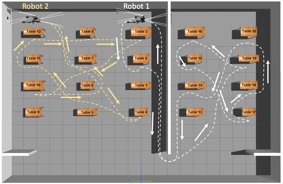
(a) The simulated environment for disinfection application with 20 tasks and 2 robots.

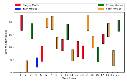
(b) The distribution of time-windows for 20-2-0.4 instance.

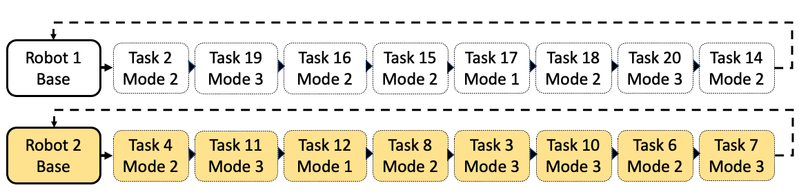
(c) The route sequences for instance with 20 tasks, 2 robots, mission time of 0.4 hours and with $\lambda=0.8$.

Figure 2: (a) The routes of two robots executing various tasks in the simulated environment. The route of the first robot is highlighted in white and for the second robot yellow is used. (b) The plot shows the distribution of time windows in which the respective task must be completed. The mission time for this instance is 24 minutes. The number of task execution modes for each task is depicted by the color. (c) The route sequence taken by each robot. For $\lambda=0.8$, maximization of the number of tasks completed has more emphasis than the quality of disinfection. As a result, most of the tasks are done in higher modes.

In this section, we evaluate the proposed problem. The utility of M³RS in comparison to routing and scheduling in fixed disinfection mode is demonstrated on the synthetically generated dataset. Next, we showcase the application of the proposed formulation in a case-study of simulated and real-world surface disinfection missions. Finally, we perform sensitivity analysis on M³RS by varying the fleet size of the robots and relaxing the starting times for the tasks.

IV-A Evaluation on Synthetic Dataset

In this experiment, the performance of M³RS is compared with the routing and scheduling with fixed (RS-F) disinfection mode. The mixed integer programming formulation of RS-F is the same as the vehicle routing problem with time windows [28]. For M³RS, the mixed integer programming formulation results solved using branch and cut and column generation (CG) are reported.

Table II: Results for synthetic dataset. The M³RS formulation provides more choices for the user to trade-off between DQ and SR. Further, the MSI metric for M³RS is better than the fixed mode, indicating better performance for joint metrics.

Instance Type	Algorithm	$\lambda$	SR	DQ	MSI	CT (s)	Opt.
20-2-0.86	M3RS	0.5	0.75	0.86	0.70	4.2	O
		0.8	0.80	0.73	0.69	4.6	O
		0.1	0.70	0.94	0.68	5.5	O
2-8	M3RS (CG)	0.5	0.80	0.76	0.70	22.2	F
		0.8	0.85	0.63	0.68	24.5	F
		0.1	0.75	0.88	0.70	25.3	F
2-8	RS-F (Max)	NA	0.65	1.0	0.65	4.5	O
	RS-F (Min)	NA	0.85	0.48	0.63	6.8	O
20-2-0.46	M3RS	0.5	0.65	0.6	0.52	361.1	O
		0.8	0.7	0.45	0.57	233.6	O
		0.1	0.50	0.94	0.50	114.9	O
2-8	M3RS (CG)	0.5	0.65	0.63	0.53	101.1	F
		0.8	0.70	0.48	0.52	100.6	F
		0.1	0.55	0.87	0.51	101.2	F
2-8	RS-F (Max)	NA	0.45	1.0	0.48	6.0	O
	RS-F (Min)	NA	0.75	0.30	0.45	128.9	O
40-3-1.15	M3RS	0.5	0.90	0.63	0.73	200	F
		0.8	0.95	0.52	0.72	1200.0	F
		0.1	0.77	0.80	0.69	1200.0	F
2-8	M3RS (CG)	0.5	0.85	0.64	0.70	142.1	F
		0.8	0.85	0.58	0.67	200.7	F
		0.1	0.75	0.83	0.68	169.2	F
2-8	RS-F (Max)	NA	0.55	1.0	0.55	117.4	O
	RS-F (Min)	NA	0.87	0.37	0.60	1200.0	F
40-3-0.55	M3RS	0.5	0.52	0.71	0.45	1200.0	F
		0.8	0.60	0.45	0.43	1200.0	F
		0.1	0.45	0.88	0.42	1200.0	F
2-8	M3RS(CG)	0.5	0.57	0.47	0.43	95.6	F
		0.8	0.60	0.43	0.43	148.2	F
		0.1	0.42	0.93	0.41	105.3	F
2-8	RS-F (Max)	NA	0.40	1.0	0.40	1200.0	F
	RS-F (Min)	NA	0.55	0.36	0.42	1200.0	F
80-3-2.13	M3RS	0.5	0.80	0.78	0.71	1200.1	F
		0.8	0.82	0.67	0.68	1200.1	F
		0.1	0.75	0.89	0.71	1200.1	F
2-8	M3RS(CG)	0.5	0.62	0.79	0.56	402.2	F
		0.8	0.40	0.75	0.35	517.1	F
		0.1	0.61	0.85	0.56	376.8	F
2-8	RS-F (Max)	NA	0.61	1.0	0.61	1200.1	F
	RS-F (Min)	NA	0.53	0.40	0.46	1200.1	F
80-4-0.77	M3RS	0.5	0.38	0.78	0.35	1200.1	F
		0.8	0.45	0.67	0.37	1200.1	F
		0.1	0.35	0.89	0.33	1200.1	F
2-8	M3RS (CG)	0.5	0.46	0.70	0.39	217.7	F
		0.8	0.52	0.43	0.37	218.5	F
		0.1	0.40	0.90	0.38	214.0	F
2-8	RS-F (Max)	NA	0.20	1.0	0.20	1200.1	F
	RS-F (Min)	NA	0.16	0.38	0.11	1200.2	F
Opt = Optimality of solutions, O = Optimal, F= Feasible

Experiment Setup: A synthetic dataset compares the M³RS and RS-F. For this experiment, we consider two variants of RS-F called max and min. The max variant uses only the mode corresponding to the highest disinfection dosage. The min variant only uses the mode with the lowest disinfection dosage. The M³RS creates schedules while considering all the disinfection modes. The objective in M³RS depends on the quality factor ($\lambda$), which dictates the user preference of task completion vs disinfection quality. We report results of M³RS for $\lambda=0.8,\,0.5,\,0.1$. Both cases of RS-F, i.e., max and min, are implemented on CPLEX [29] with the maximum compute time fixed to $20$ minutes. The restricted master problem and sub-problem for CG are implemented on CPLEX [29]. All the experiments are carried out on a machine equipped with an Intel i5 dual-core processor with 8 GB RAM. The maximum compute time for column generation is $10$ minutes. We use the following metrics for comparison:

$$SR\,=\,\frac{\sum_{k\in\mathcal{A}}\sum_{i\in\mathcal{T}}\sum_{j\in\mathcal{T}}x^{k}_{i\scriptsize{\xrightarrow{}}j}}{|\mathcal{T}|}$$ (22)

$$DQ\,=\,\frac{\sum_{k\in\mathcal{A}}\sum_{i\in\mathcal{T}}\sum_{m\in\mathcal{M}_{i}}y^{k}_{i,m}}{\sum_{k\in\mathcal{A}}\sum_{i\in\mathcal{T}}\sum_{j\in\mathcal{T}}x^{k}_{i\scriptsize{\xrightarrow{}}j}}$$ (23)

$$MSI\,=\,\frac{\sum_{k\in\mathcal{A}}\sum_{i\in\mathcal{T}}\sum_{j\in\mathcal{T}}\sum_{m\in\mathcal{M}_{i}}x^{k}_{i\scriptsize{\xrightarrow{}}j}+p_{i,m}\cdot y^{k}_{i,m}}{|\mathcal{T}|\cdot(1+p^{max})}$$ (24)

The success rate ($SR$) indicates the number of tasks completed successfully. The dosage quality ($DQ$) indicates the disinfection quality of completed tasks. The mission success index ($MSI$) is a combined metric that is the ratio of the sum of the number of tasks completed and the disinfection quality with respect to the total number of tasks and associated reward for maximum disinfection quality. Further, we report computation times (CT) and whether a solution is optimal or feasible, indicated by letters O and F, respectively.

Data Generation: The dataset consists of multiple instances with a different number of tasks and their time windows. For each instance, we assume that the robotic base and manipulator arm operate at a constant speed. Further, we assume that each disinfection task is a desk. The location for each task is assumed to be spread in a $30m\times 30m$ area. This emulates a large hospital floor where the tasks are distributed across various locations. In the experiments, we consider four disinfection modes corresponding to disinfection levels of $99.9999\%$, $99.99\%$, $99\%$, and $90\%$. Each task $i$ is randomly assigned a mode set ($\mathcal{M}_{i}$) with $1$ to $4$ disinfection modes. For each mode, a disinfection dosage, disinfection times, and energy consumption is specified. A mission time horizon is defined for each instance. The time window for all tasks is spread across the mission time horizon. The distances between all the locations are calculated using Euclidean distance. The travel times are calculated using a fixed velocity of the robot base. Finally, the energy consumption for travel and disinfection dosage is determined using a simple battery model. We generate six test instances based on combinations of the number of tasks, the number of robots, and mission times. Each test instance name consists of three numbers. The first one represents the number of tasks, the second is the number of robots, and the third indicates the mission time in hours. For example, a 20-2-0.86 instance is a mission with 20 tasks, 2 robots, and a mission time of 0.86 hours. Different test instances used are listed in Table II. We provide test instances with different mission times. This is done to simulate a variety of available time slots for disinfection operations in institutes with time constraints like hospitals.

Discussion: The results for M³RS and fixed mode variants on different instances are given in Table. II. Since the max variant defaults to the highest disinfection, it had the highest DQ index for all instances. But, it has the lowest SR index for all cases. This is because higher modes of disinfection are time-intensive due to which only a limited number of tasks are addressed. On the contrary, the min variant offers the highest SR index as the disinfection time per task is small. However, the DQ index is low for the min variant. The solutions with M³RS provide competitive SR and DQ compared to the fixed variants. Furthermore, these solutions have the highest MSI score. This indicates that the mode selection framework offers better flexibility and, hence, better solutions. The users can specify $\lambda$ based on their requirements. For example, when disinfection quality is a priority a smaller value of $\lambda$ should be used and a higher value is preferred when task completion is the requirement. It is seen from the results that for both M³RS and RS-F variants, the computation time increases significantly with an increase in the problem size. The column generation method can closely approximate the results of exact formulation with a relatively smaller compute time. Hence, column generation can be used to solve applications with many tasks and many robots.

IV-B Simulated and Hardware Case Study

In the simulation and hardware case study, we showcase the application of M³RS for disinfection missions addressed by a team of G-robots [12]. Multiple disinfection mission instances are generated for a simulated environment. Each disinfection mission is characterized by mission time, time windows for each task, and number of robots used in the mission. The simulated environment consists of $20$ tables as disinfection surfaces spread across two rooms. The number of robots used ranges from 2-5 robots. Ideally, the mission times are inversely proportional to the number of robots used in the mission because fewer robots would require more time to do the same number of tasks. A sample distribution of time windows for each task in one of the missions is depicted in Fig. 2 (b). The entire simulated experiment is conducted in ROS [30] and Gazebo environment [31]. For the hardware case study, we use two G-robots for a disinfection mission consisting of six tables. Each table can be disinfected in three disinfection modes, i.e. $99.99\%$, $99\%$, and $90\%$. The entire disinfection mission must be completed in $17$ minutes. The time distribution for different tasks is given in Fig. 3(a). For both cases, M³RS is solved for two preferences: $\lambda\,=0.8$ and $0.1$ for each mission. The optimization model is solved in CPLEX. The metrics reported include SR, DQ, MSI, optimality of the solutions, and average lateness of the robot in task completion.

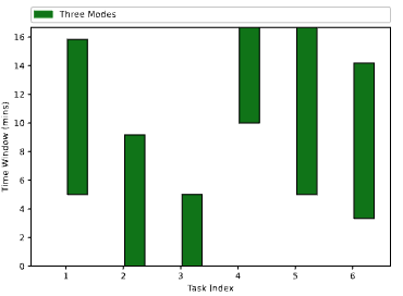
(a) The distribution of time-windows for hardware experiment with 6 tasks, 2 robots and mission time 0f 0.28 hours.

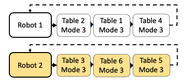
(b) The route sequence for $\lambda=0.9$

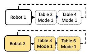
(c) The route sequence for $\lambda=0.1$

Figure 3: (a) The plot shows the distribution of time windows in which the respective tables must be disinfected. (b) & (c) The route sequence taken by each robot for $\lambda=0.9$ and $0.1$. For $\lambda=0.9$, the emphasis is on disinfecting all the tables at higher disinfection modes. Whereas, for $\lambda=0.1$, the emphasis is on ensuring high-quality disinfection rather than disinfecting all tables.

Discussion: The results for simulated and hardware case studies are given in Table III. The example of generated route sequences are shown in Fig. 2 (b)-(c) for simulated cases and in Fig. 3 (b)-(c) for the hardware instance. It can be seen that a decent success rate is achieved in all missions. This indicates that for smaller mission times, a larger robotic fleet would be necessary to cover different tasks. The trade-off between SR and DQ is more evident in the two robot missions. In other missions, each task has a smaller time window, which means many of the tasks cannot be performed in higher disinfection modes, see Fig. 2. Finally, there are some minor delays observed in terms of task completion times for simulation and hardware implementation. These delays are caused by slightly longer path planning times. Such delays can be accounted for by introducing chance constraints to model stochasticity in the system.

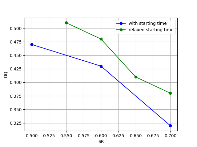
(a) The Pareto front for relaxed starting time and with time window constraints.

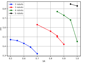
(b) The Pareto front with varying size of the robotic fleet.

Figure 4: (a) The plot demonstrates the improvement in performance metrics by relaxing the starting time. (b) Increasing the number of robots in the fleet improves the performance metrics for a given mission.

Table III: Results for simulated experiments. The simulated and hardware instances showcase the trade-offs in SR and DQ metrics for different user preferences.

Instance Type	$\lambda$	SR	DQ	MSI	Optimality	Avg. Lateness (s)
20-2-0.40	0.80	0.80	0.57	0.63	O	1.9
	0.10	0.70	0.71	0.60	O	6.2
20-3-0.21	0.80	0.80	0.51	0.60	F	30.1
	0.10	0.75	0.56	0.58	F	1.4
20-4-0.20	0.80	0.95	0.55	0.74	F	33.6
	0.10	0.90	0.60	0.72	F	19.1
20-5-0.16	0.80	0.80	0.57	0.68	F	29.4
	0.10	0.75	0.62	0.68	F	33.7
6-2-0.28*	0.90	1.00	0.40	0.70	O	27.0
	0.10	0.67	1.00	0.65	O	32.0
* = Results for hardware experiments.

IV-C Sensitivity Analysis

We analyze the variation in solutions of M³RS for two cases. In the first case, the starting times for all the tasks in the mission are relaxed. This case is relevant for applications that require a task to be finished by a deadline and are agnostic to the starting time of the task. The second case studies the impact of using more robots for a given mission. We use the 20-2-0.46 instance from the synthetic dataset to benchmark both cases. The preferences used for M³RS are in the range of $\lambda\,=0-1$. Note that all the cases are implemented on same set of values of $\lambda$. The optimization model is solved in CPLEX. The results are graphically visualized as the Pareto front between SR and DQ in Fig. 4.

Discussion: Relaxing the starting time significantly improves the solution quality in terms of both SR and DQ. This is evident from the Pareto front shown in Fig. 4(a). This improvement is expected, as relaxing the starting times enables the fleet to address more tasks with possibly better task quality. Hence, a relaxing starting time for tasks would be a better choice when task completion is only concerned with the associated deadlines. As seen in Fig. 4(b), increasing the fleet size significantly improves SR and DQ metrics. Using more robots is particularly useful for shorter mission times with many tasks. However, using more robots will make the overall operation costlier.

V Conclusions and Future work

In this work, we proposed M³RS, a novel multi-objective formulation that routes and schedules a team of agents to accomplish various tasks in a mission. The agents can perform the task in one of many available modes. Each mode has distinct task quality, resource consumption, and service times. We first propose a mixed-integer linear programming model for M³RS. Then, a column generation approach is presented to tackle larger instances with a faster computation time. We showcase the utility of M³RS in multi-robot disinfection applications. The experiments suggest that our solution for M³RS provides more flexibility to users to select solutions based on desired preferences. The current approach is limited as it assumes a deterministic environment, unlike real-world scenarios. Generating the entire Pareto front is computationally expensive, particularly for larger instances. Our future work will extend M³RS to incorporate elements like stochastic travel times and dynamic arrival of jobs. Further, we will investigate using deep reinforcement learning as a faster alternative to generate a Pareto solution set for M³RS.

References

- [1] H. Shen, L. Pan, and J. Qian, “Research on large-scale additive manufacturing based on multi-robot collaboration technology,” Additive Manufacturing, vol. 30, p. 100906, 2019.
- [2] P. Ghassemi and S. Chowdhury, “Multi-robot task allocation in disaster response: Addressing dynamic tasks with deadlines and robots with range and payload constraints,” RAS, vol. 147, p. 103905, 2022.
- [3] F. Leofante, E. Ábrahám, T. Niemueller, G. Lakemeyer, and A. Tacchella, “Integrated synthesis and execution of optimal plans for multi-robot systems in logistics,” ISF, vol. 21, pp. 87–107, 2019.
- [4] B. P. Gerkey and M. J. Matarić, “A formal analysis and taxonomy of task allocation in multi-robot systems,” IJRR, vol. 23, no. 9, pp. 939–954, 2004.
- [5] G. A. Korsah, A. Stentz, and M. B. Dias, “A comprehensive taxonomy for multi-robot task allocation,” IJRR, vol. 32, no. 12, pp. 1495–1512, 2013.
- [6] E. F. Flushing, L. M. Gambardella, and G. A. Di Caro, “Simultaneous task allocation, data routing, and transmission scheduling in mobile multi-robot teams,” in 2017 IROS. IEEE, 2017, pp. 1861–1868.
- [7] S. Hayat, E. Yanmaz, C. Bettstetter, and T. X. Brown, “Multi-objective drone path planning for search and rescue with quality-of-service requirements,” Autonomous Robots, vol. 44, no. 7, pp. 1183–1198, 2020.
- [8] M. Lahijanian, M. Svorenova, A. A. Morye, B. Yeomans, D. Rao, I. Posner, P. Newman, H. Kress-Gazit, and M. Kwiatkowska, “Resource-performance tradeoff analysis for mobile robots,” IEEE RAL, vol. 3, no. 3, pp. 1840–1847, 2018.
- [9] L.-L. Dai, Q.-K. Pan, Z.-H. Miao, P. N. Suganthan, and K.-Z. Gao, “Multi-objective multi-picking-robot task allocation: Mathematical model and discrete artificial bee colony algorithm,” IEEE Transactions on Intelligent Transportation Systems, 2023.
- [10] X. Chen, S. He, Y. Zhang, L. C. Tong, P. Shang, and X. Zhou, “Yard crane and agv scheduling in automated container terminal: A multi-robot task allocation framework,” Transportation Research Part C: Emerging Technologies, vol. 114, pp. 241–271, 2020.
- [11] M. Hojda, “Task allocation in robot systems with multi-modal capabilities,” IFAC-PapersOnLine, vol. 48, no. 3, pp. 2109–2114, 2015.
- [12] I. Mehta, H.-Y. Hsueh, N. Kourtzanidis, M. Brylka, and S. Saeedi, “Far-uvc disinfection with robotic mobile manipulator,” in 2022 International Symposium on Medical Robotics (ISMR). IEEE, 2022, pp. 1–8.
- [13] N. Wilde and J. Alonso-Mora, “Statistically distinct plans for multi-objective task assignment,” arXiv preprint arXiv:2312.07292, 2023.
- [14] J. G. Martin, J. R. D. Frejo, R. A. García, and E. F. Camacho, “Multi-robot task allocation problem with multiple nonlinear criteria using branch and bound and genetic algorithms,” Intelligent Service Robotics, vol. 14, no. 5, pp. 707–727, 2021.
- [15] C. Wei, Z. Ji, and B. Cai, “Particle swarm optimization for cooperative multi-robot task allocation: a multi-objective approach,” IEEE RAL, vol. 5, no. 2, pp. 2530–2537, 2020.
- [16] M. Calzavara, M. Faccio, and I. Granata, “Multi-objective task allocation for collaborative robot systems with an industry 5.0 human-centered perspective,” The IJAMT, vol. 128, no. 1-2, pp. 297–314, 2023.
- [17] Y. Y. Liau and K. Ryu, “Genetic algorithm-based task allocation in multiple modes of human–robot collaboration systems with two cobots,” The IJAMT, vol. 119, no. 11-12, pp. 7291–7309, 2022.
- [18] C. Ferreira, G. Figueira, and P. Amorim, “Scheduling human-robot teams in collaborative working cells,” IJPE, vol. 235, p. 108094, 2021.
- [19] S. Hartmann and D. Briskorn, “An updated survey of variants and extensions of the resource-constrained project scheduling problem,” EJOR, vol. 297, no. 1, pp. 1–14, 2022.
- [20] J. Alcaraz, C. Maroto, and R. Ruiz, “Solving the multi-mode resource-constrained project scheduling problem with genetic algorithms,” JORS, vol. 54, no. 6, pp. 614–626, 2003.
- [21] M. Caramia and S. Giordani, “A fast metaheuristic for scheduling independent tasks with multiple modes,” Computers & Industrial Engineering, vol. 58, no. 1, pp. 64–69, 2010.
- [22] C. Tilk, K. Olkis, and S. Irnich, “The last-mile vehicle routing problem with delivery options,” Or Spectrum, vol. 43, no. 4, pp. 877–904, 2021.
- [23] M. Seyfi, M. Alinaghian, E. Ghorbani, B. Çatay, and M. S. Sabbagh, “Multi-mode hybrid electric vehicle routing problem,” Transportation Research Part E: Logistics and Transportation Review, vol. 166, p. 102882, 2022.
- [24] I. Kara, G. Laporte, and T. Bektas, “A note on the lifted miller–tucker–zemlin subtour elimination constraints for the capacitated vehicle routing problem,” EJOR, vol. 158, no. 3, pp. 793–795, 2004.
- [25] I. Mehta, H.-Y. Hsueh, S. Taghipour, W. Li, and S. Saeedi, “Uv disinfection robots: a review,” RAS, vol. 161, p. 104332, 2023.
- [26] J. Desrosiers and M. E. Lübbecke, “A primer in column generation,” in Column generation. Springer, 2005, pp. 1–32.
- [27] M. E. Lübbecke and J. Desrosiers, “Selected topics in column generation,” Operations research, vol. 53, no. 6, pp. 1007–1023, 2005.
- [28] B. Kallehauge, J. Larsen, O. B. Madsen, and M. M. Solomon, Vehicle routing problem with time windows. Springer, 2005.
- [29] P. Laborie, J. Rogerie, P. Shaw, and P. Vilím, “Ibm ilog cp optimizer for scheduling: 20+ years of scheduling with constraints at ibm/ilog,” Constraints, vol. 23, pp. 210–250, 2018.
- [30] M. Quigley, K. Conley, B. Gerkey, J. Faust, T. Foote, J. Leibs, R. Wheeler, and A. Y. Ng, “ROS: an open-source Robot Operating System,” in ICRA workshop on open source software, vol. 3, no. 3.2. Kobe, Japan, 2009, p. 5.
- [31] N. Koenig and J. Hsu, “The many faces of simulation: Use cases for a general purpose simulator,” in Proc. of the ICRA, vol. 13, 2013, pp. 10–11.