The APO-K2 Catalog. II. Accurate Stellar Ages for Red Giant Branch Stars Across the Milky Way

Abstract

We present stellar age determinations for 4,661 red giant branch (RGB) stars in the APO-K2 Catalog, derived using mass estimates from K2 asteroseismology from the K2 Galactic Archaeology Program and elemental abundances from the Apache Point Galactic Evolution Experiment (APOGEE) survey. Our sample includes 17 of the 19 fields observed by K2, making it one of the most comprehensive catalogs of accurate stellar ages across the Galaxy in terms of the wide range of populations spanned by its stars, enabling rigorous tests of Galactic chemical evolution models. Taking into account the selection functions of the K2 sample, the data appear to support the age-chemistry morphology of stellar populations predicted by both inside-out and late-burst scenarios. We also investigate trends in age versus stellar chemistry and Galactic position, which are consistent with previous findings. Comparisons against APOKASC-3 asteroseismic ages show agreement to within $\sim$3%. We also discuss offsets between our ages and spectroscopic ages. Finally, we note that ignoring the effects of $\alpha$-enhancement on stellar opacity (either directly or with the Salaris metallicity correction) results in an $\sim$10% offset in age estimates for the most $\alpha$-enhanced stars, which is an important consideration for continued tests of Galactic models with this and other asteroseismic age samples.

1 Introduction

The complex formation history of the Milky Way (MW) is both important to understand and difficult to decode. Stellar ages are a crucial clue, complementing studies of stellar positions, dynamics, and composition. However, due to the fact that the observed properties of stars are mostly insensitive to age, precise and accurate ages of stars are difficult to infer.

With the rise of ensemble asteroseismology over the last two decades—thanks to large-scale, space-based, time-domain surveys such as CoRoT (Baglin, 2003), Kepler (Borucki et al., 2010), K2 (Howell et al., 2014), and TESS (Ricker et al., 2015)—it is possible to measure solar-like oscillation patterns in many stars. These oscillations are due to near-surface turbulent convection motions that generate sound waves. These sound waves, when at distinct resonant frequencies in the stellar interior, create standing waves that form a frequency pattern of overtone modes of differing spherical degree and radial order. The characteristic spacing between these frequencies, known as the large frequency-spacing ($\Delta\nu$), is related to the mean density of the star (Tassoul, 1980; Kjeldsen & Bedding, 1995). The frequency of maximum acoustic power ($\nu_{\rm max}$) is related to the acoustic cutoff frequency, and therefore the density scale height and surface gravity of the star (Brown et al., 1991; Kjeldsen & Bedding, 1995). These global parameters allow us to derive the masses of the stars through well-understood scaling relations as long as these two parameters and the stars’ effective surface temperatures ($T_{\mathrm{eff}}$) are known. These mass measurements, along with composition information, allow model-based age determinations.

Analyses from asteroseismic data have been significantly furthered due to support from similarly large, ground-based, spectroscopic surveys such as the Apache Point Galactic Evolution Experiment (APOGEE; Majewski et al. 2017), The Large Sky Area Multi-Object Fibre Spectroscopic Telescope (LAMOST) survey (Cui et al., 2012), and the GALactic Archaeology with HERMES (GALAH) survey (De Silva et al., 2015). These surveys, in select cases, have intentionally large overlaps with targets from space-based asteroseismic missions. The resulting ages due to the combination of spectroscopic compositions and temperatures with asteroseismic masses have allowed significant work in Galactic archaeology, revealing the Galaxy’s evolution history by linking stellar chemistry and age at Galaxy-wide scales (e.g., Anders et al. 2017, Silva Aguirre et al. 2018, Rendle et al. 2019, Miglio et al. 2021, Willett et al. 2023, Imig et al. 2023, Stokholm et al. 2023).

One avenue through which the formation of the MW can be examined with stellar compositions is by comparing populations of $\alpha$-rich versus $\alpha$-poor stars (as discussed by, e.g., Aller & Greenstein 1960 and Wallerstein 1962). These stars are rich (or poor) in $\alpha$-capture elements (e.g., Mg, O) compared to the Sun. The mix of heavy elements in stars is not universal; instead, it arises from distinct sources contributing on different timescales. As a result, regions with rapid star formation will have a different mix of elements versus regions with more gradual, or episodic, star formation. $\alpha$ elements are primarily produced in core-collapse supernova (SNe II), which—owing to their massive, short-lived progenitors—have rates that closely track the Galaxy’s (at least the local) star formation history (SFH). SNe Ia, a significant source of iron-peak elements, only enrich the interstellar medium at later times due a combination of the longer lifetime of intermediate-mass SNe Ia progenitors and delay time distributions from Chandrasekhar mass overflow (Timmes et al., 1995; Kobayashi et al., 1998; Ruiter et al., 2009). In models of Galactic star formation, as the Galaxy evolves and the rate of SNe Ia increases, the predicted ${\rm[\alpha/Fe]}$ of new stars simultaneously decreases as the Fe-peak elements become more abundant. Eventually, an equilibrium ratio is reached (e.g., Weinberg et al. 2017).

Regardless, this expected trend is not observed in the solar neighbourhood (Prochaska et al., 2000; Bensby et al., 2003); rather, stars with $-1<{\rm[Fe/H]}<0$ present a discontinuous range of [$\alpha$/Fe] values. This has become known as the $\alpha$ bi-modality, due to its bi-modal distribution and a distinct ridge-line in [$\alpha$/Fe] vs. [Fe/H] space. Investigations have led to further discoveries related to the $\alpha$ bi-modality, such as the relationship between $\alpha$-richness and the geometrically and kinematically defined thin and thick disks (e.g., Gilmore & Reid, 1983; Bovy et al., 2012; Hayden et al., 2015).

The literature presents several Galactic chemical evolution models that attempt to explain the observed spatial, chemical, and age trends associated with the $\alpha$ bi-modality. One class of models explains the $\alpha$ bi-modality with an initial, rapid star formation episode that forms the $\alpha$-rich population, with a subsequent lull in star formation that is pierced by an infall of pristine gas. This resets the metallicity of the disk, and quiescent formation proceeds to form the $\alpha$-poor population (“two-infall”; e.g., Chiappini et al. 1997; Spitoni et al. 2019). Another class of models describes two separate star formation episodes for the $\alpha$-rich disk and the $\alpha$-poor disk: the inner disk forms an $\alpha$-rich population at early times, followed by a smooth transition to an $\alpha$-poor population, with the inner part of the $\alpha$-poor population having higher metallicity than the outer part due to forming from the gas enriched by the inner disk (Haywood et al., 2013; Ciucă et al., 2021). An alternate scenario described by Schönrich & Binney (2009) and expanded by Sharma et al. (2021b) envisions a disk whereby stars occupying a wide range in chemical space are born simultaneously, though at higher rates in the inner disk than the outer disk. This causes $\alpha$-poor stars born in the slow chemical enrichment environment of the outer disk to have low metallicities that are otherwise associated with $\alpha$-rich stars. Radial migration (e.g., Sellwood & Binney, 2002) then brings populations of different chemistry into the solar neighborhood, causing the observed $\alpha$ bi-modality. A more recent model (Clarke et al., 2019) predicts overlap in ages between $\alpha$-rich and $\alpha$-poor populations thanks to a clumpy star formation scenario, where star formation proceeds at different rates simultaneously throughout the disk in small clumps.

Although models have been shown to reproduce observed abundance and spatial trends, there has been little direct comparison between these model predictions and observed age-abundance patterns beyond generic predictions that the $\alpha$-rich population should be generally older than the $\alpha$-poor population. The consideration of the age trends in [Fe/H]-$\alpha$ space is therefore a potentially crucial test of these models, which we investigate here using comparisons between asteroseismic ages and the Galactic chemical evolution model of Johnson et al. (2021).

In this paper, we expand on the work presented by Warfield et al. (2021), where asteroseismic-based ages were derived for 735 RGB stars across three K2 campaigns. Here, we present accurate age measurements for 4,661 RGB stars from the APO-K2 Catalog (Schonhut-Stasik et al. 2024, hereafter JSS24), a cross-match between the asteroseismic K2 Galactic Archaeology Program (K2 GAP) catalog (Stello et al., 2015, 2017) and APOGEE DR17. Thanks to the observing strategy forced upon the K2 mission, this catalog provides asteroseismic and spectroscopic parameters along 17 lines of sight in the MW, making it one of the most comprehensive asteroseismic-spectroscopic surveys of the diverse populations of our Galaxy to date.

In §2, we discuss our data selection, showcasing the spectroscopic data in §2.1, the asteroseismic data in §2.2, and the selection function in §2.3. In §2.4, we discuss the cuts we have made to the APO-K2 data set. In §3, we detail our methods (§3.1), our comparison with the APOKASC-3 methodology (§3.2), and the effects of $\alpha$-abundance on age determination (§3.3). We compare our ages with spectroscopic ages from AstroNN (Mackereth et al., 2019) in §3.4. We move on to analysing our population in §4, with a discussion of the K2 fields in §4.1, similarities between the Kepler field and the K2 fields in §4.2, stellar age and chemistry as a function of Galactic position in §4.3, and a comparison to modeled populations from Johnson et al. (2021) in §4.4. We conclude and discuss our results in-context in §5. In addition to the online journal, age data is publicly available for the APO-K2 catalog at https://github.com/jesstella/apo-k2 and https://github.com/jackwarfield/apo-k2.

2 Data

Our base data set is the APO-K2 Catalog (JSS24), a cross-match between data from the K2 Galactic Archaeology Program Data Release 3 (K2 GAP DR3; Zinn et al. 2022), the Apache Point Observatory Galactic Evolution Experiment Data Release 17 (APOGEE DR17; Majewski et al., 2017; Abdurro’uf et al., 2022), and Gaia DR3 (Gaia Collaboration et al., 2016, 2023). In addition to this summary of the data, we detail the entire data pipeline, from K2 light curves to ages, in Appendix A.

2.1 Spectroscopic Data

APOGEE DR17 is a part of the final data release of the Sloan Digital Sky Survey Phase IV (SDSS-IV; Blanton et al., 2017) and provides high-resolution near-infrared spectra (using twin, $R\sim 22{,}500$ $H$-band spectrographs; Wilson et al. 2019) for 657,000 unique targets (with targeting described by Beaton et al. 2021), encompassing observations dating back to the first edition of the APOGEE survey during SDSS Phase III in 2011. Spectra were collected using the 2.5-meter Sloan Foundation Telescope (Gunn et al., 2006) at the Apache Point Observatory in New Mexico, USA (APOGEE-North) from 2011-2020 and the 2.5-meter du Pont Telescope (Bowen & Vaughan, 1973) at Las Campanas Observatory in Chile (APOGEE-South) from 2017-2020.

In addition to providing the raw data, APOGEE spectra have been put through a reduction pipeline that, in the end, provides spectrally-derived and calibrated estimates for stellar parameters such as effective temperature ($T_{\rm eff}$), log surface gravity ($\log{g}$), and chemical abundances (including ${\rm[Fe/H]}$ and ${\rm[\alpha/M]}$). Nidever et al. (2015; with updates from Holtzman et al. 2018 and Jönsson et al. 2020) describe the schema for extracting the spectra and performing wavelength calibrations, flat-fielding, and measuring radial velocities.

2.2 Asteroseismic Data

K2 GAP (Stello et al., 2015) is the source for the asteroseismic data that we use in this work. The targeting for the program used simple color and magnitude cuts to select a sample of red giant solar-like oscillators, prioritizing bright and red targets. Dwarfs, which would not oscillate at low enough frequencies to be detected with K2 long-cadence data, were additionally selected against using a reduced proper motion selection cut. Details of the selection function can be found in Sharma et al. (2022). The result is a well-understood sample ideal for Galactic archaeology applications.

Zinn et al. (2022) derived values for the asteroseismic parameters $\nu_{\rm max}$ and $\Delta\nu$. These derived values for each star are made from the amalgamation of values from six independent pipelines, each based on an independent analysis of K2 light-curves, corrected for instrumental systematics (Luger et al., 2018). We have further corrected $\Delta\nu$ using the prescription from Sharma et al. 2016 in combination with APOGEE DR17 abundances (see JSS24, and/or Appendix A.3, for details). Stellar surface gravities ($g$, or $\log{g}$), masses, and radii are derived using asteroseismic scaling relations, which are calibrated to be on the Gaia DR2 radius scale (see Zinn et al. 2022 and/or Appendix A.3).

2.3 Selection Function

Because the targeting strategy used for selecting potential solar-like oscillators for K2 GAP is distinct from that used for targeting the same fields for APOGEE (which is described by Beaton et al. 2021), the composite age of a given stellar population is potentially vulnerable to bias. The selection function between these two targeting strategies has been worked out, in part, by JSS24 (see also Appendix A.5) as functions of magnitude, color, mass, radius, $\nu_{\rm max}$, and metallicity. Additionally, JSS24 presents a selection function for translating from K2 GAP’s stellar distribution to the true Galactic stellar populations of detectable asteroseismic giants as indicated by Galaxia (Sharma et al., 2011).

In the analysis of our results in §4.2, we present the composite ages of our sample’s populations both un-scaled as well as scaled to the selection function in mass and metallicity that exists between the APO-K2 sample and the Galaxia model; i.e., this selection function allows us to re-scale the APO-K2 age distributions to how they should approximately have appeared if the sample truly represented an unbiased sample of the Galaxy’s asteroseismically detectable red giant population. The wider implications of accounting for selection functions for population age-dating is discussed in that section.

2.4 Cuts to the APO-K2 data set

The APO-K2 Catalog provides asteroseismically-derived masses and spectroscopic measurements of metallicity ([Fe/H]) and $\alpha$-element abundances ([$\alpha$/M]) for 7,672 red giant branch (RGB) and red clump (RC) stars. Stellar evolutionary states are assigned using a spectroscopic classification that has been calibrated using stars from the APOKASC-3 sample (M. Pinsonneault et al. 2024, in preparation), for which evolutionary states have been determined asteroseismically (our process is described in War21 using APOKASC-2 data, with updated parameters using APOKASC-3 provided in §2.3 of JSS24 as well as Appendix A.5). In this work, we derive stellar ages from stellar evolutionary tracks, using mass as a fundamental proxy for age. Therefore, we only consider stars for our analysis that are classified as being on the RGB. Though it is known that stars lose mass transitioning between the RGB and RC, without a detailed prescription of this change ages derived from the masses of RC stars will tend to be systematically biased to older ages (e.g., as shown by Casagrande et al. 2016; we discuss this further in Appendix B). We also limit the sample to stars with masses between 0.6 and 2.6 M_⊙, [$\alpha$/M] values between 0.0 and 0.4 dex, and [Fe/H] values between -1.0 and 0.6 dex, which is the parameter space encompassed by our evolutionary tracks and for which asteroseismic scaling relations are well behaved.

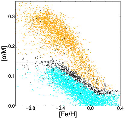
Figure 1: [$\alpha$/M] versus [Fe/H] for all stars in the K2 GAP sample. The black, dashed line represents our by-eye ridge-line to separate the $\alpha$-poor (cyan) from the $\alpha$-rich (orange) populations. The black unfilled markers represent stars that cannot be classified as either $\alpha$-poor or $\alpha$-rich with $>$95% confidence, due to the uncertainties in their chemical abundances.

In addition to our cuts, we have also defined two independent flags to categorize stars. The first is $\alpha$-rich versus $\alpha$-poor, which is made by drawing a ridge-line by-eye along the lower over-density of stars in the bi-modal [$\alpha$/M] vs. [Fe/H] distribution, with stars $\geq 2\sigma$ below the line being considered $\alpha$-poor (value of $0$ in the ALPHA_RICH_FLAG column) and above the line as $\alpha$-rich (ALPHA_RICH_FLAG = $1$). Stars falling within $2\sigma$ of this ridge-line are given neither classification (ALPHA_RICH_FLAG = $-1$). Our $\alpha$-rich versus $\alpha$-poor classifications are shown in Figure 1. The second classification is between the luminous and low-luminosity RGB (LL-RGB). Apropos asteroseismology, luminous giants are subject to measurement systematics due to the lower frequencies of their oscillations (versus their lower luminosity counterparts; Mosser et al. 2013, Pinsonneault et al. 2018, Zinn et al. 2019). War21 show that the larger uncertainties of the luminous giants are able to moderately diffuse the distribution of ages for a given population of stars beyond its intrinsic spread. We explore this again in §4, examining age distributions separately for stars with $\log{g}>2.5$, which we classify as low-luminosity.

3 Age Determination and Methodology Comparisons

3.1 Method

We have calculated underlying per-star age distributions in a manner identical to §3 of War21. Briefly, stellar evolutionary tracks generated with the Yale Rotating Evolution Code (YREC; Pinsonneault et al. 1989, with updates from van Saders & Pinsonneault 2012, and generated as described by Tayar et al. 2017) were used to create a regular grid (i.e., equally spaced along each axis), with axes for log(mass), [Fe/H], [$\alpha$/Fe], and log(age). Monte-Carlo sampling is used to draw sets of mass, [Fe/H], and [$\alpha$/M] values from each star’s distributions (which are assumed to be Gaussian), and the implied age for each draw is then estimated from the grid of evolutionary tracks via multi-dimensional four-point Lagrange interpolation. (See also Appendix A.6).

Table 1: The partial data table for the APO-K2 RGB sample, including our ages. The complete table is available in CSV format in the online journal, as well as with the APO-K2 catalog online at https://github.com/jesstella/apo-k2 and https://github.com/jackwarfield/apo-k2. The main identifier for each star is its ID in the Ecliptic Plane Input Catalog (EPIC). In addition to the columns shown here, our table contains Galactic longitude and latitudes; Galactocentric $R$ and $Z$ positions; the uncalibrated values for APOGEE $T_{\rm eff}$, $\log{g}$, [Fe/H], [$\alpha$/M], and [O/Fe], as well as the associated errors for all relevant columns. The $\alpha$-rich Flag column has a value of 1 for $\alpha$-rich stars, 0 for $\alpha$-poor stars, and -1 for unclassified stars. The S.F. Weight column is the weighting for that star given by the Galaxia selection function, and have been normalized so that the maximum weight is 100.

EPIC ID	APOGEE ID	Gaia EDR3 Source ID	RA	DEC	$T_{\rm eff}$	$\log(g)_{\rm APO}$	[Fe/H]	[$\alpha$/M]	[O/Fe]	$\alpha$-rich Flag	Mass	Radius	$\log(g)_{\rm seis}$	$\nu_{\rm max}$	$\Delta\nu$	Age	Modal Age	S.F. Weight
			(Deg.)	(Deg.)	(K)	($\log({\rm cm/s}^{2})$)	(dex)	(dex)	(dex)		(M⊙)	(R⊙)	($\log({\rm cm/s}^{2})$)	($\mu$Hz)	($\mu$Hz)	(Gyr)	(Gyr)
220648976	2M01161528$+$1009159	2580092098586391168	19.0637	10.1544	4947	3.13	-0.251	0.064	0.006		1.18	4.87	3.13	165.1	13.66	5.4	5.4	6.07
212123262	2M08302828$+$2228487	665901492034489600	127.6179	22.4802	4509	2.46	0.203	0.025	0.048		1.35	10.32	2.54	44.0	4.73	4.6	4.6	55.68
203757434	2M16095435$-$2502223	6049759992483427072	242.4765	-25.0395	4487	1.91	-0.663	0.312	0.371		0.60	12.47	2.03	13.5	2.38	45.7	30.0	0.51
212570575	2M13283736$-$1113561	3611427412665830784	202.1557	-11.2323	4797	3.06	-0.270	0.226	0.260		1.00	4.65	3.10	156.8	13.51	10.6	10.6	8.25
212458977	2M13271006$-$1336353	3609924895666745216	201.7919	-13.6098	4783	2.90	-0.378	0.265	0.357		0.97	5.46	2.95	110.1	10.44	11.3	11.3	5.94
206005182	2M22072683$-$1440432	6827450163146087168	331.8618	-14.6787	4702	3.19	0.289	0.060	0.077		1.16	8.86	2.61	50.4	5.52	8.5	8.0	70.08
212562020	2M13490785$-$1124552	3613482601761697024	207.2827	-11.4153	4874	3.09	-0.364	0.274	0.295		1.08	4.47	3.17	180.3	14.82	7.7	7.1	5.16
212396190	2M13564344$-$1500050	6301760184888854400	209.1810	-15.0014	4787	2.85	-0.439	0.290	0.324		0.92	5.64	2.90	98.2	9.70	13.1	12.7	4.70
205976299	2M22254038$-$1531593	2596147343468963840	336.4183	-15.5332	4989	3.14	-0.661	0.283	0.247		1.39	5.42	3.11	157.1	12.65	2.5	2.5	0.18
…	…	…	…	…	…	…	…	…	…		…	…	…	…	…	…	…	…

In War21, the median and $\pm 1\sigma$ percentiles of 500 log(age) values were reported for each star in the sample, and these values were used to construct the histograms and accompanying kernel-density estimations (KDEs) to discuss the overall characteristics of the populations. We repeat this process for our sample in this work, but have increased the number of runs from 500 to 5000 per star, made possible by optimizing the script from War21. In addition to median ages, we have also calculated ages defined by the mode of a KDE that we have fit over the 5000 log(age) values for each star individually. This is done with the intention of spotting potential biases on the median from extended tails in the age distributions to unphysically old ages ($\gtrapprox$14 Gyrs). However, we use the median age estimates for all of our analysis in this work. Our ages for the APO-K2 Catalog sample are available in Table 1 (as well as online at https://github.com/jesstella/apo-k2 and https://github.com/jackwarfield/apo-k2).

3.2 Ages in the Kepler Field and Comparison with an APOKASC-3 Methodology

Table 2: The partial data table for the re-calibrated APOKASC-2 RGB sample, including our ages. The complete table is available in CSV format in the online journal. The main identifier for each star is its ID in the Kepler Input Catalog (KIC), in the column KEPLER_ID. In addition to the columns shown here, our table contains Galactic longitude and latitudes; Galactocentric $R$ and $Z$ positions; the uncalibrated values for APOGEE $T_{\rm eff}$, $\log{g}$, [Fe/H] and [$\alpha$/M], as well as the associated errors for all relevant columns. The $\alpha$-rich Flag column has a value of 1 for $\alpha$-rich stars, 0 for $\alpha$-poor stars, and -1 for unclassified stars.

Kepler ID	APOGEE ID	Gaia EDR3 Source ID	RA	DEC	$T_{\rm eff}$	$\log(g)_{\rm APO}$	[Fe/H]	[$\alpha$/M]	$\alpha$-rich Flag	Mass	Radius	$\log(g)_{\rm seis}$	$\nu_{\rm max}$	$\Delta\nu$	Age	Modal Age
			(Deg.)	(Deg.)	(K)	($\log({\rm cm/s}^{2})$)	(dex)	(dex)		(M⊙)	(R⊙)	($\log({\rm cm/s}^{2})$)	($\mu$Hz)	($\mu$Hz)	(Gyr)	(Gyr)
8176543	2M19414369$+$4405382	2079615472445407744	295.4321	44.0939	4366	2.06		0.060	0	1.10	17.08	2.02	13.4	1.93	7.8	7.3
8277362	2M18440905$+$4417307	2117361186928151936	281.0377	44.2919	4507	2.40		0.260	1	0.96	10.64	2.37	29.4	3.65	12.6	12.7
2161831	2M19270967$+$3731187	2051785390040144640	291.7903	37.5219	4902	3.05		0.122	-1	1.06	4.94	3.08	145.0	12.41	7.6	7.4
6664533	2M18452413$+$4209269	2104693683403661952	281.3506	42.1575	4567	2.70		0.058	1	1.16	7.98	2.70	62.8	6.25	8.1	8.0
11723893	2M19473766$+$4949200	2087238180400724736	296.9069	49.8222	4651	2.80		0.035	0	1.15	6.83	2.83	84.1	7.88	8.0	7.9
10517437	2M18524613$+$4745349	2107664151504239104	283.1922	47.7597	3895	1.48		0.019	0	1.28	36.22	1.43	3.7	0.68	6.5	6.0
3441473	2M19232529$+$3833418	2052842158148906880	290.8554	38.5616	4643	2.57		0.295	1	0.99	7.84	2.65	55.3	5.90	11.0	10.9
6501676	2M18552344$+$4159111	2104874759224452096	283.8477	41.9864	4609	2.56		0.117	1	1.04	9.14	2.53	43.0	4.81	9.1	8.9
10272641	2M19250623$+$4718546	2129158263800815232	291.2760	47.3152	4859	2.86		0.063	0	1.29	6.95	2.87	89.8	8.17	3.9	3.9
…	…	…	…	…	…	…		…	…	…	…	…	…	…	…	…

Ages in the APOKASC-2 asteroseismic sample of stars in the Kepler field (as provided by Pin18, but also by, e.g., Silva Aguirre et al. 2018 for APOKASC-1), being one of the largest homogeneous sets of accurate age estimates to-date, have become a pillar for investigating the evolutionary history of the MW (e.g., Spitoni et al. 2019, Mackereth et al. 2019, Sharma et al. 2021a, Sharma et al. 2021b). Expecting that the upcoming update to this sample will play a similar role (APOKASC-3; M. Pinsonneault et al. 2024, in preparation), it is crucial to understand how the Kepler and K2 samples compare, both from methodological and astrophysical standpoints. Therefore, in addition to ages for the complete APO-K2 data set, we have calculated ages for the stars in the Kepler field, having recalculated the masses from Pin18 with new corrections to $\Delta\nu$ ($f_{\Delta\nu}$) calculated in the same manner as we have for APO-K2. As was done in Pin18, our masses for stars in the Kepler field have been calibrated from an open cluster contained in the data set, which carries a $2.1\%$ systematic uncertainty due to uncertainties in eclipsing binary mass measurements. Our data for the Kepler Field can be found in Table 2.

As noted in JSS24, K2 GAP DR3 $\nu_{\rm max}$ values were calibrated to a different scale than the APOKASC sample: the Gaia DR2-based astrometric scale (Gaia Collaboration et al., 2018), with a careful correction for parallax bias that took into account the different selection functions of RGB and RC stars (Schönrich & Aumer, 2017; Schönrich et al., 2019; Zinn et al., 2022). If we instead used parallaxes as corrected by the Gaia DR3 team without selection function corrections (Gaia Collaboration et al., 2018; Lindegren et al., 2021) to perform the calibration, this would result in an $\sim 4.5\%$ downward revision of the mass scale. We acknowledge potential variations in the Gaia calibration by noting a $2\%$ systematic uncertainty in the $\nu_{\rm max}$ calibration scale and $6\%$ in mass (Zinn et al., 2019) in the K2 data used in this work. Therefore, mass comparisons between K2 and Kepler could carry relative shifts with respect to each other up to a potential 6% in mass, or 20% in age. As we will see, it appears that the K2 and Kepler ages agree much better than this conservative estimate. We also note that whatever offsets there might be in the native K2 and Kepler $\nu_{\rm max}$ scales (e.g., due to differences in the time baselines of the datasets; Sharma et al. 2019; Zinn et al. 2022), are removed by this Gaia calibration.

War21 observed an offset of up to 2 Gyr between K2 stellar ages and those reported by Pin18. The authors postulated that this could have potentially been due to the lack of $\alpha$-enhanced interior opacities in the models used by Pin18, instead relying on the metallicity correction from Salaris et al. (1993); we explore this hypothesis more fully in the following subsection (§3.3).

One of the APOKASC-3 age determination methods will use mass (with no assumption for RGB mass-loss), $\log{g}$, [Fe/H], and [$\alpha$/M] as look-up parameters in a YREC stellar model grid (also from Tayar et al. 2017). For the sake of comparison, we have generated ages also using this APOKASC-3 methodology for all of the RGB stars in the APO-K2 sample. As our methodologies rely on the same axes within a common set of tracks, but utilize slightly different look-up procedures, this comparison should provide a valuable sense of our method’s systematic uncertainty.

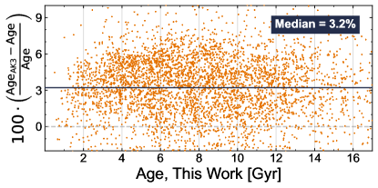
Figure 2: A comparison between the asteroseismic age determination method described in this work (and Warfield et al. 2021) and a method to be used for the APOKASC-3 catalog (M. Pinsonneault et al. 2024, in preparation). The x-axis is ages from this work, in Gyr, and the y-axis is the percent-offset of the ages found using the APOKASC-3 methodology. The gray, dashed line represents the one-to-one line and the blue, solid line tracks the measured median offset between the two ages.

The comparison between these ages is shown in Figure 2. In general, we see sufficient agreement between these ages, only with the APOKASC-3 methodology producing ages that are a median of 3.2% older than ours, and consistently $\lesssim$6% older than ours. Though not totally negligible on a star-by-star basis, this systematic offset is much smaller than the random uncertainties of our measurements.

One possible explanation for this zero-point offset is that it is due to how $\log{g}$ is taken into account by our different methods. In this work, we take the amount of time that a star spends on the main sequence (the main-sequence lifetime, or MSLT) as the age of a star. The time for a star to move up the RGB and onto the asymmetric giant branch is $\lesssim 10\%$ of its MSLT, and how far along on the RGB a star is will be associated with its $\log{g}$. Therefore, because this age-dating method from APOKASC-3 takes $\log{g}$ into account directly as a lookup parameter, it is possible to expect an average offset in ages at this level. Overall, this reminds us that age estimates from evolutionary tracks can be noticeably sensitive to methodology, even when working with the same sets of observational and theoretical data. This is especially relevant when taking into account that RGB ages derived from different stellar evolution codes also differ at the 2-5% level, even for similar physical inputs (Silva Aguirre et al., 2020).

3.3 Effects of Alpha-Abundance on Age Determination

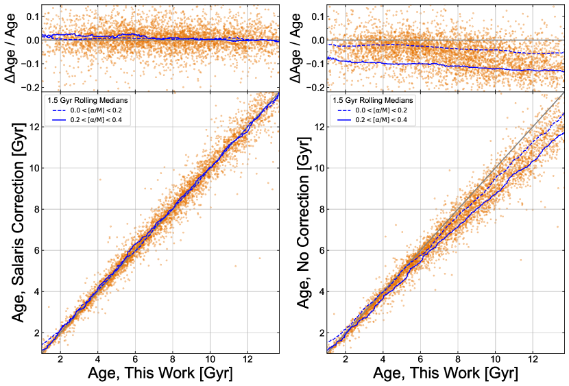
Figure 3: The left column of panels compares the ages for stars given in this work to the ages that would be obtained if interior opacity variations due to non-solar [$\alpha$/M] are not considered in the underlying evolutionary tracks, but rather each star’s metallicity is corrected using the formula from Salaris et al. (1993). The right column has the same x-axis, but the y-axis shows the ages inferred if the metallicities of stars are given no correction. The bottom panels compare these ages one-to-one, and the top panels show the fractional offset of these ages versus ours. Each individual star in our data set is represented by an orange point, and we plot rolling medians with 1.5 Gyr bin-widths for stars with $0.0<{\rm[\alpha/M]}<0.2$ (blue, dashed line) and for $0.2<{\rm[\alpha/M]}<0.4$ (blue, solid line). The excellent agreement in this left column indicates that the Salaris et al. (1993) approximation captures the effect of non-solar $\alpha$ abundances on age even using updated microphysics prescriptions. The large age disagreement shown in this right column demonstrates that the ages of $\alpha$-rich stars are strongly systematically biased by assuming solar $\alpha$ abundance.

In order to more fully explore the importance of $\alpha$-abundance in age calculations, we have estimated ages for each star in the APO-K2 sample with two alternative treatments of [$\alpha$/M]. These are:

• ${\rm[Fe/H]}$ values are corrected using the prescription ${\rm[Fe/H]}=\log_{10}{(0.638\cdot 10^{\rm[\alpha/M]}+0.362)}$ from Salaris et al. (1993), and then ${\rm[\alpha/M]}$ is set to a value of 0 when interpolating through the evolutionary tracks; and

• ${\rm[\alpha/M]}$ is set to 0, with no correction applied to ${\rm[Fe/H]}$.

Calculating ages in the manner of (i) invites a test of the Salaris et al. (1993) correction against ages using models with non-solar $\alpha$ interior opacities taken into account, but with updated microphysics compared to those used in formulating the original correction (e.g., Grevesse & Sauval 1998 abundance mixture; OPAL equation of state [Rogers et al. 1996; Rogers & Nayfonov 2002]; and OPAL opacity tables [Iglesias & Rogers 1996]). Calculating ages in the manner of (ii) quantifies the systematic age uncertainty incurred when not using the Salaris et al. (1993) correction at all.

The comparison between these two alternative treatments and our fiducial ages for the APO-K2 sample is shown in Figure 3. Along the left-hand column of this figure, we see the comparison between our catalog ages and the ages derived using (i). We can see that, as a median function of age, ages generated using the [Fe/H] correction from Salaris et al. (1993) are tightly consistent (no observed systematic offset) with ages generated when using [$\alpha$/M]-enhanced opacity tables in modern stellar structure calculations, with a scatter much tighter than the random uncertainty on these ages. In the right-hand column, we compare between our catalog ages and those generated using (ii). Here, we see a systematic offset to younger ages, at about the 2-5% level for ${\rm[\alpha/M]}\leq 0.2$ and 10% for ${\rm[\alpha/M]}>0.2$. This tells us two things:

1. the prescription from Salaris et al. (1993) to take [$\alpha$/M] into account via a correction on [Fe/H] yields ages that are consistent to within $\sim 5\%$ with those from using $\alpha$-enhanced stellar models with updated microphysics;

2. age is a non-negligible function of [$\alpha$/M] at fixed [Fe/H], and failing to properly account for $\alpha$-enrichment may lead to offsets of up to 2 Gyr for samples of old stars.

These results somewhat muddy the hypothesis made in War21, where it was assumed that the offset between their ages and the ages provided in the APOKASC-2 catalog at old ages was mainly due to the opacity effects of the different treatments of $\alpha$ by the evolutionary tracks used to calculate the respective ages. From our comparison above, it seems that, alternatively, a similar offset could be realized if the correction from Salaris et al. (1993) was never applied to the metallicities. However, as we discussed in §3.2, ages calculated with different sets of evolutionary tracks, or even merely differing look-up procedures, can lead to offsets at the $\sim$5% level, and so it is still very possible that these various effects added together produced this offset.

3.4 Comparison with spectroscopic ages from AstroNN

AstroNN is an APOGEE value-added catalog that provides stellar abundances, distances (Leung & Bovy, 2019), and ages (Mackereth et al., 2019) for stars through implementations of Bayesian convolutional neural networks. In particular, hoping to exploit the relation between surface C and N abundances and stellar mass/age in red giants (e.g., as presented by Salaris et al. 2015, and also explored in the APOGEE data by Martig et al. 2016), Mackereth et al. (2019) derives ages for red giants in the APOGEE catalog using ages from APOKASC-2 and the associated APOGEE elemental abundances (since updated using APOGEE DR17) as the training set.

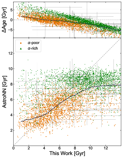
Figure 4: A comparison between age estimates for RGB stars in the APO-K2 sample produced using the method described in this work and Warfield et al. (2021) versus those produced by Mackereth et al. (2019) with AstroNN. The bottom panel compares these ages directly and the top panel shows the age offsets, $\Delta{\rm age}=\tau_{\rm NN}-\tau$. The gray, dashed line represents the one-to-one line and the blue, solid curve tracks the rolling inverse-variance weighted-mean of the data with a bin width of 2 Gyr. Orange, circular markers are stars classified as $\alpha$-poor and green, triangular markers are for $\alpha$-rich stars. In order to not overcrowd the plots, error bars are shown for a random 1% of the sample.

The comparison between our ages and the ages for the same RGB stars from Mackereth et al. (2019) is shown in Figure 4. For our sample, age versus age trends are similar to what is shown between astroNN and APOKASC-2 in Appendix A of Mackereth et al. (2019). We find that, below $\sim$4 Gyr, astroNN tends to predict ages up to $\sim$2 Gyr larger than ours, and above $\sim$8 Gyr, astroNN tends to predict lower ages, with an offset of up to 5 Gyr for the oldest stars. The astroNN ages also demonstrate a clear upper limit of approximately 10 Gyr. Similar trends have been found in other works independently deriving spectroscopic masses and ages (Martig et al. 2016; Das & Sanders 2019; Ting & Rix 2019; Anders et al. 2023; Wang et al. 2023; Stone-Martinez et al. 2023), though encouraging efforts have shown progress in addressing bias in spectroscopic ages (e.g., Ciucă et al. 2021; Leung et al. 2023).

Regarding the mismatch at old ages, the $\alpha$-rich population is known to have a very strongly peaked age distribution, which is located at $\sim$9 Gyr for the APOKASC sample when using the ages provided by Pin18. [C/N] is not strongly mass-dependent at low masses (see, e.g., Martig et al. 2016, Figure 3; Roberts et al. 2024). Therefore, algorithms relying on [C/N] are likely to assign any low-mass star to approximately the typical mass/age of an $\alpha$-rich star within random variation.

However, in general, this limitation for spectroscopic methods at old ages may not be as problematic as it initially appears. As it stands, astroNN is quite effective at tagging low-mass/old stars. War21 (as well as, e.g., Silva Aguirre et al. 2018) show that the spread in ages around the median for $\alpha$-rich stars in the Kepler field is consistent with those stars’ random age uncertainties (which we show to be the case for the K2 fields in §4.2). Similarly, the standard deviation for the $\alpha$-rich astroNN ages in Figure 4 is comparable to the spread in the APOKASC-2 $\alpha$-rich ages. The mismatch in the Figure 4 $\alpha$-rich age spread and that of K2 is driven by the larger K2 asteroseimic age uncertainties compared to APOKASC-2 (§4.2). Therefore, if it is true that the $\alpha$-rich population is approximately coeval across the Galaxy, and the APOKASC sample is the most precise measurement of this population’s age, then astroNN would be accurately predicting the age of these stars at the composite level. However, this does still rely heavily on the assumption of a coeval $\alpha$-rich population. If there are genuine, intrinsic, astrophysical trends at old ages, or a significant position–age relation at old ages, for instance, then a spectroscopic method, assigning a median $\alpha$-rich age, would be unable to uncover them.

At young ages, astroNN and other spectropic age determinations face the same limitations as the asteroseismic RGB data. That is, though the trends found from studying RGB ages may still remain (adjusted by a multiplicative zero-point, and perhaps with more random scatter than the underlying asteroseismic data set), there are still important questions to be answered regarding how well the age trends derived from RGB stars actually are reflective of, and can be applied to, the general underlying stellar population. For instance, because a star’s RGB lifetime is proportional to its MSLT, we would expect to find few young RGB stars. RC stars, with their longer lifetimes, may be a valuable tracer for the true density of younger stellar populations. Roberts et al. (2024) does show RC stars to have a more reliable [C/N]–mass relationship at high mass, potentially offering a promising avenue for tackling this question. However, today, RC stars still have limited utility, as it is difficult to put these stars on an absolute age scale due to their yet-fully understood mass loss (see Appendix B).

4 Population Analysis

4.1 K2 age distributions

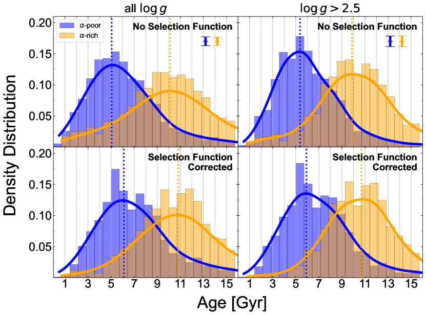
Figure 5: Density distributions for the ages of stars in the $\alpha$-poor (blue) and $\alpha$-rich (orange) RGB populations across all K2 campaigns. Densities are calculated per chemical population, such that the areas under the $\alpha$-poor and $\alpha$-rich curves histograms both, individually, sum to one, and so the relative heights of these distributions are not reflective of the relative stellar counts between each population. Along the top row, we plot these distributions for our unaltered sample and, on the bottom, for our re-scaled sample, accounting for the selection function from JSS24. The vertical, colored dashed lines mark the modal peak of each distribution. In the top right of the top panels, we show the representative Poisson uncertainties at a density of 0.1 for both the $\alpha$-poor and $\alpha$-rich sample’s histograms. The plots in the left column include stars within the full range of $\log{g}$, which includes 2176 $\alpha$-poor and 2467 $\alpha$-rich stars, where the right column is limited to the low-luminosity RGB ($\log{g}>2.5$), with 1463 $\alpha$-poor and 1402 $\alpha$-rich stars. In all panels, only stars with ${\rm[Fe/H]}<0.35$ are included, restricting the sample to the range within which our selection function can be interpolated.

For Figure 5, we have plotted one-dimensional age histograms for the $\alpha$-poor and $\alpha$-rich populations across all K2 campaigns within our sample. In the top panel, we have included all stars for which $-1.0{\rm\,dex}\leq{\rm[Fe/H]}\leq 0.35$ and $0.60{\rm\,M_{\odot}}\leq M\leq 2.6{\rm\,M_{\odot}}$, with no weighting, and in the bottom panel we have re-weighted these same stars using the Galaxia-to-K2 metallicity and mass selection function (described in §2.3). In the left column of this plot we include stars with all values of $\log{g}$, where in the right column we only include stars on the LL-RGB (§2.4).

We see, in comparing the widths of the distributions in the first row of Figure 5, that the smaller age uncertainties for the LL-RGB stars (with median age uncertainties of $\pm_{1.7}^{2.2}$ Gyrs, versus $\pm_{2.1}^{2.9}$ Gyrs for the full sample) result in correspondingly smaller spreads in the age distributions. This is perhaps more notably the case for the $\alpha$-rich population, where the standard deviation of ages for for the full sample is 5.6 Gyrs versus 4.2 Gyrs for the LL-RGB, and which is a population with considerably less intrinsic age spread versus the $\alpha$-poor population. Additionally, the percentage of very young $\alpha$-rich stars ($<4$ Gyr) in the LL-RGB sample is considerably lower (4.5% versus 8.5%). In the full catalog, there is a comparable number of stars at $<4$ Gyr as there are $>25$ Gyr. In the LL-RGB sample, there are more exceptionally young than exceptionally old stars, suggesting that the LL-RGB population of young $\alpha$-rich stars may be a purer sample of truly young or otherwise high-mass sources. However, despite these changes, the median ages of the $\alpha$-rich populations from these two samples are essentially the same (11.5 Gyrs for the full sample, 11.6 Gyrs for the LL-RGB). We suggest that this indicates that the LL-RGB represents a valid, precise subset of our sample with no biasing effect on the distributions of our populations defined by $\alpha$ abundance, and therefore we may expect the distributions from this subset to be more indicative of the intrinsic spread in ages for these populations. It also suggests that the population of young $\alpha$-rich stars may partially, but not entirely, be a product of age uncertainty (e.g., as discussed by Anders et al. 2017).

Along the bottom row of Figure 5, we see that the selection function weighted distributions are very similar to the unweighted distributions. Particular differences are that the Galaxia models seem to predict slight shifts to older ages in both populations, mainly predicting fewer very young $\alpha$-poor stars, with a larger overlap between the two populations at intermediate ages. We also see more pronounced secondary modes in both of these populations. In particular, the double-peaked profile of the $\alpha$-poor population with the selection function applied now more more closely the profile of the $\alpha$-poor population in the Kepler field (§4.2). Otherwise, the median ages of both populations agree within uncertainties.

4.2 Kepler age distributions and similarities with the K2 fields

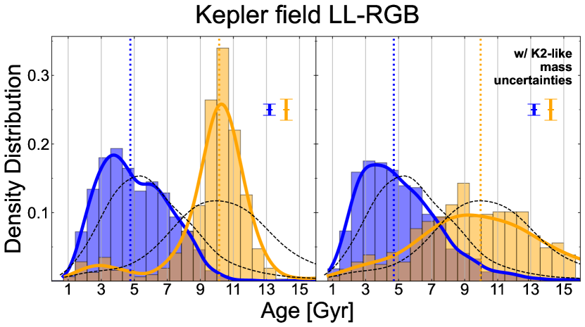
Figure 6: Density distributions for the ages of stars in the $\alpha$-poor (blue; 1557 stars) and $\alpha$-rich (orange; 452 stars) LL-RGB populations within the Kepler field. Densities are calculated per chemical population, such that the areas under the $\alpha$-poor and $\alpha$-rich histograms both, individually, sum to one, and so the relative heights of these distributions are not reflective of the relative stellar counts between each population. On the left, we plot the age distribution as it would be calculated using the methodology described in §3.1. On the right, we show the ages for the same stars calculated after those stars’ masses have been randomly perturbed randomly by the typical mass uncertainties for similar stars in the K2 fields. The dashed curves on each plot represent the KDE fits for the K2 LL-RGB sample, which is also shown in Figure 5. In the top right of each panel, we show the representative Poisson uncertainties at a density of 0.1 for both the $\alpha$-poor and $\alpha$-rich sample’s histograms.

In Figure 6, we present the age distribution for LL-RGB stars in the Kepler field. On the left, we show the ages for these stars, calculated as described in §3.1 (with masses re-calibrated from APOKASC-2, as described in §3.2). Overall, these age distributions show good agreement with those for the same sample of stars made by Silva Aguirre et al. (2018), with the primary peak of the $\alpha$-poor distribution coming in at $\sim 3$ Gyr, and the $\alpha$-rich distribution being strongly peaked at $\sim 10$ Gyr.

In comparison to the K2 sample, however, though the median ages of the $\alpha$-rich and $\alpha$-poor populations are consistent between the samples, there is still a qualitative difference in the shapes of these distributions. On the right side of Figure 6, we have plotted the age distribution of the Kepler field as it would appear if the masses of those stars had the same uncertainties as similar stars in the APO-K2 data. We have also, on both sides of the figure, plotted the distributions of the APO-K2 LL-RGB $\alpha$-poor and $\alpha$-rich samples as dashed lines. Comparing these scenarios, it seems that, by accounting for the differences in the asteroseismic mass (and, therefore, age) uncertainties between the samples, we can infer that the Kepler field’s stronger $\alpha$-rich peak and the K2 fields’ lack of a potentially double-peaked $\alpha$-poor age distribution (both seen by, e.g., Silva Aguirre et al. 2018 and Miglio et al. 2021 in the Kepler field) may be due—at least in part—to the difference in data quality between the samples (as is also noted by, e.g., Rendle et al. 2019). Inversely, we also might infer that the $\alpha$-rich stars of K2 are consistent with the $\alpha$-rich population being approximately coeval as, with K2-like uncertainties, the Kepler field’s $\alpha$-rich distribution seems to match the qualitative features of the K2 distribution, including the appearance of a potential second peak.

Despite some differences, the existing agreement between the K2 and Kepler age distributions shows the reassuring progress made with these data since War21. In War21, the authors found a median age of $\sim 8.6$ Gyrs for the $\alpha$-rich populations from Campaigns 4, 6, and 7 (K2 GAP DR2; Zinn et al. 2020), with this population having a modal age about 2 Gyrs lower than the age they found for the Kepler field. The non-astrophysical explanation given by the authors was that this was related to the overall $\nu_{\rm max}$ scaling used for K2 asteroseismic data. In K2 GAP DR2 and War21, the scaling was not tied to Gaia, and so an $\sim$2% systematic remained between the asteroseismic and astrometric radii. Using the K2 GAP DR3 data (which is calibrated to the Gaia radius scale), we now find the median age for the same set of $\alpha$-rich stars from War21 to be $\sim$20% larger, at $\sim$10.4 Gyr, which is more consistent with the age of similar stars in the Kepler field.

As we will explore in the next section, remaining discrepancies between the K2 and Kepler populations may due to real differences between stellar populations, tied to their spatial distributions across the Galaxy. Stokholm et al. (2023) similarly support this idea with age data, showing the evolution of the ages of stellar populations as a function of Galactocentric radius. This idea is also supported by Sharma et al. (2022). They compare the asteroseismic masses of the Kepler and K2 samples, both observationally and theoretically (based on Galactic models), to show that there is potentially a real difference in the modes of stellar masses across different fields independent of spectroscopic data.

4.3 Age versus Galactic position in the Kepler field and K2 fields

As we have stated above, the K2 fields are unique compared to the Kepler field because—apart from observing strategies and time baselines—they cover a much wider positional sample of the MW, both in terms of radial distance from the Galactic center ($R$) and vertical distance from the plane of the Galaxy’s disk ($Z$).

Previous studies, such as Hayden et al. (2015) using APOGEE DR12 (Holtzman et al., 2015), have already shown that both the relative and absolute distributions of stars in chemical phase-space are functions of both $R$ and $|Z|$, with, for instance, more $\alpha$-rich stars appearing at larger $|Z|$, and mostly within $R\lesssim 11$ kpc (representing the older, “thick” disk) and $\alpha$-poor stars being present at all values of $R$, but with $|Z|\lesssim 1$ kpc. In addition to these trends in the number of stars in each population, Hayden et al. (2015) observed that $\alpha$-poor stars in the range $3{\rm\,kpc}<R<5{\rm\,kpc}$ have typical [Fe/H] values of about $0.2$ dex, where stars on the outskirts of the Galaxy ($13{\rm\,kpc}<R<15{\rm\,kpc}$) have a typical [Fe/H] of about $-0.4$ dex.

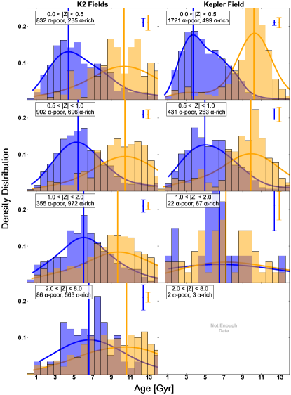
Figure 7: Density distributions for the ages of stars in the $\alpha$-poor (blue) and $\alpha$-rich (orange) RGB populations within the K2 fields (left) and Kepler field (right), in different bins of height above or below the Galactic plane, $|Z|$. Densities are calculated per chemical population, such that the areas under the $\alpha$-poor and $\alpha$-rich curves both, individually, sum to one, and so the relative heights of these distributions are not reflective of the relative stellar counts in each population. In the top right corner of each panel, we show the representative Poisson uncertainties at a density of 0.1 for both the $\alpha$-poor and $\alpha$-rich samples histograms.

Looking at both the K2 and Kepler fields, we do not see obvious trends in the age of the $\alpha$-poor population with $R$ alone. However, we do see a clear dependence on $|Z|$, which is shown in Figure 7. Similar to what was shown by War21, we see that that the peak age of the $\alpha$-poor population shifts older with increasing $|Z|$. In the K2 fields, this age is just above 4 Gyrs under 0.5 kpc, versus $\sim$6 Gyrs above 2 kpc. This seems to be connected to the bi-modal age distribution of the $\alpha$-poor population. This bi-modal distribution is most obvious in the Kepler data, where the majority of stars are at $|Z|<0.5$ kpc, and where we observe peaks in the $\alpha$-poor distribution both around 3 Gyrs and 6 Gyrs. In fact, when we look at K2 stars with $|Z|<0.5$ kpc (Figure 7, first panel), we see the younger peak emerge in this bi-modal distribution, which is not clearly present—nor dominant—when all of the data is combined. Instead, we see that, in the composite of Figure 5, this shelf in the K2 distribution is smoothed over by intermediate-age $\alpha$-poor stars, which we see (moving down the columns of Figure 7) are dominant at $|Z|>0.5$ kpc. Identically, when we look at stars in the Kepler field in the range $1{\rm\,kpc}<|Z|<2{\rm\,kpc}$, we see that the proportion of younger (versus intermediate-age) $\alpha$-poor stars has decreased, and the overall distributions in these bins more closely resemble those same bins for the K2 fields.

In Lu et al. (2022), it is shown that the $\alpha$-rich population (which we know from, e.g., Hayden et al. 2015, among others, to be more prominent at higher $|Z|$ due to being an older population that has experienced more dynamic heating) lacks a clear age-metallicity relation. Over time, stars at a given Galactic birth radius tend to be born with increasingly lower [$\alpha$/M] and higher [Fe/H] than the initial $\alpha$-rich population born at that radius. In a gas-rich environment with efficient star formation, this happens quickly, creating a radial trend in stellar metallicity distribution such that metallicities are higher in the center of the Galaxy than the exterior after the same amount of time. Then, though $\alpha$-poor stellar abundances are a function of Galactic birth radius and age, radial migration (e.g., as described by Sellwood & Binney 2002, Bland-Hawthorn et al. 2010) is sufficient to mostly wipe out the present-day radial dependence, giving rise to the $\alpha$ bi-modality (this is also discussed by, e.g., Sharma et al. 2021a). An age-$|Z|$ trend in the $\alpha$-poor population would be expected from either vertical heating mechanisms or imprinted from upside-down disc formation (e.g., Bird et al., 2021, and references therein). For our data, we seem to be seeing this same phenomenon, with a lack of strong age trends with $R$, but trends in $|Z|$ reflecting the evolution of the $\alpha$-poor sequence over time. We stress that while the age distributions of the $\alpha$-rich and $\alpha$-poor populations are typically older and younger, respectively, the $\alpha$-poor population age distribution varies with Galactic height in K2 and Kepler data. What correlations there may be in the ages of the $\alpha$-rich population with position or metallicity are not obvious with the precision afforded by either K2 or Kepler data. Ultimately, the $\alpha$ bi-modality is a multi-variate problem, which requires models that take into account metallicity- and position-dependent SFHs to begin to understand. We explore the K2 $\alpha$ bi-modality in this context in what follows.

4.4 Comparison to modeled populations

In order to test whether the predictions of various Galaxy formation theories are consistent with our data, we have compared our results to Galactic evolution and chemical enrichment models from Johnson et al. (2021). These Galactic chemical evolution models predict elemental abundances of stellar populations across the disk given two different models of the Galactic SFH. The inside-out SFH model has a generic “rise-fall” shape, while the late-burst model follows the same formalism, but with a slow Gaussian-shaped bump in the rate $\sim$2 Gyr ago (motivated by the observations of Isern 2019 and Mor et al. 2019). Stellar populations are subject to radial migration and vertical heating over their lifetimes under a prescription based on the h277 hydrodynamic simulation (e.g., Christensen et al. 2012). We refer to §2.2 and §2.5 of Johnson et al. (2021) for further details.

The product of these models is a table of stellar populations along with each population’s age, stellar mass, birth and present-day Galactic radius and height above (or below) the Galactic plane, [Fe/H], and [O/Fe]. In order to convert these data into a selection that roughly mimics our data from K2 GAP, we assigned every population of stars from the model a weight corresponding to the fraction of stars in that population that are in the mass range that would be occupied by stars on the RGB at that population’s present-day age, given the initial-mass function from Salpeter (1955). The RGB mass range was calculated assuming that a star spends $\sim$10% of its main-sequence lifetime on the RGB, and given the mass-luminosity relationship of $M\propto L^{3.8}$ (for the data from Torres et al. 2010, fit in Pinsonneault & Ryden 2023). In order to match the radial distribution of stars from the APO-K2 sample, we created bins 2 kpc wide from $R=0{\rm\,kpc}$ to $R=16{\rm\,kpc}$ and recorded the number of stars in the APO-K2 sample that fall within each of these bins, $N_{\rm bin}$. We then cut the models down to sub-samples to match the bounds of each bin in $R$, then draw $N_{\rm bin}$ populations from the sub-sample using the weights defined above. Finally, in order to produce model data sets that roughly mimic our observed sample, the abundances and ages of these populations have been randomly perturbed using the mean uncertainties for these parameters in our catalog.

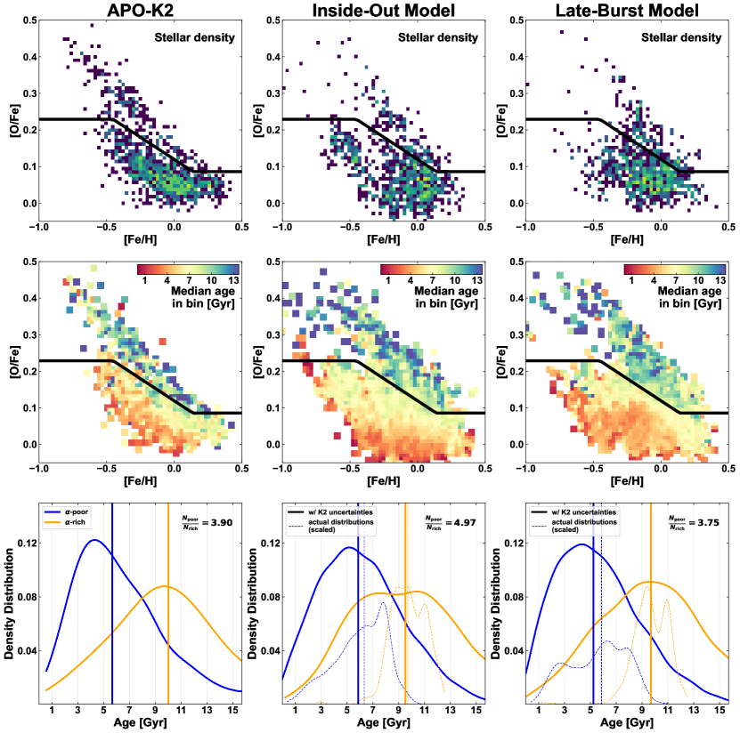
Figure 8: Top row: Number density distributions for RGB stars in the APO-K2 Catalog within 0.5 kpc of the Galactic plane compared to two models from Johnson et al. (2021): a stellar population drawn from inside-out formation models and a stellar population drawn from “late-burst” formation models in [Fe/H] vs. [O/Fe] space. The scaling is logarithmic. The black line drawn across the distributions represents the ridge-line separating the $\alpha$-rich and $\alpha$-poor populations in the K2 data. Middle row: The median age of stars within each bin in the corresponding plot on the top row. Bottom row: Age density distribution KDE curves for the $\alpha$-poor (blue) and the $\alpha$-rich (orange) populations from each respective sample. The area under the $\alpha$-poor KDE is normalized independently from the $\alpha$-rich. For the model populations, we plot the actual age distributions (i.e., ages from the models without APO-K2-like uncertainties) as dashed curves, which are normalized to fit under the solid curves. Vertical lines mark each chemical population’s median age—this does not appear for the $\alpha$-rich actual age distributions as the median is about identical to that with uncertainties. Within each panel, we give the value for the ratio of the number of $\alpha$-poor stars to the number of $\alpha$-rich stars, $N_{\rm poor}/N_{\rm rich}$. The total number of stars drawn from each model matches the number of stars in the plotted subset of APO-K2.

Histograms of the densities of the resulting populations, in [Fe/H] vs. [O/Fe] space, are shown in the top row of Figure 8 for the APO-K2 sample (left column) and the inside-out (middle column) and late-burst (right column) star formation scenarios. Here, we have only considered stars from the APO-K2 sample that are within 0.5 kpc of the Galactic plane.

One obvious difference between the models and the data from these plots is the existence of the $\alpha$ bi-modality in this chemical space; though there are arguable over-densities of $\alpha$-rich and $\alpha$-poor stars in these plots, the distinct ridge between these populations is less pronounced than it is observationally. The failure to reproduce the separation between the two sequences is a known problem with the Johnson et al. (2021) models, whereby more intermediate [O/Fe] stars are predicted than are observed (see Johnson et al. 2021, Figure 12). Despite this shortcoming, however, the models do accurately predict the observed variations in the abundance distributions between different Galactic regions. In addition to the ridge-line in the bi-modality, the $\alpha$-poor loci of these models are less constrained to a clear sequence versus the APO-K2 sample, and include additional over-densities of $\alpha$-poor stars with ${\rm[Fe/H]}\lesssim-0.5$ and $\alpha$-rich stars with ${\rm[Fe/H]}\gtrsim 0$.

Regardless of these differences, both the inside-out and late-burst models seem to do qualitatively well at matching the age distribution of stars within this chemical space (Figure 8, middle row), including an old $\alpha$-rich population with a scattered age distribution and an $\alpha$-poor population that transitions from intermediate to young ages as a function of decreasing $\alpha$ abundance. Translated to 1D histograms for the age distributions for the $\alpha$-rich and -poor populations (bottom row), we also see quantitative agreement. Considering the observational uncertainties associated with APO-K2, the median ages of these model populations are in excellent agreement with our data, and—though models do predict different proportions of stars in each of the respective chemical populations—the KDE curves seem to qualitatively resemble those of the data. Therefore, despite some remaining discrepancies between the data and models, we are unable to rule out the plausibility of either of these scenarios.

Comparing the actual, pre-perturbation age distributions from the models (plotted as dashed curves under the inside-out and late-burst data in the bottom row of Figure 8) to the ages produced when including K2-like uncertainties (solid curves in Figure 8), we see significant differences not only in the relative width of the distributions, but also in the shapes of the distributions. The age uncertainty convolution process, of course, will widen the distributions, washing out any substructure that may (or may not) be present. It will also tend to skew the distributions due to the fact that the stars have roughly constant fractional age uncertainties, not absolute age uncertainties. Nonetheless, the median age of each chemical population remains relatively unchanged after convolution, and should allow for meaningful inferences on true, population-level median ages.

5 Discussion and Conclusions

In §4.2 and §4.3, we compared the distributions of ages in the K2 and Kepler fields, and found differences in the ages between these populations are related to differences in $|Z|$ and $R$, which may be related to the generally lower mean metallicity of the Kepler sample. In fact, when we re-sample the K2 stars to reproduce the ${\rm[Fe/H]}$ distribution of the Kepler stars, we see a significant decrease in the offsets between the median ages of the populations. Re-sampling by $(R,|Z|)$ yields similar results.

Considering the relationship between the mean ${\rm[Fe/H]}$ of a given population and $(R,|Z|)$ (as shown by, e.g., Hayden et al. 2015, Imig et al. 2023), it is reasonable to assume that these two avenues of re-weighting are achieving the same ends. This relationship between chemistry and position—and the extended relationship that we have confirmed with age—demonstrates the importance of accounting for all properties of a given stellar population before applying these ages more broadly, particularly in the case of the ages of the Kepler field stars. I.e., otherwise similar stars found in different locations of the Galaxy may have different ages, which is related specifically to gradients in the SFH and the migration of stars across the Galaxy.

In §4.4, we compared the age distributions of APO-K2 stars to Johnson et al.’s (2021) Galactic chemical evolution models. Their late-burst SFH differs from their inside-out SFH only in that it includes a recent, slow burst of star formation (observationally motivated by Isern 2019 and Mor et al. 2019). Broadly, the predictions of both models are consistent with our APO-K2 sample. However, due to the substantial age uncertainties for our data, we are unable to distinguish between these models in terms of the Galaxy’s recent SFH, and, therefore, neither model can be preferred nor ruled out.

However, it is also important to note that these inside-out and late-burst models from Johnson et al. (2021) fail to fully recover the MW’s $\alpha$ bi-modality. Much has been said in the recent decades for possible histories able to produce both the kinematic and the chemical thin- and thick-disks. Clarke et al. (2019) shows that bursty episodes of brief, high star formation in simulated galaxies are able to account for both the chemical bi-modality and the associated age bi-modality of the MW. This finding seems especially promising, considering that these clumpy star-forming regions are also observed in disk galaxies at high redshift (e.g., as first identified by Cowie et al. 1995, van den Bergh et al. 1996). However, the fine-grained age predictions from this model do not agree with the data (see Clarke et al. 2019, Figure 12). On the other hand, two- and three-infall models—where the bi-modality is primarily produced by the separation of two epochs of star formation driven by distinct infall events of pristine gas into the Galaxy—have been shown capable of recovering the general age-$\alpha$ relation (Chiappini et al., 2015; Spitoni et al., 2019) and age-$Z_{\rm max}$ relation (Spitoni et al., 2022), at least as they are observed in the Kepler field/the Solar circle (using data from, e.g., Silva Aguirre et al. 2018, Ting & Rix 2019, Leung & Bovy 2019). As it stands, in-depth comparisons of the predictions of these models to those of parallel evolution models (such as those of Johnson et al. 2021) have not been done. These comparisons, done via tests of predicted age distributions as a function of chemical space with fine-grained age binning (as presented here) would place interesting constraints on the relative strengths of each class of models versus observed trends.

In this paper, we have presented precise, asteroseismically-derived ages for a large and comprehensive sample of stars in the K2 and Kepler fields. We have shown that, despite being rather ubiquitous across the Galaxy, the $\alpha$-rich and $\alpha$-poor populations show small variations in their ages that are at least partial functions of their locations in $(R,|Z|,{\rm[Fe/H]})$ phase-space. In-line with this, we conclude that nearly all of the differences that we find between the ages of $\alpha$-rich populations of the Kepler field versus the K2 fields are due to the larger uncertainties of the K2 data, and offsets in the age distribution of the $\alpha$-poor population are attributable to the differences in stellar Galactic position and metallicity between the samples. Although K2 affords a wider selection of stellar populations than Kepler, comparisons of the K2 ages against models as a function of ${\rm[\alpha/Fe]}$-${\rm[Fe/H]}$ space are not precise enough to distinguish between scenarios with versus without recent star formation. Combining Gaia distance information with TESS asteroseismology is promising for achieving more precise ages across a wide range of Galactic environment (e.g., Aguirre et al. 2020, Stello et al. 2022), which will allow for further investigations of Galactic chemical evolution models beyond the Kepler field.

Appendix A Asteroseismic Data and Catalog Pipeline

Throughout this paper, we have described our use and modifications of various published data sets, namely the APO-K2 Catalog as presented by JSS24, which itself is constructed primarily using the K2 GAP DR3 catalog (Zinn et al., 2022) and APOGEE DR17 (Abdurro’uf et al., 2022). From their origins as K2 imaging to the ages we present in this paper, these data have come together through the collective efforts of many different individuals and teams. In this appendix, we summarize the process used to build and calibrate the catalogs presented here and by JSS24.

A.1 Data processing

The K2 Galactic Archaeology Program selected red giant asteroseismic targets for K2 observations based on simple color-magnitude selection criteria, with typical K2 campaign selection criteria being (J-$\mathrm{K_{s}}$) > 0.5 and (9 < V < 15). Additional targets were selected based on previous spectroscopic identification from surveys, including APOGEE. Ultimately, more than 110,000 targets were observed from these target lists in campaigns C1-C8 and C10-C18. The selection process is discussed in more detail by Sharma et al. (2022).

Light curves were generated using EVEREST (Luger et al., 2018), which uses pixel-level data to remove systematics associated with K2’s degraded pointing compared to that of Kepler. The K2 GAP light curves were reduced and calibrated in a manner appropriate for asteroseismology, including high-pass filtering and inpainting missing data (Pires et al., 2015). Members of the Kepler Asteroseismic Science Consortium (KASC) analyzed each star, resulting in a set of asteroseismic parameters from up to six independent pipelines. The final adopted values in the K2 GAP DR3 catalog are averages of the frequency of maximum oscillation power ($\nu_{\mathrm{max}}$) and the large frequency separation ($\Delta\nu$) values across the pipelines (and campaigns, if a star was observed multiple times), with discrepant pipeline results rejected with sigma clipping (Zinn et al., 2022).

A.2 Crossmatches

To build our catalog, we started with Table 6 from Zinn et al. (2022), which has a row for each star identified by its Ecliptic Plane Input Catalog (EPIC) ID and the K2 campaign it was observed during, providing the asteroseismic $\nu_{\rm max}$ and $\Delta\nu$ values from each of the six pipelines. Each unique EPIC ID was matched to 2MASS IDs (Skrutskie et al., 2006) using the kepler.k2_epic table in the MAST Query/CasJobs database, which gives a 2MASS match for every target with an EPIC ID. These 2MASS IDs were then used to match to the APOGEE DR17 catalog, where stars are given APOGEE IDs that are equivalent to 2MASS IDs. As-is, the APOGEE catalog will have more than one entry for some 2MASS IDs due to the same source being targeted in distinct observing programs. In order to assure a one-to-one crossmatch, we first sorted the APOGEE table by SNR, then dropped the duplicate 2MASS entries with the lower SNR value. From this crossmatched table, we removed all objects for which there was no measured $\nu_{\rm max}$, $\Delta\nu$, or [Fe/H].

A.3 $\Delta\nu$ and $\nu_{\rm max}$ Calibration

Asteroseismic masses and radii are calculated according to scaling relations following the notation of Sharma et al. (2016):

$$\frac{M}{M_{\odot}}\approx\left(\frac{\nu_{\rm max}}{f_{\nu_{\rm max}}\nu_{\rm max,\odot}}\right)^{3}\left(\frac{\Delta\nu}{f_{\Delta\nu}\Delta\nu_{\odot}}\right)^{-4}\left(\frac{T_{\rm eff}}{T_{\rm eff,\odot}}\right)^{3/2}\equiv\kappa_{M}\left(\frac{T_{\rm eff}}{T_{\rm eff,\odot}}\right)^{3/2},$$ (A1)

$$\frac{R}{R_{\odot}}\approx\left(\frac{\nu_{\rm max}}{f_{\nu_{\rm max}}\nu_{\rm max,\odot}}\right)\left(\frac{\Delta\nu}{f_{\Delta\nu}\Delta\nu_{\odot}}\right)^{-2}\left(\frac{T_{\rm eff}}{T_{\rm eff,\odot}}\right)^{1/2}\equiv\kappa_{R}\left(\frac{T_{\rm eff}}{T_{\rm eff,\odot}}\right)^{1/2}.$$ (A2)

These scaling relations are approximations linked to solar values and require calibration factors, $f_{\Delta\nu}$ and $f_{\nu_{\mathrm{max}}}$, because $\Delta\nu$ does not scale exactly as stellar mean density (White et al., 2011) and $\nu_{\rm max}$ does not scale exactly as g/$T_{\rm eff}$ (Brown et al., 1991; Kjeldsen & Bedding, 1995). These calibration factors vary by star and depend on, in part, the star’s temperature and metallicity.

For APO-K2, we used APOGEE DR17 temperatures and metallicities to update $f_{\Delta\nu}$ using Asfgrid (Sharma et al., 2016) with the low-mass, low-metallicity extension (Stello & Sharma, 2022). Specifically, we used Asfgrid to perform a multi-dimensional interpolation of $f_{\Delta\nu}$ using evolutionary state (see below), a Salaris-corrected metallicity using APOGEE [$\alpha$/M] (Salaris et al., 1993), APOGEE temperature, $\Delta\nu$, and $\nu_{\rm max}$.

The K2 GAP DR3 asteroseismic data that feed into the APO-K2 catalog were additionally calibrated using Gaia parallaxes inferred from bulk stellar motions from Gaia DR2 (Gaia Collaboration et al., 2018) according to the methodology detailed in Schönrich et al. (2019) and accounting for selection functions according to Schönrich & Aumer (2017). This technique corrects for parallax bias, and indicates $\sim 10$ $\mu$as positional variations in the Gaia parallax zero-point across K2 campaigns. The resulting Gaia parallaxes were then compared to asteroseismic parallaxes, which can be computed from asteroseismic radii in combination with the Stefan-Boltzmann law. $f_{\nu_{\mathrm{max}}}$ was defined to bring the asteroseismic parallaxes into agreement with the Gaia parallaxes. A separate value was computed for RGB and RC stars, in recognition of their different stellar structure (and therefore potentially different asteroseismic systematics) as well as their potentially different selection functions (and therefore potentially different Gaia parallax systematics).

A.4 Evolutionary States

With a long enough time baseline, the evolutionary state of stars can be determined directly through an asteroseismic analysis of light curves (e.g., Bedding et al. 2011). Though this is possible for the original Kepler/APOKASC data (e.g.; Pin18; Elsworth et al. 2019; M. Pinsonneault et al. 2024, in preparation 2024), and some work has been done on doing the same light curve analysis for shorter-baseline data using neural networks (e.g., Hon et al. 2018), these methods are still far from ideal for the relatively noisy K2 data.

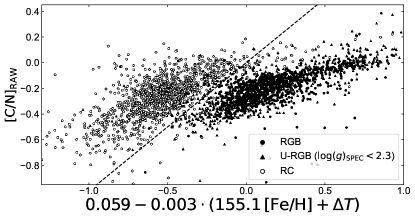
Figure 9: A random sample of asteroseismically-classified RGB (filled) and RC (unfilled) stars from the APOKASC-3 catalog, plotted in the space of the spectroscopic fit. The $y$-axis is the uncalibrated APOGEE [C/N] and the $x$-axis is an empirical surface gravity- and metallicity-dependent parameter (see text for details). Stars with low surface gravities and therefore assumed to be RGB/AGB stars spectroscopically are also shown. The dashed line is one-to-one, under which stars would be spectroscopically classified as RGB and above RC.

An alternative is to determine the evolutionary states of stars spectroscopically using cuts in temperature, surface gravity, and element abundances (specifically, [Fe/H] and [C/N]; e.g., Bovy et al. 2014, Elsworth et al. 2019). To do this, we first define a “reference” temperature, which is defined as the typical effective temperature we would expect for an RGB of a given metallicity and surface gravity:

$$T_{\rm ref}=\alpha+\beta\,{\rm[Fe/H]_{\rm RAW}}+\gamma\,(\log(g)_{\rm SPEC}-2.5).$$ (A3)

Spectroscopic parameters are taken from APOGEE DR17, and $\alpha$, $\beta$, and $\gamma$ are fit parameters that are determined through a nonlinear least-squares fit for stars classified as RGB in the APOKASC-3 catalog. After determining these values ($\alpha=4427.1779$, $\beta=-399.5105$, $\gamma=553.1705$), a Monte Carlo optimization is used to find values for $a$, $b$, and $c$ in a second expression:

$$a-b\,(c\,{\rm[Fe/H]_{\rm RAW}}+T_{\rm eff}^{\rm SPEC}-T_{\rm ref})-{\rm[C/N]_{\rm RAW}},$$ (A4)

for which at least 98% of stars with a value less than 0 have an asteroseismic RGB classification (Figure 9). We found best-fit values of $a=0.05915$, $b=0.003455$, and $c=155.1$. This expression is then applied to our APO-K2 data set, assigning all stars for which A4 $<0$ as RGB and $>0$ as RC. The exception is for stars on the upper-RGB (U-RGB), which we have conservatively defined as $\log(g)<2.3$. These stars fall in a region of a Kiel diagram beyond what is possible for the RC, and so have all been classified as RGB, regardless of their value for A4.

A.5 Selection Function

Due to being the product of a cross-match between K2 GAP and APOGEE DR17, the APO-K2 catalog is subject to selection and targeting choices made by both of these surveys. By understanding the selection function of the underlying samples, JSS24 assessed the completeness of the sample and existing effects on the distributions of stellar parameters by comparing the selection function for the whole APO-K2 sample to that of K2 GAP. This selection function is defined in bins of mass and stellar metallicity, giving the ratio of the number of stars in the APO-K2 sample versus the K2 GAP sample for each bin. These ratios can then be used as weights when analyzing the APO-K2 sample.

This same comparison is also done between the APO-K2 sample and a set of simulated stars drawn from a parent mock Galactic asteroseismic red giant population generated with Galaxia (Sharma et al., 2011). These simulated stars are drawn in color and magnitude space in accordance with the original K2 GAP targeting selection function, and then have an expected asteroseismic selection function applied in order to only retain stars with a $>90\%$ probability of having detectable asteroseismic signals (Sharma et al., 2022).

A.6 Ages

Our ages in this paper use the methodology and code that some of these authors first presented in War21. Each star is defined by its values for $\log({\rm Mass})$ (from asteroseismology), [Fe/H] and [$\alpha$/M] (from APOGEE DR17), and the 1$\sigma$ uncertainties for each of these, which are then used as look-up parameters in a regular four-dimensional grid—including $\log({\rm age})$—constructed from sets of stellar evolutionary tracks.

Our stellar evolutionary tracks were generated originally by/for Tayar et al. (2017) using the Yale Rotating Evolution Code (Pinsonneault et al., 1989; van Saders & Pinsonneault, 2012). Given tabulated values for stellar mass, present-day surface element abundances, surface gravity, and temperature, these tracks provide the age of a star when leaving the main sequence/joining the RGB (the MSLT). From these tracks, we created three sets of grids at fixed $\log(g)$ values of 3.30, 2.50, and 1.74 (chosen as discrete values in the tracks that approximately separate and bracket the low-luminosity giants from the luminous giants), and assuming a solar He abundance of 0.272683 and solar mixing length of 1.72. These grids are tabulated at mass values between 0.6 M_⊙ and 2.6 M_⊙, with 0.1 M_⊙ steps; [Fe/H] values between -2.0 and 0.6, with 0.2 dex steps; and [$\alpha$/M] values of 0.0, 0.2, and 0.4.

We chose this approach because the MSLT is well-defined as a function of mass. The age of a star at a specific location on the RGB requires at least accounting for $T_{\rm eff}$, which is strongly correlated to age in this regime. However, this also leads to small uncertainties in temperature (or systematic offsets between model and data zero-points) being associated with large swings in age, with a 50 K uncertainty in $T_{\rm eff}$ (typical of the APOGEE data) corresponding to an $\sim 70\%$ uncertainty in age (Tayar et al. 2017, War21). For these reasons, and considering also that the amount of time spent on the RGB ($\sim 10\%$ of the MSLT) is smaller than our stellar age uncertainties (even for the APOKASC sample), the MSLT, as determined via mass, serves as a very consistent age measurement across both asteroseismic samples.

Given values of $(x,y,z)\equiv(\log{M},{\rm[Fe/H]},{\rm[\alpha/M]})$, we can then find an associated value for $w\equiv\log({\rm age})$ from our model grid via four-point, four-dimensional Lagrange interpolation. In two dimensions, four-point Lagrange interpolation works by constructing a Lagrange interpolation polynomial of the form:

$$L(x)=\sum_{j=0}^{3}w_{j}l_{j}(x),$$ (A5)

where

$$l_{j}(x)=\prod_{0\leq m\leq 3\atop m\neq j}\frac{x-x_{m}}{x_{j}-x_{m}}$$ (A6)

are the Lagrange basis polynomials. For a set of four ordered pairs $(x_{0},w_{0}),...,(x_{3},w_{3})$, this equation gives an estimate for values of $w=L(x)$ for any given $x\in(x_{0},x_{3})$ while keeping that $L(x_{j})=w_{j}$. Expanded to four-dimensions, this then becomes:

$$L(x,y,z)=\sum_{j=0}^{3}\sum_{k=0}^{3}\sum_{m=0}^{2}w_{j,k,m}l_{j}(x)l_{k}(y)l_{m}(z).$$ (A7)

Using a Monte Carlo method to produce 5,000 $(x,y,z)$ tuples for each star (assuming a Gaussian error distribution for each parameter), we then used Equation A7 to make two $\log({\rm age})$ estimates for each tuple, one with each of the tracks for the $\log{g}$ values that bracket the input star’s $\log{g}$. For this calculation, four nearest-neighbor points were chosen from the model grid so that, for each parameter, $x_{0}<x_{1}<x<x_{2}<x_{3}$. The exception is for $z\equiv{\rm[\alpha/M]}$ where, since the tracks from Tayar et al. (2017) only sample three values of [$\alpha$/M], $(z_{0},z_{1},z_{3})=(0.0,0.2,0.4)$ always, and so the associated basis polynomial, $l_{m}(z)$, is always constructed using these points.

After obtaining 5,000 $\log({\rm age})$ estimates, the median and $\pm 1\sigma$ were calculated in $\log$ space for each grid, and then converted to linear space for tabulation. The mean of the low- and high-$\log{g}$ grid values is used, with the difference between them added as a systematic error. However, in all cases, there is no offset between these two values.

Appendix B Ages on the Red Clump

In §2.4, we explain our reasoning for only considering RGB stars as being due to the mass loss in the RC not being fully understood, leading to biases in the ages of these stars (e.g., Casagrande et al., 2016). This issue could theoretically be resolved with a prescription for this mass loss. However, it is not clear how—if at all—mass loss on the RGB is related to stellar age or abundance (An et al., 2019). Absent a physics-driven understanding of mass loss that is applicable to stars on an individual basis, it may instead be possible to characterize this bias empirically for a given population. For instance, we might assume that the mean mass (or age) of $\alpha$-rich RC stars in the APO-K2 sample should be the same as that of the $\alpha$-rich RGB stars, and therefore apply the multiplicative offset between the means to each star’s mass (or age) ex post facto. However, this would grant these stars very limited utility: there would be little reason to trust the “corrected” age of individual stars, and it would be difficult to separate genuine features of the age profile from a mis-accounting of mass loss. Regardless, this may still be an intriguing avenue for generally characterizing the expected magnitude of this change.

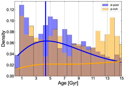
Figure 10: Age distributions for the 2298 $\alpha$-poor and 1357 $\alpha$-rich RC stars in the APO-K2 sample. These ages have been estimated using present day asteroseismic masses, uncorrected for potential mass loss.

Table 3: The partial data table for the APO-K2 RC sample, including our ages. The complete table is available in CSV format in the online journal. The main identifier for each star is its ID in the Ecliptic Plane Input Catalog (EPIC). In addition to the columns shown here, our table contains Galactic longitude and latitudes; Galactocentric $R$ and $Z$ positions; the uncalibrated values for APOGEE $T_{\rm eff}$, $\log{g}$, [Fe/H], [$\alpha$/M], and [O/Fe], as well as the associated errors for all relevant columns. The $\alpha$-rich Flag column has a value of 1 for $\alpha$-rich stars, 0 for $\alpha$-poor stars, and -1 for unclassified stars.

EPIC ID	APOGEE ID	Gaia EDR3 Source ID	RA	DEC	$T_{\rm eff}$	$\log(g)_{\rm APO}$	[Fe/H]	[$\alpha$/M]	[O/Fe]	$\alpha$-rich Flag	Mass	Radius	$\log(g)_{\rm seis}$	$\nu_{\rm max}$	$\Delta\nu$	Age	Modal Age
			(Deg.)	(Deg.)	(K)	($\log({\rm cm/s}^{2})$)	(dex)	(dex)	(dex)		(M⊙)	(R⊙)	($\log({\rm cm/s}^{2})$)	($\mu$Hz)	($\mu$Hz)	(Gyr)	(Gyr)
212532733	2M13122093$-$1202115	3621787595338351872	198.0872	-12.0366	4644	2.25	-0.296	0.220	0.307		0.77	11.33	2.21	20.4	3.10	28.2	27.5
211163406	2M03582817$+$2541126	67156795835480448	59.6174	25.6869	4616	2.45	-0.060	0.037	0.065		1.22	10.70	2.46	36.6	4.26	5.7	5.1
212451149	2M13180826$-$1346410	3609158841003939968	199.5344	-13.7781	4925	2.55	-0.239	0.043	0.060		1.15	9.83	2.51	39.5	4.69	5.9	5.4
210618287	2M04235747$+$1713227	3313965708686969728	65.9895	17.2230	4438	2.21	-0.059	0.073	0.108		1.10	12.27	2.30	25.7	3.30	8.4	7.9
212750556	2M13191487$-$0657577	3634414902267654400	199.8120	-6.9660	4264	1.93	-0.059	0.107	0.147		1.24	19.06	1.97	12.2	1.81	5.5	3.7
204987895	2M16111595$-$1956386	6245469248293963648	242.8165	-19.9441	4556	2.12	-0.411	0.154	0.199		0.89	12.54	2.19	19.7	2.88	13.4	10.2
205170082	2M16384287$-$1903121	4131201704833326592	249.6786	-19.0534	4817	2.52	-0.018	0.020	0.025		1.13	9.85	2.51	39.4	4.65	7.3	7.2
220637427	2M00504808$+$0952289	2582124996801990528	12.7003	9.8747	4618	2.52	-0.304	0.235	0.275		0.99	9.31	2.49	39.1	4.72	11.0	11.1
246144695	2M23021866$-$0610311	2634924193707214080	345.5778	-6.1753	4586	2.08	-0.383	0.109	0.134		0.96	13.59	2.15	18.0	2.65	10.3	10.5
…	…	…	…	…	…	…	…	…	…		…	…	…	…	…	…	…

In Figure 10, we have plotted the age distributions for the $\alpha$-poor and $\alpha$-rich populations of RC stars in the APO-K2 catalog, calculated without any correction for mass loss. In one sense, these ages may still be useful. We see a slight peak in $\alpha$-rich ages at $\sim$14 Gyrs, and a gradual peak of younger $\alpha$-poor stars. However, the main difference between these ages and those for the RGB stars is that there are many more $\alpha$-rich RC stars at intermediate and young ages. Still, it is possible that this is telling us something real about these populations. For instance, we would expect more RC stars to go through mergers, and one possible explanation for the young $\alpha$-rich population (that is also observed among the RGB stars) is that these are merger products that have larger present-day masses than they had at birth, and so they are interpreted as being younger than they actually are (Chiappini et al., 2015; Martig et al., 2015). These ages can be found in Table 3, though we strongly encourage readers to pay heed to the limitations we have highlighted above and to exercise caution when using these data.

Appendix C Ages for Metal Poor Stars

Thus far, we have excluded metal poor stars from our analysis due to significant uncertainty in the calibration of the asteroseismic scaling relations at ${\rm[Fe/H]}\lesssim-1$, which, in turn, leads to systematic overestimates in the masses of these stars. Epstein et al. (2014) notably presented this issue using APOKASC-1 data, showing an $\sim$10% overestimate for the asteroseismic masses of halo stars as compared to model predictions. Subsequent studies have shown mixed levels of systematics (see JSS24 and references therein).

Table 4: The partial data table for the stars in the APO-K2 sample with ${\rm[Fe/H]}<-1$, including our ages, which have their masses calibrated and calculated using the uncalibrated APOGEE $T_{\rm eff}$ values. The complete table is available in CSV format in the online journal. The main identifier for each star is its ID in the Ecliptic Plane Input Catalog (EPIC). In addition to the columns shown here, our table contains Galactic longitude and latitudes; Galactocentric $R$ and $Z$ positions; the uncalibrated values for APOGEE [Fe/H], [$\alpha$/M], and [O/Fe], as well as the associated errors for all relevant columns. The $\alpha$-rich Flag column is not populated for these stars, as the $\alpha$-rich and $\alpha$-poor populations are not well defined at these metallicities, though it may be assumed that these stars are more similar to the $\alpha$-rich population.

EPIC ID	APOGEE ID	Gaia EDR3 Source ID	RA	DEC	$T_{\rm eff}^{\rm uncal.}$	$\log(g)_{\rm APO}^{\rm uncal.}$	[Fe/H]	[$\alpha$/M]	[O/Fe]	Mass	Radius	$\log(g)_{\rm seis}$	$\nu_{\rm max}$	$\Delta\nu$	Age	Modal Age
			(Deg.)	(Deg.)	(K)	($\log({\rm cm/s}^{2})$)	(dex)	(dex)	(dex)	(M⊙)	(R⊙)	($\log({\rm cm/s}^{2})$)	($\mu$Hz)	($\mu$Hz)	(Gyr)	(Gyr)
212498924	2M13181597$-$1245237	3609527147335455744	199.5666	-12.7566	4729	1.55	-1.908	0.199	0.680		13.72	2.07	14.4	2.38	11.3	8.6
201226802	2M12005757$-$0333311	3600860727964887680	180.2399	-3.5587	4567	1.70	-1.172	0.242	0.323		15.73	1.94	11.0	1.92	13.4	9.9
228946727	2M12390889$-$0227021	3682958718591170560	189.7870	-2.4506	4849	2.09	-1.814	0.218	0.186		7.17	2.64	53.1	6.35	11.9	11.0
251545861	2M13223901$-$0228562	3638105756643622912	200.6626	-2.4823	4766	2.17	-1.075	0.207	0.574		10.01	2.33	26.4	3.77	14.4	13.0
211480777	2M08441675$+$1251409	602285256783119616	131.0698	12.8614	4598	1.81	-1.038	0.159	0.409		18.97	1.92	10.4	1.71	4.4	4.2
216439618	2M18540793$-$2220424	4078727070039971968	283.5331	-22.3451	4894	2.16	-1.401	0.344	0.018		9.99	2.23	20.7	3.36	31.9	29.8
212510240	2M13171736$-$1230546	3609593083673337472	199.3223	-12.5152	4517	1.77	-1.031	0.274	0.383		15.33	1.92	10.5	1.90	21.4	18.8
203520011	2M16110245$-$2551498	6043468754447485696	242.7602	-25.8638	4706	2.11	-1.144	0.315	0.500		9.12	2.35	27.7	4.04	24.5	22.0
211326502	2M08550079$+$1022483	597826737133200256	133.7533	10.3801	5033	2.73	-1.200	0.352	0.483		5.83	2.86	88.0	9.15	9.4	9.1
…	…	…	…	…	…	…	…	…	…		…	…	…	…	…	…

Table 4 contains all stars (230) from the APO-K2 catalog with ${\rm[Fe/H]}<-1$. All of these stars are assumed to be RGB stars, as no RC stars should exist in this metallicity range. The masses (and, thereby, ages) of these stars have been calculated using the uncalibrated temperatures from APOGEE, which are those inferred from fitting to a grid of synthetic spectra generated by the spectral synthesis code Turbospectrum (Alvarez & Plez, 1998; Plez, 2012) under 1D local thermodynamic equilibrium. These temperatures are shown by JSS24 to produce masses more in-line with what is expected for halo populations from stellar isochrones, though a mean offset of up to $\approx 10\%$ may remain.

Appendix D Per-Campaign Age Distributions

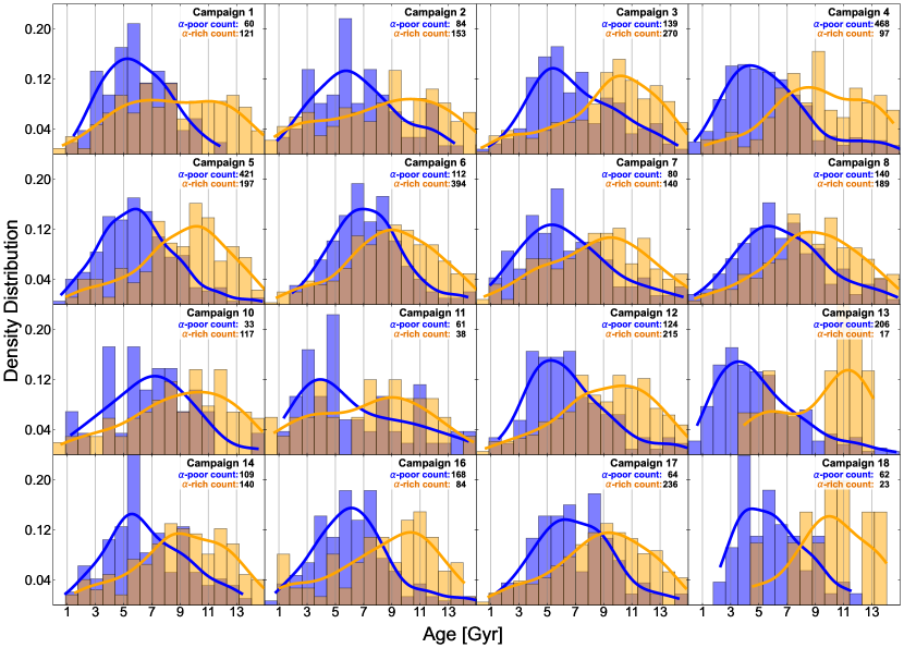
Figure 11: Density distributions for the ages of stars in the $\alpha$-poor (blue) and $\alpha$-rich (orange) RGB populations, split up by K2 campaign. Excluded is Campaign 15, for which we were only able to recover ages for 3 RGB stars. Densities are calculated per chemical population, such that the areas under the $\alpha$-poor and $\alpha$-rich curves both, individually, sum to one, and so the relative heights of these distributions are not reflective of the relative stellar counts in each field. Embedded in the plot, we have also included the number of stars per chemical population per campaign.

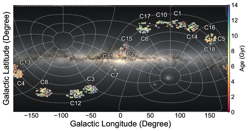
Figure 12: Map of the K2 Campaigns by Galactic Longitude and Latitude. Each point represents an individual star, with each point being colored by age. The background image is modified from ESA/Gaia/DPAC, and is applied using the mwplot Python module and the MWSkyProjection map “equirectangular”.

In Figure 11, we show histograms for the age distributions of the $\alpha$-rich and $\alpha$-poor populations, separated by campaign. In Figure 12, we map these campaigns on the sky, colored by age.

References

- Abdurro’uf et al. (2022) Abdurro’uf, Accetta, K., Aerts, C., et al. 2022, ApJS, 259, 35, doi: 10.3847/1538-4365/ac4414
- Aguirre et al. (2020) Aguirre, V. S., Stello, D., Stokholm, A., et al. 2020, ApJ, 889, L34
- Aller & Greenstein (1960) Aller, L. H., & Greenstein, J. L. 1960, ApJS, 5, 139
- Alvarez & Plez (1998) Alvarez, R., & Plez, B. 1998, A&A, 330, 1109
- An et al. (2019) An, D., Pinsonneault, M. H., Terndrup, D. M., & Chung, C. 2019, ApJ, 879, 81, doi: 10.3847/1538-4357/ab23ed
- Anders et al. (2017) Anders, F., Chiappini, C., Rodrigues, T. S., et al. 2017, A&A, 597, A30, doi: 10.1051/0004-6361/201527204
- Anders et al. (2023) Anders, F., Gispert, P., Ratcliffe, B., et al. 2023, A&A, 678, A158, doi: 10.1051/0004-6361/202346666
- Astropy Collaboration et al. (2013) Astropy Collaboration, Robitaille, T. P., Tollerud, E. J., et al. 2013, A&A, 558, A33, doi: 10.1051/0004-6361/201322068
- Astropy Collaboration et al. (2018) Astropy Collaboration, Price-Whelan, A. M., Sipőcz, B. M., et al. 2018, AJ, 156, 123, doi: 10.3847/1538-3881/aabc4f
- Astropy Collaboration et al. (2022) Astropy Collaboration, Price-Whelan, A. M., Lim, P. L., et al. 2022, ApJ, 935, 167, doi: 10.3847/1538-4357/ac7c74
- Baglin (2003) Baglin, A. 2003, Advances in Space Research, 31, 345, doi: 10.1016/S0273-1177(02)00624-5
- Bailer-Jones (2015) Bailer-Jones, C. A. L. 2015, PASP, 127, 994
- Beaton et al. (2021) Beaton, R. L., Oelkers, R. J., Hayes, C. R., et al. 2021, AJ, 162, 302, doi: 10.3847/1538-3881/ac260c
- Bedding et al. (2011) Bedding, T. R., Mosser, B., Huber, D., et al. 2011, Nature, 471, 608
- Bensby et al. (2003) Bensby, T., Feltzing, S., & Lundström, I. 2003, A&A, 410, 527
- Bird et al. (2021) Bird, S. A., Xue, X.-X., Liu, C., et al. 2021, ApJ, 919, 66
- Bland-Hawthorn et al. (2010) Bland-Hawthorn, J., Krumholz, M. R., & Freeman, K. 2010, ApJ, 713, 166, doi: 10.1088/0004-637X/713/1/166
- Blanton et al. (2017) Blanton, M. R., Bershady, M. A., Abolfathi, B., et al. 2017, AJ, 154, 28, doi: 10.3847/1538-3881/aa7567
- Borucki et al. (2010) Borucki, W. J., Koch, D., Basri, G., et al. 2010, Science, 327, 977
- Bovy et al. (2012) Bovy, J., Rix, H.-W., & Hogg, D. W. 2012, ApJ, 751, 131, doi: 10.1088/0004-637X/751/2/131
- Bovy et al. (2014) Bovy, J., Nidever, D. L., Rix, H.-W., et al. 2014, ApJ, 790, 127
- Bowen & Vaughan (1973) Bowen, I. S., & Vaughan, A. H. 1973, Appl. Opt., 12, 1430
- Brown et al. (1991) Brown, T. M., Gilliland, R. L., Noyes, R. W., & Ramsey, L. W. 1991, ApJ, 368, 599
- Casagrande et al. (2016) Casagrande, L., Silva Aguirre, V., Schlesinger, K. J., et al. 2016, MNRAS, 455, 987
- Chiappini et al. (1997) Chiappini, C., Matteucci, F., & Gratton, R. 1997, ApJ, 477, 765, doi: 10.1086/303726
- Chiappini et al. (2015) Chiappini, C., Anders, F., Rodrigues, T. S., et al. 2015, A&A, 576, L12
- Chieffi & Straniero (1989) Chieffi, A., & Straniero, O. 1989, ApJS, 71, 47, doi: 10.1086/191364
- Christensen et al. (2012) Christensen, C., Quinn, T., Governato, F., et al. 2012, MNRAS, 425, 3058, doi: 10.1111/j.1365-2966.2012.21628.x
- Ciucă et al. (2021) Ciucă, I., Kawata, D., Miglio, A., Davies, G. R., & Grand, R. J. J. 2021, MNRAS, 503, 2814, doi: 10.1093/mnras/stab639
- Clarke et al. (2019) Clarke, A. J., Debattista, V. P., Nidever, D. L., et al. 2019, MNRAS, 484, 3476
- Cowie et al. (1995) Cowie, L. L., Hu, E. M., & Songaila, A. 1995, AJ, 110, 1576, doi: 10.1086/117631
- Cui et al. (2012) Cui, X.-Q., Zhao, Y.-H., Chu, Y.-Q., et al. 2012, Research in Astronomy and Astrophysics, 12, 1197, doi: 10.1088/1674-4527/12/9/003
- Das & Sanders (2019) Das, P., & Sanders, J. L. 2019, MNRAS, 484, 294, doi: 10.1093/mnras/sty2776
- De Silva et al. (2015) De Silva, G. M., Freeman, K. C., Bland-Hawthorn, J., et al. 2015, MNRAS, 449, 2604, doi: 10.1093/mnras/stv327
- Elsworth et al. (2019) Elsworth, Y., Hekker, S., Johnson, J. A., et al. 2019, MNRAS, 489, 4641
- Epstein et al. (2014) Epstein, C. R., Elsworth, Y. P., Johnson, J. A., et al. 2014, ApJ, 785, L28
- Gaia Collaboration et al. (2016) Gaia Collaboration, Prusti, T., de Bruijne, J. H. J., et al. 2016, A&A, 595, A1
- Gaia Collaboration et al. (2018) Gaia Collaboration, Brown, A. G. A., Vallenari, A., et al. 2018, A&A, 616, A1
- Gaia Collaboration et al. (2023) Gaia Collaboration, Vallenari, A., Brown, A. G. A., et al. 2023, A&A, 674, A1, doi: 10.1051/0004-6361/202243940
- Gilmore & Reid (1983) Gilmore, G., & Reid, N. 1983, MNRAS, 202, 1025
- Grevesse & Sauval (1998) Grevesse, N., & Sauval, A. J. 1998, Space Sci. Rev., 85, 161, doi: 10.1023/A:1005161325181
- Gunn et al. (2006) Gunn, J. E., Siegmund, W. A., Mannery, E. J., et al. 2006, AJ, 131, 2332
- Hayden et al. (2015) Hayden, M. R., Bovy, J., Holtzman, J. A., et al. 2015, ApJ, 808, 132
- Haywood et al. (2013) Haywood, M., Di Matteo, P., Lehnert, M. D., Katz, D., & Gómez, A. 2013, A&A, 560, A109
- Holtzman et al. (2015) Holtzman, J. A., Shetrone, M., Johnson, J. A., et al. 2015, AJ, 150, 148, doi: 10.1088/0004-6256/150/5/148
- Holtzman et al. (2018) Holtzman, J. A., Hasselquist, S., Shetrone, M., et al. 2018, AJ, 156, 125
- Hon et al. (2018) Hon, M., Stello, D., & Yu, J. 2018, MNRAS, 476, 3233, doi: 10.1093/mnras/sty483
- Howell et al. (2014) Howell, S. B., Sobeck, C., Haas, M., et al. 2014, PASP, 126, 398
- Iglesias & Rogers (1996) Iglesias, C. A., & Rogers, F. J. 1996, ApJ, 464, 943, doi: 10.1086/177381
- Imig et al. (2023) Imig, J., Price, C., Holtzman, J. A., et al. 2023, ApJ, 954, 124
- Isern (2019) Isern, J. 2019, ApJ, 878, L11, doi: 10.3847/2041-8213/ab238e
- Johnson et al. (2021) Johnson, J. W., Weinberg, D. H., Vincenzo, F., et al. 2021, MNRAS, 508, 4484, doi: 10.1093/mnras/stab2718
- Jönsson et al. (2020) Jönsson, H., Holtzman, J. A., Allende Prieto, C., et al. 2020, AJ, 160, 120
- Kjeldsen & Bedding (1995) Kjeldsen, H., & Bedding, T. R. 1995, A&A, 293, 87
- Kobayashi et al. (1998) Kobayashi, C., Tsujimoto, T., Nomoto, K., Hachisu, I., & Kato, M. 1998, ApJ, 503, L155
- Leung & Bovy (2019) Leung, H. W., & Bovy, J. 2019, MNRAS, 483, 3255, doi: 10.1093/mnras/sty3217
- Leung et al. (2023) Leung, H. W., Bovy, J., Mackereth, J. T., & Miglio, A. 2023, MNRAS, 522, 4577, doi: 10.1093/mnras/stad1272
- Lindegren et al. (2021) Lindegren, L., Bastian, U., Biermann, M., et al. 2021, A&A, 649, A4, doi: 10.1051/0004-6361/202039653
- Lu et al. (2022) Lu, Y., Minchev, I., Buck, T., et al. 2022, arXiv e-prints, arXiv:2212.04515, doi: 10.48550/arXiv.2212.04515
- Luger et al. (2018) Luger, R., Kruse, E., Foreman-Mackey, D., Agol, E., & Saunders, N. 2018, AJ, 156, 99
- Mackereth et al. (2019) Mackereth, J. T., Bovy, J., Leung, H. W., et al. 2019, MNRAS, 489, 176, doi: 10.1093/mnras/stz1521
- Majewski et al. (2017) Majewski, S. R., Schiavon, R. P., Frinchaboy, P. M., et al. 2017, AJ, 154, 94
- Martig et al. (2015) Martig, M., Rix, H.-W., Silva Aguirre, V., et al. 2015, MNRAS, 451, 2230
- Martig et al. (2016) Martig, M., Fouesneau, M., Rix, H.-W., et al. 2016, MNRAS, 456, 3655, doi: 10.1093/mnras/stv2830
- Miglio et al. (2021) Miglio, A., Chiappini, C., Mackereth, J. T., et al. 2021, A&A, 645, A85, doi: 10.1051/0004-6361/202038307
- Mor et al. (2019) Mor, R., Robin, A. C., Figueras, F., Roca-Fàbrega, S., & Luri, X. 2019, A&A, 624, L1, doi: 10.1051/0004-6361/201935105
- Mosser et al. (2013) Mosser, B., Dziembowski, W. A., Belkacem, K., et al. 2013, A&A, 559, A137
- Nidever et al. (2015) Nidever, D. L., Holtzman, J. A., Allende Prieto, C., et al. 2015, AJ, 150, 173
- Pinsonneault & Ryden (2023) Pinsonneault, M., & Ryden, B. 2023, Stellar Structure and Evolution (Cambridge University Press), doi: 10.1017/9781108869249
- Pinsonneault et al. (1989) Pinsonneault, M. H., Kawaler, S. D., Sofia, S., & Demarque, P. 1989, ApJ, 338, 424
- Pinsonneault et al. (2018) Pinsonneault, M. H., Elsworth, Y. P., Tayar, J., et al. 2018, ApJS, 239, 32
- Pires et al. (2015) Pires, S., Mathur, S., García, R. A., et al. 2015, A&A, 574, A18
- Plez (2012) Plez, B. 2012, Turbospectrum: Code for spectral synthesis, Astrophysics Source Code Library, record ascl:1205.004
- Prochaska et al. (2000) Prochaska, J. X., Naumov, S. O., Carney, B. W., McWilliam, A., & Wolfe, A. M. 2000, AJ, 120, 2513
- Rendle et al. (2019) Rendle, B. M., Miglio, A., Chiappini, C., et al. 2019, MNRAS, 490, 4465, doi: 10.1093/mnras/stz2454
- Ricker et al. (2015) Ricker, G. R., Winn, J. N., Vanderspek, R., et al. 2015, Journal of Astronomical Telescopes, Instruments, and Systems, 1, 014003, doi: 10.1117/1.JATIS.1.1.014003
- Roberts et al. (2024) Roberts, J. D., Pinsonneault, M. H., Johnson, J. A., et al. 2024, arXiv e-prints, arXiv:2403.03249. https://arxiv.org/abs/2403.03249
- Rogers & Nayfonov (2002) Rogers, F. J., & Nayfonov, A. 2002, ApJ, 576, 1064, doi: 10.1086/341894
- Rogers et al. (1996) Rogers, F. J., Swenson, F. J., & Iglesias, C. A. 1996, ApJ, 456, 902, doi: 10.1086/176705
- Ruiter et al. (2009) Ruiter, A. J., Belczynski, K., & Fryer, C. 2009, ApJ, 699, 2026
- Salaris et al. (1993) Salaris, M., Chieffi, A., & Straniero, O. 1993, ApJ, 414, 580
- Salaris et al. (2015) Salaris, M., Pietrinferni, A., Piersimoni, A. M., & Cassisi, S. 2015, A&A, 583, A87, doi: 10.1051/0004-6361/201526951
- Salpeter (1955) Salpeter, E. E. 1955, ApJ, 121, 161, doi: 10.1086/145971
- Schonhut-Stasik et al. (2024) Schonhut-Stasik, J., Zinn, J. C., Stassun, K. G., et al. 2024, AJ, 167, 50, doi: 10.3847/1538-3881/ad0b13
- Schönrich & Aumer (2017) Schönrich, R., & Aumer, M. 2017, MNRAS, 472, 3979, doi: 10.1093/mnras/stx2189
- Schönrich & Binney (2009) Schönrich, R., & Binney, J. 2009, MNRAS, 396, 203
- Schönrich et al. (2019) Schönrich, R., McMillan, P., & Eyer, L. 2019, MNRAS, 487, 3568, doi: 10.1093/mnras/stz1451
- Sellwood & Binney (2002) Sellwood, J. A., & Binney, J. J. 2002, MNRAS, 336, 785
- Sharma et al. (2011) Sharma, S., Bland-Hawthorn, J., Johnston, K. V., & Binney, J. 2011, ApJ, 730, 3, doi: 10.1088/0004-637X/730/1/3
- Sharma et al. (2021a) Sharma, S., Hayden, M. R., & Bland-Hawthorn, J. 2021a, MNRAS, 507, 5882, doi: 10.1093/mnras/stab2015
- Sharma et al. (2016) Sharma, S., Stello, D., Bland-Hawthorn, J., Huber , D., & Bedding, T. R. 2016, ApJ, 822, 15
- Sharma et al. (2022) Sharma, S., Stello, D., Zinn, J. C., et al. 2022, MNRAS, 517, 1970
- Sharma et al. (2019) Sharma, S., Stello, D., Bland-Hawthorn, J., et al. 2019, MNRAS, 490, 5335
- Sharma et al. (2021b) Sharma, S., Hayden, M. R., Bland-Hawthorn, J., et al. 2021b, MNRAS, 506, 1761, doi: 10.1093/mnras/stab1086
- Silva Aguirre et al. (2018) Silva Aguirre, V., Bojsen-Hansen, M., Slumstrup, D., et al. 2018, MNRAS, 475, 5487, doi: 10.1093/mnras/sty150
- Silva Aguirre et al. (2020) Silva Aguirre, V., Christensen-Dalsgaard, J., Cassisi, S., et al. 2020, A&A, 635, A164, doi: 10.1051/0004-6361/201935843
- Skrutskie et al. (2006) Skrutskie, M. F., Cutri, R. M., Stiening, R., et al. 2006, AJ, 131, 1163, doi: 10.1086/498708
- Spitoni et al. (2022) Spitoni, E., Aguirre Børsen-Koch, V., Verma, K., & Stokholm, A. 2022, A&A, 663, A174, doi: 10.1051/0004-6361/202142469
- Spitoni et al. (2019) Spitoni, E., Silva Aguirre, V., Matteucci, F., Calura, F., & Grisoni, V. 2019, A&A, 623, A60
- Stello & Sharma (2022) Stello, D., & Sharma, S. 2022, Research Notes of the American Astronomical Society, 6, 168, doi: 10.3847/2515-5172/ac8b12
- Stello et al. (2015) Stello, D., Huber, D., Sharma, S., et al. 2015, ApJ, 809, L3
- Stello et al. (2017) Stello, D., Zinn, J., Elsworth, Y., et al. 2017, ApJ, 835, 83
- Stello et al. (2022) Stello, D., Saunders, N., Grunblatt, S., et al. 2022, MNRAS, 512, 1677
- Stokholm et al. (2023) Stokholm, A., Aguirre Børsen-Koch, V., Stello, D., Hon, M., & Reyes, C. 2023, MNRAS, 524, 1634, doi: 10.1093/mnras/stad1912
- Stone-Martinez et al. (2023) Stone-Martinez, A., Holtzman, J. A., Imig, J., et al. 2023, arXiv e-prints, arXiv:2311.17887
- Tassoul (1980) Tassoul, M. 1980, ApJS, 43, 469
- Tayar et al. (2017) Tayar, J., Somers, G., Pinsonneault, M. H., et al. 2017, ApJ, 840, 17
- Timmes et al. (1995) Timmes, F. X., Woosley, S. E., & Weaver, T. A. 1995, ApJS, 98, 617
- Ting & Rix (2019) Ting, Y.-S., & Rix, H.-W. 2019, ApJ, 878, 21, doi: 10.3847/1538-4357/ab1ea5
- Torres et al. (2010) Torres, G., Andersen, J., & Giménez, A. 2010, A&A Rev., 18, 67, doi: 10.1007/s00159-009-0025-1
- Valentini et al. (2019) Valentini, M., Chiappini, C., Bossini, D., et al. 2019, A&A, 627, A173
- van den Bergh et al. (1996) van den Bergh, S., Abraham, R. G., Ellis, R. S., et al. 1996, AJ, 112, 359, doi: 10.1086/118020
- van Saders & Pinsonneault (2012) van Saders, J. L., & Pinsonneault, M. H. 2012, ApJ, 746, 16
- Virtanen et al. (2020) Virtanen, P., Gommers, R., Oliphant, T. E., et al. 2020, Nature Methods, 17, 261, doi: 10.1038/s41592-019-0686-2
- Wallerstein (1962) Wallerstein, G. 1962, ApJS, 6, 407
- Wang et al. (2023) Wang, H.-F., Carraro, G., Li, X., et al. 2023, arXiv e-prints, arXiv:2310.17196
- Warfield et al. (2021) Warfield, J. T., Zinn, J. C., Pinsonneault, M. H., et al. 2021, AJ, 161, 100, doi: 10.3847/1538-3881/abd39d
- Weinberg et al. (2017) Weinberg, D. H., Andrews, B. H., & Freudenburg, J. 2017, ApJ, 837, 183
- White et al. (2011) White, T. R., Bedding, T. R., Stello, D., et al. 2011, ApJ, 743, 161, doi: 10.1088/0004-637X/743/2/161
- Willett et al. (2023) Willett, E., Miglio, A., Mackereth, J. T., et al. 2023, MNRAS, doi: 10.1093/mnras/stad2374
- Wilson et al. (2019) Wilson, J. C., Hearty, F. R., Skrutskie, M. F., et al. 2019, PASP, 131, 055001
- Zinn et al. (2019) Zinn, J. C., Pinsonneault, M. H., Huber, D., et al. 2019, ApJ, 885, 166
- Zinn et al. (2020) Zinn, J. C., Stello, D., Elsworth, Y., et al. 2020, ApJS, 251, 23, doi: 10.3847/1538-4365/abbee3
- Zinn et al. (2022) —. 2022, ApJ, 926, 191, doi: 10.3847/1538-4357/ac2c83