Data-Driven Sliding Mode Control for Partially Unknown Nonlinear Systems

Abstract

This paper introduces a new design method for data-driven control of nonlinear systems with partially unknown dynamics and unknown bounded disturbance. Since it is not possible to achieve exact nonlinearity cancellation in the presence of unknown disturbance, this paper adapts the idea of sliding mode control (SMC) to ensure system stability and robustness without assuming that the nonlinearity goes to zero faster than the state as in the existing methods. The SMC consists of a data-dependent robust controller ensuring the system state trajectory reach and remain on the sliding surface and a nominal controller solved from a data-dependent semidefinite program (SDP) ensuring robust stability of the state trajectory on the sliding surface. Numerical simulation results demonstrate effectiveness of the proposed data-driven SMC and its superior in terms of robust stability over the existing data-driven control that also uses approximate nonlinearity cancellation.

I Introduction

Data-driven control has attracted much research attention recently, due to its capability in dealing with plants whose dynamics are poorly known. Data-driven control refers to the automatic procedure of designing controllers for an unknown system using data measurements collected from the plant [1]. Control design from plant data can be realised by the indirect approach (system identification followed by model-based control) or the direct method which seeks a control law compatible with collected data [2]. In this paper, we study the problem of designing direct data-driven controllers for nonlinear systems.

There are a vast amount and diverse collection of literature on data-driven control. For direct methods, notable examples include adaptive control [3], the virtual reference feedback tuning method [4], adaptive dynamic programming [5], and the behavioural theory based method [6]. Interested readers are referred to [7, 8, 1] for recent surveys. Despite the rich literature on data-driven control, the design for nonlinear systems remains as a challenging subject. The main difficulty is how to provide theoretical guarantees and computationally tractable algorithms for the control design using a finite number of data points [1]. The existing data-driven control design methods for nonlinear systems adopt data-driven system representations based on the behavioural theory, set membership, kernel techniques, the Koopman operator, or feedback linearisation [9].

In particular, a recent line of research on data-driven control introduced by [6] has made promising advancements. This research line adopts system behavioural theory that allows to represent the plant dynamics by a finite set of system trajectory and then solves data-dependent semidefinite programs (SDP) to obtain suitable controllers. A data-driven state-feedback control is designed in [6] to ensure system stabilisation around the equilibrium, by using a Taylor approximation of the nonlinear systems under the assumption that the remainder has a bound that increases linearly. [9] further incorporates the remainder into the controller design to enable global stabilisation. However, the nonlinear systems studied in [6, 9] are disturbance-free. Data-driven control based on polynomial approximation has also been proposed for continuous-time nonlinear systems [10, 11]. However, the Taylor or polynomial approximation based methods rely on the assumption that the reminder term goes to zero faster than the system state and they only guarantee local stabilisation. The recent works [12, 13] has proposed a data-driven control via (approximate) nonlinearity cancellation to achieve local stabilisation for nonlinear systems, under the assumption that the nonlinearity term goes to zero faster than the system state. The data-driven control in [14] can achieve global asymptotic stabilisation for a second-order nonlinear systems without disturbance.

This paper proposes a new data-driven control to ensure global stabilisation of nonlinear systems with partially unknown plant dynamics and unknown bounded external disturbance. The main contributions are summarised as follows:

1. We propose a new data-driven control in the form of sliding mode control (SMC) to ensure global stabilisation of nonlinear systems, rather than local stability achieved by the Taylor or polynomial approximation methods [6, 10, 11].

2. The nominal control of the proposed SMC adopts the concept of approximate nonlinearity cancellation with the controller gain being solved from a data-dependent SDP. The restrictive assumption that the nonlinearity term goes to zero faster than the state made in [12, 13] is not needed in this paper.

3. The robust control of the proposed SMC is data-dependent and applicable for multi-input multi-output systems. Data-driven (or model-free adaptive) SMC has been studied in several works [15, 16, 17] for single-input single-output systems with autoregressive with exogenous input (ARX) models.

The rest of this paper is structured as follows: Section II describes the control problem, Section III presents the proposed data-driven SMC control, Section IV reports the simulation results, and Section V draws the conclusions.

II Problem Description

Consider the discrete-time nonlinear control system

$$x(k+1)=A_{x}x(k)+A_{q}Q(x(k))+Bu(k)+Dw(k),$$ (1)

where $x(k)\in\mathbb{R}^{n_{x}}$ is the state, $u(k)\in\mathbb{R}^{n_{u}}$ is the control input, and $w(k)\in\mathbb{R}^{n_{w}}$ is the disturbance. $Q(x(k))\in\mathbb{R}^{n_{q}}$ contains only the nonlinear functions of $x(k)$. The matrix $A_{x}$ and $A_{q}$ are constant but unknown for control design, while the matrices $B$ and $D$ are assumed to be known.

By defining $Z(x(k))=[x(k)^{\top},~{}Q(x(k))^{\top}]^{\top}$, the system (1) can be compactly represented as

$$x(k+1)=AZ(x(k))+Bu(k)+Dw(k),$$ (2)

with the unknown matrix $A=[A_{x},~{}A_{q}]$.

Due to the existence of nonlinearity, disturbance, and unknown system matrix $A$, this paper aims to design a data-driven sliding mode control (SMC) to robustly stabilise the system by collecting the measurable data sequences of $x(k)$ and $u(k)$.

Considering the physical limits of real-life control systems, the system state $x(k)$ and nonlinear function $Q(x)$ are assumed to be bounded. The disturbance $w(k)$ is also assumed to be bounded as in Assumption II.1.

Assumption II.1

$|w|\leq\delta\times\mathbf{1}_{n_{w}}$ for some known $\delta>0$.

III Data-Driven Sliding Mode Control

III-A Overall Control Structure

The sliding surface is designed as

$$s(k)=Nx(k)$$ (3)

where $s\in\mathbb{R}^{m}$. The constant matrix $N\in\mathbb{R}^{m\times n_{x}}$ with $m\leq n_{x}$ is chosen such that $NB$ has full row rank $m$ and its pseudo-inverse $(NB)^{\dagger}$ exists.

The controller $u(k)$ is designed as

$$u(k)=u_{n}(k)+u_{r}(k),$$ (4)

with a nominal controller $u_{n}(k)$ and a robust controller $u_{r}(k)$ in the forms of

$$u_{n}(k)={} KZ(x(k)),$$

$$u_{r}(k)={} (NB)^{\dagger}[-F(x(k))+(1-q)\phi(k)s(k)$$

$$-\epsilon(k)\mathrm{sign}(s(k))],$$ (5)

where $F(x(k))$ is a function of $x(k)$ to be determined later. The scalar constant $q$ is chosen such that $0<q<1$. $\phi(k)$ and $\varphi(k)$ are $m\times m$ diagonal matrices whose main diagonals $\phi_{i,i}(k)$ and $\varphi_{i,i}(k)$ are designed as

$$\phi_{i,i}(k)=\frac{2}{\mathrm{e}^{-\sigma s_{i}(k)}+\mathrm{e}^{\sigma s_{i}(k)}},~{}\varphi_{i,i}(k)=\rho_{i}|s_{i}(k)|,$$ (6)

with $i\in[1,m]$, $\sigma>0$, and $0<\rho_{i}\leq 0.5$. It can be seen that the parameter $\phi_{i,i}(k)$ satisfies $0<\phi_{i,i}(k)\leq 1$. $\mathrm{sign}(\cdot)$ is a sign function defined as $\mathrm{sign}(z)=1$ if $z>0$; $\mathrm{sign}(z)=-1$ if $z<0$; $\mathrm{sign}(z)=0$ if $z=0$.

III-B Reachability and Convergence of Sliding Surface

This section shows that the proposed controller in (4) ensures that system state trajectory reach the sliding surface $s(k)=0$ and remain on it. The analysis uses Lemma III.1 recalled below.

Lemma III.1

[18] For the discrete-time SMC, the sliding surface is reachable and convergent if and only if the following two inequalities hold:

$$(s_{i}(k+1)-s_{i}(k))\cdot\mathrm{sign}(s_{i}(k)) <0,~{}i\in[1,m]$$ (7a)

$$(s_{i}(k+1)+s_{i}(k))\cdot\mathrm{sign}(s_{i}(k)) >0,~{}i\in[1,m].$$ (7b)

Theorem III.1 shows the reachability and convergence of the sliding surface.

Theorem III.1

If the nominal controller $u_{n}(k)$ and the matrix $F(x(k))$ are designed to satisfy:

$$NAZ(x(k))+NBKZ(x(k))=\tilde{A}Z(x(k))+NDd(k),$$ (8a)

$$F(x(k))=\tilde{A}Z(x(k)),$$ (8b)

where $\tilde{A}$ is a constant matrix dependent on the nominal controller gain $K$ and $d(k)$ is a lumped disturbance related to the disturbance $w(k)$ and $Z(x(k))$, then the system state trajectory enters and remains in a neighbourhood around the proposed sliding surface $s(k)=0$ defined by

$$\Omega=\{s(k)\mid|s_{i}(k)|\leq 2\bar{f}_{i},i\in[1,m]\},$$ (9)

with a constant $\bar{f}_{i}$ dependent on the user-given matrix $N$.

Proof:

It follows from (2) that

$$s(k+1)=NAZ(x(k))+NBu(k)+NDw(k).$$ (10)

By using (8), $s(k+1)$ becomes

$$s(k+1)$$

$$={} \tilde{A}Z(x(k))+NDd(k)-F(x(k))+(1-q)\phi(k)s(k)$$

$$-\epsilon(k)\mathrm{sign}(s(k))+NDw(k)$$

$$={} (1-q)\phi(k)s(k)-\epsilon(k)\mathrm{sign}(s(k))+ND\tilde{d}(k),$$ (11)

where $\tilde{d}(k)=d(k)+w(k)$.

To show that the sliding surface is reachable, we need to prove the two conditions in Lemma III.1. Since the two conditions automatically hold when $s_{i}(k)=0$, in the proof below $s_{i}(k)\neq 0$ is assumed.

It follows from (3) - (6) and (10) that

$$(s_{i}(k+1)-s_{i}(k))\cdot\mathrm{sign}(s_{i}(k))$$

$$={} [(1-q)\phi_{i,i}(k)s_{i}(k)-\varphi_{i,i}(k)\mathrm{sign}(s_{i}(k))+f_{i}$$

$$-s_{i}(k)]\cdot\mathrm{sign}(s_{i}(k))$$

$$={} [(1-q)\phi_{i,i}(k)-\rho_{i}-1]|s_{i}(k)|+f_{i}\cdot\mathrm{sign}(s_{i}(k))$$

$$\leq{} -q|s_{i}(k)|-\rho_{i}|s_{i}(k)|+f_{i}\cdot\mathrm{sign}(s_{i}(k))$$

$$\leq{} -q|s_{i}(k)|-\rho_{i}|s_{i}(k)|+\bar{f}_{i},$$ (12)

where $f_{i}$ is the $i$-th element of the vector $ND\tilde{d}(k)$ and it is assumed to be bounded by $|f_{i}|\leq\bar{f}_{i}$. Since $q>0$, by designing $\rho_{i}>0$, then when $|s_{i}(k)|>\bar{f}_{i}/\rho_{i}$, the inequality $(s_{i}(k+1)-s_{i}(k))\cdot\mathrm{sign}(s_{i}(k))<0$ holds. Hence, it follows from Lemma III.1 that the state trajectory can reach a neighborhood of the sliding surface that is defined by $\Omega_{1}:=\{s(k)\mid|s_{i}(k)|\leq\bar{f}_{i}/\rho_{i},i\in[1,m]\}$.

It can also be derived from (3) - (6) and (10) that

$$(s_{i}(k+1)+s_{i}(k))\cdot\mathrm{sign}(s_{i}(k))$$

$$={} [(1-q)\phi_{i,i}(k)s_{i}(k)-\varphi_{i,i}(k)\mathrm{sign}(s_{i}(k))+f_{i}$$

$$+s_{i}(k)]\cdot\mathrm{sign}(s_{i}(k))$$

$$\geq{} (1-q)\phi_{i,i}(k)|s_{i}(k)|+(1-\rho_{i})|s_{i}(k)|+f_{i}\cdot\mathrm{sign}(s_{i}(k))$$

$$\geq{} (1-q)\phi_{i,i}(k)|s_{i}(k)|+(1-\rho_{i})|s_{i}(k)|-\bar{f}_{i}.$$ (13)

By designing $\rho_{i}<1$, once the state trajectory exits the set $\Omega_{1}$, it holds that $-\bar{f}_{i}>-\rho_{i}|s_{i}(k)|$. Applying this relation to (III-B) yields

$$(s_{i}(k+1)+s_{i}(k))\cdot\mathrm{sign}(s_{i}(k))$$

$$\geq{} (1-q)\phi_{i,i}(k)|s_{i}(k)|+(1-2\rho_{i})|s_{i}(k)|.$$ (14)

Since $(1-q)\phi_{i,i}(k)>0$, by designing $\rho_{i}\leq 0.5$, the inequality $(s_{i}(k+1)+s_{i}(k))\cdot\mathrm{sign}(s_{i}(k))>0$ holds. This indicates that the system state trajectory will converge into the neighborhood $\Omega_{1}$.

Summing up, by designing $\rho_{i}$ satisfies $0<\rho_{i}\leq 0.5$, the state trajectory can reach and remain in the neighborhood of the sliding surface defined by $\Omega_{1}$. Since $1/\rho_{i}\geq 2$, this set can be represented more precisely as $\Omega:=\{s(k)\mid|s_{i}(k)|\leq 2\bar{f}_{i},i\in[1,m]\}$. ∎

The satisfaction of condition in (8a) is to be shown in Proposition III.1 in Section III-C. Since the constant $\bar{f}_{i}$ depends on the user-chosen matrix $N$, the size of the set $\Omega$ is adjustable by choosing the value of $N$. This means that the set $\Omega$ can be made arbitrarily small.

According to Theorem III.1, the equivalent control that keeps the system trajectory $x(k)$ remain in the small neighbourhood of the sliding surface $s(k)=0$ and being stable is derived as

$$u_{\mathrm{eq}}=-(NB)^{\dagger}[NAZ(x(k))+NDw(k)]+u_{n}(k).$$ (15)

Substituting (15) into (2) gives the state dynamics on the sliding surface as follows:

$$x(k+1)=\Phi AZ(x(k))+Bu_{n}(k)+\Phi Dw(k),$$ (16)

where $\Phi=I_{n_{x}}-B(NB)^{\dagger}N$.

The nominal controller $u_{n}(k)=KZ(x(k))$ should be designed to ensure robust stability of the closed-loop system (16). However, since the matrix $A$ is unknown, the controller gain $K$ will be computed using a data-driven method described in the next section.

III-C Data-Driven Nominal Controller Design

To design the data-driven nominal controller, we first derive a data-based representation of the system (2) using collected data. A total number of $T$ samples of data are collected and the collected samples satisfy

$$x(t+1)=AZ(x(t))+Bu(t)+Dw(t),~{}t\in[0,T-1].$$ (17)

These samples are grouped into the data sequences:

$$U_{0}\! =\![u(0),u(1),\dots,u(T-1)]\in\mathbb{R}^{n_{u}\times T},$$ (18a)

$$X_{0}\! =\![x(0),x(1),\dots,x(T-1)]\in\mathbb{R}^{n_{x}\times T},$$ (18b)

$$X_{1}\! =\![x(1),x(2),\dots,x(T)]\in\mathbb{R}^{n_{x}\times T},$$ (18c)

$$\!Z_{0}\! =\![Z(x(0)),Z(x(1)),\dots,Z(x(T-1))]\!\in\!\mathbb{R}^{n_{z}\times T}.\!\!$$ (18d)

Furthermore, let the sequence of unknown disturbance be

$$W_{0}=[w(0),w(1),\dots,w(T-1)]\in\mathbb{R}^{n_{w}\times T}.$$ (19)

By using (18) and (19), we take inspiration from [12, Lemma 2] and derive a data-based representation of the system (16) in Lemma III.2.

Lemma III.2

If there exist matrices $K\in\mathbb{R}^{n_{u}\times n_{z}}$ and $G\in\mathbb{R}^{T\times n_{z}}$ satisfying

$$\begin{bmatrix}K\\ I_{n_{z}}\end{bmatrix}=\begin{bmatrix}U_{0}\\ Z_{0}\end{bmatrix}G,$$ (20)

then the system (16) with the nominal controller $u_{n}(k)=KZ(x(k))$ has the closed-loop dynamics

$$x(k+1)=\bar{A}x(k)+\bar{E}Q(x(k))+\Phi Dw(k),$$ (21)

where $\bar{A}=(\Phi X_{1}+BU_{0}-\Phi DW_{0})G_{1}$, $\bar{E}=(\Phi X_{1}+BU_{0}-\Phi DW_{0})G_{2}$, and $G=[G_{1}~{}G_{2}]$.

Proof:

Substituting $u_{n}(k)=KZ(x(k))$ into (16) and using (20) yields

$$x(k+1) =[B~{}\Phi A]\begin{bmatrix}K\\ I_{n_{z}}\end{bmatrix}Z(x(k))+\Phi Dw(k)$$

$$=[B~{}\Phi A]\begin{bmatrix}U_{0}\\ Z_{0}\end{bmatrix}GZ(x(k))+\Phi Dw(k)$$

$$=(\Phi AZ_{0}+BU_{0})GZ(x(k))+\Phi Dw(k).$$ (22)

Since the data sequences $U_{0}$, $X_{0}$, $X_{1}$, $Z_{0}$ and $D_{0}$ satisfy (17), the relation $X_{1}=AZ_{0}+BU_{0}+DW_{0}$ holds and

$$\!\!\Phi X_{1}\!=\!\Phi AZ_{0}+\Phi BU_{0}+\Phi DW_{0}=\Phi AZ_{0}+\Phi DW_{0}.$$ (23)

This results in $\Phi AZ_{0}=\Phi X_{1}-\Phi DW_{0}$. Applying it to (III-C) and partitioning $G$ as $G=[G_{1}~{}G_{2}]$, where $G_{1}\in\mathbb{R}^{T\times n_{x}}$ and $G_{2}\in\mathbb{R}^{T\times(n_{z}-n_{x})}$, yields

$$x(k+1)={} (\Phi X_{1}-\Phi DW_{0}+BU_{0})GZ(x(k))+\Phi Dw(k)$$

$$={} (\Phi X_{1}-\Phi DW_{0}+BU_{0})[G_{1}~{}G_{2}]\begin{bmatrix}x(k)\\ Q(x(k))\end{bmatrix}$$

$$+\Phi Dw(k)$$

$$={} \bar{A}x(k)+\bar{E}Q(x(k))+\Phi Dw(k),$$ (24)

where $\bar{A}=(\Phi X_{1}+BU_{0}-\Phi DW_{0})G_{1}$ and $\bar{E}=(\Phi X_{1}+BU_{0}-\Phi DW_{0})G_{2}$. ∎

Since the data-based system model (21) reliant on the unknown disturbance $w(k)$ and sequence $W_{0}$, a further discussion on the bounds of $W_{0}$ is recalled from [12, Lemma 4] and provided in Lemmas III.3.

Lemma III.3

Under Assumption II.1, $W_{0}\in\mathcal{W}:=\{W\in\mathbb{R}^{n_{w}\times T}\mid WW^{\top}\preceq\Delta\Delta^{\top}\}$, with $\Delta=\delta\sqrt{T}I_{n_{w}}$. Given any matrices $\mathcal{M}\in\mathbb{R}^{n\times T}$ and $\mathcal{N}\in\mathbb{R}^{n_{w}\times T}$ and scalar $\epsilon>0$, it holds that $\mathcal{M}W^{\top}\mathcal{N}+\mathcal{N}^{\top}W\mathcal{M}\preceq\epsilon^{-1}\mathcal{M}\mathcal{M}^{\top}+\epsilon\mathcal{N}^{\top}\Delta\Delta^{\top}\mathcal{N},~{}\forall W\in\mathcal{W}.$

The proposed data-driven nominal control design is stated in Theorem III.2.

Theorem III.2

Under Assumption II.1, the system (16) is robustly stable by applying the nominal controller $u_{n}(k)=KZ(x(k))$ with

$$K=U_{0}[Y~{}G_{2}]\begin{bmatrix}P&\mathbf{0}_{n_{x}\times(n_{z}-n_{x})}\\ \star&I_{n_{z}-n_{x}}\end{bmatrix}^{-1},$$ (25)

if the following problem with the decision variables $P\in\mathbb{R}^{n_{x}\times n_{x}}$, $Y\in\mathbb{R}^{T\times n_{x}}$, $G_{2}\in\mathbb{R}^{T\times(n_{z}-n_{x})}$ and $\gamma$ is feasible:

$$\hskip 45.52458pt\underset{P,Y,G_{2},\gamma}{\min}~{}\gamma$$

$$\text{subject~{}to:}~{}P\succ 0,~{}\gamma>0,$$ (26a)

$$\hskip 45.52458ptZ_{0}Y=\begin{bmatrix}P\\ \mathbf{0}_{(n_{z}-n_{x})\times n_{x}}\end{bmatrix},$$ (26b)

$$\hskip 45.52458ptZ_{0}G_{2}=\begin{bmatrix}\mathbf{0}_{n_{x}\times(n_{z}-n_{x})}\\ I_{n_{z}-n_{x}}\end{bmatrix},$$ (26c)

$$\hskip 45.52458pt(\Phi X_{1}+BU_{0})G_{2}=\mathbf{0},$$ (26d)

$$\begin{bmatrix}P&\mathbf{0}&P&(\Phi X_{1}Y+BU_{0}Y)^{\top}&\mathbf{0}&Y^{\top}&\mathbf{0}\\ \star&\gamma I_{n_{w}}&\mathbf{0}&\mathbf{0}&\bar{D}^{\top}&\mathbf{0}&\mathbf{0}\\ \star&\star&\gamma I_{n_{x}}&\mathbf{0}&\mathbf{0}&\mathbf{0}&\mathbf{0}\\ \star&\star&\star&\frac{\epsilon_{1}}{1+\epsilon_{1}}P&\mathbf{0}&\mathbf{0}&\Phi D\Delta\\ \star&\star&\star&\star&\frac{1}{\epsilon_{1}}P&\mathbf{0}&\mathbf{0}\\ \star&\star&\star&\star&\star&\epsilon_{2}I_{T}&\mathbf{0}\\ \star&\star&\star&\star&\star&\star&\frac{1}{\epsilon_{2}}I_{n_{w}}\end{bmatrix}$$

$$\succ 0,$$ (26e)

where $\bar{D}=\Phi D$, $\Phi=I_{n_{x}}-B(NB)^{\dagger}N$, and $\epsilon_{1},\epsilon_{2}>0$ are arbitrary scalars given by the user.

Proof:

Suppose the SDP (26) is feasible. Let $G_{1}=YP^{-1}$. The two constraints (26b) and (26c) together yield

$$Z_{0}[G_{1}~{}G_{2}]=I_{n_{z}}.$$ (27)

Combining (27) with (25) gives

$$\begin{bmatrix}K\\ I_{n_{z}}\end{bmatrix}=\begin{bmatrix}U_{0}\\ Z_{0}\end{bmatrix}[G_{1}~{}G_{2}].$$ (28)

The satisfaction of (28) allows the use of Lemma III.2 and leads to the data-based closed-loop dynamics (21). By further using the equality constraint (26d), (21) becomes

$$x(k+1)=\bar{A}x(k)+\bar{D}\bar{w}(k)$$ (29)

where $\bar{D}=\Phi D$ and $\bar{w}(k)=w(k)-W_{0}G_{2}Q(x(k))$. The next step is to prove that (26) ensures robust stability of the dynamics (29).

Consider the Lyapunov function $V(k)=x(k)^{\top}P^{-1}x(k)$. According to the Bounded Real Lemma [19], (29) is $H_{\infty}$ robust asymptotically stable if there exists a positive definite matrix $P\in\mathbb{R}^{n_{x}\times n_{x}}$ and a scalar $\gamma>0$ such that

$$V(k+1)-V(k)+\gamma^{-1}x(k)^{\top}x(k)-\gamma\bar{w}(k)^{\top}\bar{w}(k)<0.$$ (30)

Applying (29) to (30) and rearranging the inequality gives

$$x(k)^{\top}\left(\bar{A}^{\top}P^{-1}\bar{A}-P^{-1}+\gamma^{-1}I_{n_{x}}\right)x(k)$$

$$+\bar{w}(k)^{\top}(\bar{D}^{\top}P^{-1}\bar{D}-\gamma I_{n_{w}})\bar{w}(k)+x(k)^{\top}\bar{A}^{\top}P^{-1}\bar{D}\bar{w}(k)$$

$$+\bar{w}(k)^{\top}\bar{D}^{\top}P^{-1}\bar{A}x(k)<0.$$ (31)

For any given scalar $\epsilon_{1}>0$, the following inequality holds:

$$x(k)^{\top}\bar{A}^{\top}P^{-1}\bar{D}\bar{w}(k)+\bar{w}(k)^{\top}D^{\top}P^{-1}\bar{A}x(k)$$

$$\leq{} \epsilon_{1}^{-1}x(k)^{\top}\bar{A}^{\top}P^{-1}\bar{A}x(k)+\epsilon_{1}\bar{w}(k)^{\top}\bar{D}^{\top}P^{-1}\bar{D}\bar{w}(k).$$

Then a sufficient condition for (III-C) is given as

$$x(k)^{\top}\left[(1+\epsilon_{1}^{-1})\bar{A}^{\top}P^{-1}\bar{A}x(k)-P^{-1}+\gamma^{-1}I_{n_{x}}\right]x(k)$$

$$+\bar{w}(k)^{\top}(\epsilon_{1}\bar{D}^{\top}P^{-1}\bar{D}-\gamma I_{n_{w}})\bar{w}(k)<0.$$ (32)

Define $\xi(k)=[x(k)^{\top},~{}\bar{w}(k)^{\top}]^{\top}$. The closed-loop dynamics (29) are robustly stable if

$$\xi(k)^{\top}\Pi\xi(k)<0,$$ (33)

where $\Pi=\text{diag}(\Pi_{1,1},\Pi_{2,2})$, $\Pi_{1,1}=(1+\epsilon_{1}^{-1})\bar{A}^{\top}P^{-1}\bar{A}-P^{-1}+\gamma^{-1}I_{n_{x}}$ and $\Pi_{2,2}=\epsilon_{1}\bar{D}^{\top}P^{-1}\bar{D}-\gamma I_{n_{w}}$.

An equivalent condition to (33) is given as $-\Pi\succ 0$. Applying Schur complement [19] to it yields

$$\begin{bmatrix}P^{-1}&\mathbf{0}&I_{n_{x}}&\bar{A}^{\top}&\mathbf{0}\\ \star&\gamma I_{n_{w}}&\mathbf{0}&\mathbf{0}&\bar{D}^{\top}\\ \star&\star&\gamma I_{n_{x}}&\mathbf{0}&\mathbf{0}\\ \star&\star&\star&\frac{\epsilon_{1}}{1+\epsilon_{1}}P&\mathbf{0}\\ \star&\star&\star&\star&\frac{1}{\epsilon_{1}}P\end{bmatrix}\succ 0.$$ (34)

Substituting $\bar{A}=(\Phi X_{1}+BU_{0}-\Phi DW_{0})G_{1}$ into (34), multiplying both its sides with $\text{diag}(P,I,I,I,I)$, using $G_{1}=YP^{-1}$, and then after some rearrangement, we can have that

$$\Omega-\mathcal{M}W_{0}^{\top}\mathcal{N}-\mathcal{N}^{\top}W_{0}\mathcal{M}^{\top}\succ 0,$$ (35)

$$\text{with}~{}\Omega\! =\!\begin{bmatrix}P&\mathbf{0}&P&(\Phi X_{1}Y+BU_{0}Y)^{\top}&\mathbf{0}\\ \star&\gamma I_{n_{w}}&\mathbf{0}&\mathbf{0}&\bar{D}^{\top}\\ \star&\star&\gamma I_{n_{x}}&\mathbf{0}&\mathbf{0}\\ \star&\star&\star&\frac{\epsilon_{1}}{1+\epsilon_{1}}P&\mathbf{0}\\ \star&\star&\star&\star&\frac{1}{\epsilon_{1}}P\end{bmatrix}\!,$$

$$\mathcal{M}^{\top} =\left[Y,~{}\mathbf{0}_{T\times n_{w}},~{}\mathbf{0}_{T\times n_{x}},~{}\mathbf{0}_{T\times n_{x}},~{}\mathbf{0}_{T\times n_{x}}\right],$$

$$\mathcal{N} =\left[\mathbf{0}_{n_{w}\times n_{x}},~{}\mathbf{0}_{n_{w}\times n_{w}},~{}\mathbf{0}_{n_{w}\times n_{x}},~{}(\Phi D)^{\top},~{}\mathbf{0}_{n_{w}\times n_{x}}\right].$$

By using Lemma III.3, a sufficient condition to (35) is

$$\Omega-\epsilon_{2}^{-1}\mathcal{M}\mathcal{M}^{\top}-\epsilon_{2}\mathcal{N}^{\top}\Delta\Delta^{\top}\mathcal{N}\succ 0,$$ (36)

for any given scalar $\epsilon_{2}>0$.

Further applying Schur complement to (36) gives (26). Therefore, the satisfaction of (26) leads to that of (30) and thus ensuring the robustly asymptotic stability of (29). ∎

A condition ensuring feasibility of the SDP (26) is that $Z_{0}$ has full row rank [12]. This condition is necessary to have (26b) and (26c), i.e. (27), fulfilled and it can be viewed as a condition on the richness of the data.

The reachability and convergence of the sliding surface shown in Theorem III.1 relies on the condition (8a). It is proved below that the proposed data-drive nominal control design ensures satisfaction of this condition.

Proposition III.1

The proposed data-drive nominal control design in Theorem III.2 ensures that the condition (8a) is satisfied with

$$\tilde{A}=NX_{1}G,~{}d(k)=-W_{0}GZ(x).$$ (37)

Proof:

By using (III-C) and (III-C) with the satisfaction of the equality (26d), one can get

$$\Phi AZ(x(k))+Bu_{n}(k)={} (\Phi X_{1}+BU_{0})G_{1}x(k)$$

$$-\Phi DW_{0}GZ(x(k)).$$ (38)

The term $\Phi AZ(x(k))+Bu_{n}$ can also be re-arranged as

$$\Phi AZ(x(k))+Bu_{n}(k)$$

$$={} AZ(x(k))+(2I-\Phi)Bu_{n}(k)-B(NB)^{\dagger}\Xi$$

$$={} [(2I-\Phi)B~{}A]\begin{bmatrix}K\\ I_{n_{x}}\end{bmatrix}Z(x(k))-B(NB)^{\dagger}\Xi$$

$$={} [(2I-\Phi)B~{}A]\begin{bmatrix}U_{0}\\ Z_{0}\end{bmatrix}GZ(x(k))-B(NB)^{\dagger}\Xi$$

$$={} [(2I-\Phi)BU_{0}+AZ_{0}]GZ(x(k))-B(NB)^{\dagger}\Xi$$

$$={} [(I-\Phi)BU_{0}+X_{1}-DW_{0}]GZ(x(k))-B(NB)^{\dagger}\Xi$$

$$={} [(I-\Phi)BU_{0}+X_{1}]GZ(x(k))-DW_{0}GZ(x(k))$$

$$-B(NB)^{\dagger}\Xi,$$ (39)

where $\Xi=NAZ(x(k))+NBKZ(x(k))$.

Combining (III-C) and (III-C) gives

$$B(NB)^{\dagger}\Xi$$

$$={} [(I-\Phi)BU_{0}+X_{1}]GZ(x(k))-DW_{0}GZ(x(k))$$

$$-[(\Phi X_{1}+BU_{0})G_{1}x(k)-\Phi DW_{0}GZ(x(k))]$$

$$={} [(I-\Phi)BU_{0}+X_{1}]GZ(x(k))-(\Phi X_{1}+BU_{0})G_{1}x(k)$$

$$+(-I+\Phi)DW_{0}GZ(x(k))$$

$$={} \hat{A}Z(x(k))+(-I+\Phi)DW_{0}GZ(x(k)),$$ (40)

where $\hat{A}=[(-\Phi BU_{0}+(I-\Phi)X_{1})G_{1},~{}((I-\Phi)BU_{0}+X_{1})G_{2}]$.

Since $NB(NB)^{\dagger}=I_{m}$ and $N\Phi=0$, multiplying both sides of (III-C) from the left by $N$ yields

$$NAZ(x(k))+NBKZ(x(k))=\tilde{A}Z(x)+NDd(k),$$ (41)

where $\tilde{A}=N\hat{A}=[NX_{1}G_{1},~{}(NBU_{0}+NX_{1})G_{2}]$ and $d(k)=-W_{0}GZ(x)$. By applying the equality (26d), $\tilde{A}$ is equivalent to $\tilde{A}=NX_{1}G$. ∎

IV Simulation Evaluation

Effectiveness of the proposed data-driven SMC is evaluated using an inverted pendulum system

$$x_{1}(k+1)={} x_{1}(k)+t_{s}x_{2}(k),$$

$$x_{2}(k+1)={} \left(1-\frac{t_{s}\mu}{m\ell^{2}}\right)x_{2}(k)+\frac{t_{s}g}{\ell}\sin(x_{1}(k))$$

$$+\frac{t_{s}}{m\ell^{2}}u(k)+t_{s}w(k),$$

where $x_{1}$ is the angular displacement, $x_{2}$ is the angular velocity, $u$ is the applied torque, and $w(k)$ is a disturbance uniformly distributed in $[-\delta,\delta]$. $t_{s}$ is the sampling time, $m$ is the mass of pendulum, $\ell$ is the distance from pivot to centre of mass of the pendulum, $\mu$ is the rotational friction coefficient, and $g$ is the gravitational constant. The parameters used in the simulation are $t_{s}=0.1~{}\mathrm{s}$, $m=1$, $\ell=1$, $g=9.8$ and $\mu=0.01$.

The same inverted pendulum system is used in [12] to evaluate their data-driven controller with approximate nonlinearity cancellation. To demonstrate advantages of the proposed data-driven SMC, the existing method in [12] (i.e., the SDP problem in Eq. (56)) is re-implemented for comparison. The data for the existing method and proposed method is collected by applying the pendulum an input uniformly distributed in $[-0.5,0.5]$ and with initial states within the same interval. The SDP problems of both methods are solved using the toolbox YALMIP [20] with the solver MOSEK [21] in Matlab. For the proposed method, the parameters are selected as $N=[1,~{}1]$, $\epsilon_{1}=1.0\mathrm{6}$, $\epsilon_{2}=1.0\mathrm{2}$, $q=0.1$, $\sigma=0.1$, and $\rho_{1}=0.5$. For the existing method, the same parameters in Example 6 of [12] are used.

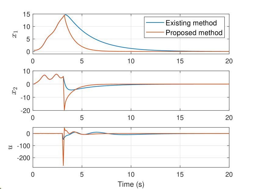
Figure 1: Performance comparison for disturbance level $\delta=0.01$.

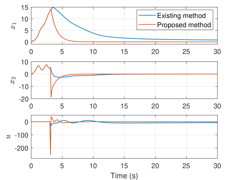
Figure 2: Performance comparison for disturbance level $\delta=0.11$.

The performance of the existing method and the proposed method is compared considered different levels of disturbances (indicated by the value of $\delta$). The existing method [12] is feasible up to $\delta=0.11$. This observation coincides with the findings in [12]. Noticeably, experiments demonstrated that the proposed method remains feasible up to $\delta\approx 0.5$. The comparative results for the disturbance levels $\delta=0.01$ and $\delta=0.11$ are depicted in Fig. 1 and Fig. 2, respectively. It can be seen that the proposed method achieves faster system stabilisation under both levels of disturbances. The obtained controller gain in the existing method is unable to steer the pendulum to the origin $x=(0,0)$ when $\delta=0.11$. Experiments showed that the proposed method can steer the pendulum to the origin up to $\delta\approx 0.5$.

V Conclusion

This paper presents a data-driven SMC to stabilise multi-input multi-output nonlinear systems with partially unknown dynamics and external disturbance. The control design leverages the concept of approximate nonlinearity cancellation, with both the nominal and robust controllers being data-dependent. Compared to the existing data-driven methods, the proposed design is advantageous in terms of achieving robust global stabilisation without requiring that the nonlinearity term goes to zero faster than the state. Simulation results show that compared to the existing method, the proposed design achieves better system stabilisation with robustness to a much higher level of disturbance. Future research will consider data-driven SMC for nonlinear systems with noisy data and applying the proposed design to mixed traffic systems.

References

• [1] C. De Persis and P. Tesi, “Learning controllers for nonlinear systems from data,” Annu. Rev. Control, p. 100915, 2023.
• [2] F. Dörfler, J. Coulson, and I. Markovsky, “Bridging direct and indirect data-driven control formulations via regularizations and relaxations,” IEEE Trans. Autom. Control., vol. 68, no. 2, pp. 883–897, 2022.
• [3] A. Astolfi, “Nonlinear adaptive control,” in Encyclopedia of Systems and Control.   Springer, 2021, pp. 1467–1472.
• [4] M. C. Campi and S. M. Savaresi, “Direct nonlinear control design: The virtual reference feedback tuning (VRFT) approach,” IEEE Trans. Autom. Control., vol. 51, no. 1, pp. 14–27, 2006.
• [5] F. L. Lewis and D. Vrabie, “Reinforcement learning and adaptive dynamic programming for feedback control,” IEEE Circuits Syst. Mag., vol. 9, no. 3, pp. 32–50, 2009.
• [6] C. De Persis and P. Tesi, “Formulas for data-driven control: Stabilization, optimality, and robustness,” IEEE Trans. Autom. Control., vol. 65, no. 3, pp. 909–924, 2020.
• [7] A. S. Bazanella, L. Campestrini, and D. Eckhard, “An introduction to data-driven control, from kernels to behaviors,” in Proc. IEEE Conf. Decis. Control.   IEEE, 2022, pp. 1079–1084.
• [8] W. Tang and P. Daoutidis, “Data-driven control: Overview and perspectives,” in Proc. Am. Control Conf.   IEEE, 2022, pp. 1048–1064.
• [9] T. Martin, T. B. Schön, and F. Allgöwer, “Guarantees for data-driven control of nonlinear systems using semidefinite programming: A survey,” Annu. Rev. Control, p. 100911, 2023.
• [10] M. Guo, C. De Persis, and P. Tesi, “Data-driven stabilization of nonlinear polynomial systems with noisy data,” IEEE Trans. Autom. Control., vol. 67, no. 8, pp. 4210–4217, 2022.
• [11] T. Martin and F. Allgöwer, “Data-driven system analysis of nonlinear systems using polynomial approximation,” IEEE Trans. Autom. Control., DOI: 10.1109/TAC.2023.3321212, 2023.
• [12] C. De Persis, M. Rotulo, and P. Tesi, “Learning controllers from data via approximate nonlinearity cancellation,” IEEE Trans. Automat. Contr., vol. 68, no. 10, pp. 6082–6097, 2023.
• [13] M. Guo, C. De Persis, and P. Tesi, “Data-driven control of input-affine systems via approximate nonlinearity cancellation,” IFAC-PapersOnLine, vol. 56, no. 2, pp. 1357–1362, 2023.
• [14] ——, “Learning control of second-order systems via nonlinearity cancellation,” in Proc. IEEE Conf. Decis. Control.   IEEE, 2023, pp. 3055–3060.
• [15] N. Ebrahimi, S. Ozgoli, and A. Ramezani, “Data-driven sliding mode control: a new approach based on optimization,” Int. J. Control, vol. 93, no. 8, pp. 1980–1988, 2020.
• [16] M. Hou and Y. Wang, “Data-driven adaptive terminal sliding mode control with prescribed performance,” Asian J. Control, vol. 23, no. 2, pp. 774–785, 2021.
• [17] M. L. Corradini, “A robust sliding-mode based data-driven model-free adaptive controller,” IEEE Control Syst. Lett., vol. 6, pp. 421–427, 2021.
• [18] S. Sarpturk, Y. Istefanopulos, and O. Kaynak, “On the stability of discrete-time sliding mode control systems,” IEEE Trans. Autom. Control., vol. 32, no. 10, pp. 930–932, 1987.
• [19] C. Scherer and S. Weiland, “Linear matrix inequalities in control,” Lecture Notes, Dutch Institute for Systems and Control, Delft, The Netherlands, vol. 3, no. 2, 2000.
• [20] J. Löfberg, “YALMIP: A toolbox for modeling and optimization in MATLAB,” in Proc. CACSD, vol. 3, 2004.
• [21] Mosek ApS, “The MOSEK optimization software.” [Online]. Available: https://www.mosek.com