Runtime Monitoring and Fault Detection for Neural Network-Controlled Systems

Abstract

There is an emerging trend in applying deep learning methods to control complex nonlinear systems. This paper considers enhancing the runtime safety of nonlinear systems controlled by neural networks in the presence of disturbance and measurement noise. A robustly stable interval observer is designed to generate sound and precise lower and upper bounds for the neural network, nonlinear function, and system state. The obtained interval is utilised to monitor the real-time system safety and detect faults in the system’s outputs or actuators. An adaptive cruise control vehicular system is simulated to demonstrate effectiveness of the proposed design.

, , ,

1 Introduction

Machine learning techniques including deep neural networks (NNs) are powerful for modelling and controlling complex nonlinear systems such as robots and autonomous vehicles (Moe et al., 2018; Tang et al., 2023). However, NNs are vulnerable to input perturbations such as noise and adversarial attacks. This is even more problematic when NNs are used to generate real-time control actions for automatic systems such as aircraft (Julian and Kochenderfer, 2021), because uncertainties (or deviations) in the NN will be propagated and accumulated the closed-loop, leading to degraded performance and safety concerns (Bensalem et al., 2023). It is thus important to assure real-time safety of NN-controlled systems.

Safety assurance for NN-controlled autonomous systems has been looked at from different angles in the literature. Lots of research has been devoted to formal methods for verifying the robustness of NNs against perturbations (Liu et al., 2021). The formal methods are normally based on interval bound propagation and the solving of optimisation problems such as mixed-integer linear programming (MILP) (Lomuscio and Maganti, 2017), semidefinite programming (SDP) (Lan et al., 2023), and linear programming (LP) (Bunel et al., 2020). However, these works consider NNs as stand-alone components for image classification, natural language processing, etc. Some researchers have considered verifying safety of the NN-controlled systems through reachability analysis. Given an initial state set, they use methods, such as MILP (Karg and Lucia, 2020), SDP (Hu et al., 2020), LP (Everett et al., 2021), or constrained zonotopes (Zhang and Xu, 2022), to compute the reachable set which contains all the possible future system trajectories and check whether this set is within the safe region or not. However, reachability analysis is computationally expensive and has been conducted offline. This method is thus unable to account for system changes due to external disturbances and measurement noise or detect system security issues in a timely manner.

This paper is dedicated to runtime monitoring of NN-controlled autonomous systems to assure their safety. Cofer et al. (2020) propose a rule-based method for monitoring NN-based aircraft taxiing, using a set of monitors to measure the aircraft’s relative position to the runway and NN’s deviation from its training dataset. Xiang (2021) and Wang et al. (2023) develop observers to monitor the state of continuous-time NN-controlled nonlinear systems by taking inspiration from the interval observer technique (Efimov et al., 2013). However, their works do not consider system disturbance or measurement noise, and assume the existence of an interval for the nonlinear function without providing a way to derive it. They adopt the auxiliary network (AN) method to compute the output bounds of NNs, which is applicable to a wide range of activation functions including the most widely used Rectified Linear Unit (ReLU) and tanh (Dubey et al., 2022), but its conservatism results in loose intervals of the system trajectories.

This paper proposes a new interval observer for discrete-time nonlinear systems under disturbance and measurement noise, where the controller is a deep NN with ReLU activations. The proposed observer design is advantageous over the existing methods (Xiang, 2021; Wang et al., 2023) in three aspects: (i) it uses an MILP optimisation approach to obtain the tightest NN bounds, avoiding the conservatism introduced by the AN method. (ii) it provides a systematic way to construct the upper and lower bounds of the nonlinear function; (iii) it ensures that the generated state interval is robust against external disturbance and measurement noise.

2 Problem description and preliminaries

Consider a discrete-time system modelled by

$$x_{t+1} =Ax_{t}+Bu_{t}+Fg(x_{t})+w_{t},$$ (1a)

$$y_{t} =Cx_{t}+v_{t},$$ (1b)

where $t$ is the sampling time. $x_{t}\in\mathbb{R}^{n}$, $u_{t}\in\mathbb{R}^{m}$, $w_{t}\in\mathbb{R}^{n}$, $y_{t}\in\mathbb{R}^{p}$, and $v_{t}\in\mathbb{R}^{p}$ are the vectors of system state, control inputs, external disturbances, measured outputs, and noise, respectively. $g(x_{t})\in\mathbb{R}^{s}$ is the system nonlinearity. $A\in\mathbb{R}^{n\times n}$, $B\in\mathbb{R}^{n\times m}$, $F\in\mathbb{R}^{n\times s}$, and $C\in\mathbb{R}^{p\times n}$ are known constant matrices. In this paper, $u_{t}=f_{\text{nn}}(r_{t},y_{t}^{o})$, where $r_{t}\in\mathbb{R}^{q}$ is the vector of known reference signals and $y_{t}^{o}=C_{o}y_{t}$ which takes partial $y_{t}$ using $C_{o}=[\mathbf{0}_{\ell\times p_{1}}~{}I_{\ell}~{}\mathbf{0}_{\ell\times p-\ell-p_{1}}]$ with the integers $\ell\geq 1$ and $p_{1}\geq 0$. $f_{\text{nn}}\in\mathbb{R}^{m}$ is a $L$-layer feedforward NN given by:

$$z_{0} =[r_{t};y_{t}^{o}],~{}z_{i}=\phi(W_{i}z_{i-1}+b_{i}),~{}i\in[1,L-1],$$

$$f_{\text{nn}}(z_{0}) =W_{L}z_{L-1}+b_{L},$$

where $W_{i}$ and $b_{i}$ are the weight and bias of the $i$-th hidden layer, respectively. $\phi(\cdot)$ is the ReLU activation function with the form $\phi(\hat{z}_{i})=\max(\hat{z}_{i},0)$, where $\hat{z}_{i}=W_{i}z_{i-1}+b_{i}$ and the operation $\max$ is applied elementwise.

This paper aims to design a robustly stable observer that can generate a precise interval for the state trajectory for runtime safety monitoring and detection of actuator or sensor faults.

In this paper, the following notations are defined for a matrix $X$: $X^{+}=\max\{0,X\}$, $X^{-}=X^{+}-X$, and $|X|=X^{+}+X^{-}$. The observer design is based on Assumption 1 and will use Lemma 2.

Assumption 1

The pair $(A,C)$ is observable. $x_{0}\in[\underline{x}_{0},\bar{x}_{0}]$ for some known constant vector $\underline{x}_{0}$ and $\bar{x}_{0}$. $w_{t}\in[\underline{w}_{t},\bar{w}_{t}]$, and $v_{t}\in[\underline{v}_{t},\bar{v}_{t}]$ for all $t\geq 0$, where $\underline{w}_{t}$, $\bar{w}_{t}$, $\underline{v}_{t}$, and $\bar{v}_{t}$ are known bounded signals.

Lemma 2

(Efimov et al., 2013) Given a vector $x\in\mathbb{R}^{n}$ satisfying $x\in[\underline{x},\bar{x}]$ and a constant matrix $X\in\mathbb{R}^{m\times n}$, it holds that $X^{+}\underline{x}-X^{-}\bar{x}\leq Xx\leq X^{+}\bar{x}-X^{-}\underline{x}.$

3 Interval Observer Design

The proposed interval observer needs the intervals for $x_{0}$, $w_{t}$, $v_{t}$, $f_{\text{nn}}(y^{o}_{t},r_{t})$, and $g(x(t))$. The intervals for $x_{0}$, $w_{t}$ and $v_{t}$ are known from Assumption 1, while those for $f_{\text{nn}}(r_{t},y^{o}_{t})$ and $g(x(t))$ are computed below.

Interval of the NN Controller. Let the output $y_{t}^{o}$ satisfy $y_{t}^{o}\in[\underline{y^{o}}_{t},\overline{y^{o}}_{t}]$. It follows from Assumption 1 and Lemma 2 that $\underline{y^{o}}_{t}=C_{o}(C^{+}\underline{x}_{t}-C^{-}\overline{x}_{t}+\underline{v}_{t})$ and $\overline{y^{o}}_{t}=C_{o}(C^{+}\overline{x}_{t}-C^{-}\underline{x}_{t}+\bar{v}_{t}),$ where $[\underline{x}_{t},\overline{x}_{t}]$ is the interval of $x_{t}$ to be generated by the proposed interval observer. Suppose that the NN controller $f_{\text{nn}}(z_{0})$ is bounded as $f_{\text{nn}}(z_{0})\in[\underline{f}_{\text{nn}}(t),\overline{f}_{\text{nn}}(t)]$ for the input region $z_{0}\in[\underline{z}_{0},\overline{z}_{0}]$, where $\underline{z}_{0}=[r_{t};\underline{y^{o}}_{t}]$ and $\overline{z}_{0}=[r_{t};\overline{y^{o}}_{t}]$. Two methods are described below to compute the NN interval $[\underline{f}_{\text{nn}}(t),\overline{f}_{\text{nn}}(t)]$.

The auxiliary network (AN) method described in (Xiang, 2021, Theorem 1) computes the NN interval as follows:

$$\left\{\begin{array}[]{l}\underline{z}_{i}=\phi(\underline{W}_{i}\overline{z}_{i-1}+\overline{W}_{i}\underline{z}_{i-1}+b_{i}),~{}i\in[1,L-1]\\ \underline{f}_{\text{nn}}(t)=\underline{W}_{i}\overline{z}_{i-1}+\overline{W}_{i}\underline{z}_{i-1}+b_{i}\end{array}\right.,$$ (2c)

$$\left\{\begin{array}[]{l}\overline{z}_{i}=\phi(\underline{W}_{i}\underline{z}_{i-1}+\overline{W}_{i}\overline{z}_{i-1}+b_{i}),~{}i\in[1,L-1]\\ \overline{f}_{\text{nn}}(t)=\underline{W}_{i}\underline{z}_{i-1}+\overline{W}_{i}\overline{z}_{i-1}+b_{i}\end{array}\right.,$$ (2f)

where $\overline{W}_{i}=W_{i}^{+}$ and $\underline{W}_{i}=-W_{i}^{-}$. This method ignores the coupling among neurons, resulting in a loose NN interval that will reduce the precision of the state trajectory intervals to be generated by the interval observer.

In this paper, an optimisation method (OP) is proposed to compute a tighter (the best) NN interval by considering the coupling among all neurons. Given the interval of $z_{0}$, the pre-activation bounds $\hat{l}_{i}$ and $\hat{u}_{i}$ of the $i$-th hidden layer, $i\in[1,L-1]$, can be computed using the interval arithmetic method as follows (Liu et al., 2021):

$$\begin{split}l_{0}&=\underline{z}_{0},~{}u_{0}=\overline{z}_{0},\\ \hat{l}_{i}&=\overline{W}l_{i-1}+\underline{W}_{i}u_{i-1}+b_{i},~{}i\in[1,L-1],\\ \hat{u}_{i}&=\underline{W}_{i}l_{i-1}+\overline{W}_{i}u_{i-1}+b_{i},~{}i\in[1,L-1],\\ l_{i}&=\phi(\hat{l}_{i}),~{}u_{i}=\phi(\hat{u}_{i}),~{}i\in[1,L-2].\end{split}$$ (3)

The $j$-th ReLU neuron at the $i$-th hidden layer $z_{i,j}=\phi(W_{i}(j,:)z_{i-1}+b_{i}(j))$ is equivalently represented by the following set of inequalities:

$$\begin{split}&\hat{z}_{i,j}=W_{i}(j,:)z_{i-1}+b_{i}(j),\\ &z_{i,j}\geq\hat{z}_{i,j},~{}z_{i,j}\geq 0,~{}z_{i,j}\leq\sigma_{i,j}\hat{u}_{i,j},\\ &z_{i,j}\leq\hat{z}_{i,j}-(1-\sigma_{i,j})\hat{l}_{i,j},~{}\sigma_{i,j}\in\{0,1\},\end{split}$$ (4)

where $\hat{l}_{i,j}$ and $\hat{u}_{i,j}$ are the lower and upper pre-activation bounds of $\hat{z}_{i,j}$ computed in (3). The binary variable $\sigma_{i,j}$ indicates the status of the neuron: When $\sigma_{i,j}=1$, the neuron is active and the above set of inequalities revert to be $z_{i,j}=\hat{z}_{i,j}$; when $\sigma_{i,j}=0$, the neuron is inactive and the set of inequalities in (4) revert to be $z_{i,j}=0$.

Based on (4), the $j$-th element of the lower bound $\underline{f}_{\text{nn}}(t)$ is solved from the following optimisation problem:

$$\underline{f}^{j}_{\text{nn}}(t):=\underset{\{z_{i}\}_{i=0}^{L-1},\{\delta_{i}\}_{i=1}^{L-1}}{\min}W_{L}(j,:)z_{L-1}+b_{L}(j)$$

$$\text{s.t.}~{}~{}\underline{z}_{0}\leq z_{0}\leq\overline{z}_{0},~{}\hat{z}_{i}=W_{i}z_{i-1}+b_{i},~{}i\in[1,L-1],$$ (5a)

$$z_{i}\geq\hat{z}_{i},~{}z_{i}\geq 0,~{}z_{i}\leq\sigma_{i}\odot\hat{u}_{i},~{}i\in[1,L-1],$$ (5b)

$$z_{i}\leq\hat{z}_{i}-(1-\sigma_{i})\odot\hat{l}_{i},~{}\sigma_{i}\in\{0,1\}^{n_{i}},~{}i\in[1,L-1],$$ (5c)

where $\odot$ is the elementwise product and $n_{i}$ is the number of neurons at the $i$-th hidden layer. The $j$-th element of $\overline{f}_{\text{nn}}(t)$ are solved from an optimisation problem in the same formulation as (5) but with $\min$ being replaced by $\max$. These optimisation problems are MILP problems which can be solved efficiently using off-the-shelf solvers like Gurobi (Gurobi Optimization, LLC, 2023).

By using the computed NN interval $[\underline{f}_{\text{nn}}(t),\overline{f}_{\text{nn}}(t)]$, it follows from Assumption 1 and Lemma 2 that

$$B^{+}\underline{f}_{\text{nn}}(t)-B^{-}\overline{f}_{\text{nn}}(t)\leq Bf_{\text{nn}}(z_{0})$$

$$\leq B^{+}\overline{f}_{\text{nn}}(t)-B^{-}\underline{f}_{\text{nn}}(t).$$ (6)

Interval of the Nonlinear Function. The OVERT method in (Sidrane et al., 2022) is adapted to compute the interval $[\underline{g}(t),\overline{g}(t)]$ for $g(x_{t})$. Its key idea is briefly introduced as below: Let $g_{i}(x_{t})$ be the $i$-th elementary nonlinear function of $g(x_{t})$, where $i\in[1,s]$. Without generality, this paper assumes that $g_{i}(x_{t})$ can be expressed by a conjunction of relations, where each relation is either an elementary function $e(\chi)$ of a scalar variable $\chi$ (e.g., $\sin(\chi)$, $\chi^{2}$, etc) or an algebraic operation (addition $+$ or subtraction $-$). The multiplication ($\times$) and division ($\div$) operations are converted into an exponential of a sum of logarithms, for which the details are referred to (Sidrane et al., 2022, Algorithm 1). Hence, the interval of $g(x_{t})$ can be constructed by stacking the intervals of all elementary functions $g_{i}(x_{t})$, $i\in[1,s]$. Let the scalar variable $\chi$ satisfy $\chi\in[\underline{\chi},\overline{\chi}]$. The interval $[\underline{\chi},\overline{\chi}]$ is divided into $h_{i}+1$ subintervals, where $h_{i}$ is the number of intermediate points between the two endpoints $\underline{\chi}$ and $\overline{\chi}$ to be selected. We then form the upper (or lower) bound by connecting each two neighbouring points using either the secant line (tangent line for lower bound, resp.) if $g_{i}(\chi)$ is convex in that region, or the tangent line (secant line for lower bound, resp.) if $g_{i}(\chi)$ is concave. The obtained bounds are in the form of

$$\overline{g}_{i}(\chi)=\sum_{j=0}^{h_{i}}a_{i,j}\varphi_{i,j}(\chi),~{}\underline{g}_{i}(\chi)=\sum_{j=0}^{h_{i}}b_{i,j}\delta_{i,j}(\chi),$$ (7)

where $\varphi_{i,j}(y_{t}^{o})$ and $\delta_{i,j}(\chi)$ are linear functions, and $a_{i,j}$ and $b_{i,j}$ are constant coefficients. The optimal way of selecting the $h_{i}$ intermediate points is described in Sidrane et al. (2022). A higher value of $h_{i}$ gives a tighter interval but with a more complex expression.

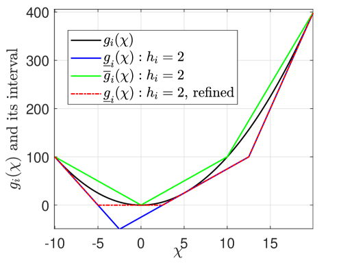
Prior physical knowledge of the nonlinear function $g_{i}(\chi)$ can be used to refine the obtained interval. For example, in the simulation system in Section 5, $g_{i}(\chi)=\chi^{2}$, where $\chi$ is the vehicle velocity. Hence, the lower bound of $g_{i}(\chi)$ satisfies $\underline{g}_{i}\geq 0$ and the lower bound in (7) is refined as $\underline{g}_{i}=\max(\underline{g}_{i},0)$. The refinement can help to obtain a tighter interval, as exemplified in Fig. 1.

Figure 1: Intervals of $g_{i}(\chi)=\chi^{2}$ with and without refinement when $h_{i}=2$ and $\chi\in[-10,20]$.

The interval $[\underline{g}_{i}(x_{t}),\overline{g}_{i}(x_{t})]$ for $g_{i}(x_{t})$ under $x_{t}\in[\underline{x}_{t},\overline{x}_{t}]$ can be derived using (7), as in (Sidrane et al., 2022, Algorithm 2). But this interval depends on $x_{t}$, which is unavailable in the system (1). Instead, the state interval $x_{t}\in[\underline{x}_{t},\overline{x}_{t}]$ will be provided at each time step by the proposed interval observer. This state interval can be used to compute $[\underline{g}_{i}(t),\overline{g}_{i}(t)]$ in real time, as described below:

Given $x_{t}\in[\underline{x}_{t},\overline{x}_{t}]$, the lower bound of $g_{i}(x_{t})$ is redefined as $\underline{g}_{i}(t)$, by solving the following optimisation problem:

$$\underline{g}_{i}(t):=\quad \underset{x_{t},\Omega_{i}}{\min}\quad\Omega_{i}$$

s.t. $$\underline{x}_{t}\leq x_{t}\leq\overline{x}_{t},~{}\underline{g}_{i}(x_{t})\leq\Omega_{i}\leq\overline{g}_{i}(x_{t}).$$ (8)

The upper bound is redefined as $\overline{g}_{i}(t)$ and solved from an optimisation problem with the same form of (3) but with $\min$ being replaced by $\max$.

In some special cases, the nonlinear function $g_{i}(x_{t})$ is monotonic in the region $x_{t}\in[\underline{x}_{t},\overline{x}_{t}]$. One example is the simulation system in Section 5 where $g_{i}(x_{t})=x_{t}^{2}$ and the scalar variable $x_{t}$ is the vehicle velocity satisfying $x_{t}\geq 0$. A graphic view of this example is shown in Fig. 1 by regarding $x_{t}=\chi$ and $\chi\in[0,20]$. In such special cases, solving the optimisation problem (3) is not needed. $\underline{g}_{i}(t)$ and $\overline{g}_{i}(t)$ can be directly computed using

$$\underline{g}_{i}(t)\!=\!\min\{\underline{g}_{i}(\underline{x}_{t}),\overline{g}_{i}(\underline{x}_{t})\},\overline{g}_{i}(t)\!=\!\max\{\underline{g}_{i}(\overline{x}_{t}),~{}\overline{g}_{i}(\overline{x}_{t})\}.\!\!\!\!$$ (9)

By using the computed interval for $g(x_{t})$ and Lemma 2, for $x_{t}\in[\underline{x}_{t},\overline{x}_{t}]$, the interval of $Fg(x_{t})$ is derived as

$$F^{+}\underline{g}(t)-F^{-}\overline{g}(t)\leq Fg(x_{t})\leq F^{+}\overline{g}(t)-F^{-}\underline{g}(t).$$ (10)

Observer Design. For any design matrix $L_{o}\in\mathbb{R}^{n\times p}$, the system (1) can be rewritten as

$$x_{t+1}=A_{o}x_{t}+Bf_{\text{nn}}+Fg(x_{t})+L_{o}y_{t}-L_{o}v_{t}+w_{t}.$$ (11)

where $A_{o}=A-L_{o}C$. Based on Assumption 1, Lemma 2, (3) and (10), the unknown terms $Bf_{\text{nn}}(z_{0})$, $Fg(x_{t})$, $L_{o}v_{t}$, and $w_{t}$ in (11) are replaced with their intervals to formulate the interval observer:

$$\overline{x}_{t+1}={} A_{o}\overline{x}_{t}+B^{+}\overline{f}_{\text{nn}}(t)-B^{-}\underline{f}_{\text{nn}}(t)+F^{+}\overline{g}(t)$$

$$-F^{-}\underline{g}(t)+L_{o}y_{t}-L_{o}^{+}\underline{v}_{t}+L_{o}^{-}\overline{v}_{t}+\overline{w}_{t},$$ (12a)

$$\underline{x}_{t+1}={} A_{o}\underline{x}_{t}+B^{+}\underline{f}_{\text{nn}}(t)-B^{-}\overline{f}_{\text{nn}}(t)+F^{+}\underline{g}(t)$$

$$-F^{-}\overline{g}(t)+L_{o}y_{t}-L_{o}^{+}\overline{v}_{t}+L_{o}^{-}\underline{v}_{t}+\underline{w}_{t}.$$ (12b)

Define the interval width $\delta x_{t}=\overline{x}_{t}-\underline{x}_{t}$. Its dynamics are

$$\delta x_{t+1}=A_{o}\delta x_{t}+D\xi_{t},$$ (13)

where $D=\left[|B|,|F|,|L_{o}|,I\right]$ and $\xi_{t}=[\delta f_{\text{nn}};\delta g(t);\delta v_{t};\delta w_{t}]$ is regarded as the disturbance with $\delta v_{t}=\overline{v}_{t}-\underline{v}_{t}$, $\delta w_{t}=\overline{w}_{t}-\underline{w}_{t}$, $\delta f_{\text{nn}}(t)=\overline{f}_{\text{nn}}(t)-\underline{f}_{\text{nn}}(t)$, and $\delta g(t)=\overline{g}(t)-\underline{g}(t)$.

The gain $L_{o}$ is designed to ensure that the interval observer (12) is sound, i.e., $\overline{x}_{t}\leq x_{t}\leq\underline{x}_{t},\forall t\geq 0$, and the interval width $\delta x_{t}$ is robustly stable against the disturbance $\xi_{t}$.

Theorem 3

For system (1) under Assumption 1, if there is a scalar $\rho$, a diagonal matrix $P$, and matrices $H_{1},H_{2}$ such that the following optimisation problem is feasible:

$$\hskip 51.21504pt\underset{\rho,P,H_{1},H_{2}}{\min}~{}~{}\rho$$

$$\text{s.t.}\hskip 14.22636ptP\succ\mathbf{0},~{}PA-(H_{1}-H_{2})C\geq\mathbf{0},$$ (14a)

$$\hskip 2.84544pt\rho>0,~{}\begin{bmatrix}P-I&\mathbf{0}&[PA-(H_{1}-H_{2})C]^{\top}\\ \star&\rho I&\hat{D}^{\top}\\ \star&\star&P\end{bmatrix}\succ\mathbf{0},$$ (14b)

where $\hat{D}=[P|B|,P|F|,H_{1}+H_{2},P]$, then (12) is a sound interval observer, i.e., $x_{t}\in[\underline{x}_{t},\overline{x}_{t}]$, $\forall t\geq 0$, given that $x_{0}\in[\underline{x}_{0},\overline{x}_{0}]$. Moreover, the interval width $\delta x_{t}$ is robust against the disturbance vector $\xi_{t}$ with the $\mathrm{H}_{\infty}$ performance gain $\sqrt{\rho}$. The observer gain is computed as $L_{o}=L_{o}^{+}-L_{o}^{-}$ with $L_{o}^{+}=P^{-1}H_{1}$ and $L_{o}^{-}=P^{-1}H_{2}$.

Define the errors as $\overline{e}_{t}=\overline{x}_{t}-x_{t}$ and $\underline{e}_{t}=x_{t}-\underline{x}_{t}$. The error dynamics are derived as

$$\overline{e}_{t+1}=A_{o}\overline{e}_{t}+\overline{\Theta}_{t},~{}\underline{e}_{t+1}=A_{o}\underline{e}_{t}+\underline{\Theta}_{t},$$ (15)

where $\overline{\Theta}_{t}=B^{+}(\overline{f}_{\text{nn}}-f_{\text{nn}})+B^{-}(f_{\text{nn}}-\underline{f}_{\text{nn}})+F^{+}(\overline{g}-g)+F^{-}(g-\underline{g})+(\overline{w}_{t}-w_{t})+L_{o}v_{t}-L_{o}^{+}\underline{v}_{t}+L_{o}^{-}\overline{v}_{t}$ and $\underline{\Theta}_{t}=B^{+}(f_{\text{nn}}-\underline{f}_{\text{nn}})+B^{-}(\overline{f}_{\text{nn}}-f_{\text{nn}})+F^{+}(g-\underline{g})+F^{-}(\overline{g}-g)+(w_{t}-\underline{w}_{t})-L_{o}v_{t}+L_{o}^{+}\overline{v}_{t}-L_{o}^{-}\underline{v}_{t}$.

Under Assumption 1, the following inequalities hold:

$$L_{o}v_{t}-L_{o}^{+}\underline{v}_{t}+L_{o}^{-}\overline{v}_{t} =L_{o}^{+}(v_{t}-\underline{v}_{t})+L_{o}^{-}(\overline{v}_{t}-v_{t})\geq\mathbf{0},$$

$$-L_{o}v_{t}+L_{o}^{+}\overline{v}_{t}-L_{o}^{-}\underline{v}_{t} =L_{o}^{-}(v_{t}-\underline{v}_{t})+L_{o}^{+}(\overline{v}_{t}-v_{t})\geq\mathbf{0}.$$

Subsequently, it holds that $\overline{\Theta}_{t}\geq\mathbf{0}$ and $\underline{\Theta}_{t}\geq\mathbf{0}$. Further recalling that $\overline{e}_{0},\underline{e}_{0}\geq\mathbf{0}$ under Assumption 1, it is seen from (15) that $\overline{e}_{t},\underline{e}_{t}\geq\mathbf{0}$, $\forall t\geq 0$, if $A_{o}$ is non-negative (i.e. all its elements are non-negative). Let $P\in\mathbb{R}^{n\times n}\succ\mathbf{0}$ be a diagonal matrix, then $A_{o}$ is non-negative if $PA_{o}\geq\mathbf{0}.$ Submitting $A_{o}=A-(L_{o}^{+}-L_{o}^{-})C$ into the above inequality and introducing $H_{1}=PL_{o}^{+}$ and $H_{2}=PL_{o}^{-}$ yields (14a).

To ensure robust stability of $\delta x_{t}$ against the disturbance $\xi_{t}$, the Lyapunov function $V_{t}=\delta x_{t}^{\top}P\delta x_{t}$ is used. The following relation can be derived from (13):

$$\Delta V_{t}=V_{t+1}-V_{t}={} \zeta_{t}^{\top}\begin{bmatrix}A_{o}^{\top}PA_{o}-P&A_{o}^{\top}PD\\ \star&D^{\top}PD\end{bmatrix}\zeta_{t},$$ (16)

where $\zeta_{t}=[\delta x_{t};\xi_{t}]$ and $D=\left[|B|,|F|,|L_{o}|,I\right]$. Considers the performance index $J=\sum_{t=0}^{\infty}(\delta x_{t}^{\top}\delta x_{t}-\gamma^{2}\xi_{t}^{\top}\xi_{t}+\Delta V_{t})$ for a scalar $\gamma>0$. If $J<0$, the interval width dynamics (13) satisfy the $\mathrm{H}_{\infty}$ performance $\sum_{t=0}^{\infty}\delta x_{t}^{\top}\delta x_{t}\leq\gamma^{2}\sum_{t=0}^{\infty}\xi_{t}^{\top}\xi_{t}$. By using (16), a sufficient condition for $J<0$ is $\delta x_{t}^{\top}\delta x_{t}-\gamma^{2}\xi_{t}^{\top}\xi_{t}+\Delta V_{t}<0$, i.e.,

$$\begin{bmatrix}A_{o}^{\top}PA_{o}-P+I&A_{o}^{\top}PD\\ \star&D^{\top}PD-\gamma^{2}I\end{bmatrix}\prec\mathbf{0}.$$ (17)

Rearranging (17) and applying Schur complement to it, with the introduction of new variables $H_{1}=PL_{o}^{+}$, $H_{2}=PL_{o}^{-}$, and $\rho=\gamma^{2}$, results in the constraint (14b). ∎

4 Runtime Monitoring and Fault Detection

Safety Monitoring. Given the safe state interval $\mathcal{X}_{t}$, it follows from Theorem 3 that the $i$-th state $x_{t}^{i}$ is safe if

$$[\underline{x}_{t}^{i},\overline{x}_{t}^{i}]\subseteq\mathcal{X}_{t}^{i},~{}i\in[1,n].$$ (18)

When this condition is false, safety of $x_{t}^{i}$ is undefined. It could be either $[\underline{x}_{t}^{i},\overline{x}_{t}^{i}]$ is a too coarse outer-approximation of $x_{t}^{i}$ or the state $x_{t}^{i}$ is indeed unsafe. At time $t$, the observer (12) can also provide the one-step ahead predicted state interval $[\underline{x}_{t+1},\overline{x}_{t+1}]$ and output interval $[\underline{y}_{t+1},\overline{y}_{t+1}]$ as follows: $\overline{y}_{t+1}=C^{+}\overline{x}_{t+1}-C^{-}\underline{x}_{t+1}+\overline{v}_{t+1}$, $\underline{y}_{t+1}=C^{+}\underline{x}_{t+1}-C^{-}\overline{x}_{t+1}+\underline{v}_{t+1},$ These one-step ahead predicted intervals can be used to raise alerts of potential unsafe operations in the future. Denote the one-step ahead predicted intervals of $x_{t}$ and $y_{t}$ as $X_{\mathrm{pred},t+1}:=[\underline{x}_{t+1},\overline{x}_{t+1}]$ and $Y_{\mathrm{pred},t+1}:=[\underline{y}_{t+1},\overline{y}_{t+1}]$, respectively. Let the safe intervals of $x_{t+1}$ and $y_{t+1}$ be $\mathcal{X}_{t+1}$ and $\mathcal{Y}_{t+1}$, respectively. At time step $t+1$, the $i$-th state is safe if

$$X_{\mathrm{pred},t+1}^{i}\subseteq\mathcal{X}_{t+1}^{i},~{}i\in[1,n],$$ (19)

and the $j$-th output is safe if

$$Y_{\mathrm{pred},t+1}^{j}\subseteq\mathcal{Y}_{t+1}^{j},~{}j\in[1,p].$$ (20)

When these set inclusions are false, safety of the $i$-th state or $j$-th output is undefined. It could be either that the predicted intervals are too coarse or the real state or output are indeed unsafe. Nevertheless, the information of violation is still practically valuable for alerting unsafe system operations and triggering appropriate preventions.

Fault Detection. Consider the case when an actuator fault $f^{\text{a}}_{t}$ acting on the control signal $u_{t}$ as follows:

$$u_{t}=f_{\text{nn}}(r_{t},y^{o}_{t})+f^{\text{a}}_{t}.$$ (21)

By using the computed interval $[\underline{f}_{\text{nn}}(t),\overline{f}_{\text{nn}}(t)]$, there is a fault in the $i$-th control input channel if

$$u^{i}_{t}\notin[\underline{f}^{i}_{\text{nn}}(t),\overline{f}^{i}_{\text{nn}}(t)],~{}i\in[1,m].$$ (22)

The control input $u_{t}$ is also affected by faults occurring at the output $y^{o}_{t}$ because it is the input to the NN $f_{\text{nn}}$. In the presence of additive faults, the output $y^{o}_{t}$ is represented by

$$y^{o}_{t}=C_{o}(Cx_{t}+F_{\mathrm{s}}f^{\mathrm{s}}_{t}+v_{t}),$$ (23)

with the fault distribution matrix $F_{\mathrm{s}}\in\mathbb{R}^{p\times s}$, where $s\leq p$. This paper focuses on sensor faults, but faults could also be from cyber attacks when some elements of $y^{o}_{t}$ are transmitted through communication networks. Presence of $f^{\mathrm{s}}_{t}$ can also be detected based on the condition (21). But this condition alone does not allow fault isolation because the fault effects due to $f^{\text{a}}_{t}$ and $f^{\mathrm{s}}_{t}$ are coupled.

Due to the nonlinear nature of the NN $f_{\text{nn}}$, it may happen that even a relative large output fault $f^{\mathrm{s}}_{t}$ results in just minor changes to $u_{t}$, making $u_{t}$ remain within the estimated interval and the fault “invisible”. To address this issue, another detecting condition is introduced below: The one-step ahead predicted interval for $y^{o}_{t}$ is $y^{o}_{t+1}\in[\underline{y}^{o}_{t+1},\overline{y}^{o}_{t+1}]$, where $\underline{y}^{o}_{t+1}=C_{o}\underline{y}_{t+1}$ and $\overline{y}^{o}_{t+1}=C_{o}\overline{y}_{t+1}$. At time $t+1$, there is a fault in the $i$-th output $y^{o,i}_{t+1}$ if

$$y^{o,i}_{t}\notin[\underline{y}^{o,i}_{t+1},\overline{y}^{o,i}_{t+1}],~{}i\in[1,\ell].$$ (24)

If (21) is false, but (24) is true, then we are still able to know that there exists faults.

Sufficiency of the checking conditions (18), (19), (20), (22), and (24) relies on tightness of the generated intervals. Tighter intervals increase the capability of safety monitoring and fault detection. The tightness is affected by the priori known intervals for $\omega_{t}$ and $v_{t}$ in Assumption 1 and the intervals for $f_{\text{nn}}$ and $g(x_{t})$ computed in Section 3. Those for $\omega_{t}$ and $v_{t}$ can be improved if a better knowledge of them is available. The proposed OP method has achieved the tightest interval for $f_{\text{nn}}$ with ReLU activations. For the nonlinear function $g(x_{t})$, there may exist other ways to get a tighter interval, which is left for future research.

5 Case Study

Consider an adaptive cruise control (ACC) system:

$$\dot{x}={} A_{c}x+B_{c}u_{\mathrm{e}}+F_{c}g(x)+w,$$ (25a)

$$y={} Cx+v,$$ (25b)

where $x=[p_{\mathrm{l}};v_{\mathrm{l}};a_{\mathrm{l}};p_{\mathrm{e}};v_{\mathrm{e}};a_{\mathrm{e}}]$, $y=[p_{\mathrm{e}};v_{\mathrm{e}};h;\tilde{v}]$, $h=p_{\mathrm{l}}-p_{\mathrm{e}}$, $\tilde{v}=v_{\mathrm{l}}-v_{\mathrm{e}}$, $g(x)=[v_{\mathrm{l}}^{2};v_{\mathrm{e}}^{2}]$, $w=[0;0;2u_{\mathrm{l}};0;0;0]$, and

$$A_{c} =\begin{bmatrix}0&1&0&0&0&0\\ 0&0&1&0&0&0\\ 0&0&-2&0&0&0\\ 0&0&0&0&1&0\\ 0&0&0&0&0&1\\ 0&0&0&0&0&-2\end{bmatrix},B_{c}=\begin{bmatrix}0\\ 0\\ 0\\ 0\\ 0\\ 2\end{bmatrix},F_{c}=\begin{bmatrix}0&0\\ 0&0\\ -\mu&0\\ 0&0\\ 0&0\\ 0&-\mu\end{bmatrix}.$$

The variables $p$, $v$, $a$, and $u$ are the position, velocity, acceleration, and control command of the lead (with subscript $\mathrm{l}$) and ego vehicles (with subscript $\mathrm{e}$), respectively. $\mu$ is the friction parameter. Discretising (25) with sampling time $t_{s}=0.1~{}\mathrm{s}$ gives a system in the form of (1).

Define the safe relative vehicular distance as $d_{\mathrm{safe}}=v_{\mathrm{e}}t_{\mathrm{gap}}+d_{\mathrm{still}}$, where $t_{\mathrm{gap}}$ is the time headway and $d_{\mathrm{still}}$ is the standstill distance. To achieve safe car following, the ACC controller $u_{\text{e}}$ is designed for the ego vehicle to achieve two objectives: When $h\geq d_{\mathrm{safe}}$, $u_{\mathrm{e}}$ takes the speed control mode to maintain the ego vehicle at the driver-set speed $v_{\mathrm{set}}$; When $h<d_{\mathrm{safe}}$, $u_{\mathrm{e}}$ takes the spacing control mode to ensure $h=d_{\mathrm{safe}}$. A 4-layer feedforward NN controller $u_{\text{e}}=f_{\mathrm{nn}}(r,y^{o})$, each hidden layer having 10 ReLU neurons, is trained and implemented, where $r=[v_{\mathrm{set}};t_{\mathrm{gap}}]$ and $y^{o}=[h;\tilde{v};v_{\mathrm{e}}]=C_{o}y$ with $C_{o}=[\mathbf{0}_{3\times 1},I_{3}]$. The simulation parameters are: $\mu\!=\!0.0001$, $t_{\mathrm{gap}}=1.4~{}\mathrm{s}$, $d_{\mathrm{still}}\!=\!10~{}\mathrm{m}$, $v_{\mathrm{set}}\!=\!30~{}\mathrm{m/s}$, $a_{\mathrm{min}}\!=\!-3~{}\mathrm{m/s^{2}}$, $a_{\mathrm{max}}\!=\!2~{}\mathrm{m/s^{2}}$. $v$ is a zero-mean white noise with $|v|\!\leq\!0.001$. The initial state is $x_{0}\!=\![50;20;0;10;20;0]$. The signal bounds in Assumption 1 are set as $\underline{x}_{0}\!=\![49;19;-1;9;19;-1]$, $\overline{x}_{0}\!=\![51;21;1;11;21;1]$, $\underline{v}_{t}\!=\!-0.001$, and $\overline{v}_{t}\!=\!0.001$. Comparison is made for the interval observers using the auxiliary network (AN) or optimisation (OP) methods to compute the interval of $f_{\text{nn}}$. At each time step, the MILP problems are solved using Gurobi and their total computation time is 0.006 s in average. Vehicle reversing is not considered in the simulation, thus each element of the nonlinear function $g(x)=[v_{\mathrm{l}}^{2};v_{\mathrm{e}}^{2}]$ is monotonic and the interval for $g(x)$ is computed using (9).

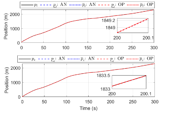
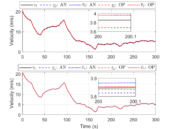
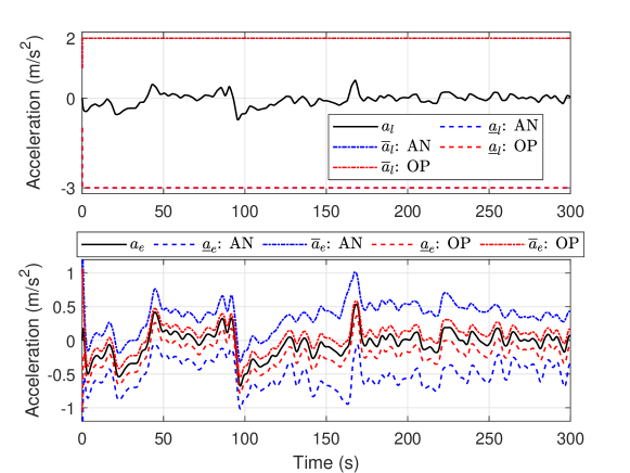
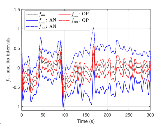
Case 1: The results in Figs. 2 - 5 demonstrate efficacy of the proposed observer in generating sound and robust runtime intervals for the NN controller, vehicle positions, velocities, and accelerations. The results also demonstrate that the intervals based on the OP method are much tighter than those using the AN method, including $f_{\text{nn}}$ in Fig. 2, $v_{\text{e}}$ in Fig. 4, and $a_{\text{e}}$ in Fig. 5. The two methods result in similarly tight intervals for the other vehicle states.

Figure 2: NN controller $u_{\text{e}}=f_{\mathrm{nn}}(r,y^{o})$ and its intervals.

Figure 3: Vehicle positions ($p_{\mathrm{l}}$ and $p_{\mathrm{e}}$) and their intervals.

Figure 4: Vehicle velocities ($v_{\mathrm{l}}$ and $v_{\mathrm{e}}$) and their intervals.

Figure 5: Vehicle accelerations ($a_{\mathrm{l}}$ and $a_{\mathrm{e}}$) and their intervals.

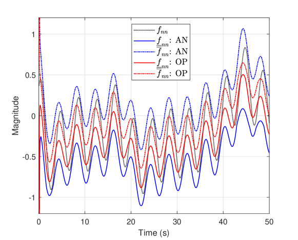
Case 2: Consider the case when there is a bias actuator fault $f_{a}(t)=0.3\sin(0.5\pi t_{s}t),t\geq 0$. Fig. 6 shows that if the interval of $f_{\text{nn}}$ is generated by the OP method, then applying the condition (22) detects the fault. If the interval is generated by the AN method, the fault is not detected. This showcases that the OP method is advantageous over the AN method in actuator fault detection.

Figure 6: Detection of actuator fault $f_{a}(t)=0.3\sin(0.5\pi t_{s}t)$.

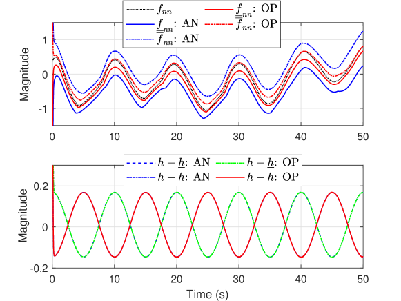
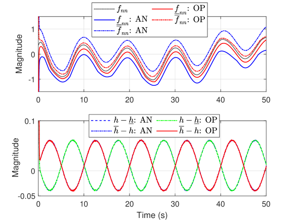
Suppose the lead vehicle sends its real-time position $p_{\mathrm{l}}$ and velocity $v_{\mathrm{l}}$ to the ego vehicle through a wireless communication network. These data are used to construct $y^{o}_{t}$ for generating the NN control law $f_{\text{nn}}$. Consider the case when there is a relative large fault $f_{s}(t)=5\sin(0.2\pi t_{s}t)$ on the data $p_{\text{l}}$ or $f_{s}(t)=\sin(0.2\pi t_{s}t)$ on the data $v_{\text{l}}$. These faults may be due to offsets in the lead vehicle’s sensors (Lan et al., 2020) or cyber attacks in the communication network (Petit and Shladover, 2014). The top subplots in Fig. 7 and Fig. 8 show that using the interval of $f_{\text{nn}}$ from either the AN or OP methods are unable to detect the faults, meaning that the condition (22) alone is not sufficient. The bottom subplots in Fig. 7 and Fig. 8 show that these faults can be effectively detected by both methods using the interval $[\underline{h},\overline{h}]$ of the output $h$ based on the condition (24). If no faults present, the interval observer always generates the interval satisfying $\underline{h}\leq h\leq\overline{h}$, i.e., $h-\underline{h}\geq 0$ and $\overline{h}-h\geq 0$. However, these two inequalities are violated as shown in the bottom subplots in Fig. 7 and Fig. 8, indicating the existence of faults in the system. This confirms the benefits of combining the two conditions (22) and (24), as discussed in Section 4.

Figure 7: Detection of fault $f_{s}(t)=5\sin(0.2\pi t_{s}t)$ on $p_{\text{l}}$.

Figure 8: Detection of fault $f_{s}(t)=\sin(0.2\pi t_{s}t)$ on $v_{\text{l}}$.

6 Conclusions

A robust interval observer is proposed to generate a sound and tight state interval for nonlinear systems controlled by a deep NN. The obtained interval is applied to monitor the runtime system safety and detect faults in the actuators and sensors. Simulation results of the ACC system demonstrate effectiveness of the interval observer and its advantages over the existing design. As for future research, appropriate remedial actions will be proposed to ensure safe operation of NN-controlled systems based on the monitoring and detection results.

References

• Bensalem et al. (2023) Bensalem, S. et al. (2023). What, indeed, is an achievable provable guarantee for learning-enabled safety critical systems. arXiv preprint arXiv:2307.11784.
• Bunel et al. (2020) Bunel, R. et al. (2020). Branch and bound for piecewise linear neural network verification. JMLR, 21(2020).
• Cofer et al. (2020) Cofer, D. et al. (2020). Run-time assurance for learning-enabled systems. In Proc. NFM, 361–368. Springer.
• Dubey et al. (2022) Dubey, S.R., Singh, S.K., and Chaudhuri, B.B. (2022). Activation functions in deep learning: a comprehensive survey and benchmark. Neurocomputing, 503, 92–108.
• Efimov et al. (2013) Efimov, D. et al. (2013). Interval observers for time-varying discrete-time systems. IEEE Trans. Automat. Contr., 58(12), 3218–3224.
• Everett et al. (2021) Everett, M. et al. (2021). Reachability analysis of neural feedback loops. IEEE Access, 9, 163938–163953.
• Gurobi Optimization, LLC (2023) Gurobi Optimization, LLC (2023). Gurobi Optimizer Reference Manual. URL https://www.gurobi.com.
• Hu et al. (2020) Hu, H. et al. (2020). Reach-SDP: Reachability analysis of closed-loop systems with neural network controllers via semidefinite programming. In Proc. CDC, 5929–5934. IEEE.
• Julian and Kochenderfer (2021) Julian, K.D. and Kochenderfer, M.J. (2021). Reachability analysis for neural network aircraft collision avoidance systems. J. Guid. Control Dyn., 44(6), 1132–1142.
• Karg and Lucia (2020) Karg, B. and Lucia, S. (2020). Stability and feasibility of neural network-based controllers via output range analysis. In Proc. CDC, 4947–4954. IEEE.
• Lan et al. (2020) Lan, J., Zhao, D., and Tian, D. (2020). Robust cooperative adaptive cruise control of vehicles on banked and curved roads with sensor bias. In Proc. ACC, 2276–2281. IEEE.
• Lan et al. (2023) Lan, J., Zheng, Y., and Lomuscio, A. (2023). Iteratively enhanced semidefinite relaxations for efficient neural network verification. In Proc. AAAI, volume 37, 14937–14945.
• Liu et al. (2021) Liu, C. et al. (2021). Algorithms for verifying deep neural networks. Found. Trends. Optim., 4(3-4), 244–404.
• Lomuscio and Maganti (2017) Lomuscio, A. and Maganti, L. (2017). An approach to reachability analysis for feed-forward ReLU neural networks. arXiv preprint arXiv:1706.07351.
• Moe et al. (2018) Moe, S., Rustad, A.M., and Hanssen, K.G. (2018). Machine learning in control systems: An overview of the state of the art. In Proc. Innov. Appl. Artif. Intell. Conf., 250–265. Springer.
• Petit and Shladover (2014) Petit, J. and Shladover, S.E. (2014). Potential cyberattacks on automated vehicles. IEEE Trans. Intell. Transp. Syst., 16(2), 546–556.
• Sidrane et al. (2022) Sidrane, C. et al. (2022). OVERT: An algorithm for safety verification of neural network control policies for nonlinear systems. JMLR, 23(1), 5090–5134.
• Tang et al. (2023) Tang, Y. et al. (2023). Perception and navigation in autonomous systems in the era of learning: A survey. IEEE Trans. Neural Netw. Learn. Syst., 34(12), 9604–9624.
• Wang et al. (2023) Wang, T. et al. (2023). Observer-based safety monitoring of nonlinear dynamical systems with neural networks via quadratic constraint approach. Int. J. Control, DOI: 10.1080/00207179.2023.2274924.
• Xiang (2021) Xiang, W. (2021). Runtime safety monitoring of neural-network-enabled dynamical systems. IEEE Trans. Cybern., 52(9), 9587–9596.
• Zhang and Xu (2022) Zhang, Y. and Xu, X. (2022). Safety verification of neural feedback systems based on constrained zonotopes. arXiv preprint arXiv:2204.00903.