A Codesign of Scheduling and Parallelization for Large Model Training
in Heterogeneous Clusters

Abstract

Joint consideration of scheduling and adaptive parallelism offers great opportunities for improving the training efficiency of large models in heterogeneous GPU clusters. However, integrating adaptive parallelism into a cluster scheduler expands the cluster scheduling space. The new space is the product of the original scheduling space and the parallelism exploration space of adaptive parallelism (also a product of pipeline, data, and tensor parallelism). The exponentially enlarged scheduling space and ever-changing optimal parallelism plan from adaptive parallelism together result in the contradiction between low overhead and accurate performance data acquisition for efficient cluster scheduling.

This paper presents Crius, a training system for efficiently scheduling multiple large models with adaptive parallelism in a heterogeneous cluster. Crius proposes a novel scheduling granularity called Cell. It represents a job with deterministic resources and pipeline stages. The exploration space of Cell is shrunk to the product of only data and tensor parallelism, thus exposing the potential for accurate and low-overhead performance estimation. Crius then accurately estimates Cells and efficiently schedules training jobs. When a Cell is selected as a scheduling choice, its represented job runs with the optimal parallelism plan explored. Experimental results show that Crius reduces job completion time by up to ${48.9\%}{}$ and schedules large models with up to ${1.49}{}\times$ cluster throughput improvement on the real testbed.

1 Introduction

Training jobs like pre-training [1, 2, 3, 4] and fine-tuning [5, 6, 7] large models are now vital tasks in both academic and industrial GPU clusters. While training large models requires significant parallel resources, clusters are continually integrating new-generation GPUs to meet the high computational demands. This results in heterogeneity in GPU type, GPU interconnect topology, and so on. To handle the heterogeneity, adaptive parallelism [8, 9, 10] automatically explores the training job’s optimal parallelism on the allocated resources, by combining data, tensor [11], and pipeline parallelisms [12, 13, 14]. Through exhaustive search, adaptive parallelism can always make the best use of the allocated resource.

However, current cluster schedulers [15, 16, 17, 18, 19, 20, 21, 22, 23] do not consider the adaptive parallelism when allocating the heterogeneous resources to the training jobs. We find new opportunities to improve the efficiency of the entire training cluster, if we can jointly consider the scheduling choices and adaptive parallelism. As shown in Figure 1, the scheduler achieves higher cluster throughput by scaling (Case-A) and/or exchanging (Case-B) resources between jobs and running them with adaptive parallelism. The improved efficiency also implies the potential to achieve better scheduling decisions for individual users, i.e., shorter queuing time or job completion time (JCT).

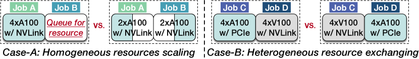
Figure 1: Scheduling decisions contribute to different cluster-level throughput with the same resources: Case-A schedules two jobs onto 4×A100 connected with NVLink, Case-B schedules two jobs onto 4×A100 connected with PCIe and 4×V100 connected with NVLink. Each job runs with the optimal parallelism plan expolored by adaptive parallelism.

In general, a scheduler could make efficient decisions when it has precise performance data for all the scheduling candidates in the entire scheduling space. Following this idea, current efforts on cluster scheduling [19, 20, 22] mainly improve the scheduling efficiency based on extensive performance profiling. They are infeasible to integrate with adaptive parallelism for efficiently utilizing the above opportunities, as the automatic exploration imposes significant overhead when profiling jobs on all possible resources. Specifically, the new scheduling space is a product space of the original one and the parallelism exploration space attributed to adaptive parallelism. The performance data acquisition is hindered by the exponentially enlarged scheduling space. Such full-space profiling requires large distributed resources and time (§2).

Without considering adaptive parallelism, some other scheduling works [21, 24] estimate jobs’ performance across as-yet-unknown resources through simple scaling. While such solutions have low profiling overhead, they are tailored for jobs scaled with only data parallelism. If adaptive parallelism is involved, their estimation cannot maintain high accuracy due to the mismatch between the optimal parallelism plan and the assumed one. Certainly, if we can predict the optimal plan of adaptive parallelism without exploration, the profiling overhead could also be reduced. However, our experiment proves that the prediction accuracy has no guarantee due to the large exploration space (§2.3). Eventually, the low accuracy leads to inefficient scheduling.

This paper therefore presents Crius, a holistic training system that efficiently schedules multiple large models with adaptive parallelism in a heterogeneous cluster. Crius achieves its goal through a novel abstraction named Cell. Crius shards the entire scheduling space across the resource allocation and pipeline parallelism dimensions into Cells, each of which represents a job with designated resource allocation and pipeline stages. When scheduling training jobs, Crius estimates the jobs’ performance with different Cells, and selects the best ones for them. Once a Cell is scheduled, Crius explores its optimal parallelism plan automatically and runs the job. By moving the step of determining the pipeline stages to the scheduling space, the exploration space of finding the optimal parallel plan at runtime for a job shrinks. It exposes the potential for accurate and low-overhead performance estimation.

The key insight of Cell is that the scheduling with adaptive parallelism adheres to a cluster-friendly workflow: each scheduling choice first allocates resources, then determines pipeline stages, and finally partitions each stage independently into coupled data and tensor parallelism combinations. While determining the parallelism before allocating resources seems to be also feasible, it may result in sub-optimal training throughput. This is because there may be a mismatch between the resource requirements of the used parallelism and the resources allocated by the cluster’s optimal scheduling decision. Altering the workflow declines the scheduling efficiency.

To leverage Cell, it is crucial to estimate a Cell’s performance agilely, while there are multiple possible Cells for a job. Crius proposes to profile all communication operators offline, and profile the computation of the model’s pipeline stages independently with data-parallelism-only and tensor-parallelism-only plans at runtime. It is designed based on our observation that the communication part of a job is knowable ahead of scheduling, but the computation part needs to be optimized through compilation techniques [25, 26] after scheduling. The runtime profiling is done on a single GPU with distributed-equivalent compilation, bringing low hardware requirements. Crius then assembles $2^{N_{S}}$ parallelism plans (${N_{S}}$ for pipeline stage number) by combining the 2 profiled parallelism plans of all stages and injecting pre-profiled communication operators between stages. Crius uses the best-performing one among the assembled plans as the Cell’s performance. The plan used for estimation is not the optimal one, but it is representative enough for efficient scheduling, as the parallelism plan assembly is a grid-based sampling across Cell’s entire exploration space.

After a Cell is selected, Crius further explores the optimal parallelism plan. Such exploration could also be time-consuming, as scheduling algorithms may migrate and re-schedule training jobs and the exploration is triggered over and over again in the process. Crius utilizes the assembled plans of a Cell to guide and prune the exploration, as they essentially reflect the Cell’s parallelism favors.

We extensively evaluate Crius with production workloads on both physical and simulative testbeds. Evaluation results show that Crius can achieve ${1.49}{}\times$ higher average cluster throughput, ${71.0\%}{}$ reduction of queuing latency, and ${48.9\%}{}$ reduction of job completion time (JCT) compared to the SOTA training-job schedulers. This paper makes the following contributions.

• We identify the major obstacle in applying adaptive parallelism in existing training clusters is the contradiction between efficient scheduling and low-overhead performance profiling in such a large scheduling space.

• We propose an elegant abstraction, denoted as Cell, serving as an appropriate scheduling candidate, facilitating quick and accurate performance estimation.

• We introduce an innovative estimator capable of accurately estimating the performance of Cell with modest hardware and time overhead, thereby enhancing efficient scheduling.

2 Background and Motivation

2.1 Training with Adaptive Parallelism

Data, tensor [11], and pipeline parallelism [12, 13] are three types of basic parallelism used to train a large model. There are some basic intuitions in manually designing an efficient parallelism plan. For example, when the model’s parameters can fit in a single GPU, data parallelism is preferred. When high-performance inter-GPU communication is enabled (e.g., NVLink [27]), tensor parallelism is preferred. When only poor inter-GPU communication (e.g., network) is available, pipeline parallelism is prioritized.

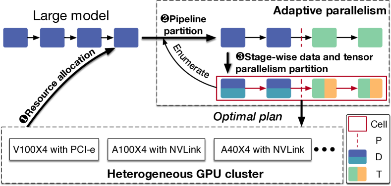
Figure 2: The workflow of training large models with adaptive parallelism in a heterogeneous GPU cluster. D for data parallelism, T for tensor parallelism, P for pipeline parallelism. Cell is the new scheduling candidate proposed by Crius.

Adaptive parallelism [8, 9, 10] enables automatic parallelism optimization without manual design. It achieves the goal by constructing a large space of parallelism plans and exploring it automatically to find the optimal one. Figure 2 shows an example of adaptive parallelism. It enumerates all parallelism plans by running them on corresponding resources to obtain actual performance. The best-performing one among them is then chosen as the final parallelism plan for efficiently training the scheduled large model. Through the above process, adaptive parallelism improves the job’s training efficiency at the cost of hardware resources and tuning time (40 minutes for one exploration in the state-of-the-art system [8]).

2.2 Scheduling Opportunities

With adaptive parallelism, jobs can always make the best use of the allocated resources with enough memory. However, it performs optimally only from the views of individual jobs. If the cluster scheduler could adjust the resources between the training jobs and search the optimal parallelism plans for them, the cluster throughput could be improved. Conjunction consideration of resource scaling and adaptive parallelism greatly enlarge the scheduling space, thus bringing in new scheduling opportunities at the cluster level.

We conduct two experiments to examine the new opportunities. Three large models are involved: WideResnet [28] (WRes in short), BERT [29], and Mixture of Expert [30] (MoE in short). The GPUs are connected via NVLink within the node and Infiniband between nodes. More details are shown in Table 2. Figure 3 depicts the throughput of different choices when scheduling these models with adaptive parallelism. Like many works [31, 19, 32, 15], we use the sum of all training jobs’ throughput as the cluster throughput.

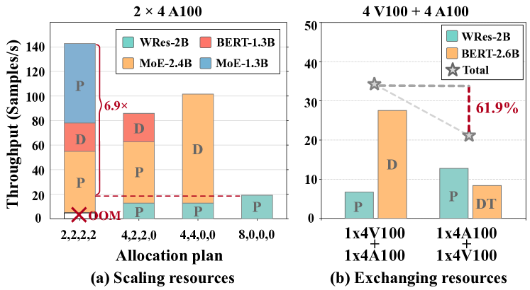
Figure 3: Throughput of different scheduling choices with adaptive parallelism. (a) Homogeneous resources are scaled between models. (b) Heterogeneous resources are exchanged between models. ( Explanation for allocation plan: (4,2,2,0) means 4 GPUs for WRes-2B, 2 GPUs for MoE-2.4B, 2 GPUs for BERT-1.3B and 0 GPUs for MoE-1.3B. OOM indicates that WRes-2B cannot be accommodated with 2xA100 GPUs. D for data parallelism, T for tensor parallelism, P for pipeline parallelism.)

Figure 3(a) shows an example of scaling homogeneous resources between four queuing training jobs. We observe the overall throughput varies significantly across scaling schemes. The main reason is that the jobs using the same resources contribute different throughputs. For example, WRes-2B claims a lot of resources (8GPUs) but contributes little throughput. The cluster scheduler has the opportunity to scale down such models’ GPU numbers, thus allowing more jobs to run and improving the cluster throughput.

We also identify the opportunity to improve cluster throughput by exchanging heterogeneous resources between queuing jobs. For instance, Figure 3(b) presents two available sharing schemes when deploying two models on two types of hardware. As shown in the figure, there is a total throughput gap of $61.9\%$ between the two schemes. This is mainly because when BERT-2.6B is scheduled from the server with 4 A100 GPUs to the one with 4 V100 GPUs, it has to use tensor parallelism due to memory limitations. BERT-2.6B with tensor parallelism suffers from a sharp decline in performance.

Improving the cluster throughput, in turn, has the potential to dramatically optimize the job queuing time, job completion time, and so on. Moreover, when models grow larger and hardware shows more heterogeneity, the exploration space of adaptive parallelism increases. Resource scaling will introduce greater opportunities for the cluster.

2.3 Contradiction in Efficient Scheduling

In §2.2, efficient scheduling decisions are derived based on accurate performance data of each model’s optimal parallelism when running on specific resources. To acquire such data, profiling-based works [23, 15, 22, 20] need to profile each training job on all allocatable resources using adaptive parallelism. However, adaptive parallelism substantially enlarges the scheduling space through numerous job scaling choices and parallelism exploration. Given the tuning overhead in §2, such full-space profiling is unacceptable.

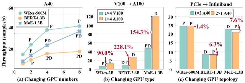
Figure 4: Parallelism plan and job performance variation when changing (a) GPU number: MoE-1.3B scales up linearly, while others approach the performance ceiling; (b) GPU type and (c) GPU topology: models of BERT and MoE have greater variance in throughput due to their change of parallelism plan; (The optimal parallelism plans are marked on top of each bar).

Meanwhile, if the model’s performance can be accurately estimated when running on specific resources with adaptive parallelism, we can also achieve efficient scheduling. However, current estimation-based works [33, 21, 19] only focus on the data-parallelism jobs. Our experimental results in Figure 4 illustrate that the models’ optimal parallelism plans obtained by adaptive parallelism are ever-changing, and the job performance variation is vastly divergent. In this case, simple scaling employed in these works fails to obtain accurate estimation results. And it is challenging to identify a general method for directly predicting the optimal parallelism.

The contradiction between low overhead and accurate performance estimation prevents the efficient scheduling of large models with adaptive parallelism. The above analysis motivates the design of Crius, sharding the scheduling space enlarged by adaptive parallelism into an appropriate granularity as the scheduling candidate. The new scheduling candidate lets the scheduler acquire performance data at a low cost and with high accuracy, thus providing efficient scheduling.

3 Crius Design

The core of Crius is Cell that serves as a new scheduling candidate. Cell defines training jobs’ parallelism exploration space with resources and pipeline stages determined. It guarantees accurate and low-overhead performance data acquisition in a heterogeneous cluster. Cell unifies the cluster scheduling and model parallelization in the following ways: upon scheduling, the cluster scheduler estimates all Cells’ performance and schedules them efficiently; after scheduling, Cell’s parallelism plan is explored automatically.

Figure 5 illustrates the overview of Crius. It currently requires model developers to specify an initial number of GPUs required by the submitted training jobs. Based on this and cluster status, Crius generates multiple Cells for each queuing job as cluster’s scheduling candidates(§6). The pipeline stage of each Cell is determined collaboratively by the specified resource and the job’s model structure (§6.1). As for each Cell, Crius’s agile estimator provides accurate performance estimation. The estimator employs a computation-communication-decoupled method, bringing low temporal and hardware overhead (§5.1). Based on the estimation results, Crius schedules the Cell holistically for different scheduling objectives (§6). Furthermore, to support the joint use of adaptive parallelism and job re-scheduling with negligible overhead, Crius proposes a Cell-limited parallelism tuner. The tuner achieves the goal by pruning the exploration space based on estimation results (§5.2).

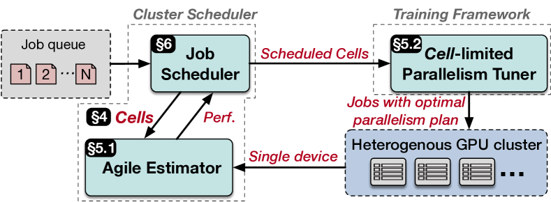
Figure 5: Architecture overview of Crius.

4 Cell as the Core Abstraction

In this section, we first investigate the workflow efficiency of integrating adaptive parallelism in cluster scheduling. Based on the property, we introduce Crius’s core abstraction Cell for sharding the scheduling space.

4.1 Cluster-friendly Scheduling Workflow

In a general scheduler, the scheduling space consists of two dimensions: selecting a scheduled job and allocating resources for it. As illustrated in Figure 6, they are represented on the outer vertical and horizontal axis, respectively. After integrating the adaptive parallelism into cluster scheduling, the new scheduling space is a product space of the original one and the parallelism exploration space, consisting of three dimensions: pipeline, data, and tensor parallelism.

While parallelism exploration enlarges the scheduling space, generating each parallelism plan follows a typical workflow, depicted in the right of Figure 2. Firstly, as parallelism plans partition large models onto allocated GPUs, the parallelism plan generation highly depends on allocated resources. Meanwhile, an implicit priority exists among the three parallelisms incorporated in a parallelism plan. Pipeline parallelism slices the whole model into multiple stages, each of which is a submodel and can be further partitioned independently through data or tensor parallelism [8]. Therefore, pipeline parallelism needs to be prioritized over data and tensor parallelism. Data and tensor parallelism are internal parallelisms of each stage, sharing an equal priority.

When considering adaptive parallelism in the training-cluster scheduler, the above workflow exactly covers the scheduling-decision-making process. Altering the workflow declines the cluster scheduler’s efficiency. E.g., if the pipeline parallelism of a model is determined as 4, the scheduler has to allocate at least 4 GPUs for the model to run properly. This means that the scheduler loses the possibility of scaling the job’s resources to fewer GPUs, which can be the optimal scheduling decision for the cluster. This implies Crius must follow the workflow for cluster-friendly scheduling when integrating adaptive parallelism into cluster scheduling.

4.2 Sharding Scheduling Space into Cells

Figure 6: Example of sharding scheduling space into Cells. Each Cell has determined pipeline stages and allocated hardware. However, tensor and data parallelism are varied in it.

Cell.

With the cluster-friendly workflow in mind, Crius provides an appropriate granularity Cell to shard the scheduling space. As shown in Figure 6, the scheduling space enlarged by adaptive parallelism is sharded into Cells. Each Cell represents a job with determined resource allocation and pipeline stages. Inside the Cell, the data parallelism and tensor parallelism remain to be explored by adaptive parallelism.

With Cells, the cluster scheduler could schedule the training jobs by finding suitable Cells. After a Cell is scheduled, its internal parallelism could be further explored using adaptive parallelism. In this way, not only could Cell have a shrunk exploration space for enabling accurate and low-overhead performance data acquisition, but Crius’s could conduct efficient scheduling using these performance data. Moreover, Crius still follows the cluster-friendly workflow.

Stage determination of a Cell.

As pipeline parallelism is stripped away from parallelism exploration, Crius needs to determine the stages for a Cell at the level of cluster scheduler. To achieve the pipeline’s high efficiency, Crius partitions the model by observing an admitted principle of keeping the computation latency of each stage similar and minimizing the communication between stages. Generally, Crius maps the allocated GPUs to the model’s individual operators according to their floating point operations (FLOPs), then clusters them into stages with minimized communication.

Figure 7 illustrates an example of Crius’s detailed stage partition. Assuming that the partitioned large model has six operators and 8 GPUs are allocated to it, we first map 8 GPUs to each operator based on the ratio of its FLOPs to the entire model. For instance, since $OP_{1}$ accounts for $1/16$ FLOPs of the entire model while $OP_{2}$ accounts for $3/16$, $OP_{1}$ gets 0.5 GPU and $OP_{2}$ gets 1.5 GPU. Meanwhile, the elapsed execution time for each operator can theoretically be calculated as $T_{elapsed}=FLOPs/Number_{GPU}$. This means the execution time of all operators is the same under the above resource allocation scheme. In this way, even if each operator is an independent stage, the operators could construct a full-state pipeline theoretically.

Through the above mapping, Crius can cluster the operators into stages while ensuring the similarity of the execution time of all pipeline stages. Figure 7 shows an example that the operator clustering selects the smallest $3$ inter-operator communication as the clustering boundaries to slice the entire model into 4 pipeline stages. After completion of stage determination, operators’ mapped GPUs are accumulated as the stage’s allocated GPUs. Note that the number of GPUs accumulated for each stage approximates a power of 2. This is the common GPU topology in a training cluster.

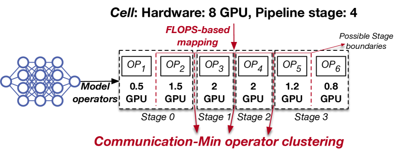
Figure 7: An example of stage determination.

Complexity analysis after sharding.

The Cell abstraction reduces the size of the parallelism exploration space by unbinding the pipeline parallelism from the original adaptive parallelism [8]. For this reason, the scheduling complexity has increased due to the pipeline parallelism. Fortunately, the extended scheduling time is not a big concern in training clusters, as training jobs often take a long time (more than a few hours). We also report the scheduling overhead in §8.7.

5 Mechanisms for Leveraging Cell

Cell unifies cluster scheduler and training framework. At cluster level, the scheduler relies on Cell’s performance estimation for efficient scheduling. At framework level, training jobs need the optimal parallelism plan of the new exploration space defined by Cell to fully utilize the allocated resources. Therefore, in this section, Crius mainly proposes two mechanisms: estimating Cell agilely for scheduler (§5.1) and tuning parallelism under Cell’s limitation for framework (§5.2).

5.1 Agile Cell Estimation

Decoupling communication and computation.

To achieve accurate and agile estimation, we investigate the training of large models. Figure 8 illustrates the example of training a large model using the optimal parallelism plan. The large model consists of 4 pipeline stages running on a total of 8 GPUs, as shown in the figure. Either data or tensor parallelisms further partition each stage onto 2 GPUs to fully utilize the GPU’s high computing power. Communication operators such as send/recv and all_gather connect the stages to form the entire training pipeline.

Obviously, the training execution consists of two categories of operators: computation operators, and communication operators. There is a big difference in optimizing them. As for communication, the optimization algorithm depends on the interconnect between GPUs and nodes. Since the interconnect hardly changes after hardware setup, the latency performance of a communication operator only changes due to the volume of transferred data. As for computation, various compilation optimizations [25, 26] are applied based on specific patterns of computation operators at runtime.

The independence of optimizing computation and communication motivates Crius to decouple the end-to-end performance estimation into two parts: computation parts and communication parts. At offline, Crius can offline obtain distributed-related performance data of communication operators. At runtime, Crius only profiles the computation operators. In this case, we may reduce the overhead of performance data acquisition by accumulating the profiled data of computation and communication operators.

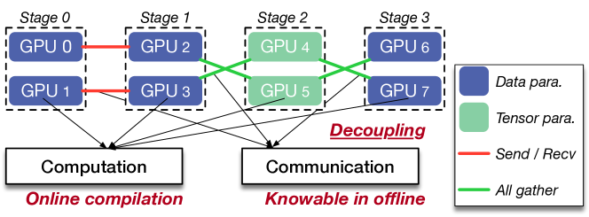
Figure 8: The deployment example of a training job. Computation operators are compiled at runtime, while communication operators are knowable ahead of the job’s submission.

In the light of decoupling, Crius develops an agile Cell estimation method. Although Cell’s pipeline stage is determined, numerous plans remain in its parallelism exploration space. Therefore, the method samples Cell’s exploration space in a grid-based manner and uses the best among the sampled plans as the estimation of Cell. In this way, Crius provides accurate performance data of Cell through representative sampling instead of predicting the optimal plan.

Sampling by parallelism assembly.

Crude sampling could incur a high overhead in terms of time and hardware. As the end-to-end computation can be decoupled, we find that we can assemble the pipeline stages to generate different parallelism plans to reduce the overhead. As shown in Figure 8, send/recv is used to connect stages partitioned by data parallelism, and all_gather is used to connect stages partitioned by tensor parallelism. As for stages partitioned by a hybrid of data and tensor parallelisms, the collaborative usage of send/recv and all_gather is required. This implies that a new parallelism plan can be assembled by changing a stage’s parallelism of a known parallelism plan and the associated communication operators.

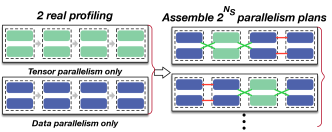
Figure 9: Sampling Cell with parallelism assembly for $2^{N_{s}}$ parallelism plans at the cost of only $2$ physical-device profilings. $N_{s}$ is the stage number.

Therefore, Crius samples the exploration space of Cell using parallelism assembly, as shown in Figure 9. Assuming that Crius has prior knowledge of the performance data of each stage’s computation using the tensor-parallelism-only and data-parallelism-only plans, along with the ability to predict the performance of the associated communication operators, Crius assembles new parallelism plans in the following ways. It combines the two known parallelism plans for each stage and injects communication operators to assemble $2^{N_{S}}$ distinct parallelism plans. The sampling process is clearly gridded and can be conducted at the expense of two physical profiling operations.

Single-device distributed profiling.

To estimate sampled parallelism plans, Crius further presents a single-device distributed profiling to obtain the job’s performance with specified parallelism plan and resource. The profiling is also based on the decoupling observation. We present the workflow of single-device distributed profiling in Figure 10.

When analyzing the specified parallelism plan (data-parallelism-only or tensor-parallelism-only), Crius extracts the computation and communication operators from the training pipeline. Then, Crius performs a distributed-equivalent compilation for computation operators and profiles them. This is totally done on a single GPU. But for communication operators, Crius estimates them through traffic-based interpolation. The data used for interpolation is obtained offline.

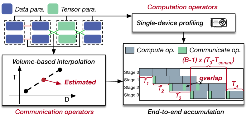
Figure 10: Workflow of single-device distributed profiling ($B$ is the number of microbatches used in the pipeline. Crius follows GPipe [14] to set it to $4\times$ the number of stages).

We adopt a similar method in Alpa [8] to accumulate the computation and communication operators for end-to-end latency. As shown in the lower right of Figure 10, the latency of the entire training pipeline is determined by two parts: (1) the latency of the first micro-batch going through the pipeline ($T_{1}+T_{2}+T_{3}+T_{4}$), (2) the execution time of rest $B-1$ micro-batches dominated by the slowest stage ($(B-1)*(T_{3}-T_{comm.})$). Note that the latency of each stage is the sum of the latency of its computation operators and the latency of the communication operators between it and the previous stage. But when calculating the second part, the communication is overlapped with computation, thus needing to be subtracted.

Based on the above method, Crius could obtain the end-to-end latencies of all assembled parallelism plans. The best among them is taken as the Cell’s estimation. Although this method could not predict the optimal plan directly, the grid-based sampling covers the entire exploration space. The best-performing sampled plan is enough for efficient scheduling.

To avoid the out-of-memory error, Crius also records the memory usage of each stage’s computation operator. If the memory usage exceeds the memory limit of the used GPU, the corresponding parallelism plan is dropped for the stage.

5.2 Cell-guided Parallelism Tuning

When selecting a Cell as the optimal scheduling choice, the corresponding job needs a parallelism plan to best utilize allocated resources. Although the agile estimation is sufficient for efficient scheduling, the parallelism plan selected using estimation may not provide the best performance. This requires Crius to explore the space defined by Cell for the optimal parallelism plan. Unfortunately, the parallelism exploration in previous works [8, 10] needs to enumerate the parallelism plans, which incurs high overhead. Therefore, Crius needs to design a fast parallelism tuning method.

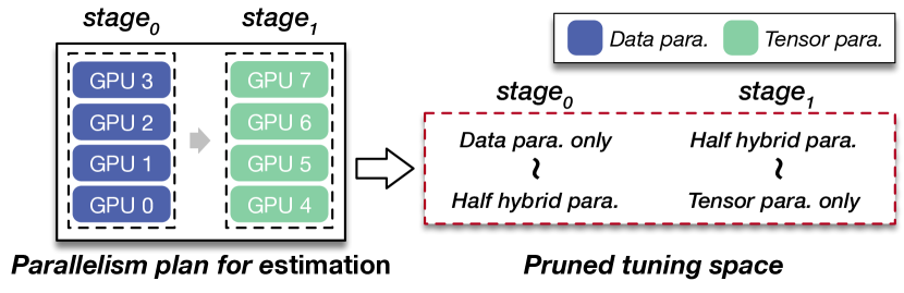
Figure 11: Pruning parallelism exploration space based on estimation results (Assuming that $N$ GPUs are allocated for a single stage, half-hybrid-parallelism refers to first partitioning the stage into $\sqrt{N}$ replicas with data parallelism, then partitioning each replica into $\sqrt{N}$ parts with tensor parallelism).

In Crius, we exploit the estimation results of Cell to guide and accelerate the tuning inside Cell. We notice that Cell’s parallelism plan used for estimation is approaching the optimal one. Hence, Crius prunes the exploration space based on estimation. Figure 11 shows an example of the space pruning. Each stage’s parallelism chosen in the estimated plan is treated as the stage’s parallelism favor. Crius divides the complete exploration space of a single stage into two parts: (data-parallelism-only to half-hybrid-parallelism) and (half-hybrid-parallelism to tensor-parallelism-only). If data parallelism is selected as a stage’s preferred parallelism, the stage will only be tuned within the (data parallelism to half parallelism) range, and the other half will be pruned. The same applies to tensor parallelism.

6 Cluster Scheduling Scheme with Cells

In this section, we introduce how Crius efficiently schedules large models based on the estimation of Cell.

Scheduling in Crius.

Before going into the scheduling details, we would like to emphasize the goals of Crius’s key design. Crius aims to provide accurate performance data for efficient scheduling with adaptive parallelism. Therefore, Crius currently employs a simple heuristic algorithm to greedily schedule the large-model training jobs with resource scaling. Techniques based on solvers [21, 20, 33] could also be applied to enhance Crius, which are orthogonal to Crius’s primary focus. Moreover, while Crius aims to maximize the cluster throughput in this section, Crius is easy to adapt to other scheduling objectives. In §8.5, we extend Crius to support deadline-aware objectives and discuss its performance with a comprehensive evaluation.

6.1 Scheduling Policy

1:cells_set: all scheduling candidates of running jobs

2:function SchedArrival(new_jobs)

3:    for $job\in new\_jobs$ do

4:         $//$ Initalize Cells for job and update them to $cells\_set$

5:         $cells\_set.update(cells_{job})$

6:         $feasible\leftarrow$ CellBasedSched($job$)

7:         if $\text{{not} }feasible$ then Pend($job$)              

8:    FinalizeAlloc($run\_jobs$)

9:function SchedDeparture()

10:    for $job\in pend\_jobs$ do CellBasedSched($job$)     

11:    $//$ Extra scheduling for utilizing released resource

12:    CellBasedSched()

13:    FinalizeAlloc($run\_jobs$)

14:function CellBasedSched($job=None$)

15:    $//$ Explore candidate scheduling plans

16:    $choices\leftarrow$ScaleResource($run\_jobs,cells\_set,job$)

17:    $//$ Select based on cell estimation

18:    $best\_choice\leftarrow$ BestPerf($choices,cells$)

19:    $feasible\leftarrow$VritualAlloc($run\_jobs,best\_choice,job$)

20:    return $feasible$

Algorithm 1 Cell-based Job Scheduling

Policy.

Algorithm 1 shows the pseudocode of Crius scheduling. Basically, the algorithm is triggered when a new job arrives (lines 2-8) or a job completes (lines 9-13). When a new job arrives, the algorithm initializes Cells (line 4) and schedules it based on Cells (line 6). Specifically, the scheduling algorithm (lines 14-20) explores potential scheduling choices with resource scaling. With the performance estimation of Cells, the algorithm selects the best choices (e.g., maximum cluster throughput) and reschedule all jobs. If no feasible scheduling choice is found, the job is pending. When running jobs are complete, the algorithm first attempts to resume the pending jobs. If there are no pending jobs, the algorithm triggers extra scheduling to allocate released resources to running jobs (line 11). Note that in each Cell-based scheduling, the best plan is applied virtually on running jobs. The real job scheduling only happens at the end (lines 8&13).

Initializing Cells.

As for new coming jobs, Crius needs to initialize Cells for them. Crius now requires the user to specify an initial GPU number $N_{G}$ for the submitted job. Based on the GPU number, Crius selects 3 available values ($N_{G}/2,N_{G},2N_{G}$) to generate the Cells. As for the pipeline stage number, Crius allows $\log N_{G}$ choices ranging from $1$ to $N_{G}$. Because Crius requires a single device to profile the job on each kind of GPU, profilings on heterogeneous GPUs are done in parallel. Therefore, the total time complexity for generating Cells for a new job is $O(3*\log N_{G})$. We evaluate the overall profiling overhead in §8.2.

Scaling training jobs.

When scheduling new jobs, Crius explores scheduling choices with resource scaling. This exploration tries to scale the GPU types and numbers of both running jobs and new-coming jobs. When cluster resources are insufficient, Crius selects jobs to downscale their used GPU numbers or moves them to another type of GPU with sufficient resources. When idle resources exist, Crius performs the reverse scaling. The scaling principle is searching all scheduling choices under the constraint of cluster resources. Specifically, the sum of all Cell’s resources in a scheduling choice should not exceed the cluster resource limit. To avoid scheduling overhead, Crius uses a hyperparameter called search depth, which is the maximum job scaling times for generating a scheduling choice in Algorithm 1 line 18. We evaluate the impact of search depth in terms of overhead and scheduling efficiency in §8.7.

Opportunistic execution.

To avoid the starvation of models that require many GPUs, Crius employs opportunistic execution. When the idle resources are insufficient for a queuing job, Crius pends it and opportunistically launches other jobs to utilize the idle resources. Once the minimum resource requirement for the pending job is satisfied, the opportunistic jobs will be suspended to launch the pending one.

7 Implementation

We implement Crius with 10,900 LoC of Python: 5,400 lines for the scheduler and 5,100 lines for the Cell’s agile estimator, and 400 lines for Cell-guided parallelism tuner, and only 400 lines for Crius’s simulator. Crius’s simulator shares most of the scheduling logic with the scheduler for the physical testbed, thus providing high fidelity. Specifically, we use gRPC to communicate between the scheduler and distributed workers. At runtime, Crius schedules jobs with the interval of 5 minutes and inspects the runtime status of training jobs every 20 seconds.

We implement Crius’s parallelism tuner based on Alpa [8]. In this case, Crius’s estimator is built on Jax [34] and XLA [35], which is also the backend of Alpa. Crius simulates the distributed training on a single device to obtain the distributed-equivalent compilation for all pipeline stages. Moreover, the estimator has a C++ backend with about 500 LoC, enabling Crius to capture the latency of computation operators with Nvidia CUPTI [36]. Based on these techniques, Crius’s estimator obtains accurate latency of computation operators with low overhead. As for communication operators, offline profiling is implemented based on XLA [35], NCCL [37], and Ray [38] for all used GPUs.

8 Evaluation

In this section, we evaluate the effectiveness of Crius on a heterogeneous physical cluster and a simulated large-scale cluster with three production traces.

8.1 Experimental Setup

Physical testbed.

We evaluate Crius on a heterogeneous cluster of 32 servers and 64 GPUs. Specifically, 16 servers are equipped with Intel Xeon Gold 5318Y CPUs (256 GB memory) and 2 Nvidia A40 GPUs (48 GB memory). The other 16 servers are equipped with the same CPUs but 2 Nvidia A10 GPUs (24 GB memory). Servers with A40 GPUs are interconnected using Nvidia Mellanox Infiniband ConnectX-5 [39], while A10 GPU servers are interconnected using Nvidia Mellanox Infiniband ConnectX-6 [40].

Table 1: Machine specs of simulated heterogeneous GPU cluster. GPUs with ^† are equipped with NVLink [27] connection.

GPU Type	Arch	Mem(GiB)	Connect.	#Nodes	#GPUs
A100†	Ampere [41]	40	Mellanox CX5 [39]	80	4
A40	Ampere	48	Mellanox CX5	160	2
A10	Ampere	24	Mellanox CX6 [40]	160	2
V100†	Volta [42]	32	Mellanox CX5	20	16

Simulated cluster with higher heterogeneity.

The simulated cluster has 1,280 GPUs of four types: A100, A40, A10 with Ampere architecture and V100 with Volta architecture. Detailed specifications are listed in Table 1.

Table 2: Model configurations used in the experiments.

Model	Global Batch Size	#Params (billion)
Wide-ResNet [43]	[256, 512, 1024]	[0.5, 1.0, 2.0, 4.0, 6.8]
BERT [44]	[128, 256, 512]	[0.76, 1.3, 2.6, 6.7]
GShard MoE [45]	[256, 512, 1024]	[0.69, 1.3, 2.4, 10, 27]

Workloads.

We use three large-scale models in Table 2 as the workloads. The selected models are the same with state-of-the-art work [8]. We use two-week traces of 13,000+ jobs from the production Philly trace [46]. Furthermore, we also use Helios Venus trace [47] and Alibaba PAI trace [48] to evaluate Crius. While each job record consists of job id, submission time and duration, we randomly generate the GPU amount and GPU type to adapt traces to heterogeneous scenarios. The number of iterations in Philly trace is calculated from scaling by global batch size. In the other two traces, we randomly generate iteration amounts based on trace workload.

Baselines.

We compare Crius with four baselines:

First-Come-First-Served (FCFS): FCFS is widely applied in cluster schedulers (e.g., Kubernetes [49], Yarn [50]).

Gandiva: Gandiva [15] utilizes domain-specific knowledge to introspectively refine scheduling decisions based on runtime profiling. While it could adjust the GPU quota and topology, it ignores the GPU heterogeneity.

Gavel: Gavel [20] is a heterogeneity-aware scheduler designed for various scheduling policies, including throughput maximization. Although it considers the GPU heterogeneity, it does not support the scaling of GPU numbers.

ElasticFlow: ElasticFlow [19] is an adaptivity-aware scheduler with elastic scaling of distributed DL jobs in a homogeneous cluster. It provides a deadline-aware policy and a throughput-oriented policy.

It should be noted that Crius is the first work to support the joint use of resource scaling and adaptive parallelism. For a fair comparison, we enable Alpa’s adaptive parallelism in the baselines’ job training process but only allow them to schedule jobs with data profiled from data parallelism.

8.2 Efficiency of Crius Abstraction

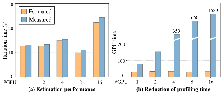
Figure 12: The estimation accuracy and GPU time reduction of Cell abstraction. Estimated denotes conducting Crius’s single-device distributed profiling. Measured denotes directly measuring performance. We increase the model size as the number of GPUs increases.

We evaluate the Cell estimator and the parallelism tuner with a focus on two key aspects: the accuracy of performance estimation and parallelism tuning, and the efficiency of overhead reduction. As for the generated parallelism inside the Cell, we define estimation accuracy as $1-(T_{e}-T_{d})/T_{d}$, where $T_{e}$ and $T_{d}$ are the iteration time obtained from estimation and direct profiling, respectively. As for the scheduled job, we define tuning accuracy as $1-(T_{c}-T_{o})/T_{o}$, where $T_{c}$ and $T_{n}$ are the iteration time of the optimal parallelism searched by Crius and full-space profiling, respectively.

Evaluate Cell estimation.

Figure 12(a) shows the accuracy of the agile Cell estimator. We observe that Crius achieves the estimation accuracy of $93.4\%$ on average and $90.5\%$ at worst. This is because Crius finely models the training pipeline with the accurate overhead of decoupled computation and communication operators obtained from profiling.

Figure 12(b) presents the profiling time reduction of the agile Cell estimator compared to profiling a real job. We use GPU time as the evaluating metric [32], and evaluate our estimator on various configurations (changing model, parallelism and hardware). As shown in the figure, Crius improves the profiling efficiency by $18.1\times$ on average, and $2.55\times$ at least. This comes from two reasons: (1) The profiler eliminates redundant execution of the same partitions within one stage and profiles only the minimal computation operators on one device; (2) Intra and inter-stage communication operators are not online profiled, which could be time-consuming with intensive communication traffic or poor bandwidth.

In Crius’s scheduling workflow, cells of each job are initialized with the time complexity of $O(3*\log N_{G})$ (as discussed in §6.1). With Crius’s distributed profiler, the average profiling time for one parallelism is reduced to about $30$ seconds. As Crius samples 2 parallelisms in one Cell (as discussed in §5.1), the average profiling time for one Cell on only one GPU is about 1 minute. Based on this, Crius guarantees that the profiling time of one job does not exceed 30 minutes, which is comparable to previous works [19, 22].

Evaluate Cell-guided tuning.

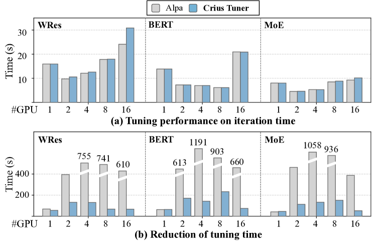
Figure 13: Tuning time reduction and tuning performance with Cell-based estimation and pruning. Unpruned denotes directly searching optimal parallelism. We increase the model size as the number of GPUs increases.

Figure 13(a) shows the tuning accuracy of Cell. We observe that Cell-guided tuning achieves the tuning accuracy of $96.2\%$ on average, as for the throughput of the searched optimal parallelism. This is because the estimator performs grid-based sampling within the entire scheduling space, and therefore can generate a coarse-grained performance surface. Based on that, Crius locates the possible positions of the optimal parallelism and shards the parallelism searching space nicely.

Figure 13(b) shows the reduction of tuning time by searching with Cell estimation. It is observed that Cell-guided tuning improves the profiling efficiency by $5.48\times$ on average and $10.88\times$ at most. This comes from the accurate Cell estimation and Cell-guided tuning. With Cell estimation enabled, the tuner searches only a small subset of candidate parallelisms with ignorable accuracy loss instead of performing full-space enumerating for the optimal parallelism.

8.3 Evaluation on a Real Testbed

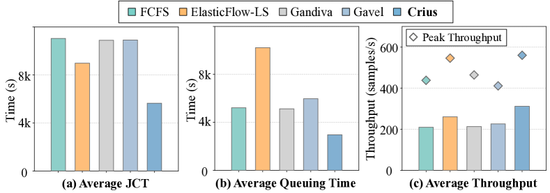
Figure 14: Performance analysis of Crius and baselines on physical testbed with 64 GPUs. ElasticFlow-LS denotes the primary ElasticFlow policy with loosened job deadline [19].

We evaluate the performance of Crius on a heterogeneous physical testbed with 32 A40 GPUs and 32 A10 GPUs, using a 6-hour trace of 244 jobs from Microsoft Philly trace [46].

Performance analysis.

Figure 14 presents the comprehensive performance of Crius. From the job perspective, Figure 14(a) and Figure 14(b) show the average job completion time (JCT) and queuing time of all jobs. We observe that Crius reduces the average JCT by up to $48.9\%$ and the average job queuing time by up to $71.0\%$. This comes from two reasons. On the one hand, Crius efficiently locates the near-optimal parallelism. On the other hand, Crius performs elastic scheduling on training jobs, bringing better resource utilization and more execution opportunities.

From the cluster perspective, Figure 14(c) evaluates the performance of the cluster-wide throughput of Crius. We observe that Crius outperforms other systems with up to $1.49\times$ higher average throughput and $1.36\times$ higher peak throughput. This also comes from the efficient scheduling based on accurate Cell’s performance estimation.

It should be noted that ElasticFlow with loosened job deadline (ElasticFlow-LS) performs best among baselines in terms of average JCT and cluster throughput. This is because it scales down small jobs when the workload is high to accommodate more jobs and maximize throughput. However, since ElasticFlow-LS schedules with the profiled throughput of data parallelism, it always overestimates the minimum required share of large jobs with adaptive parallelism enabled (in most cases, data parallelism consumes more GPU memory). Therefore, the average JCT is lower than other baselines (admitted jobs are allocated with more GPUs), but the job queuing time remains poor performance (more large models are pending).

Simulation fidelity.

To evaluate the fidelity of the simulation, we further conduct simulations with the same experimental configurations. The average simulation error of Crius and other baselines in estimating cluster throughput is $3.16\%$, while $7.31\%$ in estimating JCT. This confirms the high fidelity of our upcoming large-scale simulations.

8.4 Large-Scale Simulations

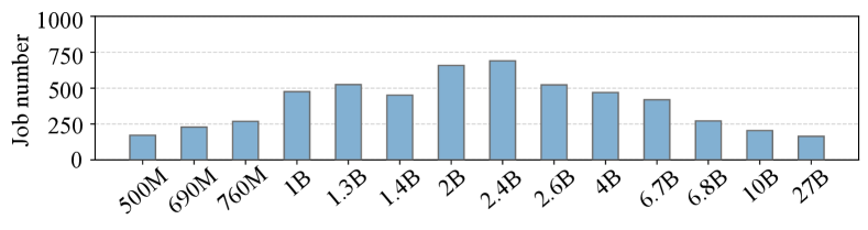
Figure 15: Distribution of model size used in the workload of large-scale simulations.

We further evaluate Crius on a much larger heterogeneous simulated cluster with 1,280 GPUs and four GPU types. The cluster specifications are listed in Table 1. The distribution of the model size is illustrated in Figure 15.

Overall performance.

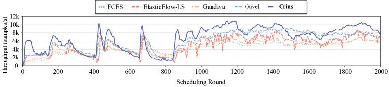
Figure 16: Cluster throughput of the large-scale simulation in one-week Philly trace with heavy workloads. The time interval for each scheduling round is set to five minutes.

Figure 16 presents the overall analysis on the cluster throughput of Crius and all baselines. We observe that Crius performs much better on scaling up with burst workload than other baselines (e.g., range 850-1200). Besides, Crius scales down earlier than other baselines when the cluster workloads decrease (e.g., range 700-800). This indicates that jobs are efficiently completed in Crius, leading to better JCT performance.

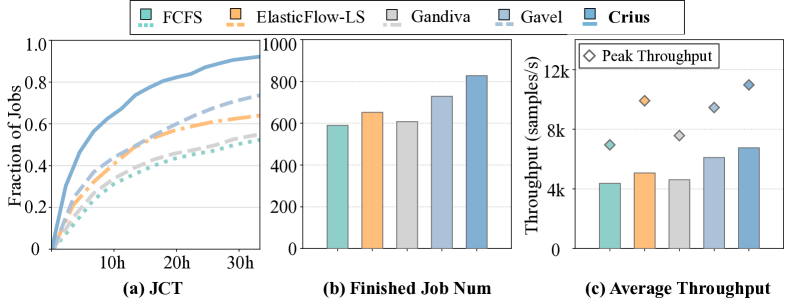
Figure 17: Performance analysis of Crius and baselines on large-scale simulated testbed.

Figure 17 further provides numerical comparisons of Crius with other baselines. As illustrated in Figure 17(a), we observe that Crius provides much lower average JCT than other baselines by $81.3\%$ (FCFS), $75.8\%$ (ElasticFlow-LS), $80.1\%$ (Gandiva) and $66.4\%$ (Gavel). With such a significantly lower average JCT, Crius also completes up to $1.29\times$ more jobs than other baselines, as illustrated in Figure 17(b).

Figure 17(c) further presents the performance comparisons from the cluster perspective. We observe that Crius outperforms the other baselines, achieving up to $1.54\times$ higher average throughput and $1.57\times$ higher peak throughput. However, we also observe that there is a only $10.7\%$ gap of peak throughput between Crius and ElasticFlow-LS. This is because ElasticFlow-LS is also capable of scaling up and increasing cluster throughput when sufficient jobs are submitted for all types of GPUs. However, this is rare across the trace. Therefore, the gap in average throughput between ElasticFlow-LS and Crius is larger than the peak one.

Furthermore, the average number of job restarts in Crius is only $2.29$. This is because Crius’s scheduling choice is based on accurate estimation, and the scheduler limits the search depth for scaling training jobs to avoid frequent rescheduling. In our simulation, we set the search depth to $3$. Further evaluation of this hyperparameter is given in §8.7.

Evaluate with other traces.

We select another two traces (Helios Venus [47], PAI [48]) to further evaluate the performance of Crius. We choose a one-day trace with moderate workloads from Helios Venus and a one-day trace with low workloads from PAI. Crius consistently outperforms other baselines. In Figure 18(a) and Figure 18(b), we observe that Crius surpasses other baselines on the average JCT with a $64.7\%$ reduction with moderate workloads and a $66.3\%$ reduction with low workloads. This advantage also appears in both traces’ maximum and median JCT. Figure 18(c) and Figure 18(d) present the throughput performance with two traces. Crius achieves up to $1.48\times$ (for Helios Venus) and $1.29\times$ (for PAI) higher average throughput and $1.92\times$ (for Helios Venus) and $2.63\times$ (for PAI) higher peak throughput.

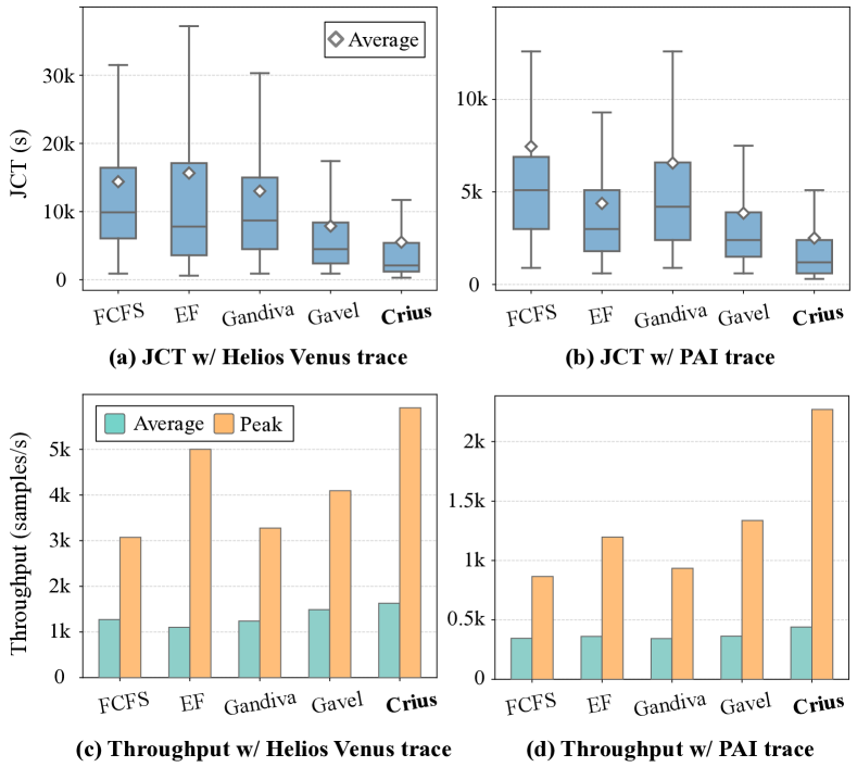
Figure 18: JCT and throughput performance of Helios Venus trace with moderate workloads and PAI trace with low workloads. EF denotes the ElasticFlow-LS policy. Other experiment settings are the same as Figure 16.

8.5 Generality of Crius

To demonstrate the generality of Crius, we follow [19] to extend Crius to support deadline-aware scheduling. Specifically, when making scheduling decisions, Crius provides strict deadline guarantees for each scheduled job while optimizing cluster-wide performance. Crius early drops those jobs that cannot be completed before their deadlines.

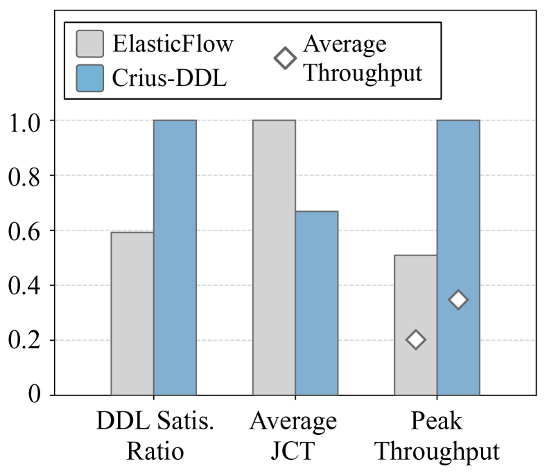
Figure 19: Performance of Crius with deadline-aware, in terms of normalized deadline satisfactory ratio, JCT, and throughput.

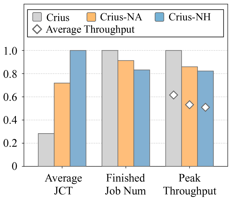
Figure 20: Ablation study of Crius on adaptivity and heterogeneity, in terms of normalized JCT, the number of finished jobs, and throughput.

Figure 20 illustrates the performance analysis of deadline-aware Crius (Crius-DDL). In addition to JCT and throughput, we further evaluate Crius-DDL with the metric deadline satisfactory ratio defined in ElasticFlow [19], which is the ratio of jobs that can satisfy their deadline requirement among all training jobs. We observe that Crius-DDL surpasses ElasticFlow with a $1.69\times$ improvement in deadline satisfactory ratio and a $33.1\%$ reduction in JCT. Besides, Crius-DDL achieves a $1.72\times$ higher average throughput and $1.96\times$ higher peak throughput than ElasticFlow. This comes from the more efficient scheduling choices based on the accurate performance estimation of Cells. Since Crius utilizes cluster resources better, more jobs can be admitted while satisfying their deadline requirements.

8.6 Attributes of Crius’s Benefits

We evaluate the benefits of different types of resource scaling from the view of cluster and individual jobs. We follow Sia [21] to define adaptivity scaling as changing the allocated number of GPUs, and heterogeneity scaling as changing the allocated GPU type.

Figure 20 presents the ablation results. Without adaptivity scaling (Crius-NA, Crius gets a $2.54\times$ higher average JCT and an $8.69\%$ reduction in the number of finished jobs. From the cluster perspective, Crius suffers a $13.6\%$ reduction in the average throughput and a $14.1\%$ reduction in the peak throughput. When disabling heterogeneity scaling (Crius-NH, the average JCT is $3.53\times$ higher. In this case, only $83.2\%$ of the training jobs are completed compared to the oracle of Crius. Besides, the average throughput is reduced by $17.3\%$ and the peak throughput is reduced by $17.7\%$.

We also observe that the overall performance of Crius-NA outperforms Crius-NH. This is due to the high heterogeneity of the simulated testbed. It is also the reason why Gavel (heterogeneity-aware) outperforms ElasticFlow (adaptivity-aware) on the simulated testbed but does worse on the physical testbed. After all, there are 4 kinds of GPUs in the simulated testbed but only 2 kinds of GPU in the physical testbed.

8.7 Impact of search depth

We evaluate the impact of search depth on both scheduling overhead and scheduling efficiency. To better illustrate the performance gaps, we increase the density of job submissions to simulate extremely heavy workloads.

Scheduling overhead.

Figure 21(a) shows the scheduling overhead of one job with various values of search depth. We observe that as the search depth increases, the scheduling overhead for one job increases from $0.88$ to $5.98$ seconds. Compared to the long-term training periods of large-model jobs, the scheduling overhead can be ignored with the limited average job rescheduling times (§8.4).

Scheduling efficiency.

Figure 21(b) and (c) show the performance gaps in the average JCT and the cluster-wide throughput with varied search depths. As the depth increases, we observe that the scheduler reduces the average JCT by $14.6\%$ and achieves $1.03\%$ higher average throughput.

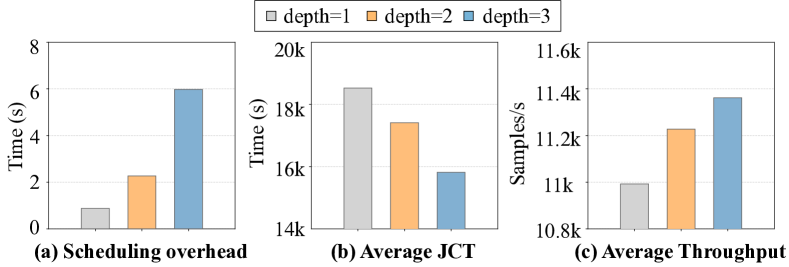
Figure 21: Evaluating scheduling efficiency and overhead with different search depths.

9 Related Work

Deep learning cluster scheduler.

Research on tailored schedulers for DL training jobs has surged in recent years [21, 51, 15, 17, 52, 53, 22, 54, 55, 32, 56].

Some efforts [15, 19] aim to improve the system throughput with scaling of GPU numbers. Gandiva [15] profiles jobs and schedules them with migration and other mechanisms. ElasticFlow [19] enables deadline-aware scheduling for jobs. These works rely on job profiling to conduct efficient scheduling choices. They perform well for small and data-parallelism-only jobs, which can be profiled with low overhead. They are incompatible with large models running with adaptive parallelism, which enlarges the scheduling space for profiling.

Several research works [20, 56] focus on the heterogeneous cluster, which exposes scheduling opportunities for high throughput. Gavel [20] provides customized scheduling policies for jobs heterogeneously. Gandiva_fair [56] considers the fairness of different training jobs leveraging the heterogeneity of GPUs. These works fail to scale the used GPUs, and also rely on profiling for efficient scheduling.

Some prior works [33, 21] exploit the adjustment of DL jobs’ attributes during the scheduling. Pollux [33] dynamically changes the used GPU numbers, batch size, and learning rate of jobs to maximize goodput. Sia [21] further introduces heterogeneity-awareness. However, these works estimate and schedule resource-adaptive jobs, assuming only data parallelism is used for scaling, thus incurring inefficient scheduling for jobs with adaptive parallelism. In Crius, we do not change training jobs’ hyperparameters that affect the model accuracy. Thus, we do not compare Crius with these works.

Performance modeling of training jobs.

There are some previous works [57, 58, 59, 60, 61] on modeling the end-to-end performance of training jobs. Habitat [57] performs runtime prediction on the computation performance of small models for one GPU. Daydream [58] explores the efficacy of DNN optimizations in distributed training. DPRO [59] collects runtime traces and analyzes performance bottlenecks. FasterMoE [61] analytically models communication and computation in distributed training of MoE. These works target models running either on a single GPU or with a static parallelism plan. Hence, they can not provide the accurate estimation for Crius.

10 Conclusion

In this paper, we identify new opportunities brought by joint optimization of cluster scheduling and adaptive parallelism. We propose Crius, a holistic training system for scheduling large models with adaptive parallelism on heterogeneous GPU clusters. The core of Crius is Cell, a new scheduling candidate exposes the potential for accurate performance estimation with low overhead. By leveraging Cell, Crius efficiently schedules training jobs with adaptive parallelism. The scheduled jobs run with the optimal plan searched in the parallelism exploration space defined by Cell. The evaluation shows that Crius schedules large models with up to ${1.49}{}\times$ cluster throughput improvement and reduces JCT by up to ${48.9\%}{}$ compared to the state-of-the-art baselines.

References

- [1] Tom Brown, Benjamin Mann, Nick Ryder, Melanie Subbiah, Jared D Kaplan, Prafulla Dhariwal, Arvind Neelakantan, Pranav Shyam, Girish Sastry, Amanda Askell, et al. Language models are few-shot learners. Advances in neural information processing systems, 33:1877–1901, 2020.
- [2] Hugo Touvron, Thibaut Lavril, Gautier Izacard, Xavier Martinet, Marie-Anne Lachaux, Timothée Lacroix, Baptiste Rozière, Naman Goyal, Eric Hambro, Faisal Azhar, et al. Llama: Open and efficient foundation language models. arXiv preprint arXiv:2302.13971, 2023.
- [3] Hugo Touvron, Louis Martin, Kevin Stone, Peter Albert, Amjad Almahairi, Yasmine Babaei, Nikolay Bashlykov, Soumya Batra, Prajjwal Bhargava, Shruti Bhosale, et al. Llama 2: Open foundation and fine-tuned chat models. arXiv preprint arXiv:2307.09288, 2023.
- [4] Bard: An important next step on our ai journey. https://blog.google/technology/ai/bard-google-ai-search-updates/, 2023.
- [5] Baptiste Roziere, Jonas Gehring, Fabian Gloeckle, Sten Sootla, Itai Gat, Xiaoqing Ellen Tan, Yossi Adi, Jingyu Liu, Tal Remez, Jérémy Rapin, et al. Code llama: Open foundation models for code. arXiv preprint arXiv:2308.12950, 2023.
- [6] Introducing chatgpt. https://openai.com/blog/chatgpt, 2022.
- [7] Your ai pair programmer. https://github.com/features/copilot, 2021.
- [8] Lianmin Zheng, Zhuohan Li, Hao Zhang, Yonghao Zhuang, Zhifeng Chen, Yanping Huang, Yida Wang, Yuanzhong Xu, Danyang Zhuo, Eric P Xing, et al. Alpa: Automating inter-and intra-operator parallelism for distributed deep learning. In 16th USENIX Symposium on Operating Systems Design and Implementation (OSDI 22), pages 559–578, 2022.
- [9] Minjie Wang, Chien-chin Huang, and Jinyang Li. Supporting very large models using automatic dataflow graph partitioning. In Proceedings of the Fourteenth EuroSys Conference 2019, pages 1–17, 2019.
- [10] Woo-Yeon Lee, Yunseong Lee, Joo Seong Jeong, Gyeong-In Yu, Joo Yeon Kim, Ho Jin Park, Beomyeol Jeon, Wonwook Song, Gunhee Kim, Markus Weimer, et al. Automating system configuration of distributed machine learning. In 2019 IEEE 39th International Conference on Distributed Computing Systems (ICDCS), pages 2057–2067. IEEE, 2019.
- [11] Deepak Narayanan, Mohammad Shoeybi, Jared Casper, Patrick LeGresley, Mostofa Patwary, Vijay Korthikanti, Dmitri Vainbrand, Prethvi Kashinkunti, Julie Bernauer, Bryan Catanzaro, et al. Efficient large-scale language model training on gpu clusters using megatron-lm. In Proceedings of the International Conference for High Performance Computing, Networking, Storage and Analysis, pages 1–15, 2021.
- [12] Deepak Narayanan, Aaron Harlap, Amar Phanishayee, Vivek Seshadri, Nikhil R Devanur, Gregory R Ganger, Phillip B Gibbons, and Matei Zaharia. Pipedream: Generalized pipeline parallelism for dnn training. In Proceedings of the 27th ACM Symposium on Operating Systems Principles, pages 1–15, 2019.
- [13] Zhuohan Li, Siyuan Zhuang, Shiyuan Guo, Danyang Zhuo, Hao Zhang, Dawn Song, and Ion Stoica. Terapipe: Token-level pipeline parallelism for training large-scale language models. In International Conference on Machine Learning, pages 6543–6552. PMLR, 2021.
- [14] Yanping Huang, Youlong Cheng, Ankur Bapna, Orhan Firat, Dehao Chen, Mia Chen, HyoukJoong Lee, Jiquan Ngiam, Quoc V Le, Yonghui Wu, et al. Gpipe: Efficient training of giant neural networks using pipeline parallelism. Advances in neural information processing systems, 32, 2019.
- [15] Wencong Xiao, Romil Bhardwaj, Ramachandran Ramjee, Muthian Sivathanu, Nipun Kwatra, Zhenhua Han, Pratyush Patel, Xuan Peng, Hanyu Zhao, Quanlu Zhang, et al. Gandiva: Introspective cluster scheduling for deep learning. In 13th USENIX Symposium on Operating Systems Design and Implementation (OSDI 18), pages 595–610, 2018.
- [16] Wei Gao, Zhisheng Ye, Peng Sun, Yonggang Wen, and Tianwei Zhang. Chronus: A novel deadline-aware scheduler for deep learning training jobs. In Proceedings of the ACM Symposium on Cloud Computing, pages 609–623, 2021.
- [17] Juncheng Gu, Mosharaf Chowdhury, Kang G Shin, Yibo Zhu, Myeongjae Jeon, Junjie Qian, Hongqiang Harry Liu, and Chuanxiong Guo. Tiresias: A gpu cluster manager for distributed deep learning. In NSDI, volume 19, pages 485–500, 2019.
- [18] Shubham Chaudhary, Ramachandran Ramjee, Muthian Sivathanu, Nipun Kwatra, and Srinidhi Viswanatha. Balancing efficiency and fairness in heterogeneous gpu clusters for deep learning. In Proceedings of the Fifteenth European Conference on Computer Systems, pages 1–16, 2020.
- [19] Diandian Gu, Yihao Zhao, Yinmin Zhong, Yifan Xiong, Zhenhua Han, Peng Cheng, Fan Yang, Gang Huang, Xin Jin, and Xuanzhe Liu. Elasticflow: An elastic serverless training platform for distributed deep learning. In Proceedings of the 28th ACM International Conference on Architectural Support for Programming Languages and Operating Systems, Volume 2, pages 266–280, 2023.
- [20] Deepak Narayanan, Keshav Santhanam, Fiodar Kazhamiaka, Amar Phanishayee, and Matei Zaharia. Heterogeneity-aware cluster scheduling policies for deep learning workloads. In Proceedings of the 14th USENIX Conference on Operating Systems Design and Implementation, pages 481–498, 2020.
- [21] Suhas Jayaram Subramanya, Daiyaan Arfeen, Shouxu Lin, Aurick Qiao, Zhihao Jia, and Gregory R Ganger. Sia: Heterogeneity-aware, goodput-optimized ml-cluster scheduling. In Proceedings of the 29th Symposium on Operating Systems Principles, pages 642–657, 2023.
- [22] Qinghao Hu, Meng Zhang, Peng Sun, Yonggang Wen, and Tianwei Zhang. Lucid: A non-intrusive, scalable and interpretable scheduler for deep learning training jobs. In Proceedings of the 28th ACM International Conference on Architectural Support for Programming Languages and Operating Systems, Volume 2, pages 457–472, 2023.
- [23] Jayashree Mohan, Amar Phanishayee, Janardhan Kulkarni, and Vijay Chidambaram. Looking beyond gpus for dnn scheduling on multi-tenant clusters. In 16th USENIX Symposium on Operating Systems Design and Implementation (OSDI 22), pages 579–596, 2022.
- [24] Hang Qi, Evan R Sparks, and Ameet Talwalkar. Paleo: A performance model for deep neural networks. In International Conference on Learning Representations, 2016.
- [25] Lingxiao Ma, Zhiqiang Xie, Zhi Yang, Jilong Xue, Youshan Miao, Wei Cui, Wenxiang Hu, Fan Yang, Lintao Zhang, and Lidong Zhou. Rammer: Enabling holistic deep learning compiler optimizations with rTasks. In 14th USENIX Symposium on Operating Systems Design and Implementation (OSDI 20), pages 881–897, 2020.
- [26] Tianqi Chen, Thierry Moreau, Ziheng Jiang, Lianmin Zheng, Eddie Yan, Haichen Shen, Meghan Cowan, Leyuan Wang, Yuwei Hu, Luis Ceze, et al. Tvm: An automated end-to-end optimizing compiler for deep learning. In 13th USENIX Symposium on Operating Systems Design and Implementation (OSDI 18), pages 578–594, 2018.
- [27] Nvlink and nvswitch. https://www.nvidia.com/en-us/data-center/nvlink/, 2018.
- [28] Sergey Zagoruyko and Nikos Komodakis. Wide residual networks. arXiv preprint arXiv:1605.07146, 2016.
- [29] Jacob Devlin, Ming-Wei Chang, Kenton Lee, and Kristina Toutanova. Bert: Pre-training of deep bidirectional transformers for language understanding. arXiv preprint arXiv:1810.04805, 2018.
- [30] Dmitry Lepikhin, HyoukJoong Lee, Yuanzhong Xu, Dehao Chen, Orhan Firat, Yanping Huang, Maxim Krikun, Noam Shazeer, and Zhifeng Chen. Gshard: Scaling giant models with conditional computation and automatic sharding. arXiv preprint arXiv:2006.16668, 2020.
- [31] Wencong Xiao, Shiru Ren, Yong Li, Yang Zhang, Pengyang Hou, Zhi Li, Yihui Feng, Wei Lin, and Yangqing Jia. Antman: Dynamic scaling on gpu clusters for deep learning. In OSDI, pages 533–548, 2020.
- [32] Kshiteej Mahajan, Arjun Balasubramanian, Arjun Singhvi, Shivaram Venkataraman, Aditya Akella, Amar Phanishayee, and Shuchi Chawla. Themis: Fair and efficient gpu cluster scheduling. In 17th USENIX Symposium on Networked Systems Design and Implementation, 2020.
- [33] Aurick Qiao, Sang Keun Choe, Suhas Jayaram Subramanya, Willie Neiswanger, Qirong Ho, Hao Zhang, Gregory R Ganger, and Eric P Xing. Pollux: Co-adaptive cluster scheduling for goodput-optimized deep learning. In OSDI, volume 21, pages 1–18, 2021.
- [34] Jax: High-performance array computing. https://jax.readthedocs.io/en/latest/index.html, 2018.
- [35] Tensorflow xla compiler. https://www.tensorflow.org/xla, 2016.
- [36] Nvidia cuda profiling tools interface (cupti). https://developer.nvidia.com/cupti, 2009.
- [37] Nvidia collective communication library (nccl). https://developer.nvidia.com/nccl, 2014.
- [38] Philipp Moritz, Robert Nishihara, Stephanie Wang, Alexey Tumanov, Richard Liaw, Eric Liang, Melih Elibol, Zongheng Yang, William Paul, Michael I Jordan, et al. Ray: A distributed framework for emerging ai applications. In 13th USENIX Symposium on Operating Systems Design and Implementation (OSDI 18), pages 561–577, 2018.
- [39] Nvidia mellanox connectx-5. https://www.nvidia.com/en-us/networking/ethernet/connectx-5/, 2017.
- [40] Nvidia mellanox connectx-6. https://www.nvidia.com/en-sg/networking/ethernet/connectx-6/, 2019.
- [41] Nvidia ampere architecture. https://www.nvidia.com/en-us/data-center/ampere-architecture/, 2020.
- [42] Nvidia volta architecture. https://www.nvidia.com/en-us/data-center/volta-gpu-architecture/, 2017.
- [43] Sergey Zagoruyko and Nikos Komodakis. Wide residual networks. arXiv preprint arXiv:1605.07146, 2016.
- [44] Jacob Devlin, Ming-Wei Chang, Kenton Lee, and Kristina Toutanova. Bert: Pre-training of deep bidirectional transformers for language understanding. arXiv preprint arXiv:1810.04805, 2018.
- [45] Dmitry Lepikhin, HyoukJoong Lee, Yuanzhong Xu, Dehao Chen, Orhan Firat, Yanping Huang, Maxim Krikun, Noam Shazeer, and Zhifeng Chen. Gshard: Scaling giant models with conditional computation and automatic sharding. arXiv preprint arXiv:2006.16668, 2020.
- [46] Myeongjae Jeon, Shivaram Venkataraman, Amar Phanishayee, Junjie Qian, Wencong Xiao, and Fan Yang. Analysis of large-scale multi-tenant gpu clusters for dnn training workloads. In USENIX Annual Technical Conference, pages 947–960, 2019.
- [47] Qinghao Hu, Peng Sun, Shengen Yan, Yonggang Wen, and Tianwei Zhang. Characterization and prediction of deep learning workloads in large-scale gpu datacenters. In Proceedings of the International Conference for High Performance Computing, Networking, Storage and Analysis, pages 1–15, 2021.
- [48] Qizhen Weng, Wencong Xiao, Yinghao Yu, Wei Wang, Cheng Wang, Jian He, Yong Li, Liping Zhang, Wei Lin, and Yu Ding. MLaaS in the wild: Workload analysis and scheduling in large-scale heterogeneous GPU clusters. In 19th USENIX Symposium on Networked Systems Design and Implementation (NSDI 22), 2022.
- [49] Kubernetes. https://kubernetes.io/, 2014.
- [50] Vinod Kumar Vavilapalli, Arun C Murthy, Chris Douglas, Sharad Agarwal, Mahadev Konar, Robert Evans, Thomas Graves, Jason Lowe, Hitesh Shah, Siddharth Seth, et al. Apache hadoop yarn: Yet another resource negotiator. In Proceedings of the 4th annual Symposium on Cloud Computing, pages 1–16, 2013.
- [51] Zhengda Bian, Shenggui Li, Wei Wang, and Yang You. Online evolutionary batch size orchestration for scheduling deep learning workloads in gpu clusters. In Proceedings of the International Conference for High Performance Computing, Networking, Storage and Analysis, pages 1–15, 2021.
- [52] Hanyu Zhao, Zhenhua Han, Zhi Yang, Quanlu Zhang, Fan Yang, Lidong Zhou, Mao Yang, Francis CM Lau, Yuqi Wang, Yifan Xiong, et al. Hived: Sharing a gpu cluster for deep learning with guarantees. In Proceedings of the 14th USENIX Conference on Operating Systems Design and Implementation, pages 515–532, 2020.
- [53] Qinghao Hu, Peng Sun, Shengen Yan, Yonggang Wen, and Tianwei Zhang. Characterization and prediction of deep learning workloads in large-scale gpu datacenters. In Proceedings of the International Conference for High Performance Computing, Networking, Storage and Analysis, pages 1–15, 2021.
- [54] Gingfung Yeung, Damian Borowiec, Renyu Yang, Adrian Friday, Richard Harper, and Peter Garraghan. Horus: Interference-aware and prediction-based scheduling in deep learning systems. IEEE Transactions on Parallel and Distributed Systems, 33(1):88–100, 2021.
- [55] Qizhen Weng, Wencong Xiao, Yinghao Yu, Wei Wang, Cheng Wang, Jian He, Yong Li, Liping Zhang, Wei Lin, and Yu Ding. Mlaas in the wild: Workload analysis and scheduling in large-scale heterogeneous gpu clusters. In 19th USENIX Symposium on Networked Systems Design and Implementation (NSDI 22), pages 945–960. USENIX Association, 2022.
- [56] Shubham Chaudhary, Ramachandran Ramjee, Muthian Sivathanu, Nipun Kwatra, and Srinidhi Viswanatha. Balancing efficiency and fairness in heterogeneous gpu clusters for deep learning. In Proceedings of the Fifteenth European Conference on Computer Systems, pages 1–16, 2020.
- [57] Geoffrey X. Yu, Yubo Gao, Pavel Golikov, and Gennady Pekhimenko. Habitat: A Runtime-Based computational performance predictor for deep neural network training. In 2021 USENIX Annual Technical Conference (USENIX ATC 21), pages 503–521. USENIX Association, July 2021.
- [58] Hongyu Zhu, Amar Phanishayee, and Gennady Pekhimenko. Daydream: Accurately estimating the efficacy of optimizations for DNN training. In 2020 USENIX Annual Technical Conference (USENIX ATC 20), pages 337–352. USENIX Association, July 2020.
- [59] Hanpeng Hu, Chenyu Jiang, Yuchen Zhong, Yanghua Peng, Chuan Wu, Yibo Zhu, Haibin Lin, and Chuanxiong Guo. dpro: A generic performance diagnosis and optimization toolkit for expediting distributed dnn training. In D. Marculescu, Y. Chi, and C. Wu, editors, Proceedings of Machine Learning and Systems, volume 4, pages 623–637, 2022.
- [60] Samuel Hsia, Alicia Golden, Bilge Acun, Newsha Ardalani, Zachary DeVito, Gu-Yeon Wei, David Brooks, and Carole-Jean Wu. Mad max beyond single-node: Enabling large machine learning model acceleration on distributed systems, 2023.
- [61] Jiaao He, Jidong Zhai, Tiago Antunes, Haojie Wang, Fuwen Luo, Shangfeng Shi, and Qin Li. Fastermoe: Modeling and optimizing training of large-scale dynamic pre-trained models. In Proceedings of the 27th ACM SIGPLAN Symposium on Principles and Practice of Parallel Programming, PPoPP ’22, page 120–134, New York, NY, USA, 2022. Association for Computing Machinery.