Generalized Kramers-Wanier Duality from Bilinear Phase Map

Abstract

We present the Bilinear Phase Map (BPM), a concept that extends the Kramers-Wannier (KW) transformation to investigate unconventional gapped phases, their dualities, and phase transitions. Defined by a matrix of $\mathbb{Z}_{2}$ elements, the BPM not only encapsulates the essence of KW duality but also enables exploration of a broader spectrum of generalized quantum phases and dualities. By analyzing the BPM’s linear algebraic properties, we elucidate the loss of unitarity in duality transformations and derive general non-invertible fusion rules. Applying this framework to (1+1)D systems yields the discovery of new dualities, shedding light on the interplay between various Symmetry Protected Topological (SPT) and Spontaneous Symmetry Breaking (SSB) phases. Additionally, we construct a duality web that interconnects these phases and their transitions, offering valuable insights into relations between different quantum phases.

Introduction — Identifying distinct quantum phases of matter and understanding the dualities and phase transitions between them stand as a central challenge in quantum many-body physics. Recent decades have witnessed the discovery of a multitude of exotic gapped phases, e.g., symmetry protected topological (SPT) phase [1, 2, 3, 4], topological orders [5, 6, 7, 8], fracton orders [9, 10, 11] and spontaneous symmetry breaking (SSB) phases. Intriguingly, some gapped phases are interconnected to each other through duality transformations, even though they exhibit vastly different physical properties. The most well-known example is Kramers-Wannier (KW) transformation, which relates the paramagnetic phase and ferromagnetic phases of the transverse field Ising chain [12, 13, 12]. As these two phases have different ground state degeneracies, the KW transformation is realized by a nonunitary operator, which satisfies the noninvertible “Ising-category” fusion rule [14, 15, 16, 17, 18, 19, 20, 21, 22, 23, 24, 25, 26]. The loss of unitarity can be recovered by introducing symmetry twisted boundary conditions (TBC) [23, 26, 27, 28, 29]. Moreover, when the system is self-dual, the KW duality becomes a anomalous noninvertible symmetry [30, 31, 32, 33, 34, 35, 36, 37, 38, 39, 40, 41, 42, 43, 44, 45, 46, 47, 48, 49, 50, 51, 52, 53, 54, 55, 56, 57, 58, 59, 60, 61, 62, 63], which forbids gapped phases with a unique ground state (that we call uniquely gapped phases for short) [64, 65, 66, 67, 68, 69, 70, 71, 72]. Thus the self-dual point must be a first-order or continuous phase transition between the duality-related phases.

In this work, we propose a generalization of KW transformation, which is denoted as Bilinear Phase Map (BPM). The BPM is characterized by a matrix of $\mathbb{Z}_{2}$ numbers. Notably, the matrix not only captures all the essential information of original KW duality in its plain linear algebra properties, but also engenders a wider array of exotic phases and phase transitions. For general BPMs, we present a systematic approach to address ground state degeneracy and the loss of unitarity by considering more twisted boundary conditions, and also derive general non-invertible fusion rules, all by simply examining the linear algebra features of its matrix.

As an application, we construct two new BPMs in (1+1)D, denoted as $\mathcal{N}_{\text{3-KW}}$ and $\mathcal{N}_{\text{4-KW}}$, which are associated with three-site-interacting and four-site-interacting Ising spin chain respectively [73, 74, 75, 76, 77, 78, 79, 80, 81]. Notably, for self-dual systems, we prove $\mathcal{N}_{\text{4-KW}}$ is anomalous while $\mathcal{N}_{\text{3-KW}}$ is anomaly-free, allowing an SPT phase to exist. We also find a generalized Kennedy-Tasaki (KT) duality [82, 83, 84, 85, 86, 87, 88, 89, 90, 23, 91, 92, 93] between this SPT phase and an SSB phase. Based on these results, we propose one web of duality in Fig. 1 connecting gapped phases and another web in Fig. 2 between related phase transitions.

The Kramers-Wanier Duality — We first briefly review the KW duality of the spin-1/2 chains, as a preparation for the generalized KW duality to be discussed in the next section.

Let us consider a closed spin-1/2 chain with $L$ sites. On each site $i$ sits a spin-1/2 variable $s_{i}\in\{0,1\}$. We also consider the $\mathbb{Z}_{2}$ symmetry generated by $U=\prod_{j}X_{j}$, which flips all spins, namely $s_{j}\to s_{j}+1$. The KW transformation is realized by gauging the $\mathbb{Z}_{2}$ symmetry for the entire Hilbert space. On the (1+1)D lattice, the $\mathbb{Z}_{2}$ gauge field is defined as dual spins $\{\hat{s}_{i-\frac{1}{2}}\}$ on the link. Therefore, the spins $\{s_{i}\}$ on the original lattice are mapped to dual spins $\{\hat{s}_{i-\frac{1}{2}}\}$ under KW transformation. In addition, we use $(-1)^{\hat{u}}$ to denote the eigenvalue of the dual symmetry $\hat{U}:=\prod_{i=1}^{L}\hat{X}_{i-\frac{1}{2}}$, and $\hat{t}$ to denote the boundary condition ${\hat{s}_{i-\frac{1}{2}+L}}={\hat{s}_{i-\frac{1}{2}}+\hat{t}}$.

The KW transformation is realized by an operator $\mathcal{N}$ that maps the basis state to a state of the gauge field spins,

$$\begin{split}&\mathcal{N}\ket{\{s_{i}\}}\\ &=\frac{1}{2^{\frac{L}{2}}}\sum_{\{\hat{s}_{i+\frac{1}{2}}\}}(-1)^{\sum_{j=1}^{L}(s_{j-1}+s_{j})\hat{s}_{j-\frac{1}{2}}+\hat{t}s_{L}}\ket{\{\hat{s}_{i+\frac{1}{2}}\}}.\end{split}$$ (1)

The exponents in (1) are reminiscent of the minimal coupling of the gauge fields. The boundary terms in the exponents are chosen to give the correct mapping of symmetry-twist sectors.

The KW duality is particularly useful in understanding the physics of 1D spin chains with the same global $\mathbb{Z}_{2}$ symmetry, such as the Hamiltonian

$$\mathcal{H}=-\sum_{i,i+1}Z_{i}Z_{i+1}-h\sum_{i}X_{i}.$$ (2)

KW Duality from the Bilinear Phase Map — We now introduce the concept of Bilinear Phase Map (BPM), which will be the core of the generalized duality.

Note that if we consider periodic boundary condition (PBC), namely $\hat{t}=0$, Eq. (1) can be written in a more compact form after shifting $\hat{s}_{j-\frac{1}{2}}$ to $\hat{s}_{j}$ as

$$\begin{split}\mathcal{N}\ket{\{s_{i}\}}&=\frac{1}{2^{\frac{L}{2}}}\sum_{\{\hat{s}_{i}\}}(-1)^{\sum_{j=1}^{L}(s_{j-1}+s_{j})\hat{s}_{j-1}}\ket{\{\hat{s}_{i}\}}\,\\ &\equiv\frac{1}{2^{\frac{L}{2}}}\sum_{\{\hat{s}_{i}\}}(-1)^{\sum_{j,k=1}^{L}s_{j}A_{jk}\hat{s}_{k}}\ket{\{\hat{s}_{i}\}}\end{split}$$ (3)

where ${\bf\it A}$ is a $\mathbb{Z}_{2}$ valued $L\times L$ matrix,

$${\bf\it A}=\left(\begin{array}[]{ccccc}1&1&0&\cdots&0\\ 0&1&1&0&\cdots\\ 0&0&1&1&\cdots\\ \cdots&\cdots&\cdots&\cdots&\cdots\\ 1&0&\cdots&0&1\end{array}\right).$$ (4)

A crucial feature is that the rank of ${\bf\it A}^{\text{T}}$ is $L-1$, and it has a non-trivial kernel

$${\bf\it a}\equiv\ker{\bf\it A}=\ker{\bf\it A}^{\text{T}}=\left(1,1,\cdots,1\right).$$ (5)

The kernel is the root of several key properties of the KW duality. First, we have

$$\begin{split}&\mathcal{N}\ket{\{s_{i}\}}=\frac{1}{2^{\frac{L}{2}}}\sum_{\{\hat{s}_{i}\}}(-1)^{\sum_{j,k=1}^{L}s_{j}A_{jk}\hat{s}_{k}}\ket{\{\hat{s}_{i}\}}\\ &=\frac{1}{2^{\frac{L}{2}}}\sum_{\{\hat{s}_{i}\}}(-1)^{\sum_{j,k=1}^{L}(s_{j}+a_{j})A_{jk}\hat{s}_{k}}\ket{\{\hat{s}_{i}\}}\\ &=\mathcal{N}\ket{\{s_{i}+1\}}.\end{split}$$ (6)

That is, the duality mapping does not distinguish $\ket{\{s_{i}\}}$ and $\ket{\{s_{i}+1\}}$. Both states are mapped to the same state of the dual spins $\hat{s}_{i}$. Therefore, if we start from a system with an SSB phase with two ground states $\ket{\{s_{i}\}}$ and $\ket{\{s_{i}+1\}}$, the KW duality will map them to the same state. For the same reason, the KW duality maps the states in the odd sector of the $\mathbb{Z}_{2}$ symmetry (i.e., $\ket{\{s_{i}\}}-\ket{\{s_{i}+1\}}$) to zero. Hence, the kernel leads to a loss of unitarity of the KW duality.

Similarly, since we also have

$$\begin{split}&\frac{1}{2^{\frac{L}{2}}}\sum_{\{\hat{s}_{i}\}}(-1)^{\sum_{j,k=1}^{L}s_{j}A_{jk}\hat{s}_{k}}\ket{\{\hat{s}_{i}\}}\\ &=\frac{1}{2^{\frac{L}{2}}}\sum_{\{\hat{s}_{i}\}}(-1)^{\sum_{j,k=1}^{L}s_{j}A_{jk}\hat{s}_{k}}\ket{\{\hat{s}_{i}+1\}}.\end{split}$$ (7)

That is, the state mapped to by the KW duality is always in the even sector of dual $\mathbb{Z}_{2}$ operation defined by the kernel $\hat{s}_{i}\to\hat{s}_{i}+a_{i}$.

Another feature associated with the kernel is the collection of states that are mapped into the paramagnetic state $\ket{\{\hat{s}_{i}\}}=\ket{\rightarrow\rightarrow\dots}$. To start, by definition of the mapping, it is always true that $\ket{{\bf\it 0}}\equiv\ket{\{s_{i}=0\}}$ is mapped into $\ket{\rightarrow\rightarrow\dots}$ because $\sum_{j,k=1}^{L}s_{j}A_{jk}=0$. It then follows that $\ket{\{0+a_{i}\}}=\ket{\{1,1,\dots\}}$ satisfies the same condition, and is mapped to the paramagnetic state.

Finally, the boundary condition terms $s_{L}\hat{t}$ can be understood in the context of the phase map too. It is simply making the replacement

$$\sum_{j,k=1}^{L}s_{j}A_{jk}\hat{s}_{k}\longrightarrow\sum_{j,k=1}^{L}s_{j}A_{jk}\hat{s}_{k}+{\bf\it s}\cdot\hat{{\bf\it t}},$$ (8)

where $\hat{{\bf\it t}}=(0,\dots,0,1)$ for the twisted boundary condition. The reason why this term works is that it distinguishes the $\mathbb{Z}_{2}$ dual two states $\ket{\{s_{i}\}}$ and $\ket{\{s_{i}+a_{i}\}}$, i.e., $\hat{{\bf\it t}}\cdot{{\bf\it s}}\neq\hat{{\bf\it t}}\cdot({{\bf\it s}}+{{\bf\it a}})$, so the problem of ${\bf\it A}$ being rank $L-1$ and hence the map being non-unitary is resolved. Based on this, we can actually introduce other general $\hat{{\bf\it t}}$ with odd number of element $1$ that achieves the same purpose. Physically, such $\hat{{\bf\it t}}$’s correspond to twisting the spins odd times on the chain. That is, the kernel defines the twisted boundary condition that recovers the unitarity of KW duality.

Generalized Bilinear Phase Map — We now turn to 1D systems with other types of global symmetries — here “global” is defined as the symmetry operation grows linearly with the system size. One such example is the symmetry of flipping the even or odd spins only on the spin chain. While it is possible to construct generalized KW duality for such models, it is not straightforward to see its properties such as the loss of unitarity and sectors of different boundary conditions.

This is exactly the problem solved by the Bilinear Phase Map construction: for each generalized KW duality, one simply needs to analyze its corresponding matrix ${\bf\it A}$ to straightforwardly derive these properties of the generalized duality.

Table 1: Property of generalized KW duality from Bilinear phase map

Generalized KW duality	Bilinear Phase Map ${\bf\it A}$
non-unitary	rank-deficient
underlying global symmetry	kernel of ${\bf\it A}^{T}$
two states map to the same state	two states’ difference is the kernel of ${\bf\it A}^{T}$
states map to paramagnet state	zero state adding kernel of ${\bf\it A}^{T}$
boundary terms recovering unitarity	linear terms differentiating kernels of ${\bf\it A}^{T}$

We consider a generalized KW duality map under PBC described by BPM as

$$\begin{split}\mathcal{N}_{\text{BPM}}\ket{\{s_{i}\}}&=\frac{1}{2^{\frac{L}{2}}}\sum_{\{\hat{s}_{i}\}}(-1)^{\sum_{j,k=1}^{L}s_{j}A_{jk}\hat{s}_{k}}\ket{\{\hat{s}_{i}\}},\\ \mathcal{N}^{\dagger}_{\text{BPM}}\ket{\{\hat{s}_{i}\}}&=\frac{1}{2^{\frac{L}{2}}}\sum_{\{s_{i}\}}(-1)^{\sum_{j,k=1}^{L}s_{j}A_{jk}\hat{s}_{k}}\ket{\{s_{i}\}},\end{split}$$ (9)

where ${\bf\it A}$ can be any $L\times L$ matrix defined on a ring with $L$ sites and each element is $\mathbb{Z}_{2}$ value, namely $A_{jk}=0,1$. In practice, we are more interested in ${\bf\it A}$ with reasonable properties such as translational invariance and locality. The properties of the corresponding BPM can be then easily read out from linear algebra of ${\bf\it A}$, as summarized in the Table 1.

Suppose the matrix ${\bf\it A}^{\text{T}}$ have $N$ linearly independent kernel vectors:

$${\bf\it b}^{m}\in\ker A^{\text{T}}~{},m=1,\cdots,N.$$ (10)

Then the BPM duality mapping does not distinguish state $\ket{\{s_{i}\}}$ and $\ket{\{s_{i}+b^{m}_{i}\}}$ due to

$$\begin{split}&\mathcal{N}_{\text{BPM}}\ket{\{s_{i}\}}=\frac{1}{2^{\frac{L}{2}}}\sum_{\{\hat{s}_{i}\}}(-1)^{\sum_{j,k=1}^{L}s_{j}A_{jk}\hat{s}_{k}}\ket{\{\hat{s}_{i}\}}\\ &=\frac{1}{2^{\frac{L}{2}}}\sum_{\{\hat{s}_{i}\}}(-1)^{\sum_{j,k=1}^{L}(s_{j}+b^{m}_{j})A_{jk}\hat{s}_{k}}\ket{\{\hat{s}_{i}\}}\\ &=\mathcal{N}_{\text{BPM}}\ket{\{s_{i}+b^{m}_{i}\}},\forall m=1,\cdots,N,\end{split}$$ (11)

which shows explicitly that the mapping is not unitary. Moreover, the group $G$ generated by $U_{m}:\{s_{i}\}\to\{s_{i}+b^{m}_{i}\}$ will be mapped to the identity group acting on the dual spins under BPM.

This motivates us to consider the Hamiltonian invariant under $G$ since the Hamiltonian for $\hat{s}_{i}$ after BPM naturally commutes with identity. In particular, if the $\{s_{i}\}$-system is in $G$-SSB phase with $2^{N}$ degenerate ground state (these states are $\ket{{\bf\it 0}}$, $\ket{{\bf\it 0}+{\bf\it b}^{1}}$, $\ket{{\bf\it 0}+{\bf\it b}^{2}}$, $\ket{{\bf\it 0}+{\bf\it b}^{1}+{\bf\it b}^{2}}$ , …), the dual system is in the trivial or SPT phase with a unique ground state.

Recovering the unitarity can be achieved by additional terms ${\bf\it\hat{t}}\cdot{\bf\it s}$ to the BPM to distinguish the kernel states $\ket{\{s_{i}={b}^{m}_{i}\}}$ and the state $\ket{\{s_{i}=0\}}$ (several terms with different ${\bf\it\hat{t}}$’s may be needed if there are several kernels).

Finally, the fusion rule of BPM and its conjugation can be directly computed by

$$\begin{split}&\mathcal{N}^{\dagger}_{\text{BPM}}\mathcal{N}_{\text{BPM}}\ket{\{s_{i}\}}\\ &=\prod^{N}_{m=1}(1+U_{m})\ket{s_{i}}=\sum_{g\in G}g\ket{s_{i}}.\end{split}$$ (12)

In particular, when the matrices ${\bf\it A}$ and ${\bf\it A}^{T}$ are related by translation over $n$ sites

$$\begin{split}A_{j,k}=A_{k,j+n},\end{split}$$ (13)

we can further calculate the fusion of two BPMs:

$$\begin{split}&\mathcal{N}_{\text{BPM}}\mathcal{N}_{\text{BPM}}\ket{\{s_{i}\}}=T^{n}(\sum_{g\in G}g)\ket{s_{i}}.\end{split}$$ (14)

where $T$ is the translation operator: $T\ket{\{s_{i}\}}=\ket{\{s^{\prime}_{i}=s_{i-1}\}}$ [94, 26].

Examples of Generalized KW duality — As the first example of generalized BPM and the KW duality, we consider the following three-site interacting Ising chain of chain length $L\in 3\mathbb{Z}$,

$$\begin{split}H_{\text{3-Ising}}=-\sum^{L}_{i=1}(hX_{i}+Z_{i}Z_{i+1}Z_{i+2}).\end{split}$$ (15)

When $h=\infty$, this system is in a trivially gapped phase with a paramagnetic ground state $\ket{\rightarrow\rightarrow\cdots}$. When $h=0$, this system has SSB ground states that we need to understand.

Similar to the usual two-site Ising model with the transverse field, these two phases can be related by a generalized KW duality [73], under PBC given by

$$\begin{split}\mathcal{N}_{\text{3-KW}}\ket{\{s_{i}\}}&=\frac{1}{2^{\frac{L}{2}}}\sum_{\{\hat{s}_{i}\}}(-1)^{\sum_{j=1}^{L}s_{j}(\hat{s}_{j}+\hat{s}_{j+1}+\hat{s}_{j+2})}\ket{\{\hat{s}_{i}\}}\\ &=\frac{1}{2^{\frac{L}{2}}}\sum_{\{\hat{s}_{i}\}}(-1)^{\sum_{j=1}^{L}\hat{s}_{j}(s_{j-2}+s_{j-1}+s_{j})}\ket{\{\hat{s}_{i}\}}.\end{split}$$ (16)

Its BPM matrix is

$${\bf\it A}_{\text{3-KW}}=\left(\begin{array}[]{cccccc}1&1&1&0&\cdots&0\\ 0&1&1&1&\cdots&0\\ 0&0&1&1&\cdots&0\\ \cdots&\cdots&\cdots&\cdots&\cdots\\ 1&0&\cdots&0&1&1\\ 1&1&0&\cdots&0&1\\ \end{array}\right).$$ (17)

Then the properties of symmetry and SSB ground state degeneracy can be directly derived from the expression of ${\bf\it A}_{\text{3-KW}}$. The associated ${\bf\it A}_{\text{3-KW}}^{T}$ matrix has a two dimension kernel space generated by

$$\begin{split}&{\bf\it b}^{1}=(1,1,0,1,1,0,\cdots),\\ &{\bf\it b}^{2}=(0,1,1,0,1,1,\cdots),\end{split}$$ (18)

which shows that the system has a $(\mathbb{Z}_{2})^{2}$ symmetry:

$$U_{A}\ket{\{s_{i}\}}=\ket{\{s_{i}+b^{1}_{i}\}},\;U_{G}\ket{\{s_{i}\}}=\ket{\{s_{i}+b^{2}_{i}\}}.$$ (19)

In operator form, they are written as

$$U_{A}=\prod^{L/3}_{i=1}X_{3i+1}X_{3i+2},\quad U_{G}=\prod^{L/3}_{i=1}X_{3i+2}X_{3i+3},$$ (20)

which satisfies the algebra with translation $TU_{A}T^{-1}=U_{G},T^{2}U_{G}T^{-2}=U_{A}$. The states can be organized into eigenstates of $U_{A/G}$ with eigenvalue $(-1)^{u_{A/G}}=\pm 1$, i.e. $u_{A/G}=0,1$.

From the all spin-up state, this $(\mathbb{Z}_{2})^{2}$ symmetry can generate all ground states of SSB phases as $\ket{{\bf\it 0}}$, $\ket{{\bf\it 0}+{\bf\it b}^{1}}$, $\ket{{\bf\it 0}+{\bf\it b}^{2}}$, $\ket{{\bf\it 0}+{\bf\it b}^{1}+{\bf\it b}^{2}}$:

$$\begin{split}&\ket{\text{GS}}_{1}=\ket{\uparrow\uparrow\uparrow\cdots},\quad\ket{\text{GS}}_{2}=\ket{\downarrow\downarrow\uparrow\cdots},\\ &\ket{\text{GS}}_{3}=\ket{\uparrow\downarrow\downarrow\cdots},\quad\ket{\text{GS}}_{4}=\ket{\downarrow\uparrow\downarrow\cdots},\end{split}$$ (21)

and all these ground states are mapped to $|\rightarrow\rightarrow\cdots\rangle$ by $N_{\text{3-KW}}$ under PBC.

Moreover, one can directly check this BPM induces the following transformation of Pauli operators

$$\begin{split}&\mathcal{N}_{\text{3-KW}}X_{i}=\hat{Z}_{i}\hat{Z}_{i+1}\hat{Z}_{i+2}\mathcal{N}_{\text{3-KW}},\\ &\mathcal{N}_{\text{3-KW}}Z_{i-2}Z_{i-1}Z_{i}=\hat{X}_{i}\mathcal{N}_{\text{3-KW}}.\end{split}$$ (22)

and map the transverse field $h$ in eq. (15) to $1/h$. Thus the dual model also has a $(\mathbb{Z}_{2})^{2}$ symmetry generated by

$$\hat{U}_{A}=\prod^{L/3}_{i=1}\hat{X}_{3i+1}\hat{X}_{3i+2},\quad\hat{U}_{G}=\prod^{L/3}_{i=1}\hat{X}_{3i+2}\hat{X}_{3i+3}.$$ (23)

Likewise, the dual Hilbert space can also be organized into four symmetry sectors labeled by $(\hat{u}_{A},\hat{u}_{G})\in\{0,1\}^{2}$. By acting the products of operators on a general state, we further find the fusion rules under PBC :

$$\begin{split}&\mathcal{N}_{\text{3-KW}}\times U_{A/G}=\mathcal{N}_{\text{3-KW}},\quad\hat{U}_{A/G}\times\mathcal{N}_{\text{3-KW}}=\mathcal{N}_{\text{3-KW}},\\ &\mathcal{N}^{\dagger}_{\text{3-KW}}\times\mathcal{N}_{\text{3-KW}}=(1+U_{A})(1+U_{G}),\\ &\mathcal{N}_{\text{3-KW}}\times\mathcal{N}_{\text{3-KW}}=(1+U_{A})(1+U_{G})T^{2}.\end{split}$$ (24)

Now, let us discuss the unitarity problem of BPM by introducing boundary spins $(\hat{t}_{A},\hat{t}_{G})\in\{0,1\}^{2}$ in $\{\hat{s}_{i}\}$-system, which corresponds to the untwisted/twisted boundary conditions of $(\mathbb{Z}_{2})^{2}$ symmetry [96, 97, 97, 98, 99]:

$$\begin{split}&\hat{s}_{L+3k+1}=\hat{s}_{3k+1}+\hat{t}_{A},\hat{s}_{L+3k+2}=\hat{s}_{3k+2}+(\hat{t}_{A}+\hat{t}_{G}),\\ &\hat{s}_{L+3k}=\hat{s}_{3k}+\hat{t}_{G}.\end{split}$$ (25)

Then we can modify the BPM as follows:

$$\begin{split}&\mathcal{N}_{\text{3-KW}}\ket{\{s_{i}\}}\\ &=\frac{1}{2^{\frac{L}{2}}}\sum_{\{\hat{s}_{i}\}}(-1)^{\sum_{j=1}^{L}\hat{s}_{j}(s_{j-2}+s_{j-1}+s_{j})+\hat{t}_{G}s_{L}+\hat{t}_{A}s_{L-1}}\ket{\{\hat{s}_{i}\}}.\end{split}$$ (26)

This modified BPM can distinguish four SSB ground states, satisfying that $s_{j-2}+s_{j-1}+s_{j}=0$. The BPM maps them to the same state

$$\frac{1}{2^{\frac{L}{2}}}\sum_{\{\hat{s}_{i}\}}(-1)^{s_{L-1}\hat{t}_{A}+s_{L}\hat{t}_{G}}\ket{\{\hat{s}_{i}\}},$$ (27)

that is the paramagnetic state $|\rightarrow\rightarrow\cdots\rangle$ with a phase $(-1)^{\hat{t}_{A}s_{L-1}+\hat{t}_{G}s_{L}}$. When $\hat{t}_{A}=\hat{t}_{G}=0$, this phase is trivial and only linear combination $\sum^{4}_{i=1}\ket{\text{GS}}_{i}$ with $u_{1}=u_{2}=0$ survives. But when $\hat{t}_{A}=1$ and $\hat{t}_{G}=0$, two ground states with $s_{1}=1$ will have additional $-1$ sign after mapping. Then only linear combination $(\ket{\text{GS}}_{1}+\ket{\text{GS}}_{4}-\ket{\text{GS}}_{2}-\ket{\text{GS}}_{3})$ survives under BPM duality. This combination has symmetry charge $u_{A}=u_{G}=1$. On the other hand, when $\hat{t}_{A}=0$ and $\hat{t}_{G}=1$, two ground states with $s_{L}=1$ will have additional $-1$ sign after mapping. Only linear combination $(\ket{\text{GS}}_{1}-\ket{\text{GS}}_{4}+\ket{\text{GS}}_{2}-\ket{\text{GS}}_{3})$ survives under BPM, which has symmetry charge $u_{A}=0,u_{G}=1$. This statement above is also consistent with symmetry-twisted sector mapping in the appendix.

Generalized duality triangle — The self-dual point at $h=1$ is a continuous phase transition belonging to four-state Potts university class with center charge $c=1$ [81], where the duality transformation becomes an emergent symmetry. However, unlike the usual KW duality (1) symmetry which is anomalous, the BPM (16) is anomaly free, namely it allows the self-dual unique gapped phases, e.g., the $\mathbb{Z}^{A}_{2}\times\mathbb{Z}^{G}_{2}$ SPT phase. A solvable Hamiltonian is given by

$$H_{\text{SPT}}=-\sum^{L}_{i=1}a_{i},\quad a_{i}=(-1)^{i}Z_{i-1}Y_{i}Z_{i+1}.$$ (28)

Such SPT Hamiltonian can be constructed by decorated domain wall (DW) method [100, 101, 102]. As one can check, the product of two nearest neighbored terms is $Z_{i-1}X_{i}X_{i+1}Z_{i+2}$, which comes from decorating the domain wall term $Z_{i-1}Z_{i+2}$ with charge operator $X_{i}X_{i+1}$. For example, if we assume $i=1\text{(mod 3)}$, the $Z_{i-1}Z_{i+2}$ is a domain wall term of $U_{G}$ and the charge operator $X_{i}X_{i+1}$ is associated with $U_{A}$ . Such construction can be implemented by a unitary transformation $U_{\text{3-DW}}$, which can map the SPT Hamiltonian to trivially gapped Hamiltonian:

$$U^{\dagger}_{\text{3-DW}}H_{\text{SPT}}U_{\text{3-DW}}=-\sum^{L}_{i=1}X_{i}\equiv H_{\text{triv}}.$$ (29)

The detail of the SPT phase is shown in the appendix.

Now, since there are SPT, trivially gapped and SSB phases, we can construct a web of duality connecting them, which is summarized in Fig. 1.

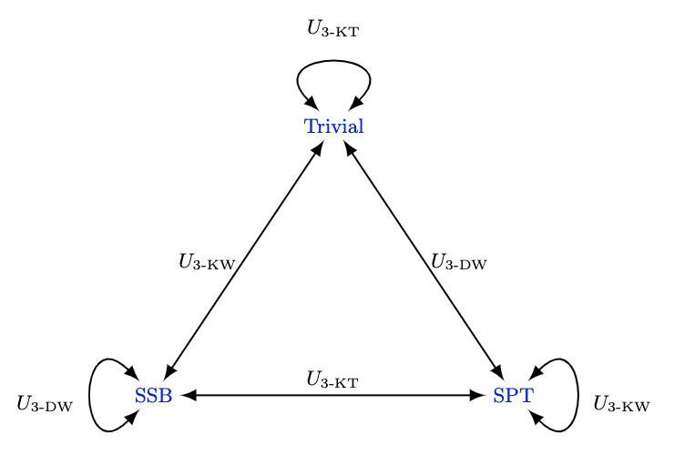
Figure 1: Three gapped phases with $\mathbb{Z}_{2}\times\mathbb{Z}_{2}$ symmetry and the dualities between them.

Here $U_{\text{3-KT}}$ is a generalized Kennedy-Tasaki transformation [23, 91]:

$$U_{\text{3-KT}}=U_{\text{3-DW}}U_{\text{3-KW}}U^{\dagger}_{\text{3-DW}}.$$ (30)

Moreover, such a web of duality can also connect phase transitions between two different gapped phases, as shown in Fig. 2. These duality-related three phase transitions have the same center charge $c=1$.

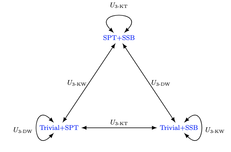
Figure 2: Three phase transitions between two different gapped phases with $\mathbb{Z}_{2}\times\mathbb{Z}_{2}$ symmetry and $c=1$ and the dualities between them.

Lastly, we have constructed another BPM duality example that connects $H=-\sum X_{i}$ and $H=-\sum Z_{i}Z_{i+1}Z_{i+2}Z_{i+3}$ in the appendix. Interestingly, on self-dual points, this duality becomes an anomalous symmetry, which guarantees the self-dual theory must be either a first-order or continuous phase transition.

Summary and Discussion — In this paper, we present the Bilinear Phase Map (BPM), a handy tool in understanding quantum phase transitions and exotic gapped phases. Our approach, expands the Kramers-Wannier (KW) transformation, and explores a broader spectrum of quantum phases, addressing the challenge of unitarity loss in duality transformations. Our analysis leads to the derivation of general non-invertible fusion rules and the discovery of new BPMs in (1+1)D systems, which uncover intricate relationships between SPT and SSB phases. Looking forward, this work opens up several intriguing questions and potential research directions. For example, we plan to extend this analysis to from $\mathbb{Z}_{2}$ to $\mathbb{Z}_{N}$ BPMs in a future work. It also paves the way for exploring the applicability of BPM in higher-dimensional systems and its implications in symmetries of quantum systems. Additionally, the anomaly characteristics of BPMs present a fertile ground for further theoretical exploration, potentially leading to the discovery of new quantum phases and transitions.

Appendix A Symmetry-twisting mapping of three-site BPM duality

In this appendix, we will derive the symmetry-twist sectors of BPM $\mathcal{N}_{\text{3-KW}}$. Similar to the boundary spins in $\{\hat{s}_{i}\}$-system, we also introduce boundary spins $(t_{1},t_{2})\in\{0,1\}^{2}$ in $\{s_{i}\}$-system:

$$\begin{split}&s_{L+3k+1}=s_{3k+1}+t_{A},\quad s_{L+3k+2}=s_{3k+2}+(t_{A}+t_{G}),\quad s_{L+3k}=s_{3k}+t_{G}.\end{split}$$ (31)

Then we find a consistent modified expression of $\mathcal{N}_{\text{3-KW}}$ in $\{s_{i}\}$ and $\{\hat{s}_{i}\}$ systems:

$$\begin{split}\mathcal{N}_{\text{3-KW}}\ket{\{s_{i}\}}&=\frac{1}{2^{\frac{L}{2}}}\sum_{\{\hat{s}_{i}\}}(-1)^{\sum_{j=1}^{L}s_{j}(\hat{s}_{j}+\hat{s}_{j+1}+\hat{s}_{j+2})+t_{A}\hat{s}_{1}+t_{G}\hat{s}_{2}}\ket{\{\hat{s}_{i}\}}\\ &=\frac{1}{2^{\frac{L}{2}}}\sum_{\{\hat{s}_{i}\}}(-1)^{\sum_{j=1}^{L}\hat{s}_{j}(s_{j-2}+s_{j-1}+s_{j})+\hat{t}_{G}s_{L}+\hat{t}_{A}s_{L-1}}\ket{\{\hat{s}_{i}\}}.\end{split}$$ (32)

From this formula, it is straightforward to check the symmetry-twist mapping:

$$\begin{split}[(\hat{u}_{A},\hat{t}_{A}),(\hat{u}_{G},\hat{t}_{G})]=[(t_{A}+t_{G},u_{A}),(t_{G},u_{A}+u_{G})].\end{split}$$ (33)

Let us first acts $\hat{U}_{A}\times\mathcal{N}_{\text{3-KW}}$ and $\hat{U}_{G}\times\mathcal{N}_{\text{3-KW}}$ on the state $\ket{\{s_{i}\}}$:

$$\begin{split}&\hat{U}_{A}\mathcal{N}_{\text{3-KW}}\ket{\{s_{i}\}}=(-1)^{t_{A}+t_{G}}\mathcal{N}_{\text{3-KW}}\ket{\{s_{i}\}},\\ &\hat{U}_{G}\mathcal{N}_{\text{3-KW}}\ket{\{s_{i}\}}=(-1)^{t_{G}}\mathcal{N}_{\text{3-KW}}\ket{\{s_{i}\}}.\end{split}$$ (34)

This holds for any state $N_{\text{3-KW}}|\psi\rangle$, where $|\psi\rangle$ is a general state in $\{s_{i}\}$ system $\ket{\psi}=\sum_{\{s_{i}\}}\psi_{\{s_{i}\}}\ket{\{s_{i}\}}$. Thus any state obtained by acting $N_{\text{3-KW}}$ must be eigenstate of $\hat{U}_{A}$ and $\hat{U}_{G}$ with eigenvalue $(\hat{u}_{A},\hat{u}_{G})=(t_{A}+t_{G},t_{G})$.

Next, we continue to consider $\mathcal{N}_{\text{3-KW}}\times U_{1}$ and $\mathcal{N}_{\text{3-KW}}\times U_{G}$:

$$\begin{split}&\mathcal{N}_{\text{3-KW}}U_{A}\ket{\{s_{i}\}}=(-1)^{\hat{t}_{A}}\mathcal{N}_{\text{3-KW}}\ket{\{s_{i}\}},\\ &\mathcal{N}_{\text{3-KW}}U_{G}\ket{\{s_{i}\}}=(-1)^{\hat{t}_{A}+\hat{t}_{G}}\mathcal{N}_{\text{3-KW}}\ket{\{s_{i}\}}.\end{split}$$ (35)

Similarly, this is valid for general state $|\psi\rangle$. In particular, we can consider an eigenstate $\ket{\Psi}$ of $(U_{A},U_{G})$ with eigenvalue $(u_{A},u_{G})$. Thus we have

$$\begin{split}&\mathcal{N}_{\text{3-KW}}U_{A}\ket{\Psi}=(-1)^{\hat{t}_{A}}N_{\text{3-KW}}\ket{\Psi}=N_{\text{3-KW}}(-1)^{u_{A}}\ket{\Psi},\\ &\mathcal{N}_{\text{3-KW}}U_{G}\ket{\Psi}=(-1)^{\hat{t}_{A}+\hat{t}_{G}}N_{\text{3-KW}}\ket{\Psi}=N_{\text{3-KW}}(-1)^{u_{G}}\ket{\Psi},\end{split}$$ (36)

namely,

$$(u_{A},u_{G})=(\hat{t}_{A},\hat{t}_{A}+\hat{t}_{G}).$$ (37)

Then it follows that $(\hat{t}_{A},\hat{t}_{G})=(u_{A},u_{A}+u_{G})$.

Appendix B SPT phase invariant under three-site BPM duality and Kennedy-Tasaki duality

In this appendix, we will discuss the SPT phase invariant under $\mathcal{N}_{\text{3-KW}}$ and the Kennedy-Tasaki duality between SPT phase and SSB phase.

B.1 The Hamiltonian of SPT phase

Let us begin our discussion with an exactly solvable Hamiltonian with $L\in 6\mathbb{Z}$:

$$H_{\text{SPT}}=-\sum^{L}_{i=1}a_{i},\quad a_{i}=(-1)^{i}Z_{i-1}Y_{i}Z_{i+1}.$$ (38)

It is straightforward to show this Hamiltonian has the $(\mathbb{Z}_{2})^{2}$ symmetry (20) and is invariant under three-site BPM. By a $U_{\text{3-DW}}$ transformation, this SPT Hamiltonian is mapped to a Hamiltonian belonging to the trivially gapped phase:

$$U^{\dagger}_{\text{3-DW}}H_{\text{SPT}}U_{\text{3-DW}}=-\sum^{L}_{i=1}X_{i}=H_{\text{triv}},$$ (39)

where

$$U_{\text{3-DW}}=\prod^{L}_{i=1}\exp(-\frac{\pi i}{4}(-1)^{i}Z_{i})\prod^{L}_{i=1}\exp[\frac{\pi i}{4}(1-Z_{i})(1-Z_{i+1})]T,$$ (40)

and $T$ is one-site lattice translation. The dual Hamiltonian has a unique ground state, thus the Hamiltonian (38) also has a unique gapped ground state.

B.2 String order parameters, ground state charge under twisted boundary condition and edge modes

In this section, we will detect the SPT order by different methods. The first method is the string order parameter:

$$\begin{split}\langle S_{U_{A}}\rangle&=(-1)^{m-n+1}\langle Z_{3n}\prod^{m}_{k=n}(X_{3k+1}X_{3k+2})Z_{3m+3}\rangle=\langle\prod^{m}_{k=n}a_{3k+1}a_{3k+2}\rangle=1,\\ \langle S_{U_{G}}\rangle&=(-1)^{m-n+1}\langle Z_{3n-2}\prod^{m}_{k=n}(X_{3k-1}X_{3k})Z_{3m+1}\rangle=\langle\prod^{m}_{k=n}a_{3k-1}a_{3k}\rangle=1.\end{split}$$ (41)

The string order parameter $S_{U_{A}}$ ($S_{U_{G}}$) is obtained by dressing the string operator of $U_{A}$ ($U_{G}$) symmetry with charged operator of $U_{G}$ ($U_{A}$) symmetry at endpoints, which is consistent with decorated domain wall construction.

The second way to probe the SPT order is ground state charge under twisted boundary conditions on the closed chains. For simplicity, we assume $L\in 6\mathbb{Z}$. Let us first twist the boundary condition using the $\mathbb{Z}_{2}^{A}$ symmetry (labeled by $\mathbb{Z}_{2}^{A}$-TBC), and measure the $\mathbb{Z}_{2}^{G}$ charge of the ground state. Twisting the boundary condition by $\mathbb{Z}_{2}^{A}$ means imposing a domain wall between sites $L-1$ and $1$ by changing the sign of the term $Z_{L-1}Y_{L}Z_{1}$. The SPT Hamiltonian (38) becomes

$$H^{\mathbb{Z}_{2}^{A}}_{\text{SPT}}=\sum^{L-1}_{i=1}a_{i}-a_{L}.$$ (42)

We note that the twisted and untwisted SPT Hamiltonian are related by a unitary transformation $H_{\text{SPT}}^{\mathbb{Z}_{2}^{A}}=Z_{L}H_{\text{SPT}}Z_{L}$. Denote the ground state under PBC as $\ket{\text{GS}}$, and that under $\mathbb{Z}_{2}^{A}$-TBC as $\ket{\text{GS}}_{\text{tw}}^{\mathbb{Z}_{2}^{A}}$. We have

$$\ket{\text{GS}}_{\text{tw}}^{\mathbb{Z}_{2}^{A}}=Z_{L}\ket{\text{GS}}.$$ (43)

It follows that

$$U_{G}\ket{\text{GS}}_{\text{tw}}^{\mathbb{Z}_{2}^{A}}=U_{G}Z_{L}\ket{\text{GS}}=-Z_{L}\ket{\text{GS}}=-\ket{\text{GS}}_{\text{tw}}^{\mathbb{Z}_{2}^{A}}$$ (44)

which shows that $\ket{\text{GS}}_{\text{tw}}^{\mathbb{Z}_{2}^{A}}$ has $\mathbb{Z}_{2}^{G}$ charge 1. Here we used the fact that the ground state under PBC is neutral under $\mathbb{Z}_{2}^{G}$. We can alternatively twist the boundary condition using $\mathbb{Z}_{2}^{G}$ symmetry (labeled by $\mathbb{Z}_{2}^{G}$-TBC), and measure the $\mathbb{Z}_{2}^{A}$ charge of the ground state. By the same method, one can show that the ground state $\ket{\text{GS}}_{\text{tw}}^{\mathbb{Z}_{2}^{G}}$ has odd $\mathbb{Z}_{2}^{A}$ charge.

At last, we will derive how symmetry fractionalizes on edge modes. Let us place the spin system on an open chain with $1\leq i\leq L$ and choose the OBC such that only the interactions completely supported on the chain are kept. The Hamiltonian is

$$H_{\text{SPT}}^{\text{OBC}}=-\sum^{L-1}_{j=2}a_{j}.$$ (45)

There are two boundary terms on each edge: $Z_{1}$, $X_{1}Z_{2}$, $Z_{L}$, $Z_{L-1}X_{L}$. All the operators commute with bulk Hamiltonian and the anticommutation relation of two terms on each edge gives rise to 2-fold degenerate subspace.

To see the symmetry fractionalization, we note that for ground states

$$\begin{split}&\prod^{L/3-1}_{k=1}a_{3k+1}a_{3k+2}=-Z_{3}\prod^{L/3-1}_{k=1}(X_{3k+1}X_{3k+2})Z_{L}=1,\\ &\prod^{L/3-1}_{k=1}a_{3k-1}a_{3k}=-Z_{1}\prod^{L/3-1}_{k=1}(X_{3k-1}X_{3k})Z_{L-2}=1.\end{split}$$ (46)

This implies the symmetry operator fractionalizes as $U_{A/G}=-\mathcal{L}_{A/G}\mathcal{R}_{A/G}$ where

$$\begin{split}&\mathcal{L}_{A}=X_{1}X_{2}Z_{3},\mathcal{R}_{A}=Z_{L},\\ &\mathcal{L}_{A}=Z_{1},\mathcal{R}_{G}=Z_{L-2}X_{L-1}X_{L}.\end{split}$$ (47)

On each edge, the projective representation of $\mathcal{L}$ and $\mathcal{R}$ gives rise to the edge modes. Such symmetry fractionalizes and the resulting edge modes are robust as long as the bulk gap is not closed.

At last, we remark that when $L\notin 3$, the Hamiltonian (38) does not respect $(\mathbb{Z}_{2})^{2}$ symmetry. This is because BPM under PBC only has the trivial kernel $(0,0,0,\cdots)$ and is not associated with $U_{A}$ and $U_{G}$ in this case. Thus the $\mathcal{N}_{3-\text{KW}}$ is a unitary transformation and the Hamiltonian (15) with $h=0$ has a unique ground state.

B.3 The generalized Kennedy-Tasaki transformation

Similar to the reference [23], we can also construct a generalized Kennedy-Tasaki transformation, which can relate the SPT phase (38) and the SSB model $H_{\text{SSB}}=-\sum^{L}_{i=1}Z_{i}Z_{i+1}Z_{i+2}$:

$$U_{\text{3-KT}}=U_{\text{3-DW}}U_{\text{3-KW}}U^{\dagger}_{\text{3-DW}}.$$ (48)

It is straightforward to derive the fusion rule of this KT transformation:

$$\begin{split}U_{\text{3-KT}}U_{\text{3-KT}}&=U_{\text{3-DW}}U_{\text{3-KW}}U_{\text{3-KW}}U^{\dagger}_{\text{3-DW}}\\ &=U_{\text{3-DW}}(1+U_{A})(1+U_{G})T^{2}U^{\dagger}_{\text{3-DW}}\\ &=(1+U_{A})(1+U_{G})T^{2}\end{split}$$ (49)

where we use the fact that $U_{\text{3-DW}}$ commutes with two-site translation and $U_{A}$ and $U_{G}$ operators.

Appendix C Four-site BPM duality transformation

C.1 BPM duality under PBC and fusion rules

In this appendix, we discuss the BPM duality which is related to the following four-site Ising chain with $L\in 4\mathbb{Z}$:

$$\begin{split}H_{\text{4-Ising}}=-\sum^{L}_{i=1}(hX_{i}+Z_{i}Z_{i+1}Z_{i+2}Z_{i+3}).\end{split}$$ (50)

This system has a unique ground state with all $X_{i}=1$ when $h=\infty$, while it is in the SSB phase when $h=0$. To understand the duality between these two phases, we can construct a generalized KW duality under PBC:

$$\begin{split}\mathcal{N}_{\text{4-KW}}\ket{\{s_{i}\}}&=\frac{1}{2^{\frac{L}{2}}}\sum_{\{\hat{s}_{i}\}}(-1)^{\sum_{j=1}^{L}s_{j}(\hat{s}_{j}+\hat{s}_{j+1}+\hat{s}_{j+2}+\hat{s}_{j+3})}\ket{\{\hat{s}_{i}\}}\\ &=\frac{1}{2^{\frac{L}{2}}}\sum_{\{\hat{s}_{i}\}}(-1)^{\sum_{j=1}^{L}\hat{s}_{j}(s_{j-3}+s_{j-2}+s_{j-1}+s_{j})}\ket{\{\hat{s}_{i}\}},\end{split}$$ (51)

whose BPM matrix is :

$${\bf\it A}_{\text{4-KW}}=\left(\begin{array}[]{ccccccc}1&1&1&1&0&\cdots&0\\ 0&1&1&1&1&\cdots&0\\ 0&0&1&1&1&\cdots&0\\ \cdots&\cdots&\cdots&\cdots&\cdots\\ 1&1&0&\cdots&0&1&1\\ 1&1&1&0&\cdots&0&1\\ \end{array}\right).$$ (52)

Similarly, the properties of symmetry and SSB ground state degeneracy can be derived from the kernels of ${\bf\it A}^{T}_{\text{4-KW}}$:

$${\bf\it b}^{1}=(1,0,1,0,1,0,1,0,\cdots),\quad{\bf\it b}^{2}=(0,1,0,1,0,1,0,1,\cdots),\quad{\bf\it b}^{3}=(1,1,0,0,1,1,0,0,\cdots).$$ (53)

This shows the system has a $(\mathbb{Z}_{2})^{3}$ symmetry:

$$U_{o}\ket{\{s_{i}\}}=\ket{\{s_{i}+b^{1}_{i}\}},\quad U_{e}\ket{\{s_{i}\}}=\ket{\{s_{i}+b^{2}_{i}\}},\quad U_{1}\ket{\{s_{i}\}}=\ket{\{s_{i}+b^{3}_{i}\}}.$$ (54)

In operator form, they are given by:

$$\begin{split}&U_{e}=\prod^{L/2}_{i=1}X_{2i},\quad U_{o}=\prod^{L/2}_{i=1}X_{2i+1},\quad U_{1}=\prod^{L/4}_{i=1}X_{4i+1}X_{4i+2}.\end{split}$$ (55)

Thus all states can be organized into eigenstates of $U_{e/o/1}$ with eigenvalue $(-1)^{u_{e/o/1}}=\pm 1$, i.e. $u_{e/o/1}=0,1$.

The eight ground states of the SSB phase can be generated by these symmetry operators from the all spin-up state:

$$\begin{split}&\ket{\text{GS}}_{1}=\ket{\uparrow\uparrow\uparrow\uparrow\cdots},\quad\ket{\text{GS}}_{2}=\ket{\uparrow\downarrow\uparrow\downarrow\cdots},\\ &\ket{\text{GS}}_{3}=\ket{\downarrow\uparrow\downarrow\uparrow\cdots},\quad\ket{\text{GS}}_{4}=\ket{\downarrow\downarrow\downarrow\downarrow\cdots},\\ &\ket{\text{GS}}_{5}=\ket{\downarrow\downarrow\uparrow\uparrow\cdots},\quad\ket{\text{GS}}_{6}=\ket{\downarrow\uparrow\uparrow\downarrow\cdots},\\ &\ket{\text{GS}}_{7}=\ket{\uparrow\downarrow\downarrow\uparrow\cdots},\quad\ket{\text{GS}}_{8}=\ket{\uparrow\uparrow\downarrow\downarrow\cdots}.\end{split}$$ (56)

This BPM duality induces the transformation of Pauli operators

$$\begin{split}&\mathcal{N}_{\text{4-KW}}X_{i}=\hat{Z}_{i}\hat{Z}_{i+1}\hat{Z}_{i+2}\hat{Z}_{i+3}\mathcal{N}_{\text{4-KW}},\\ &\mathcal{N}_{\text{4-KW}}Z_{i-3}Z_{i-2}Z_{i-1}Z_{i}=\hat{X}_{i}\mathcal{N}_{\text{4-KW}},\end{split}$$ (57)

and thus exchanges transverse field term and four-site lsing term. Likewise, the dual Hilbert space can also be organized into four symmetry sectors labeled by $(\hat{u}_{o},\hat{u}_{e},\hat{u}_{1})\in\{0,1\}^{3}$.

We can also determine fusion rules by acting the product of $\hat{U}_{e/o/1}\times\mathcal{N}_{\text{4-KW}}$, $\mathcal{N}_{\text{4-KW}}\times U_{e/o/1}$ and $\mathcal{N}_{\text{4-KW}}\times\mathcal{N}_{\text{4-KW}}$ on a general state:

$$\begin{split}&\mathcal{N}_{\text{4-KW}}\times U_{e/o/1}=\mathcal{N}_{\text{4-KW}},\quad\hat{U}_{e/o/1}\times\mathcal{N}_{\text{4-KW}}=\mathcal{N}_{\text{4-KW}},\\ &\mathcal{N}_{\text{4-KW}}\times\mathcal{N}_{\text{4-KW}}=(1+U_{e})(1+U_{o})(1+U_{1})T^{3}\,.\end{split}$$ (58)

C.2 Unitarity problem and symmetry-twist transformation

To solve this unitarity problem in this case, we need to add three additional boundary spins $t_{e}$, $t_{o}$ and $t_{1}$ in $\{s_{i}\}$-systems and another three spins $\hat{t}_{e}$, $\hat{t}_{o}$ and $\hat{t}_{1}$ in $\{\hat{s}_{i}\}$-systems, i.e. the untwisted/twisted boundary condition of $(\mathbb{Z}_{2})^{3}$ symmetry:

$$\begin{split}&s_{L+4k+1}=s_{4k+1}+(t_{o}+t_{1}),s_{L+4k+2}=s_{4k+2}+(t_{e}+t_{1}),\\ &s_{L+4k+3}=s_{4k+3}+t_{o},\quad s_{L+4k}=s_{4k}+t_{e}.\\ &\hat{s}_{L+4k+1}=\hat{s}_{4k+1}+(\hat{t}_{o}+\hat{t}_{1}),\hat{s}_{L+4k+2}=\hat{s}_{4k+2}+(t_{e}+t_{1}),\\ &\hat{s}_{L+4k+3}=\hat{s}_{4k+3}+\hat{t}_{o},\quad\hat{s}_{L+4k}=\hat{s}_{4k}+\hat{t}_{e}.\end{split}$$ (59)

We also find a consistent modification of BPM:

$$\begin{split}&\mathcal{N}_{\text{4-KW}}\ket{\{s_{i}\}}=\frac{1}{2^{\frac{L}{2}}}\sum_{\{\hat{s}_{i}\}}(-1)^{\sum_{j=1}^{L}s_{j}(\hat{s}_{j}+\hat{s}_{j+1}+\hat{s}_{j+2}+\hat{s}_{j+3})+t_{e}(\hat{s}_{2}+\hat{s}_{3})+t_{o}(\hat{s}_{1}+\hat{s}_{2})+t_{1}\hat{s}_{1}}\ket{\{\hat{s}_{i}\}}\\ &=\frac{1}{2^{\frac{L}{2}}}\sum_{\{\hat{s}_{i}\}}(-1)^{\sum_{j=1}^{L}\hat{s}_{j}(s_{j-3}+s_{j-2}+s_{j-1}+s_{j})+\hat{t}_{o}(s_{L-1}+s_{L-2})+\hat{t}_{e}(s_{L}+s_{L-1})+\hat{t}_{1}s_{L-2}}\ket{\{\hat{s}_{i}\}}.\end{split}$$ (60)

By a similar method, one can find the symmetry-twist mapping from this formula:

$$\begin{split}&[(\hat{u}_{o},\hat{t}_{o}),(\hat{u}_{e},\hat{t}_{e}),(\hat{u}_{1},\hat{t}_{1})]\\ =&[(t_{o}+t_{e}+t_{1},u_{e}+u_{o}+u_{1}),(t_{o}+t_{e},u_{e}+u_{1}),(t_{1}+t_{e},u_{o}+u_{e})].\end{split}$$ (61)

We can apply this modified BPM to fix the unitarity problem for SSB ground states, which satisfies that $s_{j-3}+s_{j-2}+s_{j-1}+s_{j}=0$. The BPM maps them to the paramagnetic state with $\hat{X}_{i}=1$:

$$\frac{1}{2^{\frac{L}{2}}}(-1)^{\hat{t}_{o}(s_{L-1}+s_{L-2})+\hat{t}_{e}(s_{L}+s_{L-1})+\hat{t}_{1}s_{L-2}}\sum_{\{\hat{s}_{i}\}}\ket{\{\hat{s}_{i}\}}.$$ (62)

When $\hat{t}_{o}=\hat{t}_{e}=\hat{t}_{1}=0$, the phase is trivial and only linear combination $\sum^{8}_{i=1}\ket{\text{GS}}_{i}$ with all $u=0$ survives. But when $\hat{t}_{o}=1$ and $\hat{t}_{e}=\hat{t}_{1}=0$, four ground states with $s_{L-1}+s_{L-2}=1$ will be mapped with additional $-1$ sign. Then only linear combination $(\ket{\text{GS}}_{1}+\ket{\text{GS}}_{4}+\ket{\text{GS}}_{6}+\ket{\text{GS}}_{7}-\ket{\text{GS}}_{2}-\ket{\text{GS}}_{3}-\ket{\text{GS}}_{5}-\ket{\text{GS}}_{8})$ survives. This combination has symmetry charge $u_{o}=u_{e}=u_{1}=1$, which is the solution of Eq. (LABEL:eq:sym-twist_map). It is straightforward to check other cases and linear combinations of SSB ground states with different symmetry eigenvalues will be mapped to the paramagnetic state under different boundary conditions, which satisfies the rule of symmetry-twist mapping (LABEL:eq:sym-twist_map).

C.3 Anomaly of four-site BPM duality symmetry

On the self-dual point $h=1$, the model $H_{\text{4-Ising}}$ is at a first-order phase transition between SSB phase and the trivial phase [74, 80]. The BPM duality $\mathcal{N}_{\text{4-KW}}$ also becomes an emergent non-invertible symmetry for the self-dual theory. Such an emergent symmetry is anomalous in the sense that it cannot allow a symmetric uniquely gapped phase under any symmetric perturbations and hence self-dual theories must be always at first-order or second-order first phase transitions.

To prove the anomaly of $\mathcal{N}_{\text{4-KW}}$, let us first show this duality operator can be decomposed as the product under PBC: $\mathcal{N}_{\text{4-KW}}=\frac{1}{2}\mathcal{N}_{\text{KW'}}\times(\mathcal{N}_{\text{KW}})^{\dagger}\times\mathcal{N}_{\text{KW'}}$. Here the $\mathcal{N}_{\text{KW}}$ is the usual KW transformation (1) and $\mathcal{N}_{\text{KW'}}$ is the combination of two KW transformations acting on even and odd sites:

$$\begin{split}&\mathcal{N}_{\text{KW'}}\ket{\{s_{i}\}}=\frac{1}{2^{\frac{L}{2}}}\sum_{\{\hat{s}_{i}\}}(-1)^{\sum_{j,k=1}^{L}(s_{j-2}+s_{j})\hat{s}_{k}}\ket{\{\hat{s}_{i}\}}.\end{split}$$ (63)

We can directly check this result

$$\begin{split}&\mathcal{N}_{\text{KW'}}\times(\mathcal{N}_{\text{KW}})^{\dagger}\times\mathcal{N}_{\text{KW'}}\ket{\{s_{i}\}}\\ =&\frac{1}{2^{\frac{3L}{2}}}\sum_{\{s^{\prime}_{i},s^{\prime\prime}_{i},\hat{s}_{i}\}}(-1)^{\sum^{L}_{j=1}s^{\prime}_{j}(s_{j-2}+s_{j})+s^{\prime}_{j}(s^{\prime\prime}_{j-1}+s^{\prime\prime}_{j})+\hat{s}_{j}(s^{\prime\prime}_{j-2}+s^{\prime\prime}_{j})}\ket{\{\hat{s}_{i}\}}\\ =&\frac{1}{2^{\frac{L}{2}}}\sum_{\{s^{\prime\prime}_{i},\hat{s}_{i}\}}\delta(s_{j-2}+s_{j}+s^{\prime\prime}_{j-1}+s^{\prime\prime}_{j})(-1)^{\sum^{L}_{j=1}\hat{s}_{j}(s^{\prime\prime}_{j-2}+s^{\prime\prime}_{j})}\ket{\{\hat{s}_{i}\}}\\ =&\frac{1}{2^{\frac{L}{2}}}\sum_{\{s^{\prime\prime}_{i}=s_{i}+s_{i-1}+0/1,\hat{s}_{i}\}}(-1)^{\sum^{L}_{j=1}\hat{s}_{j}(s^{\prime\prime}_{j-2}+s^{\prime\prime}_{j})}\ket{\{\hat{s}_{i}\}}\\ =&\frac{2}{2^{\frac{L}{2}}}\sum_{\{\hat{s}_{i}\}}(-1)^{\sum^{L}_{j=1}\hat{s}_{j}(s_{j-3}+s_{j-2}+s_{j-1}+s_{j})}\ket{\{\hat{s}_{i}\}}\\ =&2\mathcal{N}_{\text{4-KW}}\ket{\{\hat{s}_{i}\}}.\end{split}$$ (64)

Now, let us prove the anomaly by the contraction method. We first assume a uniquely gapped system is self-dual under PBC and its ground state $|\psi\rangle$ should be short-range entangled (SRE). Due to symmetry-twist mapping, $|\psi\rangle$ should be even under each $\mathbb{Z}_{2}$ symmetry. If we focus on the $\mathbb{Z}^{e}_{2}\times\mathbb{Z}^{o}_{2}$ symmetry, the possible uniquely gapped phase can only be the $\mathbb{Z}^{e}_{2}\times\mathbb{Z}^{o}_{2}$ SPT phase, since trivially gapped phase is mapped to an SSB phase under this four-site BPM. Then we can perform $(\mathcal{N}_{\text{KW'}})^{\dagger}$ or $\mathcal{N}_{\text{KW'}}$ which both keep the SPT phase invariant [23]. Thus $\mathcal{N}_{\text{KW'}}^{\dagger}|\psi\rangle$ and $\mathcal{N}_{\text{KW'}}|\psi\rangle$ are still ground states of the $\mathbb{Z}^{e}_{2}\times\mathbb{Z}^{o}_{2}$ SPT systems and thus SRE. On the other hand, due to (64), we have

$$\begin{split}\langle\psi|\frac{1}{2}\mathcal{N}_{\text{KW'}}\times\frac{1}{2\sqrt{2}}\mathcal{N}_{\text{KW}}^{\dagger}\mathcal{N}_{\text{KW'}}|\psi\rangle=\langle\psi|\frac{1}{2\sqrt{2}}\mathcal{N}_{\text{4-KW}}|\psi\rangle=e^{i\theta}\end{split}$$ (65)

where we multiply the normalized coefficient $\frac{1}{2\sqrt{2}}$. That is

$$\frac{1}{2\sqrt{2}}\mathcal{N}_{\text{KW}}^{\dagger}\mathcal{N}_{\text{KW'}}|\psi\rangle=e^{i\theta}\frac{1}{2}\mathcal{N}_{\text{KW'}}^{\dagger}|\psi\rangle.$$ (66)

However, the $\mathcal{N}^{\dagger}_{\text{KW}}$ maps the $\mathbb{Z}^{e}_{2}\times\mathbb{Z}^{o}_{2}$ SPT phase to an SSB phase of global spin flip $U_{e}U_{o}$. Thus $\frac{1}{2\sqrt{2}}\mathcal{N}^{\dagger}_{\text{KW}}\mathcal{N}_{\text{KW'}}|\psi\rangle$ is a cat state of SSB phase with even charge of $U_{e}U_{o}$ which is not SRE and that finishes our proof.