Exact Work Distribution and Jarzynski’s Equality of a Relativistic Particle in an Expanding Piston

Abstract

We study the non-equilibrium work in a pedagogical model of relativistic ideal gas. We obtain the exact work distribution and verify the Jarzynski’s equality. In the non-relativistic limit, our results recover the non-relativistic results [Lua et al, J. Phys. Chem. B, 109, 6805(2005)]. We also find that, unlike the non-relativistic case, the work distribution no longer has zeros and the number of collisions in this relativistic gas model is finite. In addition, based on an analysis of the experimental parameters, we conclude that it is difficult to detect the relativistic effects of the work distribution of the ideal gas in a piston system with the current experimental techniques.

I Introduction

The Jarzynski’s equality (JE) [1] is one of the most elegant results in the field of non-equilibrium statistical physics. While being a direct result from Liouvelle’s theorem and supposed to hold in arbitrary Hamiltonian systems including relativistic systems, the work distribution of a relativistic system under an arbitrary work protocol has not been explored so far. In this article, we study the work distribution of a simple relativistic model consisting of only a one-dimensional cylinder, a piston and relativistic ideal gas. Previous work on this model has been done and the JE verified, but in a very limited range of parameters [2] such that the collision only happens no more than once for all particles. Moreover, we still lack the detailed information of work distribution of the system giving rise to various fluctuation theorems, which plays a fundamental role in non-equilibrium statistical physics. A Newtonian approximation of our model [3], however, has yielded analytic results both for the JE and the work distribution, suggesting the solvability in the relativistic regime. Relevant to the non-relativistic ideal gas in a piston, the non-equilibrium work distribution of quantum gas in an expanding piston [4][5] has been studied and the JE verified. It is desirable to extend those studies to the relativistic regime. In this article, we analytically compute the work distribution and verify the JE in this simple setup. Our model can be viewed as a relativistic generalization of the one in Ref. [3] and recovers it in the low-speed and low-temperature limit. Such a toy model would be helpful for understanding more complicated and more realistic systems’ behavior under relativistic conditions. As we will see in this paper, although the work distribution changes drastically in the extreme relativistic regime, the equality itself is independent of the microscopic dynamics. In the following, we will study the non-equilibrium work distribution of relativistic gas in an expanding piston. The results can serve as a pedagogical example and provide intuitive insights to the robustness of the JE. Also, we will show that it is difficult to detect the relativistic effect of the work distribution with the current experimental techniques.

The article is organized as follows: In Sec. II, we demonstrate the validity of the JE under the framework of relativistic mechanics. In Sec. III, we analytically calculate the work distribution of a relativistic particle in an expanding piston system. In the non-relativistic limit, we recover the results in Ref. [3]. In Sec. IV, we give the discussion and summary.

II Jarzynski’s equality under the framework of relativistic mechanics

The original proof of the JE was based mainly on the classical Hamilton mechanics and its corollary, i. e., Liouville’s theorem [1]. In this section, we extend the proof to the framework of relativistic mechanics. We take the spacetime dimension to be $1+1$ to suit our model. Note that the generalization to higher spacetime dimensions is straightforward. The manifestly covariant dynamics for a particle of the static mass $m$ can be formulated as

$$f^{\mu}=m\frac{\mathrm{d}u^{\mu}}{\mathrm{d}\zeta},$$ (1)

where $f^{\mu},\,u^{\mu},\,\zeta$ denote the 2-force, 2-velocity and proper time respectively. To be clear, we fix our frame of reference to the laboratory frame, where the relativistic dynamics can be expressed more conveniently in the form of a 1-vector,

$$-\frac{\partial V}{\partial q}=\frac{\mathrm{d}}{\mathrm{d}t}\left(\frac{mu}{\sqrt{1-u^{2}/c^{2}}}\right),$$ (2)

where $V$ denotes the potential, $c$ the speed of light, and $q,u,t$ are the position, velocity and time measured in the laboratory frame. With this form of dynamics, we can easily construct the Hamiltonian of a system of $N$ particles of mass $m_{1},\,m_{2},\,...,\,m_{N}$. Furthermore, we let the Hamiltonian be controlled by an external agent via the parameter $\lambda=\lambda(t)$ of the potential $V_{\lambda}.$ The Hamiltonian reads

$$H_{\lambda}=\sum_{i=1}^{N}\sqrt{m_{i}^{2}c^{4}+p_{i}^{2}c^{2}}+V_{\lambda}(q_{1},\,q_{2},\,...,\,q_{N}),$$ (3)

where $q_{i}$ is the position of the $i$-th particle and $p_{i}$ its conjugate momentum.

The canonical equations are

$$\frac{\mathrm{d}q_{i}}{\mathrm{d}t}=\frac{\partial H_{\lambda}}{\partial p_{i}}=\frac{p_{i}c^{2}}{\sqrt{m_{i}^{2}c^{4}+p_{i}^{2}c^{2}}},$$ (4)

$$\frac{\mathrm{d}p_{i}}{\mathrm{d}t}=-\frac{\partial H_{\lambda}}{\partial q_{i}}=-\frac{\partial V_{\lambda}}{\partial q_{i}},$$ (5)

which is exactly the relativistic velocity-momentum relation that reproduces Eq. (2).

As long as the canonical equations are formulated, one can easily generalize Liouville’s theorem to relativistic regime [6]. The theorem states that the Jacobian determinant of the canonical coordinates $(p_{i,t},q_{i,t})$ at time $t$ as functions of the initial canonical coordinates $(p_{i,0},q_{i,0})$ at time $0$ is

$$\left|\frac{\partial(p_{i,t},q_{i,t})}{\partial(p_{i,0},q_{i,0})}\right|=1.$$ (6)

The initial equilibrium state of the inverse temperature $\beta$ is determined by a probability distribution $\rho(p_{i,0},q_{i,0})=\exp{[-\beta H(p_{i,0},q_{i,0})]}/Z_{0}$ with $Z_{0}=\int\mathrm{d}p_{i,0}\mathrm{d}q_{i,0}\exp[-\beta H_{\lambda(0)}(p_{i,0},q_{i,0})]$ being the initial partition function. We will see in the following (Subsec. III.2) that for ideal gas the distribution is the so-called Maxwell-Jüttner distribution [7]. The proof of the JE follows by calculating the expectation value of the exponential work $\exp{[W(p_{i},q_{i},\tau)]}$ done by the system along the trajectory up to time $\tau.$ By definition we have

$$W(p_{i,0},q_{i,0},\tau)=H_{\lambda(0)}(p_{i,0},q_{i,0})-H_{\lambda(\tau)}(p_{i,\tau},q_{i,\tau})).$$ (7)

Note that our definition is different from the usual one by a minus sign. So

$$\begin{split}&\left\langle e^{\beta W}\right\rangle\\ &=\int\mathrm{d}p_{i,0}\mathrm{d}q_{i,0}\,\rho(p_{i,0},q_{i,0})e^{\beta W(p_{i,0},q_{i,0},\tau)}\\ &=\frac{1}{Z_{0}}\int\mathrm{d}p_{i,0}\mathrm{d}q_{i,0}\,e^{-\beta H_{\lambda(\tau)}(p_{i,\tau},q_{i,\tau})}\\ &=\frac{1}{Z_{0}}\int\mathrm{d}p_{i,\tau}\mathrm{d}q_{i,\tau}\,e^{-\beta H_{\lambda(\tau)}(p_{i,\tau},q_{i,\tau}))}\\ &=\frac{Z_{\tau}}{Z_{0}},\end{split}$$ (8)

where the Liouville’s theorem is used for the third equality and $Z_{\tau}$ denotes the final equilibrium state partition function. The partition functions can be expressed in the form of free energy (see, for example, [8]), resulting in

$$\left\langle e^{\beta W}\right\rangle=e^{-\beta(F_{\tau}-F_{0})},$$ (9)

where $F_{\tau}$ and $F_{0}$ are the free energy of the equilibrium states corresponding to $\lambda(\tau)$ and $\lambda(0)$. Thus, we demonstrate the validity of the JE under the framework of relativistic mechanics.

III A Relativistic Piston Model

The model we consider here is nothing more than some ideal gas inside a one-dimensional cylinder. Suppose initially the length of the vessel is $L$, and the gas is of the inverse temperature $\beta$. We now expand the piston outwards at the speed $v_{p}$, and stop it after a time interval $\tau$.

Under the assumption that the gas is ideal, all particles contribute to both the work $W_{\tau}$ done by the system up to time $\tau$ and the difference between the final and the initial free energy $\Delta F$ independently. Consequently, the JE can be rewritten as

$$(\langle e^{W_{1}/k_{B}T}\rangle)^{N}=(e^{-\Delta F_{1}/k_{B}T})^{N},$$ (10)

where $W_{1}$ and $\Delta F_{1}$ denote the work and the change of the free energy per particle. We can now see that for the ideal gas, the single-particle quantities $W_{1}$ and $\Delta F_{1}$ also satisfy the JE. Thus, we limit our ideal gas to just a single particle, and from now on we omit the subscript $1$ for the discussion of the single-particle quantities.

III.1 Trajectory of a Single Particle

To calculate the trajectory work as a function of the initial state, one must at first figure out how the trajectory of a single particle is like.

Let us denote the velocity of the particle after the $n$-th collision with the moving piston as $v_{n}.$ Following the moving of a particle, we find out that after the $(n+1)$-th collision with the moving piston, the speed of the particle is reduced to

$$v_{n+1}=\frac{(c^{2}+v_{p}^{2})v_{n}-2v_{p}c^{2}}{c^{2}+v_{p}^{2}-2v_{p}v_{n}}.$$ (11)

This result can be derived simply by performing Lorentz transformation twice, noting that the piston is an inertial reference frame during the whole process and the collisions are elastic collisions. The solution to the recurrence relation of the particle’s speed $v_{n}$ after the $n$-th collision can also be derived

$$v_{n}=\frac{(c+v)\alpha_{p}^{2n}-c+v}{(c+v)\alpha_{p}^{2n}+c-v}\cdot c,$$ (12)

where $v$ is the initial speed of the particle and $\alpha_{p}$ is a parameter pertaining to the velocity $v_{p}$ of the moving piston,

$$\alpha_{p}=\frac{c-v_{p}}{c+v_{p}}.$$ (13)

Another thing we must figure out is the time $t_{n}$ when the $n$-th collision with the moving piston takes place. We have the recurrence relation

$$t_{n+1}=\frac{2L+(v_{p}+v_{n})t_{n}}{v_{n}-v_{p}},$$ (14)

from which we can derive the expression of $t_{n}$,

$$\begin{split}t_{n}=\frac{2L}{v_{n-1}-v_{p}}\left(1+\sum_{i=2}^{n-1}\prod_{j=i}^{n-1}\frac{v_{j}+v_{p}}{v_{j-1}-v_{p}}\right)\\ +\left(\prod_{j=1}^{n-1}\frac{v_{j}+v_{p}}{v_{j-1}-v_{p}}\right)\cdot\frac{(L\pm x)}{v_{n-1}-v_{p}}.\end{split}$$ (15)

Here $x$ denotes the initial position of the particle. Note that the sign of $x$ can be either positive or negative due to the initial velocity can be either towards or away from the moving piston. So from now on we simply extend the range of $x$ from $[0,L]$ to $[-L,L]$ to remove the negative sign (for details, please see Appendix A). With the expression of $v_{n}$, the product of a sequence can be simplified

$$\prod_{j=1}^{n}\frac{v_{j}+v_{p}}{v_{j-1}-v_{p}}=2\alpha_{p}^{n}\left[1+\alpha_{p}^{2n}+(-1+\alpha_{p}^{2n})\frac{v}{c}\right].$$ (16)

Finally, we have

$$\begin{split}t_{n}=&\left[(-\alpha_{p}^{2n}-\alpha_{p}+\alpha_{p}^{n+1}+\alpha_{p}^{n})\frac{v}{c}\right.\\ &\left.+(-\alpha_{p}^{n+1}+\alpha_{p}^{n})\frac{x}{L}+(\alpha_{p}-\alpha_{p}^{2n})\right]\\ &\left[-\alpha_{p}+\alpha_{p}^{2n}+(\alpha_{p}+\alpha_{p}^{2n})\frac{v}{c}\right]^{-1}\cdot\frac{L(1+\alpha_{p})}{c(1-\alpha_{p})},\end{split}$$ (17)

which is the time of the $n$-th collision between the particle and the moving piston. It is obvious that $n$ can not take an arbitrarily large number, and the $n$-th collision is guaranteed if and only if both

$$t_{n}\leq\tau\,\mathrm{and}\,v_{n-1}>v_{p}$$ (18)

are fulfilled.

The first requirement ensures that the collision happens before the ending time $\tau$, and the second that the particle can catch up with the moving piston. These requirements give a maximum number of collisions

$$n\leq N=\left[-\frac{\log\left(1+\frac{v_{p}\tau}{L}\right)}{\log\alpha_{p}}\right]+1,$$ (19)

where $[\cdots]$ denotes the integer part of $\cdots.$

Having obtained the number of collisions of every trajectory, we are able to calculate the trajectory work which is a functional of the trajectory and can be determined by the difference of the initial and the final energy of the system.

III.2 A Direct Verification of Jarzynski’s Equality in the Expanding Relativistic Piston Model

It is worth emphasizing that the model we considered here is not characterized by a time-dependent Hamiltonian, but by a parameterized boundary condition [9]. Thus the proof of the JE in Sec. II is inapplicable to the expanding rigid piston system. Still, we can demonstrate that the JE is valid in the expanding rigid piston system. In order to do so, we focus on the Jacobian determinant between the initial and the final state and show it to be unity.

Unlike the case of the low-speed limit, where the initial state satisfies the classical Maxwellian distribution, now the initial state distribution (Maxwell-Jüttner distribution [7]) at the temperature $T=1/(k_{B}\beta)$ is

$$f(x,p)=\frac{1}{2K_{1}(\frac{mc^{2}}{k_{B}T})mcL}e^{-\frac{mc^{2}}{k_{B}T}\sqrt{1+(\frac{p}{mc})^{2}}},$$ (20)

where $K_{1}$ is the modified Bessel function of the second kind, $(x,p)$ are the initial position and the initial momentum, and $k_{B}$ is the Boltzmann’s constant. This distribution can also be expressed in the position-velocity space, with the initial velocity denoted by $v$, as

$$F(x,v)=\frac{1}{2K_{1}(\frac{mc^{2}}{k_{B}T})cL}e^{-\frac{mc^{2}}{k_{B}T}\left(1-\frac{v^{2}}{c^{2}}\right)^{-\frac{1}{2}}}\left(1-\frac{v^{2}}{c^{2}}\right)^{-\frac{3}{2}}.$$ (21)

The exponential work can be averaged over the initial distribution

$$\langle e^{W/k_{B}T}\rangle=\frac{\int_{0}^{L}\mathrm{d}x\int_{-\infty}^{\infty}\mathrm{d}p\,e^{-\frac{mc^{2}}{k_{B}T}\sqrt{1+\left(\frac{p}{mc}\right)^{2}}}e^{W_{\tau}/k_{B}T}}{2K_{1}(\frac{mc^{2}}{k_{B}T})mcL}.$$ (22)

Here $W_{\tau}$ can be uniquely determined by the initial state $(x,p)$.

What can be easily derived from our analysis is that a particle with an initial momentum $p$ can hit the moving piston for $n$ times and its momentum diminishes to

$$p_{n}=\frac{mv_{n}}{\sqrt{1-\left(\frac{v_{n}}{c}\right)^{2}}}.$$ (23)

It is clear to see that the initial state, $(x,p)$, turns into the final state

$$(x_{\tau},p_{\tau})=(|L-v_{n}\tau+(v_{n}+v_{p})t_{n}|,p_{n})$$ (24)

at time $\tau.$ The Jaccobian determinant can be directly computed from Eq. (24),

$$\left|\frac{\partial(p_{\tau},x_{\tau})}{\partial(p,x)}\right|=1,$$ (25)

and thus the JE can be verified in this expanding piston model.

III.3 Distribution of Work

There are three dimensionless parameters in our model: $k_{B}T/(mc^{2}),$ $L/(c\tau)$ and $v_{p}/c.$ Therefore it is convenient to set $m=c=k_{B}=L=1,$ leaving only $v_{p},$ $\tau$ and $\beta=1/T$ as free parameters.

Using the probability distribution Eq. (21), we can evaluate the distribution of work $W$

$$P(W)=\int_{-1}^{1}\mathrm{d}x\int_{0}^{1}\mathrm{d}v\frac{e^{-\frac{\beta}{\sqrt{1-v^{2}}}}\delta(W-W_{\tau}(x,v))}{2K_{1}(\beta)(1-v^{2})^{\frac{3}{2}}},$$ (26)

where $W_{\tau}=1/\sqrt{1-v^{2}}-1/\sqrt{1-v_{n}^{2}}$ is the work done by the particles that have experienced $n$ collisions.

After some tedious calculations (see Appendix B for details), the distribution function of $W$ can be analytically expressed as

$$\begin{split}P(W)=&P_{0}\delta(W)+\frac{1}{2K_{1}(\beta)}\sum_{n=1}^{N}\varphi_{n}(v_{n}(W))\\ \times&\frac{e^{-\beta/\sqrt{1-v_{n}(W)^{2}}}}{(\alpha_{p}^{-n}-1)\left[1+\alpha_{p}^{n}-v_{n}(W)(1-\alpha_{p}^{n})\right]}.\end{split}$$ (27)

Here the overlap factor $\varphi_{n}(v)$ is a trapezoid-shaped function

$$\varphi_{n}(v)=\begin{cases}1-\xi_{n}(v),&\frac{X_{n}-1}{T_{n}}<v_{n}(W)\leq\frac{X_{n}+1}{T_{n}}\\ 2,&\frac{X_{n}+1}{T_{n}}<v_{n}(W)\leq\frac{X_{n+1}-1}{T_{n+1}}\\ 1+\xi_{n+1}(v),&\frac{X_{n+1}-1}{T_{n+1}}<v_{n}(W)\leq\frac{X_{n+1}+1}{T_{n+1}}\end{cases},$$ (28)

where $v_{n}$ as an inverse function of $W_{\tau}$ can be expressed as

$$\begin{split}&v_{n}(W)=\\ &\frac{(1-\alpha_{p}^{n})^{3}(1+\alpha^{n}_{p})+4W\sqrt{\alpha_{p}^{3n}\left((1-\alpha_{p}^{n})^{2}+\alpha_{p}^{n}W^{2}\right)}}{(1-\alpha_{p}^{2n})^{2}+4\alpha_{p}^{2n}W^{2}},\end{split}$$ (29)

and

$$\xi_{n}(v)=-T_{n}v+X_{n},$$ (30)

with

$$T_{n}=\frac{\alpha_{p}^{-(n-1)}-1-\alpha_{p}+\alpha_{p}^{n}}{1-\alpha_{p}}+\frac{\alpha_{p}^{-(n-1)}+\alpha_{p}^{n}}{1+\alpha_{p}}\cdot\tau,$$ (31)

$$X_{n}=\frac{\alpha_{p}^{-(n-1)}-\alpha_{p}^{n}}{1-\alpha_{p}}+\frac{\alpha_{p}^{-(n-1)}-\alpha_{p}^{n}}{1+\alpha_{p}}\cdot\tau.$$ (32)

Here, $\xi_{n}(v)$ is a function of $v$ and denotes the initial position of the particles that happen to collide with the moving piston exactly $n$ times within time $\tau$ with the initial velocity $v$. For a pictorial explanation, please see Appendix B. Note that $\xi_{n}(v)$ is a linear function of $v$. This is not as obvious as in the non-relativistic regime. For an intuitive explanation, please see Appendix A.

Just like the case in Newtonian mechanics, we expect the work distribution to have a Dirac $\delta$ peak at $W=0$. Its amplitude can be simply evaluated as

$$P_{0}=\int_{0}^{1}\mathrm{d}v\frac{\varphi_{0}(v)e^{-\frac{\beta}{\sqrt{1-v^{2}}}}}{2K_{1}(\beta)(1-v^{2})^{\frac{3}{2}}},$$ (33)

where the overlap function $\varphi_{0}(v)$ is piecewise linear. It can be evaluated analytically, although it is quite involved.

III.4 Non-relativistic Limit

In the non-relativistic limit, we expect our results to recover those in Ref. [3]. For our choice of units, where the speed of light is set to be 1, the Newtonian mechanics is recovered by taking $v_{p}\ll 1$ and $W\sim 1/\beta\sim v_{p}^{2}.$

We will deal with the exponential part in Eq. (27) separately. For now we can expand the rest part of the work distribution except the exponential and the normalization constant at $v_{p}$ around $0$ and $W$ around $0.$ We have

$$\begin{split}&[1-\xi_{n}(v_{n}(W))]\cdot\frac{1}{(\alpha_{p}^{-n}-1)\left[1+\alpha_{p}^{n}-v_{n}(W)(1-\alpha_{p}^{n})\right]}\\ &=-\frac{n-1}{2nv_{p}}-\frac{(n-1)\tau}{4n}+\frac{\tau W}{8n^{2}v_{p}^{2}}+O(v_{p}^{2}),\end{split}$$ (34)

$$2\cdot\frac{1}{(\alpha_{p}^{-n}-1)\left[1+\alpha_{p}^{n}-v_{n}(W)(1-\alpha_{p}^{n})\right]}=\frac{1}{2nv_{p}},$$ (35)

and

$$\begin{split}&[1+\xi_{n+1}(v_{n}(W))]\cdot\frac{1}{(\alpha_{p}^{-n}-1)\left[1+\alpha_{p}^{n}-v_{n}(W)(1-\alpha_{p}^{n})\right]}\\ &=\frac{n+1}{2nv_{p}}+\frac{(n+1)\tau}{4n}-\frac{\tau W}{8n^{2}v_{p}^{2}}+O(v_{p}^{2})\end{split}$$ (36)

as all pieces of the trapezoid-shaped function $\varphi_{n}.$

The exponential term left in Eq. (27), together with the normalization constant $K_{1}(\beta)$, needs to be treated with extra care. We start by noting that the thermodynamic temperature $\beta$ is of the order $v_{p}^{-2},$ so

$$-\frac{\beta}{\sqrt{1-v_{n}(W)^{2}}}=-\beta-\frac{\beta}{2}\left(\frac{W}{2nv_{p}}+nv_{p}\right)^{2}+O(v_{p}),$$ (37)

where a temperature dependent constant $e^{-\beta}$ appears. The low-temperature limit also affects the constant factors, yielding

$$\frac{e^{-\beta}}{K_{1}(\beta)}\approx\sqrt{\frac{2\beta}{\pi}}$$ (38)

as $\beta$ approaches $\infty$, which is exactly the Maxwellian normalization constant.

To conclude, we are able to recover the non-relativistic results in Ref. [3] ( $\tau=1$ is chosen in accordance with Ref. [3] )

$$P(W)=\frac{\sqrt{\beta}}{\sqrt{2\pi}nv_{p}}e^{-\frac{\beta}{2}(\frac{W}{2nv_{p}}+nv_{p})^{2}}f(W),$$ (39)

with

$$f(W)=\begin{cases}-(n-1)(1+\frac{v_{p}}{2})+\frac{W}{4nv_{p}},&(n-1)(v_{p}+2)<\frac{W}{2nv_{p}}\leq(n-1)(v_{p}+2)+2\\ 1,&(n-1)(v_{p}+2)+2<\frac{W}{2nv_{p}}\leq(n-1)(v_{p}+2)+2+2v_{p}\\ (n+1)(1+\frac{v_{p}}{2})-\frac{W}{4nv_{p}},&(n-1)(v_{p}+2)+2+2v_{p}<\frac{W}{2nv_{p}}\leq(n+1)(v_{p}+2)\end{cases}$$ (40)

as a low-speed limit.

In Fig. 1(a)-3(a) we plot the work distributions of the expanding relativistic piston model and its non-relativistic limit. The deviations of the relativistic results from the non-relativistic ones with different choices of parameters are shown. One can see that as expected, the relativistic results deviate more prominently from the non-relativistic results at high temperature and fast speed.

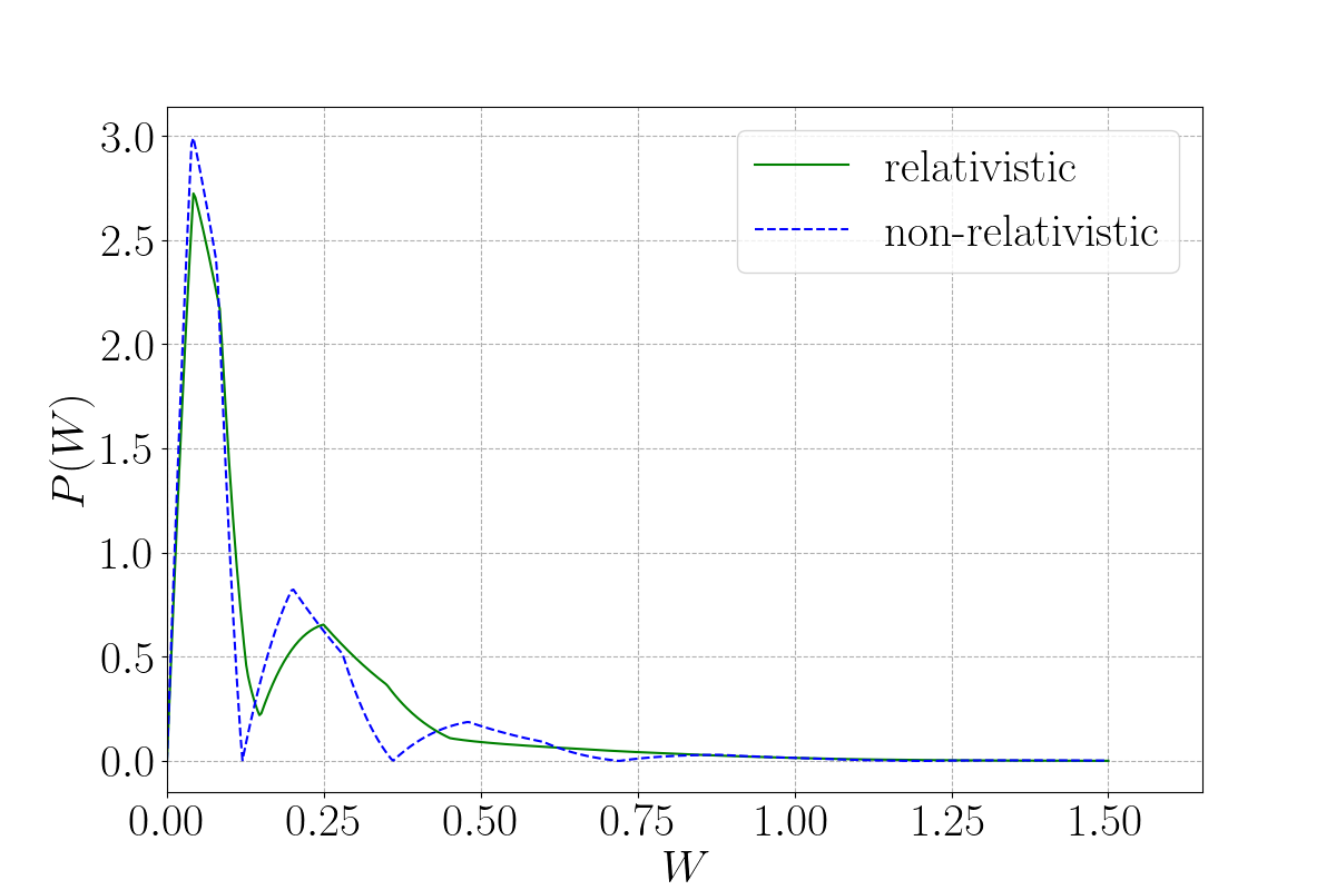
(a) $\tau=10,\,v_{p}=0.1,\,\beta=3$

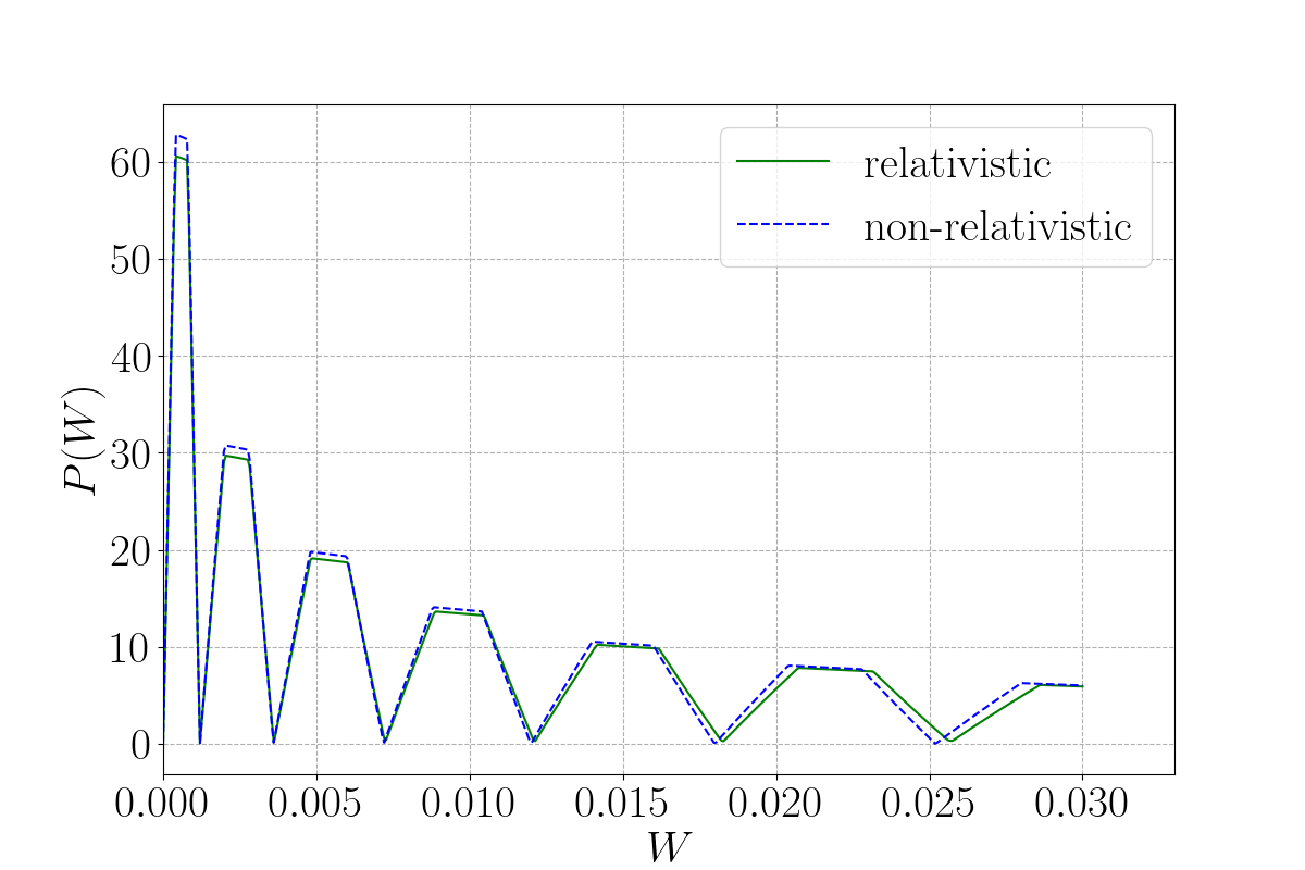
(a) $\tau=100,\,v_{p}=0.01,\,\beta=10$

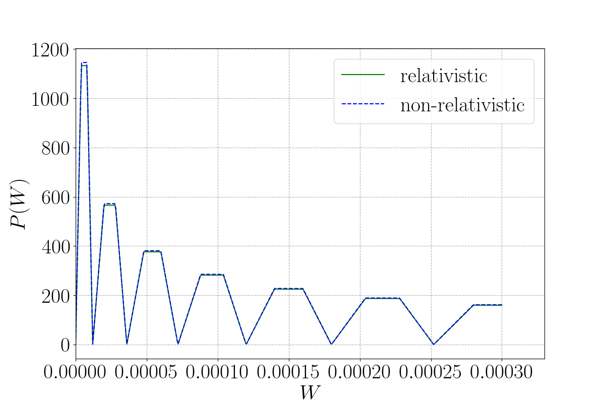
(a) $\tau=1000,\,v_{p}=0.001,\,\beta=33$

Figure 3: Relativisitic and non-relativistic work distribution with different parameters. Take hydrogen atoms as an example. Supposing that the length of the cylinder is $L=1\mathrm{cm}$ (which is much larger than the thermal length of the atoms). The parameters are chosen to be $\tau=0.3\mathrm{ns},v_{p}=3\times 10^{7}\mathrm{m/s},T=3\times 10^{12}\mathrm{K}$ in (a), $\tau=3\mathrm{ns},v_{p}=3\times 10^{6}\mathrm{m/s},T=1\times 10^{12}\mathrm{K}$ in (b), and $\tau=30\mathrm{ns},v_{p}=3\times 10^{5}\mathrm{m/s},T=3\times 10^{11}\mathrm{K}$ in (c).

III.5 Limit of Fast-moving Piston

We have already known that in Newtonian mechanics, at a very large $v_{p}$, the validity of the JE relies on the far tails of the Maxwellian distribution [3]. It is thus intriguing to also think of this problem in special relativity, where every speed has the speed of light $c$ as its upper bound. The main obstacle to the application of the JE is that to measure the average of exponential work, one must repeat the experiment a certain number of times. The exponent makes sure that the contribution of the tail of the distribution, while its probability goes to zero, is non-vanishing [10]. Specifically in our model, when the speed of the moving piston approaches the speed of light, the fraction of particles that can collide with the piston approaches 0. In such a case an experiment with non-zero work is of probability

$$P(W>0)=\int_{v_{p}}^{1}\mathrm{d}v\frac{\varphi_{1}(v)e^{-\frac{\beta}{\sqrt{1-v^{2}}}}}{2K_{1}(\beta)(1-v^{2})^{\frac{3}{2}}}.$$ (41)

The expectation value of the exponential work is

$$\begin{split}\left\langle e^{\beta W}\right\rangle&=P_{0}\cdot e^{\beta\cdot 0}\\ &+\int_{v_{p}}^{1}\mathrm{d}v\frac{\varphi_{1}(v)e^{-\frac{\beta}{\sqrt{1-v^{2}}}}}{2K_{1}(\beta)(1-v^{2})^{\frac{3}{2}}}\cdot e^{\beta W}.\end{split}$$ (42)

The first term is approximately equal to 1 ($P(W>0)\ll 1$, $P_{0}\approx 1$). From the value of $\exp{(-\beta\Delta F)}=1+v_{p}\tau$, one can expect that, although the probability $P(W>0)$ is vanishingly small, the contribution of the second term is non-zero. This result can be demonstrated transparently in the low-temperature limit. Noticing that

$$\begin{split}e^{-\beta(1-v^{2})^{-\frac{1}{2}}}\cdot e^{\beta W}=&e^{-\beta H_{\lambda(0)}}\cdot e^{\beta(H_{\lambda(0)}-H_{\lambda(\tau)})}\\ =&e^{-\beta H_{\lambda(\tau)}}\\ =&e^{-\beta(1-v_{1}^{2})^{-\frac{1}{2}}},\end{split}$$ (43)

with $v_{1}$ derived from Eq. (12), the particles with small $v_{1}$ after one collision contribute the most to the exponential work. When $v_{1}=0$, the corresponding initial velocity is $2v_{p}/(1+v_{p}^{2})$.

When $\beta\to\infty$, $e^{-\beta(1-v^{2}_{1}(v))^{-\frac{1}{2}}}$ becomes a Gaussian peak, which is a $\delta$ distribution around $v=2v_{p}/(1+v_{p}^{2})$,

$$\begin{split}e^{-\beta(1-v^{2}_{1}(v))^{-\frac{1}{2}}}\approx&e^{-\beta}\sqrt{\frac{2\pi}{\beta}}\delta(v_{1}(v))\\ =&e^{-\beta}\sqrt{\frac{2\pi}{\beta}}\left[1-\left(\frac{2v_{p}}{1+v_{p}^{2}}\right)^{2}\right]\delta\left(v-\frac{2v_{p}}{1+v_{p}^{2}}\right).\end{split}$$ (44)

Together with Eq. (38) and Eq. (28), the second term in Eq. (42) becomes

$$\begin{split}&\int_{v_{p}}^{1}\mathrm{d}v\frac{e^{-\beta}\sqrt{\frac{2\pi}{\beta}}\left[1-\left(\frac{2v_{p}}{1+v_{p}^{2}}\right)^{2}\right]\delta\left(v-\frac{2v_{p}}{1+v_{p}^{2}}\right)}{2e^{-\beta}\sqrt{\frac{\pi}{2\beta}}}\frac{\varphi_{1}(v)}{(1-v^{2})^{\frac{3}{2}}}\\ =&\left[1-\left(\frac{2v_{p}}{1+v_{p}^{2}}\right)^{2}\right]^{-\frac{1}{2}}\varphi_{1}\left(\frac{2v_{p}}{1+v_{p}^{2}}\right)\\ =&v_{p}\tau.\end{split}$$ (45)

This result demonstrates that when the piston moves at a very large $v_{p}$, particles with high initial velocities around $2v_{p}/(1+v_{p}^{2})$ contribute most significantly to the exponential work even if the probability is extremely small. Please note that in Newtonian mechanics particles with initial velocities around $2v_{p}$ contribute most significantly to the exponential work [4][10], even if the probability is extremely small. It can be seen that the results of the relativistic piston model recover those of the non-relativistic piston model as expected.

IV Discussion and Summary

Let us look further into the main results we obtained. We see that, as a consequence of the relativistic energy-velocity relation, the trapezoid-shaped work distribution no longer has a series of zeros. Moreover, the number of peaks becomes finite because the speed of light places an upper bound on all speeds. The apparent paradox of the fast-moving piston in Ref. [3] can be reformulated as when the piston is moving at the speed of light instead of infinity. No particle would be able to catch up with the piston and the average exponential work is unity whereas the free energy change is non-zero. We would like to point out that although light-like worldlines exist, we can not make it stop before and after the moving time period, because such a worldline configuration would violate causality. The best we can do is to take the limiting process of letting the speed of the piston approach the speed of light. Then the order of limit becomes crucial, as we have to integrate out the work $W$ to infinity, and then take the speed limit [4]. This limiting procedure ensures the validity of the JE.

In order to observe a distinct deviation of the relativistic work distribution from its non-relativistic limit, the speed of the piston should be large enough and the temperature of the ideal gas should be extremely high. Take hydrogen atoms as an example, to observe the features of the relativistic work distribution, the piston should be as fast as about $3\times 10^{6}\mathrm{m/s}$, and the temperature of the atoms should be about $10^{12}\mathrm{K}$. When the speed of the piston is about $3\times 10^{5}\mathrm{m/s}$ (faster than the Parker Solar Probe, which is the fastest object human ever built) and the temperature of the atoms is $10^{11}\mathrm{K}$($10^{4}$ times hotter than the central temperature of the Sun), the deviation of the relativistic work distribution from the non-relativistic result becomes barely detectable. Even in such a circumstance, the boundary condition is still difficult to be realized. Because the energy scale of the kinetic energy of the atoms is much larger than the energy scale of the chemical bond, the boundary can not be built by any materials we have already discovered. Based on these facts, we conclude that it is difficult to detect the relativistic effects of the work distribution of ideal gas in a piston system with the current experimental techniques.

In summary, we study a simple model of a piston and ideal gas in the framework of the special theory of relativity. We obtain an analytical result of the work distribution (27) and verify the JE. Using our result it is possible to see the deviation of relativistic work distribution (27) from the non-relativistic one (39) [3]. In principle, these relativistic corrections become non-negligible in the high-temperature and fast-speed limit. However, the range of parameters where relativistic effects are observable would already be far beyond the current experimental techniques. Our results show that the JE holds true in a wide range of systems with generality and serve the pedagogical purpose.

Appendix A A Covariant Description of the Trajectory

In Eq. (15), we extend the range of the initial position $x$ from $[0,L]$ to $[-L,L]$ in order to remove the negative sign related to the direction of $v$. We also notice that in Eq. (30), when $t_{n}$ happens to be $\tau$, the critical initial position and the initial velocity satisfy a linear relation. We will introduce a coordinate transformation method to describe the trajectory of a particle, which will provide pictorial intuition of the two facts.

To begin with, let us consider the collision between the particle and the fixed boundary. In the reference frame of the fixed boundary (which is the same as the laboratory frame), the coordinate frame consists of $x$-axis and $t$-axis, and the world line of the moving piston is $l$ (see Fig. 4(a)). We could draw an auxiliary world line of the moving piston, named $l^{\prime}$. The auxiliary world line $l^{\prime}$ and the real world line $l$ are mirror-symmetric about the $t$-axis. The world line of the particle is a polyline line $I-A-B$. Point $I$ denotes the initial condition of the particle, point $A$ denotes the collision event between the particle and the fixed boundary, and point B denotes the next collision event between the particle and the moving piston. Transformation of the particle’s world line works as follows: the auxiliary event of event $B$ is point $B^{\prime}$. $B$ and $B^{\prime}$ are mirror-symmetric about the $t$-axis. The auxiliary world line of the particle is $I-A-B^{\prime}$. The real world line’s $AB$ part and the auxiliary world line’s $AB^{\prime}$ part are also mirror-symmetric about the $t$-axis. As a result of such transformation, the auxiliary world line of the particle $I-A-B^{\prime}$ is a straight line, which eliminates the world line’s direction change during a collision. Meanwhile, in the frame of the fixed boundary, the auxiliary collision event $B^{\prime}$ has the same time coordinate as event $B$. Therefore, we could use an auxiliary event to evaluate the time when a real collision takes place.

We may also map the initial condition $I(x,-v)$ to an auxiliary initial condition $I^{\prime}(-x,v)$, which is the same as the treatment for Eq. (15). The real motion is that a particle starts from the initial position $I$ with a positive initial position $x$ but a negative initial velocity $-v$ (the particle moves away from the moving piston), and then the particle collides with the fixed boundary at event $A$. Meanwhile, the auxiliary motion is that a particle starts from $I^{\prime}$ with a positive initial velocity $v$ but a negative initial position $-x$. The auxiliary particle passes through the fixed boundary at event $A$ without any collision. After event $A$, both the particle and the auxiliary particle move towards the moving piston, and finally collide with the piston at the same event $B$. The rest trajectories are equivalent, for both the particle with the initial condition $(x,-v)$ and the auxiliary particle with the initial condition $(-x,v)$. Because there is no work done during the collision event $A$, it is convenient to extend the range of $x$ from $[0,L]$ to $[-L,L]$ while limiting the range of $v$ from $[-c,c]$ to $[0,c]$ in the calculation of the work distribution.

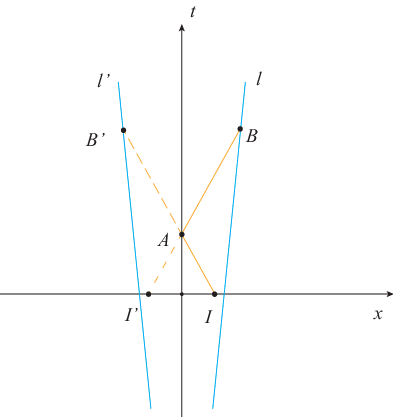
(a)

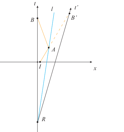
(a)

Figure 5: Transformation of a world line. For details, please see the main text of Appendix A.

After explaining the treatment in Eq. (15), we now continue to the understanding of Eq. (30). Similar to the mirror-symmetric operation in the laboratory reference frame, we could deal with the collision between the particle and the moving piston by carrying out a mirror-symmetric operation in the reference frame of the piston. After a Lorentz transformation back to the laboratory reference frame, the result is shown in Fig. 5(a). Points $I$,$A$,$B$ denote the initial state of the particle, a collision between the particle and the moving piston, and the next collision between the particle and the fixed boundary. $B^{\prime}$ is the auxiliary event of $B$. Just like the case in Fig. 4(a), in the reference frame of the moving piston, the auxiliary world line of the particle is a straight line. Therefore, after a Lorentz transformation the auxiliary world line of the particle is still a straight line $I-A-B^{\prime}$. The auxiliary world line of the fixed boundary is denoted as $t^{\prime}$. The velocity of $t^{\prime}$ is $2v_{p}/(1+v_{p}^{2})$, according to the Lorentz transformation. The intercept of the line $t^{\prime}$ can be determined as follows: the world line of the fixed boundary and moving piston intersect at point $R$ with space and time coordinate $(0,-L/v_{p})$. In the reference frame of the moving piston, the auxiliary world line of the fixed boundary and the moving piston intersect at the same point $R$. Therefore, in the laboratory reference frame, the auxiliary world line of the fixed boundary $t^{\prime}$ also passes through $R$, and the intercept of $t^{\prime}$ must be $-L/v_{p}$.

The mirror-symmetric operation transforms not only the world lines, but also the coordinate frames. In the reference frame of the fixed boundary, the $t$-axis is the world line of the boundary itself. After a coordinate transformation related to a collision with the moving piston, the auxiliary world line of the fixed boundary represents the auxiliary $t^{\prime}$-axis. The auxiliary $x^{\prime}$-axis should be orthogonal to $t^{\prime}$-axis, and the origin of coordinates (point $O$) should be transformed accordingly: $x$-axis and $l$ intersect at $P_{0}$, and thus $x^{\prime}$-axis also passes through $P_{0}$ (see Fig. 6(a). The intersection of the auxiliary $x^{\prime}$-axis and $t^{\prime}$-axis is the auxiliary origin $O^{\prime}$. If we denote the time coordinate of event $B$ in the coordinate frame $xOt$ as $t_{B}$ and the time coordinate of event $B^{\prime}$ in the coordinate frame $x^{\prime}O^{\prime}t^{\prime}$ as $t^{\prime}_{B^{\prime}}$, then, as a result of such coordinate transformation, $t^{\prime}_{B^{\prime}}=t_{B}$. The method that we evaluate the time coordinate of a real event with the help of an auxiliary event is still valid when dealing with the collision with the moving piston.

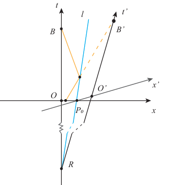
(a)

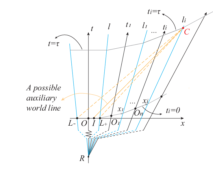
(b)

Figure 6: Transformation of the coordinate frame and the complete world line. For details, please see the main text of Appendix A.

By performing the coordinate transformation repeatedly, we could figure out the complete auxiliary world line of the particle and every auxiliary coordinate frame. The possible space-time region is $S_{0}=\{(x,t)|0\leq t\leq\tau,0\leq x\leq L+v_{p}t\}$, and the auxiliary regions can be determined accordingly: each gray line segment represents $t_{i}=0$ or $t_{i}=\tau$, $t_{i}$ is the time coordinate of an auxiliary event in the $i$-th auxiliary coordinate frame. In Fig. 6(b), regions between gray line segments are possible auxiliary regions. The red dot $C$ represents the event that a particle happens to collide exactly $i+1$ times when $t=\tau$. The position and time coordinate of C in the initial coordinate frame $xOt$ is denoted as $(x_{C},t_{C})$. Every auxiliary world line $IC$ with the initial condition $I(x_{I},v_{I})$ that passes through $C$ satisfies the critical condition

$$x_{I}=x_{C}-v_{I}\cdot t_{C}$$ (46)

which is the same as Eq. (30) when $n=i+1$. Such world lines lie between the two orange dashed lines $L_{-}C$ and $L_{+}C$ where $L_{-}$ and $L_{+}$ denote the particles with the initial position $-L$ and $L$. It is clear that the initial positions and velocities of auxiliary world lines satisfy a linear relation if every world line passes through a fixed point $C$, which explains the pictorial intuition mentioned above.

Appendix B Details of the Integration

Here we explain the computational details of deriving Eq. (27) from Eq. (26) and give a pictorial explanation for the overlap factor $\varphi_{n}.$ The integration

$$P(W)=\int_{-1}^{1}\mathrm{d}x\int_{0}^{1}\mathrm{d}v\frac{e^{-\frac{\beta}{\sqrt{1-v^{2}}}}\delta(W-W_{\tau}(x,v))}{2K_{1}(\beta)(1-v^{2})^{\frac{3}{2}}}$$ (47)

can be separated into parts

$$P(W)=\sum_{n}\int_{D_{n}}\mathrm{d}x\mathrm{d}v\frac{e^{-\frac{\beta}{\sqrt{1-v^{2}}}}\delta(W-W_{\tau}(v))}{2K_{1}(\beta)(1-v^{2})^{\frac{3}{2}}},$$ (48)

where $D_{n}$ is the domain of integration for all the $(x,v)$ values that the particle collide $n$ times. Note that within each domain $D_{n},$ the trajectory work becomes independent of $x.$ Recall that those particles that collide exactly $n$ times lie in a straight line on the $x-v$ plane, with the equation

$$\xi_{n}(v)=-T_{n}v+X_{n},$$ (49)

where

$$T_{n}=\frac{\alpha_{p}^{-(n-1)}-1-\alpha_{p}+\alpha_{p}^{n}}{1-\alpha_{p}}+\frac{\alpha_{p}^{-(n-1)}+\alpha_{p}^{n}}{1+\alpha_{p}}\cdot\tau$$ (50)

and

$$X_{n}=\frac{\alpha_{p}^{-(n-1)}-\alpha_{p}^{n}}{1-\alpha_{p}}+\frac{\alpha_{p}^{-(n-1)}-\alpha_{p}^{n}}{1+\alpha_{p}}\cdot\tau$$ (51)

are the slopes and the intercepts of the lines respectively. The separation of the domain of the integration is depicted in Fig. 7.

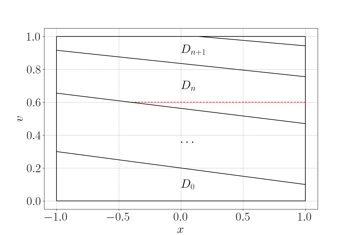
Figure 7: Dividing the domain of integration into parts and meaning of the overlap factor, where the length of the red dashed line is the value of $\varphi_{n}$ at the same $v$

We see that, since in each part the integrand is independent of $x$, we can integrate it out first, giving rise to

$$\begin{split}&\int_{D_{n}}\mathrm{d}x\mathrm{d}v\frac{e^{-\frac{\beta}{\sqrt{1-v^{2}}}}\delta(W-W_{\tau}(v))}{2K_{1}(\beta)(1-v^{2})^{\frac{3}{2}}}\\ &=\int\mathrm{d}v\frac{e^{-\frac{\beta}{\sqrt{1-v^{2}}}}\delta(W-W_{\tau}(v))}{2K_{1}(\beta)(1-v^{2})^{\frac{3}{2}}}\varphi_{n}(v),\end{split}$$ (52)

where the value of $\varphi_{n}(v)$ is the length of the line segment shown in Fig. 7. With the equation of all the lines known, we can compute the overlap factor as Eq. (28).

What is left involves integrating a Dirac $\delta$ function, we have

$$\begin{split}&\int\mathrm{d}v\frac{e^{-\frac{\beta}{\sqrt{1-v^{2}}}}\delta(W-W_{\tau}(v))}{2K_{1}(\beta)(1-v^{2})^{\frac{3}{2}}}\varphi_{n}(v)\\ &=\left.\frac{e^{-\frac{\beta}{\sqrt{1-v^{2}}}}}{2K_{1}(\beta)(1-v^{2})^{\frac{3}{2}}}\varphi_{n}(v)\left(\frac{\mathrm{d}W_{\tau}}{\mathrm{d}v}\right)^{-1}\right|_{W_{\tau}(v)=W}\\ &=\varphi_{n}(v_{n}(W))\frac{e^{-\frac{\beta}{\sqrt{1-v_{n}(W)^{2}}}}}{(\alpha_{p}^{-n}-1)\left[1+\alpha_{p}^{n}-v_{n}(W)(1-\alpha_{p}^{n})\right]}.\end{split}$$ (53)

The $n=0$ case should be treated separately. This is because all particles that can not catch up with the piston contribute to the probability at $W=0,$ resulting in a $\delta$ peak with the amplitude

$$P_{0}=\int_{0}^{1}\mathrm{d}v\frac{\varphi(v)e^{-\frac{\beta}{\sqrt{1-v^{2}}}}}{2K_{1}(\beta)(1-v^{2})^{\frac{3}{2}}}.$$ (54)

Summing up all the pieces at hand we have the result Eq. (27).

References

- Jarzynski [1997] C. Jarzynski, Nonequilibrium equality for free energy differences, Phys. Rev. Lett. 78, 2690 (1997).
- Nolte and Engel [2009] R. Nolte and A. Engel, Jarzynski equation for the expansion of a relativistic gas and black-body radiation, Physica A: Statistical Mechanics and its Applications 388, 3752 (2009).
- Lua and Grosberg [2005] R. C. Lua and A. Y. Grosberg, Practical applicability of the jarzynski relation in statistical mechanics: A pedagogical example, J. Phys. Chem. B 109, 6805 (2005).
- Quan and Jarzynski [2012] H. T. Quan and C. Jarzynski, Validity of nonequilibrium work relations for the rapidly expanding quantum piston, Phys. Rev. E 85, 031102 (2012).
- Gong et al. [2014] Z. Gong, S. Deffner, and H. T. Quan, Interference of identical particles and the quantum work distribution, Phys. Rev. E 90, 062121 (2014).
- Goldstein [1980] H. Goldstein, Classical Mechanics (Addison-Wesley, 1980).
- Jüttner [1911] F. Jüttner, Das Maxwellsche Gesetz der Geschwindigkeitsverteilung in der Relativtheorie, Annalen der Physik 339, 856 (1911).
- Pathria [1972] R. K. Pathria, Statistical mechanics. (1972).
- Gong et al. [2016] Z. Gong, Y. Lan, and H. T. Quan, Stochastic thermodynamics of a particle in a box, Phys. Rev. Lett. 117, 180603 (2016).
- Jarzynski [2006] C. Jarzynski, Rare events and the convergence of exponentially averaged work values, Phys. Rev. E 73, 046105 (2006).