Generally covariant geometric momentum and geometric potential for a Dirac fermion on a two-dimensional hypersurface
Abstract
Geometric momentum is the proper momentum for a moving particle constrained on a curved surface, which depends on the outer curvature and has observable effects. In the context of multi-component quantum states, geometric momentum should be rewritten as generally covariant geometric momentum. For a Dirac fermion constrained on a two-dimensional hypersurface, we give the generally covariant geometric momentum, and show that on the pseudosphere and the helical surface there exist no curvature-induced geometric potentials. These results verify that the dynamical quantization conditions are effective in dealing with constrained systems on hypersurfaces, and one could obtain the generally convariant geometric momentum and the geometric potential of a spin particle constrained on surfaces with definite parametric equations.
I Introduction
The quantum motion constrained on a two-dimensional curved surface is a unavoidable practical topic with the advance of quantum technologies, ranging from quantum physics to condensed matter physics. Typical examples include the spectrum of polyatomic molecules [1], the electronic states on helicoidal and Beltrami surfaces [2, 3, 4], the curvature-induced change of the electronic spectrum in graphene nanoribbons [5, 6], and the geometry-induced quantum spin Hall effect [7]. The classical Hamiltonian is known to be composed of the intrinsic coordinate and momentum, and the motion of a free particle that moves nonrelativistically on the surface only depends on its intrinsic geometry. The form of the equation of motion with denoting the Poisson bracket for an observable remains the same in quantum mechanics , which is the origin of fundamental quantum conditions [8]. This is a consequence of the Dirac’s canonical quantization, by which one can directly construct the quantum operators.
The fundamental quantum conditions refer to a set of commutations between the components of coordinate and momentum operators, writing
| (1) |
Here, and stands, respectively, for the coordinate operator and momentum operator of a particle moving in -dimensional Euclidean space . However, it is not the case once the system is constrained. For a particle that is constrained to remain on a smooth curved surface in , the Poisson bracket must be replaced by the Dirac bracket in canonical quantization procedures, leading to the quantum conditions [9, 10]
| (2) |
where represents a suitable construction of the Hermitian operator of an observable . The hypersurface can be described by a constraint in the configurational space as and the equation of the surface is chosen as , such that the normal vector is . As a consequence, only the unit normal vector and/or its derivatives enter the physics equation regardless of the surface equation [11, 12].
Within the above quantum conditions, there are many forms of the quantum momentum because of the operator-ordering problem in , leading to the fact that even the proper form of the momentum and the Hamiltonian cannot be determined unless more conditions are presented [13, 14, 15, 16]. But we do not concern with the Hamiltonian in the present work. Taking the symmetry as a fundamental priority in quantization procedures, we attempt to construct more commutation relations like and so as to simultaneously quantize the Hamiltonian together with coordinates and momenta, rather than to replace the coordinate and momentum operators into some presumed forms of Hamiltonian. In order to go beyond the operator-ordering problem, we have the dynamical quantization conditions as [17]
| (3) | |||||
| (4) |
where is the mass of the particle, and Eq. (4) indicates that the particle experiences no tangential force. The fundamental quantization conditions and the dynamical quantization conditions constitute the so called enlarged canonical quantization scheme, which gives the explicit form of the momentum as [18, 19, 20]
| (5) |
where is the gradient operator on the surface with being the usual gradient operator in and denoting the mean curvature, in which hereafter repeated indices are summed over and that is in fact the trace of the extrinsic curvature tensor. We call the geometric momentum for its dependence on the geometric invariants. This momentum satisfies the following simplest form of commutation
| (6) |
and the compatibility of constraint condition , which means that in quantum mechanics the motion lies in the tangential plane and corresponds to the constrained condition in classical mechanics: [18, 19, 20]. Geometric momentum depends on the extrinsic geometry of the embedding of in , and is purely quantum mechanical. The extrinsic geometry highlights a fundamental difference between confinements in classical and quantum physics. Note that the geometric momentum had been experimentally verified [21], indicating that quantum mechanics based on purely intrinsic geometry does not offer a proper description of the constrained motions, unless the extrinsic examination is performed as well.
The geometric momentum is sufficient for a quantum state of single component. When one considers the multi-component quantum states [22, 23], however, the gauge structure should be also included. With the gradient operator and a transformation , we immediately have the generally covariant geometric momentum [24]
| (7) |
where denotes the gauge potential with , the spin connection, and the Dirac spin matrix [23]. One can rewrite the as the product of and , and take the eigenvalues of the matrix as the effective interaction strength. The generally covariant geometric momentum in this form is applicable to both relativistic and nonrelativistic particles regardless of the mass.
The celebrated curvature-induced geometric potential has also been experimentally confirmed [25, 26], and hence the existence of the geometric potential for the motion on a curved surface is indispensable and worthy of investigation. For a Dirac fermion that is constrained typically on a two-dimensional curved surface of revolution, such as torus, catenoid and symmetric ellipsoid, there is no existence of the geometric potential [27]. A natural question thus arises as to whether this feature is universal within two-dimensional hypersurfaces. We demonstrate, in the present work, the formalism of obtaining the geometric potential on a hypersurface, and show that for the case of a two-dimensional pseudosphere and a helical surface it is a constant matrix independent of the parameters, which is composed of the -direction Pauli matrix and the identity matrix. There is currently not a general result for a constrained Dirac fermion on two-dimensional hypersurfaces. The clear framework, however, facilitates the access to both the generally covariant geometric momentum and the geometric potential for the surfaces with definite parametric equations.
The rest of the paper is organized as follows. In Sec. II, we give the generally covariant geometric momentum and the geometric potential, respectively, for a Dirac fermion that is constrained on a curved surface with a formal parametric equation. In Sec. III we present two typical cases with a two-dimensional pseudosphere and a helical surface as comparisons. We conclude our results in Sec. IV.
II Generally covariant geometric momentum and geometric potential on a curved surface
To be specific, we consider a Dirac fermion that is constrained to move on a curved surface with a formal parametric equation , where can be the functions of either or . According to the definiton of generally covariant geometric momentum, we first calculate the natural basis of the curved surface by and , and the unit normal vector is expressed as , which leads to the metric . One can subsequently obtain the inverse component of the natural frame , and the fundamental form of the curved surface is , with and being the relative components of the dreibeins, resulting in the transfer matrix between the space orthogonal coordinates and the local coordinates of the curved surface. The covariant differentiation on a curved surface is , and the gradient operator on a curved surface is denoted by . The gauge part can be denoted as , we thus obtain the respective components of the generally covarient geometric momentum
| (8) | |||||
| (9) | |||||
| (10) |
where is the geometric momentum of the particle without spin.
For a fermion on a two-dimensional surface, the covariant Dirac equation can be generally written as
| (11) |
with representing the reduced mass of the particle, and the Hamiltonian is . We suppose that the geometric potential is a general matrix
| (12) |
where are functions of and , and hence the Hamiltonian including the geometric potential is
| (13) |
and one can resolve the problem of whether there exists geometric potential in relativistic Hamiltonian, by respectively calculating the commutations of three components with
| (14) |
Finally, we consider the quantization conditions
| (15) |
according to which one obtains the situation for that the dynamic quantization conditions are met. We should, at this point, reach the explicit results for a Dirac fermion constrained on a two-dimensional hypersurface.
III A Dirac fermion on a pseudosphere and a helical surface
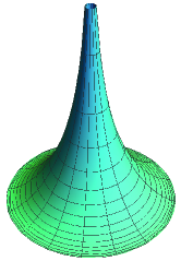
We are now in position to take two typical cases into account according to the above formalism, and verify that whether the enlarged canonical quantization scheme is effective in dealing with constrained systems in curved surfaces. For a two-dimensional pseudosphere, its parametric equation can be
| (16) |
where , and is a constant, as depicted in Fig. 1. According to the natural basis and the relative components of the dreibeins, the non-zero term spin connection is
| (17) |
and the gauge parts of the gradient operator are
| (18) | |||||
| (19) |
In addition, the mean curvature of the pseudosphere is , leading to the components of the generally covariant geometric momentum, respectively,
| (20) | |||||
where
| (21) | |||||
| (22) | |||||
| (23) |
The contravariant component of Dirac spin matrix under local coordinate is
| (26) |
and the Hamiltonian can be rewritten as
| (27) |
After some computations, we reach the three equations for the geometric potential
| (28) | |||||
| (29) | |||||
| (30) |
It is obvious that only when , with and being constant, the dynamic quantization condition is met. Thus the geometric potential for a Dirac fermion constrained on a pseudosphere is
| (31) |
which is a constant matrix composed of the -direction Pauli matrix and the identity matrix. According to Ref. [27] involving two-dimensional curved surface of revolution, one can choose and as zero by shifting the reference point of the energy, which indicates that there is no existence of the geometric potential, i.e., , and hence the expression of the Hamiltonian is reasonable.
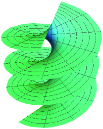
With respect to the other example, in the three-dimensional flat space the parametric equation for a helical surface under cartesian coordinate is
| (32) |
with , and , as sketched in Fig 2. The mean curvature , and one can follow the same lines as in the case of pseudosphere to obtain the explicit expressions of the generally covariant geometric momentum of the helical surface
| (33) | |||||
with
| (34) | |||||
| (35) | |||||
| (36) |
The contravariant component of Dirac spin matrix under local coordinate is
| (39) |
resulting in the rewritten Hamiltonian
| (40) |
The corresponding geometric potential are also straightforward
| (41) | |||||
| (42) | |||||
| (43) |
The general solutions of the above equations are , where and are constant, and the geometric potential for a Dirac fermion confined on a helical surface is straightforward
| (44) |
which also indicates no existence of the geometric potential. The helical surface is not really a curved surface of revolution, while the outcome happens to be similar to that of the pseudosphere. If one chooses other hypersurfaces, the features would probably vary, and offer insights into practical explorations.
IV Conclusions and Discussions
The fundamental and dynamical quantization conditions based on the quantization scheme of the classical system are available for dealing with a particle that is constrained to move relativistically on a curved surface. We obtain the generally covariant geometric momentum of a Dirac fermion constrained on a two-dimensional hypersurface, and demonstrate that there exist no geoemtric potential for the Dirac fermion constrained on both a pseudosphere and a helical surface. They are constant matrices independent of the parameters, and can be composed of the -direction Pauli matrix and the identity matrix.
Although we are currently not able to figure out the general results for a Dirac fermion constrained on a two-dimensional hypersurface, it is convenient to resolve the curved system with explicit parametric equations based on the theoretical framework. For other spin particles constrained on a hypersurface, the corresponding properties remain interesting open questions, and are worthy of further studies.
Acknowledgments
We thank Professor Quan-Hui Liu for the helpful discussions. This work was supported by the Natural Science Foundation of Sichuan Province (Grant No. 2023NSFSC1330) and the Natural Science Research Start-up Foundation of Recruiting Talents of Nanjing University of Posts and Telecommunications (Grant No. NY223065).
References
- [1] P. Maraner, Monopole gauge fields and quantum potentials induced by the geometry in simple dynamical systems, Ann. Phys. (NY) 246, 325 (1996).
- [2] B. Jensen, Electronic states on the helicoidal surface, Phys. Rev. A 80, 022101 (2009).
- [3] V. Atanasov, R. Dandoloff, and A. Saxena, Geometry-induced charge separation on a helicoidal ribbon, Phys. Rev. B 79, 033404 (2009).
- [4] J. Furtado, Electronic states in a quantum Beltrami surface, Phys. Lett. A 483, 129065 (2023).
- [5] M. B. Belonenko, N. G. Lebedev, N. N. Yanyushkina, A. V. Zhukov, and M. Paliy, Electronic spectrum and tunneling current in curved graphene nanoribbons, Solid State Commun. 151, 1147 (2011).
- [6] A. V. Zhukov, R. Bouffanais, N. N. Konobeeva, and M. B. Belonenko, On the electronic spectrum in curved graphene nanoribbons, JETP Lett. 97, 400 (2013).
- [7] Y. L. Wang, H. Zhao, H. Jiang, H. Liu, and Y. F. Chen, Geometry-induced monopole magnetic field and quantum spin Hall effects, Phys. Rev. B 106, 235403 (2022).
- [8] P. A. M. Dirac, The fundamental equations of quantum mechanics, Proc. R. Soc. London, Ser. A 109, 642 (1925).
- [9] T. Homma, T. Inamoto, and T. Miyazaki, Schrödinger equation for the nonrelativistic particle constrained on a hypersurface in a curved space, Phys. Rev. D 42, 2049 (1990).
- [10] J. R. Klauder and S.V. Shabanov, Coordinate-free quantization of second-class constraints, Nucl. Phys. B 511, 713 (1998).
- [11] Z. Li, L. Q. Lai, Y. Zhong, and Q. H. Liu, The curvature-induced gauge potential and the geometric momentum for a particle on a hypersphere, Ann. Phys. (NY) 432, 168566 (2021).
- [12] Z. Li, X. Yang, and Q. H. Liu, Curvature-induced noncommutativity of two different components of momentum for a particle on a hypersurface, Commun. Theor. Phys. 73, 025104 (2021).
- [13] M. Ikegami, Y. Nagaoka, S. Takagi, and T. Tanzawa, Quantum mechanics of a particle on a curved surface, Prog. Theor. Phys. 88, 229 (1992).
- [14] N. Ogawa, K. Fujii, and A. Kobushukin, Quantum mechanics in Riemannian manifold, Prog. Theor. Phys. 83, 894 (1990).
- [15] N. Ogawa, K. Fujii, N. Chepilko, and A. Kobushkin, Quantum mechanics in Riemannian manifold. II, Prog. Theor. Phys. 85, 1189 (1991).
- [16] N. Ogawa, The difference of effective Hamiltonian in two methods in quantum mechanics on submanifold, Prog. Theor. Phys. 87, 513 (1992).
- [17] D. K. Lian, L. D. Hu, and Q. H. Liu, Geometric potential and Dirac quantization, Ann. Phys. (Berlin) 530, 1700415 (2018).
- [18] Q. H. Liu, L. H. Tang, and D. M. Xun, Geometric momentum: The proper momentum for a free particle on a two-dimesional sphere, Phys. Rev. A 84, 042101 (2011).
- [19] Q. H. Liu, Geometric momentum and a probe of embedding effects, J. Phys. Soc. Jpn. 82, 104002 (2013).
- [20] Q. H. Liu, Geometric momentum for a particle constrained on a curved hypersurface, J. Math. Phys. 54, 122113 (2013).
- [21] R. Spittel, P. Uebel, H. Bartelt, and M. A. Schmidt, Curvature-induced geometric momenta: the origin of waveguide dispersion of surface plasmons on metallic wires, Opt. Express 23, 12174 (2015).
- [22] D.-H. Lee, Surface states of topological insulators: the Dirac fermion in curved two-dimensional spaces. Phys. Rev. Lett. 103, 196804 (2009).
- [23] A. Iorio and G. Lambiase, Quantum field theory in curved graphene spacetimes, Lobachevsky geometry, Weyl symmetry, Hawking effect, and all that, Phys. Rev. D 90, 025006 (2014).
- [24] Q. H. Liu, Z. Li, X. Y. Zhou, Z. Q. Yang, and W. K. Du, Generally covariant geometric momentum, gauge potential and a Dirac fermion on a two-dimensional sphere, Eur. Phys. J. C 79, 712 (2019).
- [25] A. Szameit, F. Dreisow, M. Heinrich, R. Keil, S. Nolte, A. Tünnermann, and S. Longhi, Geometric potential and transport in photonic topological crystals, Phys. Rev. Lett. 104, 150403 (2010).
- [26] J. Onoe, T. Ito, H. Shima, H. Yoshioka, S. Kimura, Observation of Riemannian geometric effects on electronic states, Europhys. Lett. 98, 27001 (2012).
- [27] Z. Q. Yang, X. Y. Zhou, Z. Li, W. K. Du, and Q. H. Liu, No existence of the geometric potential for a Dirac fermion on a two-dimensional curved surface of revolution, Phys. Lett. A 384, 126604 (2020).