On Merton’s Optimal Portfolio Problem
under Sporadic Bankruptcy

Abstract.

Consider a stock market following a geometric Brownian motion and a riskless asset continuously compounded at a constant rate. Assuming the stock can go bankrupt, i.e., lose all of its value, at some exogenous random time (independent of the stock price) modeled as the first arrival time of a homogeneous Poisson process, we study the Merton’s optimal portfolio problem consisting of maximizing the expected logarithmic utility of the total wealth at a preselected finite maturity time. First, we present a heuristic derivation based on a new type of Hamilton-Jacobi-Bellman equation. Then, we formally reduce the problem to a classical controlled Markovian diffusion with a new type of terminal and running costs. A new version of Merton’s ratio is rigorously derived using Bellman’s dynamic programming principle and validated with a suitable type of verification theorem. A real-world example comparing the latter ratio to the classical Merton’s ratio is given.
Keywords: Merton’s portfolio problem; Markov-switching processes; absorbing processes; Hamilton-Jacobi-Bellman equation; logarithmic utility.

1. Introduction

In this paper, we investigate the dynamic optimal allocation problem in a situation where security prices are subject to exogenous events like bankruptcy. The optimal portfolio problem was first considered by R. Merton [25] for multiple stocks that follow a multi-dimensional geometric Brownian motion [27]. For a single stock, the price $S_{t}$ at time $t$ is modeled as a Markovian diffusion process that solves the stochastic differential equation

(1) $$\mathrm{d}S_{t}=\mu S_{t}\mathrm{d}t+\sigma S_{t}\mathrm{d}B_{t}$$

with a standard Wiener process $(B_{t})_{t\geq 0}$, while the risk-free asset follows the ordinary differential equation

(2) $$\mathrm{d}R_{t}=rR_{t}$$

with a constant risk-free rate $r$. Assuming an isoelastic utility function

(3) $$U(W)=\begin{cases}\frac{W^{1-\gamma}-1}{1-\gamma},&\gamma\geq 0,\\ \log(W),&\gamma=1\end{cases}$$

for some $\gamma\geq 0$, he derived [25] his, now classical, Merton ratio $\pi$ of the wealth to invest in stock

(4) $$\pi=\frac{\mu-r}{\gamma\sigma^{2}},$$

while the remaining fraction, $(1-\pi)$, of investor’s wealth at each time $t$ is invested in the risk-free asset.

The theoretical importance of Merton ratio is that it gives investors a simple and easily interpretable, yet rigorous rule how to allocate capital into the risky asset as to maximize the expected utility. The practical importance of this ratio is highlighted in a recent The Economist article [30]. We note that a similar formula exists that provides a guideline how to invest in multiple stocks. Indeed, assume the price vector $\boldsymbol{S}_{t}=(S_{t}^{1},S_{t}^{2},\dots,S_{t}^{p})^{T}$ of $p$ stocks follows a multivariate geometric Brownian motion

(5) $$\mathrm{d}\boldsymbol{S}_{t}=\operatorname{diag}(\boldsymbol{S})\big{(}\boldsymbol{\mu}\,\mathrm{d}t+\boldsymbol{\Sigma}^{1/2}\mathrm{d}\boldsymbol{B}_{t}\big{)}$$

with a $p$-variate standard Brownian motion $(\boldsymbol{B}_{t})_{t\geq 0}$, where $\boldsymbol{\mu}\in\mathbb{R}^{p}$ is the vector of expected returns and $\boldsymbol{\Sigma}\in\mathbb{R}^{p\times p}$ is a symmetric, positive definite covariance matrix between the $p$-variate innovations. According to [25], the optimal weights $\boldsymbol{\pi}=(\pi^{1},\pi^{2},\dots,\pi^{p})^{T}$ are given by

(6) $$\boldsymbol{\pi}=\frac{1}{\gamma}\boldsymbol{\Sigma}^{-1}\big{(}\boldsymbol{\mu}-r\mathds{1}_{p}\big{)}\text{ with }\mathds{1}_{p}=(1,1,\dots,1)\in\mathbb{R}^{p}.$$

Since the groundbreaking work of Merton [25], many authors investigated various variants of Merton optimal portfolio problem. For example, Wachter [31] considered the optimal portfolio problem for risky assets following a mean reverting processes and obtained an exact solution for the optimal allocation when markets are complete. Merton himself [26] applied his dynamic portfolio optimization approach to extend the usual capital asset pricing model (CAPM) to an in-temporal CAPM. The latter generalizes the usual CAPM model developed by Sharpe based on Markowitz portfolio problem. Efforts to incorporate other types of risky assets (such as fixed income securities) have been attempted as well. For instance, Brennan et al. [6] considered a Merton-type problem for fixed income securities and stocks but without any bankruptcy assumptions on the bonds. Karatzas et al. [16] considered the optimal portfolio problem for a general utility function and incorporated bankruptcy events. The bankruptcy event considered in the latter paper was not modeled as an exogenous event but was rather assumed to arise from the self-exciting (autoregressive) dynamics, i.e., the authors asked the question when it will be optimal for the security to default given an infinite time horizon and solved this problem of optimal bankruptcy. For applications in corporate finance, see [21] and [22].

The goal of this paper is to revisit Merton’s original problem and investigate the optimal allocation between stock and cash as to optimize the expected logarithmic utility at a finite maturity $T$ assuming, however, the stock can sporadically jump into bankruptcy at an exogenous random time $\tau\sim\mathrm{Exp}(\lambda)$, independent of the stock price, which is modeled as an exponential random variable with some parameter $\lambda>0$ corresponding to default intensity. The amended price dynamics reads then as

(7) $$\mathrm{d}S_{t}=\left\{\begin{array}[]{cl}\mu S_{t-}\mathrm{d}t+\sigma S_{t-}\mathrm{d}B_{t}&\text{for }t<\tau\\ 0\,\mathrm{d}t,&\text{for }t>\tau\end{array}\right.\text{ and }\Delta S_{\tau}=-S_{\tau-}$$

with the jump operator (viz. [23, Equation (1)])

(8) $$\Delta S_{t}:=S_{t}-S_{t-}$$

where $(B_{t})_{t\geq 0}$ is a standard Wiener process. The process in Equation (7) is a special two-state case of a more general Markov-switching jump diffusion process considered in [4, 32]. Indeed, the random bankruptcy time $\tau$ can be viewed as the first arrival time of a Poisson process or the jump time of a two-state continuous time Markov process with two states: pre-bankruptcy and post-bankruptcy, where the latter state is absorbing. The average time to bankruptcy $\mathbb{E}[\tau]$ is $\frac{1}{\lambda}$, while the conditional probability of banktruptcy is memoryless

(9) $$\mathbb{P}\big{\{}t\leq\tau<t+\Delta t\,|\,\tau\geq t\big{\}}=\lambda\Delta t+o(\Delta t)\text{ as }\Delta t\searrow 0\text{ for any }t\geq 0$$

as it is known to be the case for Poisson processes. A stochastic dynamics similar to Equation (7), albeit with non-random jump times, has recently been studied in [23]. Assuming the logarithmic utility function in this paper, we obtain the Merton ratio

(10) $$\pi_{t}=\left\{\begin{array}[]{cl}\frac{\mu-r+\sigma^{2}-\sqrt{\left(\sigma^{2}-(\mu-r)\right)^{2}+4\lambda\sigma^{2}}}{2\sigma^{2}},&t<\tau,\\ 0,&t\geq 0.\end{array}\right.$$

The expression in Equation (10) is reminiscent of the multivariate optimal allocation vector obtained in [1] in the context of portfolio choice in markets with contagion.

To some extent, our work has connection to portfolio optimization under Brownian motion perturbed with jump processes. For example, [9] investigated optimal portfolios under Levý innovations. Their optimization approach followed the classical Markowitz paradigm of mean variance. The authors adopted a framework of risk constraints, which is related to our problem as we consider stocks that have a risk of sporadic bankruptcy. An important distinction that jumps under a Levý process have an emerging property while stocks (contrary to bonds) do not emerge from bankruptcy.

A dynamic portfolio optimization problem for a stochastic model with jumps was considered in [10]. Like other works, the processes adopted were emerging processes with regime switching regulated by a Markov control process, which is separate from our case where the process enters an absorbing state. Another significant work in this direction is [1], in which the authors consider asset allocation when the stock follows a geometric Brownian motion and a jump process. Even though the stochastic processes considered are complicated, the authors were able to obtain an exact solution to the Merton allocation problem for logarithmic utility.

The optimization problem we consider in this work is inspired by similar problems on the bond side. To the best of our knowledge, this type of problem was first studied in [5]. The problem considered there was an optimization for stock cash and a bond with some default probability. The authors formulated the underlying optimization problem and presented a solution but omitted the final derivation of the Hamilton-Jacobi-Bellman (HJB) equation or a stochastic integral approach we employ in our paper. The problem was fully solved in [7, 8], where an optimal allocation problem for a bond with bankruptcy and a stock was considered. The authors set up an HJB equation with two regimes: the post-default and the pre-default regime. Our problem is separate from this scenario due to the fact that we consider stocks with exogenous bankruptcy occurrence. To the best of our knownledge, this type of problems with exogenous bankruptcies for stocks have not been previously considered. Our solution presented in Equation (10) is interesting on its own account as it mandates that one should never allocates the complete amount of investment into a stock with with positive bankruptcy probability or borrow money to invest in such stocks. It is also worthwhile to note that bankruptcy is an absorbing process and, as far as we know for optimal portfolios, such processes have not been considered before. The probability of bankruptcy can be significant for stocks with low credit quality and, thus, our solution is not a mere theoretical exercise but has a practically important bearing as we will show in the sequel. It should be reiterated that the process we consider is different from conventional models based on Poisson jump processes since the stock cannot recover from bankruptcy so that the latter is an absorbing state. On the other hand, we note that it is possible to consider similar models (cf. [4, 32]) that would incorporate semi-Markovian switching (viz. [24, Chapter 7]) between economic regimes that can be either absorbing or not absorbing. In this sense, our present work provides a blueprint for investigating optimal portfolio allocation problems for this type of models.

The rest of this paper is structured as follows. In Section 2, we introduce a probabilistic framework and state the problem. In Section 3, a simple heuristic calculation is presented to derive the Merton ratio from Equation (10). Without being rigorous, it is new and interesting on its own merit since it employs a non-conventional form of the Itô’s lemma to formally derive the optimality conditions following the idea originally presented in [19]. Similar to [4, 7], a pair of coupled HJB equations is derived to find the optimal weights. In Section 4, a rigorous solution to the optimal portfolio problem is obtained by reducing the expected terminal logarithmic utility objective for a stock with bankruptcy to a combination of exponentially weighted expected terminal and running logarithmic utilities without bankruptcy. The optimal Merton ratio (viz. Equation (10)) obtained with both approaches agree. In Section 5, we then illustrate our approach by compute the optimal allocation for a real-world stock with a non-trivial bankruptcy probability and confirm a material difference from the allocation produced with the usual Merton ratio. Summary and conclusions are given in Section 6. Proofs of auxiliary results are relegated to Appendix A.

2. Probabilistic Setup and Preliminaries

For time $t\geq 0$, let $S_{t}$ and $R_{t}$ denote the price of a defaultable stock following Equation (1) driven by a standard Brownian motion $(B_{t})_{t\geq 0}$ and and a riskfree asset satisfying Equation (2), where $\mu$, $\sigma>0$ and $r>0$ are the drift, volatility and risk-free rate, respectively. Assuming $W_{t}$ is the total wealth at time $t$ consisting of $\pi_{t}W_{t}$ dollars in stock and $(1-\pi_{t})X_{t}$ dollars in the riskless asset for some $\pi_{t}$, the dynamics of $X_{t}$ is given by equation

(11) $$\begin{split}\mathrm{d}W_{t}&=\left\{\begin{array}[]{cl}\big{(}\mu\pi_{t-}+r(1-\pi_{t-})\big{)}W_{t-}\mathrm{d}t+\sigma\pi_{t-}W_{t-}\mathrm{d}B_{t}&\text{for }0\leq t<\tau,\\ r(1-\pi_{t})W_{t}&\text{for }\tau\leq t\leq T,\end{array}\right.\\ \Delta W_{\tau}&=-\pi_{t}W_{\tau-},\\ W_{0}&=w\end{split}$$

where $w>0$ is a (given) initial wealth. Recall that $\tau\sim\mathrm{Exp}(\tau)$ is assumed stochastically independent of $(B_{t})_{t\geq 0}$. To emphasize the dependence of $W_{t}$ on $\pi_{t}$ and $\tau$, we will often write $W_{t}^{\pi,\tau}$.

To put Equation (11) into a formal framework similar to [23], consider the semi-Markov process

(12) $$\xi_{t}:=\mathds{1}_{\{t<\tau\}}$$

with the non-absorbing pre-default state $0$ and the absorbing post-default state $1$. Introducing the drift and volatility functions

(13) $$\begin{split}a(t,W,\pi,\xi)&=\big{(}\mu\pi+r(1-\pi)\big{)}(1-\xi)+(1-\pi)\xi,\\ b(t,W,\pi,\xi)&=\sigma\pi(1-\xi),\end{split}$$

Equation (11) can be expressed as

(14) $$\begin{split}\mathrm{d}W_{t}&=a(t-,W_{t-},\pi_{t-},\xi_{t-})\mathrm{d}t+b(t-,W_{t-},\pi_{t-},\xi_{t-})\mathrm{d}B_{t}\text{ for }0\leq t\leq T,\\ \Delta W_{\tau}&=-\pi_{\tau-}W_{\tau-}\text{ if }\tau\leq T,\\ W_{0}&=w.\end{split}$$

It should be emphasized that, unlike [23], the switching time in Equation (14) is random.

Consider the filtered probability space $(\Omega,(\mathcal{F}_{t})_{t\geq 0},\mathbb{P})$ with the minimal $\sigma$-algebra

(15) $$\mathcal{F}_{t}=\sigma(B_{t},\xi_{t})\text{ for }t\geq 0.$$

Arguing similar to [4], for any adapted process $(\pi_{t})_{t\geq 0}$ with

$$\int_{0}^{T}\pi_{t}^{2}\mathrm{d}t<\infty\;\mathbb{P}\text{-a.s.},$$

Equation (14) possesses a unique strong solution (being a cádlág process) denoted by $(W_{t}^{\pi,\tau})_{t\geq 0}$ on any time interval $[0,T]$. The set of admissible controls for Equation (14) can be defined as

(16) $$\begin{split}\mathcal{A}_{w}:=\big{\{}\pi\,|\,&(\pi)_{t\in[0,T]}\text{ is adapted with }\int_{0}^{T}\pi_{t}^{2}\mathrm{d}s<\infty\;\mathbb{P}\text{-a.s.},\\ &(W_{t})_{t\in[0,T]}\text{ is a unique strong solution such that }W_{0}^{\pi,\tau}=w,\\ &W_{t}^{\pi,\tau}(\omega)>0\;\mathbb{P}\otimes\nu\text{ a.e.~{}in }[0,T]\times\Omega,\;\mathbb{E}\big{[}\mathop{\operatorname{ess\,sup}}_{t\in[0,T]}U(W_{t}^{\pi,\tau})_{-}\big{]}<\infty\big{\}}\end{split}$$

where $x_{-}=\max\{0,-x\}$ denotes the negative part of $x$ and $\nu$ is the Borel measure on $[0,\infty)$.

Employing the logarithmic utility function

(17) $$U(W)=\log(W),$$

consider the terminal expected utility functional

(18) $$J(\pi)=\mathbb{E}_{\mathcal{F}_{T}}\big{[}U(W^{\pi,\tau}_{T})\big{]}.$$

Thus, the optimal portfolio problem reads as

(19) $$J(\pi)\to\min_{\pi\in\mathcal{A}_{w}},\quad\pi^{\ast}=\mathop{\operatorname{arg\,max}}_{\pi\in\mathcal{A}_{w}}J(W^{\pi,\tau},\pi),\quad W_{t}^{\ast}=W_{t}^{\pi^{\ast},\tau}.$$

To solve the optimal control problem, we first want to explicitly characterize the forward map $\pi\mapsto W^{\pi,\tau}$ mapping each admissible control $\pi\in\mathcal{A}_{w}$ to the unique strong solution $(W^{\pi,\tau}_{t})_{t\geq 0}$ of Equation (11). To this end, let $(X_{t})_{t\geq 0}$ denote the unique strong solution to the classical wealth SDE without bankruptcy

(20) $$\mathrm{d}X_{t}=\big{(}\mu\pi_{t}+r(1-\pi_{t})\big{)}X_{t}\mathrm{d}t+\sigma\pi_{t}X_{t}\mathrm{d}B_{t}\text{ for }t>0,\quad X_{0}=w$$

explicitly given [18, Chapter 4] via

(21) $$X_{t}=\Phi_{t}w-\sigma\int_{0}^{t}\Phi_{t}\Phi_{s}^{-1}\pi_{s}\mathrm{d}s$$

with

$$\Phi_{t}=\exp\Big{(}\int_{0}^{t}\Big{(}\big{(}\mu\pi_{s}+r(1-\pi_{s})\big{)}-\frac{1}{2}\sigma^{2}\pi_{s}^{2}\Big{)}\mathrm{d}s+\sigma\int_{0}^{t}\pi_{s}\mathrm{d}B_{s}\Big{)}.$$

With this notation, the wealth process $(W_{t})_{t\in[0,T]}$ solving Equation (11) can be expressed as

(22) $$W_{t}=X_{t}\mathds{1}_{\{t<\tau\}}+\exp\Big{(}\int_{\tau}^{t}r(1-\pi_{s})\mathrm{d}s\Big{)}(1-\pi_{\tau-})X_{\tau}\mathds{1}_{\{t\geq\tau\}}.$$

Indeed, if the bankruptcy has not happened at time $t$ or before, $W_{t}$ is same as $X_{t}$. Otherwise, all capital allocated in the stock at time $\tau-$ (viz. $\pi_{\tau-}X_{\tau-}$) will be lost, while the remaining capital allocated in the riskless asset (viz. $(1-\pi_{\tau-})X_{\tau-}$) will continue accruing from time $\tau$ to time $t$.

As can be seen from Equation (22), the positivity of $W_{t}>0$ $\mathbb{P}\otimes\nu$-a.e. required in the definition of $\mathcal{A}_{w}$ in Equation (23) necessitates that

$$\pi_{t}(\omega)<1\text{ for }\mathbb{P}\otimes\nu\text{ for a.e. }(t,\omega)\in\Omega\times[0,T].$$

Indeed, letting $I=\{t\in[0,T]\,|\,\pi_{t}\geq 1\}$, we obtain

$$\begin{split}\mathbb{P}\{W_{t}\leq 0\}&=\mathbb{P}\Big{\{}\exp\Big{(}\int_{\tau}^{t}r(1-\pi_{s})\mathrm{d}s\Big{)}(1-\pi_{\tau-})X_{\tau}\mathds{1}_{\{T\geq\tau\}}\leq 0\Big{\}}\\ &=\mathbb{P}\Big{\{}(1-\pi_{\tau-})X_{\tau}\mathds{1}_{\{\tau\in I\}}\leq 0\Big{\}}=\mathbb{P}\{\tau\in I\},\end{split}$$

where we used the fact that $X_{t}>0$ $\mathbb{P}$-a.s. for a.e. $t\in[0,T]$. The latter probability vanishes if and only if $\nu(I)=0$.

Thus, the admissible set in Equation (23) can be equivalently expressed as

(23) $$\begin{split}\mathcal{A}_{w}:=\big{\{}\pi\,|\,&(\pi)_{t\in[0,T]}\text{ is adapted with }\int_{0}^{T}\pi_{t}^{2}\mathrm{d}t<\infty\;\mathbb{P}\text{-a.s.},\;\pi_{t}(\omega)<1\;\mathbb{P}\otimes\nu\text{ a.e.~{}in }\Omega\times[0,T],\\ &(W_{t})_{t\in[0,T]}\text{ is a unique strong solution with }W_{0}^{\pi,\tau}=w,\;\mathbb{E}\big{[}\mathop{\operatorname{ess\,sup}}_{t\in[0,T]}U(W_{t}^{\pi,\tau})_{-}\big{]}<\infty\big{\}}\end{split}$$

Analyzing Equation (22), we easily observe that any wealth fraction $\pi_{t}$ invested into stock after bankruptcy (i.e., $t\geq\tau$) in lieu of the riskfree asset can only reduce the terminal wealth, $W_{T}$, and, thus, the expected utility $J(\cdot)$. Therefore, without loss of generality, we can assume $\pi_{t}=0$ for $t\geq\tau$ leading to state-switching controls

(24) $$\pi_{t}=\pi^{\ast}_{\mathrm{pre}}\mathds{1}_{\{t<\tau\}}+\pi^{\ast}_{\mathrm{post}}\mathds{1}_{\{t\geq\tau\}}=\left\{\begin{array}[]{cl}\pi_{\mathrm{pre},t},&t<\tau,\\ \pi_{\mathrm{post},t},&t\geq\tau\end{array}\right.\quad\text{ with }\pi_{\mathrm{post},t}\equiv 0.$$

This furnishes a simplified version of Equation (22) given by

(25) $$W_{t}=X_{t}\mathds{1}_{\{t<\tau\}}+e^{r(t-\tau)}(1-\pi_{\tau-})X_{\tau}\mathds{1}_{\{t\geq\tau\}}$$

without violating any admissibility conditions.

3. Heuristic Derivation

We begin with a heuristic calculation of the optimal allocation strategy. To this end, we define the admissible set

$$\begin{split}\mathcal{A}_{t,w}:=\big{\{}\pi\,|\,&(\pi)_{s\in[t,T]}\text{ is adapted with }\int_{t}^{T}\pi_{s}^{2}\mathrm{d}s<\infty\;\mathbb{P}\text{-a.s.},\;\pi_{s}(\omega)<1\text{ for }\mathbb{P}\otimes\nu\text{ a.e.~{}in }\Omega\times[t,T],\\ &(W_{s})_{s\in[t,T]}\text{ is a unique strong solution with }W_{t}^{\pi,\tau}=w,\;\mathbb{E}\big{[}\mathop{\operatorname{ess\,sup}}_{s\in[t,T]}U(W_{s}^{\pi,\tau})_{-}\big{]}<\infty\big{\}}\end{split}$$

where $(W_{s}^{\pi,\tau})_{s\in[t,T]}$ solves the jump SDE in Equation (11) over $[t,T]$. Further, consider the value function

(26) $$V(t,w)=\sup_{\pi\in\mathcal{A}_{t,w}}\mathbb{E}_{\mathcal{F}_{T}}\big{[}U(W^{\pi,\tau}_{T})\,|\,W_{t}^{\pi,\tau}=w\big{]}.$$

In spirit of [4], we also introduce two auxiliary “conditional” value functions

(27) $$\begin{split}V^{\mathrm{pre}}(t,w)&=\sup_{\pi\in\mathcal{A}_{t,w}}\mathbb{E}_{\mathcal{F}_{T}}\big{[}U(W^{\pi,\tau}_{T})\,|\,t<\tau\big{]},\\ V^{\mathrm{post}}(t,w)&=\sup_{\pi\in\mathcal{A}_{t,w}}\mathbb{E}_{\mathcal{F}_{T}}\big{[}U(W^{\pi,\tau}_{T})\,|\,t=\tau\big{]}=\mathbb{E}_{\mathcal{F}_{T}}\big{[}U(W^{\pi=0,\tau}_{T})\,|\,t=\tau\big{]}\end{split}$$

corresponding to the case no bankruptcy has occurred at time $t$ or before and the case the bankruptcy occurs at time $t$, respectively. It should be noted that this framework allows for default-specific optimal control processes $\pi_{t}$, i.e.,

Using the law of total probability, the total value function in Equation (26) can be expressed as

(28) $$\begin{split}V(t,w)&=V^{\mathrm{pre}}(t,w)\,\mathbb{P}\{\tau<t\}+V^{\mathrm{post}}(t,w)\,\mathbb{P}\{\tau\geq t\}\\ &=(1-e^{-\lambda t})V^{\mathrm{pre}}(t,w)+e^{-\lambda t}V^{\mathrm{post}}(t,w).\end{split}$$

Arguing similar to Equation (25), we can explicitly compute the “post” conditional value function via

(29) $$V^{\mathrm{post}}(t,w)=U\big{(}e^{r(T-t)}(1-\pi_{t-})w\big{)}=r(T-t)+\log(1-\pi_{t-})+\log(w),$$

recalling that $U(\cdot)$ is the logarithmic utility function (viz. Equation (17)).

As for the “pre” conditional value function, on the strength of Equation (9), the conditional probability of no crash occurring in $[t,t+\mathrm{d}t]$ assuming no crash has occurred until time $t$ is $(1-\lambda\mathrm{d}t)+o(\mathrm{d}t)$, while the conditional probability of crash is $\lambda\mathrm{d}t+o(\mathrm{d}t)$. Thus, using an argumentation similar to [4, Theorem 3.3], we can heuristically derive an infinitesimal recursive formula for $V^{\mathrm{pre}}(t,w)$ reading as

(30) $$\begin{split}\mathrm{d}V^{\mathrm{pre}}(t,w)&=(1-\lambda\mathrm{d}t)\mathrm{d}V^{\mathrm{pre}}(t,w)+\lambda\mathrm{d}t\big{(}V^{\mathrm{post}}(t,w)-V^{\mathrm{pre}}(t,w)\big{)}+o(\mathrm{d}t)\\ &=(1-\lambda\mathrm{d}t)\mathrm{d}V^{\mathrm{pre}}(t,w)+\lambda\mathrm{d}t\big{(}r(T-t)+\log(1-\pi_{t-})+\log(w)-V^{\mathrm{pre}}(t,w)\big{)}+o(\mathrm{d}t)\end{split}$$

Let $\pi_{t}\in\mathcal{A}_{t,w}$. For a wealth process $(W_{s}^{\pi,\tau})_{s\in[t,T]}$ solving the jump SDE in Equation (11) subject to the initial condition $W_{t}^{\pi,\tau}=w$, we evaluate the differential $\mathrm{d}V^{\mathrm{pre}}(s,W_{s})$ for $t\leq s\leq T$. According to Equation (20), the wealth process satisfies

(31) $$\begin{split}\mathrm{d}W_{s}&=W_{s}\left(\pi_{s}\mu\mathrm{d}s+\pi_{s}\sigma\mathrm{d}B_{s}+(1-\pi_{s})r\mathrm{d}s\right),\\ (\mathrm{d}W_{s})^{2}&=W_{s}^{2}\pi_{s}^{2}\sigma^{2}\mathrm{d}s.\end{split}$$

Assuming $V^{\mathrm{pre}}(\cdot)$ is a smooth function, Itô’s rule (cf. [4, Theorem 3.5]) furnishes

(32) $$\begin{split}\mathrm{d}V^{\mathrm{pre}}(t,w)&=\partial_{w}V^{\mathrm{pre}}(t,w)(w\left(\pi_{t}\mu\mathrm{d}t+(1-\pi_{t})r\mathrm{d}t\right)+\frac{1}{2}\partial_{w}^{2}V^{\mathrm{pre}}(t,w)w^{2}\pi_{t}^{2}\sigma^{2}\mathrm{d}t+\partial_{t}V^{\mathrm{pre}}(t,w)\mathrm{d}t\\ &+\lambda\mathrm{d}t\left(r(T-t)+\log(1-\pi_{t})+\log(w)-V^{\mathrm{pre}}(t,w)\right),\end{split}$$

where we assume the continuity of $\pi_{s}$ (and, therefore, that of $\pi_{\mathrm{pre},s}$) for $t\leq s<\tau$ implying $\pi_{s-}=\pi_{s}$. Dividing by $\mathrm{d}t$ and passing to the limit $\mathrm{d}t\to 0$, we obtain an HJM-type equation for the “pre” conditional value function

(33) $$\partial_{t}V^{\mathrm{pre}}+\mathcal{H}(t,V^{\mathrm{pre}},\pi_{t},\partial_{w}V^{\mathrm{pre}},\partial_{w}^{2}V^{\mathrm{pre}})=0$$

where

(34) $$\begin{split}\mathcal{H}(t,w,\pi,V^{\mathrm{pre}},\partial_{w}V^{\mathrm{pre}},\partial_{ww}V^{\mathrm{pre}})=\sup_{\pi_{t}<1}&\Big{(}\partial_{w}V^{\mathrm{pre}}(w\left(\pi_{t}\mu+(1-\pi_{t})r\right)+\tfrac{1}{2}\partial_{w}^{2}V^{\mathrm{pre}}w^{2}\pi_{t}^{2}\sigma^{2}\\ &+\lambda\left(r(T-t)+\log(1-\pi_{t})+\log(w)-V^{\mathrm{pre}}\right)\Big{)}.\end{split}$$

In contrast to the usual HJB equation, we can observe that our HJM operator $\mathcal{H}(\cdot)$ additionally depends on the derivatives of the value function but also the value function itself.

Using the ansatz

(35) $$V(t,w)=\log(w)+f(t),$$

the first-order Fermat optimality condition for $g(\cdot)$ reads as

(36) $$(\mu-r)-\pi_{t}\sigma^{2}-\frac{\lambda}{1-\pi_{t}}=0.$$

Recalling $\pi_{t}^{\ast}=0$ for $t\geq\tau$ (viz. Equation (24)), the optimal allocation (cf. Equation (10)) is given as:

$$\pi_{t}^{\ast}=\pi^{\ast}_{\mathrm{pre}}\mathds{1}_{\{t<\tau\}}$$

with

$$\pi_{\mathrm{pre}}^{\ast}=\frac{\mu-r+\sigma^{2}-\sqrt{\left(\sigma^{2}-(\mu-r)\right)^{2}+4\lambda\sigma^{2}}}{2\sigma^{2}}.$$

Plugging $\pi_{t}^{\ast}$ back into Equation (34), the latter can be explicitly solved using the ansatz from Equation (35) yielding the value function $V=V(t,x)$. One would naturally expect the latter to satisfy

$$\max_{\pi\in\mathcal{A}_{t,w}}J(\pi)=V(t,x)=J(\pi^{\ast}).$$

Unfortunately, the optimal control problem in Equation (34) is not directly covered by the verification theorem for Markov-switching SDEs established in [4]. While latter results can likely be extended to our situation, an simpler strategy to avoid laborious proofs and calculations is to transform the problem in Equation (34) to a conventional controlled Markovian diffusion and invoking one of several rigorous verification theorems known in the literature for this class of optimal control problems.

4. Reduction to Controlled Markovian Diffusion

In this section, we present an alternative derivation that reduces the non-conventional optimal control problem discussed in Section 2 to the classical case. For the sake of simplicity, with some abuse of notation, we will write $\pi_{t}$ to denote $\pi_{\mathrm{pre},t}$ for the most part of this section until Equation (45), where $\pi_{t}$ reclaims its original meaning (cf. Equation (24)).

Our approach is inspired by [17]. Assuming the conditions of Fubini & Tonelli’s theorem are satisfied, we can write

$$\mathbb{E}_{\mathbb{P}_{W}\otimes\mathbb{P}_{\tau}}\big{[}u(Y_{T}^{\pi})\big{]} =\mathbb{E}_{\mathbb{P}_{W}}\Big{[}\mathbb{E}_{\tau}\big{[}u(Y_{T}^{\pi})\big{]}\Big{]}=\mathbb{E}_{\mathbb{P}_{W}}\Big{[}\int_{0}^{\infty}u(Y_{T}^{\pi})\varphi(t)\mathrm{d}t\Big{]}$$

$$=\mathbb{E}_{\mathbb{P}_{W}}\Big{[}\int_{0}^{\infty}\Big{(}u(X_{T})\mathds{1}_{\{T<t\}}+u\big{(}e^{r(T-t)}(1-\pi_{t})X_{t}\big{)}\mathds{1}_{\{T\geq t\}}\Big{)}\varphi(t)\mathrm{d}t\Big{]}$$

$$=\mathbb{E}_{\mathbb{P}_{W}}\Big{[}\int_{T}^{\infty}u(X_{T})\varphi(t)\mathrm{d}t\Big{]}+\mathbb{E}_{\mathbb{P}_{W}}\Big{[}\int_{0}^{T}u\big{(}e^{r(T-t)}(1-\pi_{t})X_{t}\big{)}\varphi(t)\mathrm{d}t\Big{]}$$

$$=\mathbb{E}_{\mathbb{P}_{W}}\Big{[}\Big{(}\int_{T}^{\infty}\varphi(t)\mathrm{d}t\Big{)}u(X_{T})\Big{]}+\mathbb{E}_{\mathbb{P}_{W}}\Big{[}\int_{0}^{T}u\big{(}e^{r(T-t)}(1-\pi_{t})X_{t}\big{)}\varphi(t)\mathrm{d}t\Big{]}$$

$$=\mathbb{P}_{\mathbb{P}_{\tau}}\{\tau\geq T\}\mathbb{E}_{\mathbb{P}_{W}}\big{[}u(X_{T})\big{]}+\mathbb{E}_{\mathbb{P}_{W}}\Big{[}\int_{0}^{T}u\big{(}e^{r(T-t)}(1-\pi_{t})X_{t}\big{)}\varphi(t)\mathrm{d}t\Big{]}$$

where $\mathbb{P}_{\mathbb{P}_{\tau}}\{\tau\geq T\}=\int_{T}^{\infty}\varphi(t)\mathrm{d}t$ solely depends on $T$ with $\varphi(\cdot)$ denoting the probability density function of $\tau$. As before, we choose $u(x)=\log(x)$ to be the logarithmic utility and assume $\tau\sim\mathrm{Exp}(\lambda)$ is exponentially distributed with some known intensity $\lambda>0$, i.e., $\varphi(t)=\lambda\exp(-\lambda t)\mathds{1}_{\{t\geq 0\}}$. Then the expected utility can be further simplified as

(37) $$\begin{split}\mathbb{E}_{\mathbb{P}_{W}\otimes\mathbb{P}_{\tau}}\big{[}u(Y_{T}^{\pi})\big{]}&=\mathbb{E}_{\mathbb{P}_{W}}\Big{[}\int_{0}^{T}\lambda e^{-\lambda t}\log\big{(}(1-\pi_{t})X_{t}\big{)}\mathrm{d}t\Big{]}\\ &+\mathbb{E}_{\mathbb{P}_{W}}\big{[}e^{-\lambda T}\log(X_{T})\big{]}+r\lambda\int_{0}^{T}(T-t)e^{-\lambda t}\mathrm{d}t\\ &=\mathbb{E}_{\mathbb{P}_{W}}\Big{[}\int_{0}^{T}\lambda e^{-\lambda t}\log\big{(}(1-\pi_{t})X_{t}\big{)}\mathrm{d}t\Big{]}\\ &+\mathbb{E}_{\mathbb{P}_{W}}\Big{[}e^{-\lambda T}\log(X_{T})+r\Big{(}T-\frac{1-e^{-\lambda T}}{\lambda}\Big{)}\Big{]}\end{split}$$

where $\tau$ is completely eliminated from the latter equation.

Therefore, we were able to reduce the original control problem with sporadic bankruptcy in Equations (11), (17), (18) and (19) to a classical stochastic control problem in Equations (20) and (37) with running and terminal costs for wealth $W_{t}$ so that the usual Bellman’s principle for Markovian diffusions can now be applied. Throughout the rest of the section, we adopt the notation of [13, Chapter IV]. Note that maximization of expected utility is equivalently expressed as minimimization of negative utility within this framework. Thus, we seek to minimize the functional

(38) $$J(\pi)=\mathbb{E}\Big{[}-\int_{0}^{T}\lambda e^{-\lambda t}\log\big{(}(1-\pi_{t})X_{t}\big{)}\mathrm{d}t\Big{]}+\mathbb{E}\Big{[}-e^{-\lambda T}\log(X_{T})-r\Big{(}T-\frac{1-e^{-\lambda T}}{\lambda}\Big{)}\Big{]}.$$

Since the terminal cost function in Equation (38) cannot be continuously extended to $x=0$, classical results (viz. [12, 13]) cannot be directly applied to our problem. Instead, we will employ the verification theorem proved in the recent work [2]. Other known results, e.g., [14, 15, 29], do not appear to be directly applicable in our situation.

The set of admissible controls is defined as

(39) $$\begin{split}\mathcal{A}_{t,x}:=\big{\{}\pi\,|\,&(\pi)_{s\in[t,T]}\text{ is adapted with }\int_{t}^{T}\pi_{s}^{2}\mathrm{d}s<\infty\;\mathbb{P}\text{-a.s.},\\ &(X_{s})_{s\in[t,T]}\text{ is a unique strong solution to SDE~{}\eqref{EQUATION:SDE_WEALTH} with }X_{t}^{\pi}=x,\\ &\mathbb{E}\big{[}\mathop{\operatorname{ess\,sup}}_{s\in[t,T]}\big{(}\log(X_{s}^{\pi})\big{)}_{-}\big{]}<\infty\big{\}}\end{split}$$

where, unlike Equation (15), the filtration is now solely generated by the Brownian motion $(B_{t})_{t}$. Arguing similar to previous sections, the last condition in the definition of $\mathcal{A}_{t,x}$ in Equation (39) necessitates

$$\pi_{t}(\omega)<1\;\mathbb{P}\otimes\nu\text{ a.e.~{}in }\Omega\times[0,T].$$

Introducing the Hamilton-Jacobi-Bellman (HJB) operator

$$(t,V,\pi)\mapsto\mathcal{H}(t,\pi,\partial_{x}V,\partial_{xx}V)$$

with

(40) $$\begin{split}\mathcal{H}(t,x,p,A)&=\inf_{\pi\in\mathbb{R}}\Big{(}f(t,x,\pi)\cdot p+\frac{1}{2}\sigma^{2}(t,x,\pi)\cdot A-L(t,x,\pi)\Big{)}\\ &=\inf_{\pi<1}\Big{(}f(t,x,\pi)\cdot p+\frac{1}{2}\sigma^{2}(t,x,\pi)\cdot A-L(t,x,\pi)\Big{)}\end{split}$$

where $f(t,x,\pi)=\big{(}\mu\pi+r(1-\pi)\big{)}x$, $\sigma(t,x,\pi)=\sigma\pi x$, $L(t,x,\pi)=\lambda e^{-\lambda t}\log\big{(}(1-\pi)x\big{)}$, consider the terminal value problem for the HJB partial differential equation (PDE)

(41) $$\partial_{t}V(t,x)+\mathcal{H}\big{(}t,x,\partial_{x}V(t,x),\partial_{xx}V(t,x)\big{)} =0 \text{for }(t,x)\in(0,T)\times(0,\infty),$$

(42) $$V(T,x) =\Psi(T,x) \text{for }x\in(0,\infty)$$

with the terminal value $\Psi(T,x)=-e^{-\lambda T}\log(x)-r\Big{(}T-\frac{1-e^{-\lambda T}}{\lambda}\Big{)}$. On the strength of Lemma 3 in the Appendix, the HJB operator can be expressed as a fully nonlinear elliptic operator

(43) $$\mathcal{H}(t,x,p,A)=\big{(}\mu\pi^{\ast}+r(1-\pi)\big{)}xp+\frac{1}{2}\sigma^{2}(\pi^{\ast})^{2}x^{2}-\lambda e^{-\lambda t}\log\big{(}(1-\pi^{\ast})x\big{)}\text{ for }A>0$$

with $\pi^{\ast}=\pi^{\ast}(t,x,p,A)$ given in Equation (50). For $A\leq 0$, the HJB operator is undefined since the underlying minimization problem is ill-posed.

To solve the HJB Equations (41)–(42), we use the the ansatz

(44) $$V(t,x)=-e^{-\lambda t}\log(x)+G(t)$$

with $\partial_{xx}V(t,x)=e^{-\lambda t}(1/x^{2})>0$ for $t\geq 0$ and $x>0$. Plugging into Equation (50) yields the (constant) pre-default Merton ratio:

(45) $$\pi^{\ast}_{\mathrm{pre}}\equiv\frac{(\mu-r)+\sigma^{2}-\sqrt{(\sigma^{2}-(\mu-r))^{2}+4\lambda\sigma^{2}}}{2\sigma^{2}}.$$

Like the classical Merton ratio, the Merton ratio in Equation (45) neither depends on $x$, nor $t$. See Figure 1.

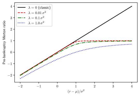
Figure 1. Pre-default Merton ratio $\pi^{\ast}_{\mathrm{pre}}$ vs. $\lambda$

Moreover, for $\mu-r\leq\sigma^{2}$, $\pi^{\ast}_{\mathrm{pre}}(\lambda)$ converges to the classical expression $\frac{\mu-r}{\sigma^{2}}$ as $\lambda\searrow 0$. It is also interesting to observe that our Merton ratio in Equation (45) always suggests to put less money into the stock than the usual Merton ratio would recommend. In particular, it also encourages to short the stock more aggressively, especially for larger $\lambda$, which makes practical sense in view of the chance of default. For $\mu-r<\sigma^{2}$, $\pi^{\ast}_{\mathrm{pre}}(\lambda)\nearrow 1$ as $\lambda\searrow 0$. Unlike classical situation, this means the investor should never invest all of his capital into stock or borrow from the bank to purchase stock. Indeed, since the risk of the stock price to default sporadically over any non-trivial time interval is positive, a Merton ratio $\pi\geq 1$ is not admissible in the sense of Equation (39) as it renders the terminal wealth $Y_{T}$ in Equation (22) zero or negative with a positive probability, therefore, rendering the expected utility equal $-\infty$. This is a major qualitative difference to the classical scenario.

Proposition 1.

The value function is given by

(46) $$V(t,x)=-e^{-\lambda t}\log(x)-\frac{C^{\ast}(\lambda)}{\lambda}\big{(}e^{-\lambda t}-e^{-\lambda T}\big{)}-r\Big{(}T-\frac{1-e^{-\lambda T}}{\lambda}\Big{)}\quad\text{ for }t\geq 0,x>0$$

with $\pi^{\ast}_{\mathrm{pre}}$ from Equation (45) and

$$C^{\ast}(\lambda)=\big{(}\mu\pi^{\ast}_{\mathrm{pre}}+r(1-\pi^{\ast}_{\mathrm{pre}})\big{)}-\frac{1}{2}\sigma^{2}(\pi^{\ast}_{\mathrm{pre}})^{2}+\lambda\log(1-\pi^{\ast}_{\mathrm{pre}}).$$

Proof.

Plugging

$$\partial_{t}V(t,x)=\lambda e^{-\lambda t}\log(x)+\dot{G}(t),\quad\partial_{x}V(t,x)=e^{-\lambda t}(1/x),\quad\partial_{xx}V(t,x)=-e^{-\lambda t}(1/x^{2})$$

into HJB Equation (41), we obtain

$$\lambda e^{-\lambda t}\log(x)+\dot{G}(t)-\big{(}\mu\pi^{\ast}_{\mathrm{pre}}+r(1-\pi^{\ast}_{\mathrm{pre}})\big{)}e^{-\lambda t}+\frac{1}{2}\sigma^{2}(\pi^{\ast}_{\mathrm{pre}})^{2}e^{-\lambda t}-\lambda e^{-\lambda t}\log(1-\pi^{\ast}_{\mathrm{pre}})-\lambda e^{-\lambda t}\log(x)=0$$

or, equivalently,

(47) $$\dot{G}(t)=Ce^{-\lambda t}\text{ for }t\geq 0$$

with

(48) $$C=\big{(}\mu\pi^{\ast}_{\mathrm{pre}}+r(1-\pi^{\ast}_{\mathrm{pre}})\big{)}-\frac{1}{2}\sigma^{2}(\pi^{\ast}_{\mathrm{pre}})^{2}+\lambda\log(1-\pi^{\ast}_{\mathrm{pre}}).$$

Integrating Equation (47), we obtain $G(t)=-\frac{C}{\lambda}e^{-\lambda t}+c$ for some constant $c$. On the strength of Equation (42), we have the terminal condition

$$-\frac{C}{\lambda}e^{-\lambda T}+c=-r\Big{(}T-\frac{1-e^{-\lambda T}}{\lambda}\Big{)},$$

whence $c=\frac{C}{\lambda}e^{-\lambda T}-r\Big{(}T-\frac{1-e^{-\lambda T}}{\lambda}\Big{)}$ and

$$G(t)=\frac{C}{\lambda}\big{(}e^{-\lambda T}-e^{-\lambda t}\big{)}-r\Big{(}T-\frac{1-e^{-\lambda T}}{\lambda}\Big{)}$$

for $t\geq 0$ and $x>0$. ∎

Interestingly, the following observations can be made. For $\mu-r<\sigma^{2}$, using L’Hôpital’s rule, $V(t,x;\lambda)$ can be shown to converge to the classical Merton value function, i.e.,

$$\lim_{\lambda\searrow 0}V(t,x;\lambda)=-\log(x)-\Big{(}r+\frac{(\mu-r)^{2}}{\sigma^{2}}\Big{)}(T-t).$$

In contrast, for $\mu-r>\sigma^{2}$,

$$\lim_{\lambda\searrow 0}V(t,x;\lambda)=-\log(x)-\Big{(}\mu-\frac{1}{2}\sigma^{2}\Big{)}(T-t).$$

since $\lim_{\lambda\searrow 0}\pi^{\ast}_{\mathrm{pre}}(\lambda)=1$ and $\lim_{\lambda\searrow 0}C^{\ast}(\lambda)=\mu-\frac{1}{2}\sigma^{2}$.

Observing

$$V(t,x),\partial_{t}V(t,x),\partial_{xx}V(t,x)\in C^{0}([0,T]\times(0,\infty),\mathbb{R})\text{ with }\partial_{xx}V(t,x)=e^{-\lambda t}x^{-2}>0\text{ and }\pi^{\ast}_{t}\in\mathcal{A}_{tx},$$

the conditions of Verification Theorem [2, Theorem 3] are met, furnishing the following optimality result.

Proposition 2.

Let the wealth process be given by Equation (22).

• The Merton ratio

  $$\pi^{\ast}_{t}=\pi^{\ast}_{\mathrm{pre}}\mathds{1}_{\{t<\tau\}}$$

  with $\pi^{\ast}_{\mathrm{pre}}$ given in Equation (45) minimizes the negative expected utility $J(\pi)$ in Equation (38) over all admissible controls $\pi\in\mathcal{A}_{tx}$ and satisfies

  $$J(\pi^{\ast})=\inf_{\pi\in\mathcal{A}_{tx}}J(\pi)=V(t,x).$$

• The optimal wealth process, $W^{\ast}_{t}$, is given by Equations (20)–(22) with $\pi^{\ast}_{t}$ as above.

5. Example: Bombardier Stock Data Analysis

To illustrate our proposed methodology, we consider the B-rated stock of Bombardier Inc. (BBD-B.TO), a Canadian aerospace and transportation company, quoted by Toronto Stock Exchange. The annualized rating default probability is estimated as $\hat{\lambda}=2.99\%$ [20, Table 23]. For simplicity, we use $\hat{\lambda}=3\%$ in our calculations. Downloading a three years’ worth of daily closing prices from 2912021 to 2912024 from Yahoo! Finance [11], we compute the log-differenced returns

$$X_{i}=\log(S_{t_{i+1}})-\log(S_{t_{i}})\text{ for }i=1,2,\dots,n$$

with $n=751$ furnishing the the annualized drift and volatility estimates (cf. [3, 28])

(49) $$\hat{\mu}=\frac{n_{\mathrm{trade}}}{n}\sum_{i=1}^{n}X_{i},\quad\hat{\sigma}=\sqrt{n_{\mathrm{trade}}}\Big{(}\frac{1}{n-1}\sum_{i=1}X_{i}^{2}-\frac{n}{n-1}\Big{(}\frac{1}{n}\sum_{i=1}^{n}X_{i}\Big{)}^{2}\Big{)}^{1/2}$$

where $n_{\mathrm{trade}}=252$ stands for the number of trading days. See columns 1 and 2 in Table 1.

$\hat{\mu}$	$\hat{\sigma}$	$\hat{\lambda}$	$\hat{\pi}_{\mathrm{classic}}^{\ast}$	$\hat{\pi}_{\mathrm{pre}}^{\ast}$	$\hat{\pi}_{\mathrm{post}}^{\ast}$
$40\%$	$60\%$	$3\%$	$101.12\%$	$74.21\%$	$0\%$

Table 1. Estimated model parameters $\hat{\mu}$, $\hat{\sigma}$, $\hat{\lambda}$ (annualized) and resulting optimal allocations $\hat{\pi}_{\mathrm{classic}}^{\ast}$ (both pre- and post-default) according to Merton and $\hat{\pi}_{\mathrm{pre}}^{\ast}$ and $\hat{\pi}_{\mathrm{post}}^{\ast}$ derived in this paper.

Using Equations , the classical Merton’s ratio $\hat{\pi}_{\mathrm{classic}}^{\ast}$ recommends to invest $101.12\%$ of capital in stock while only $74.32\%$ of capital is allocated in stock pre-default under our new ratio $\hat{\pi}_{\mathrm{pre}}^{\ast}$. In addition to offering a much less conservative investment strategy, classical Merton ratio is not even admissible (cf. Equation (39)) in the presence of a sporadic bankruptcy as it renders the expected terminal utility equal negative infinity. Therefore, the difference between our framework and the classical framework of Merton is not merely quantitative, but qualitative.

6. Summary and Conclusions

In this work, we presented an explicit solution to the optimal wealth allocation problem between a stock and a cash bond assuming the stock bankruptcy is an exogenous event with a constant intensity $\lambda$. To the best of our knowledge, neither this type of problems, nor the solution we developed for the $\log$-utility have previously appeared in the literature. The stochastic integral derivation for this type of processes appears to be new as well. Our solution has an interesting feature that one should never allocates all money in a stock that can go bankrupt to hedge against an entire loss of one’s money. This seems to correlate with the investor behavior in real market. The framework we developed is not limited to bankruptcy events only. In fact, stochastic control problems with regime or security changes can be solve using a similar method. These examples include convertible bonds (i.e., bonds with a conversion feature), bonds with embedded options assuming the probability of embedded options are governed by an exogenous probability, mortgage bonds, etc. Our framework can also be applied in the context of switching between economic regimes caused by exogenous events in the market. We intend to investigate these and other scenarios in subsequent work.

Supplementary Materials

The following materials are available at https://github.com/mpokojovy/MertonAbsorbing:

1. Python code to produce Figure 1.

2. R code implementing the results of Section 5.

Appendix A Auxiliary Results

Lemma 3.

Let $g(t,x,\pi,p,A)=f(t,x,\pi)\cdot p+\frac{1}{2}\sigma^{2}(t,x,\pi)\cdot A-L(t,x,\pi)$ with

$$f(t,x,\pi)=\big{(}\mu\pi+r(1-\pi)\big{)}x,\quad\sigma(t,x,\pi)=\sigma\pi x,\quad L(t,x,\pi)=\lambda e^{-\lambda t}\log\big{(}(1-\pi)x\big{)}.$$

Assuming $x>0$ and $A>0$,

$$\mathop{\operatorname{arg\,min}}_{\pi<1}g(t,x,\pi,p,A) =\pi^{\ast}(t,x,p,A),$$

$$\inf_{\pi<1}g(t,x,\pi,p,A) =g\big{(}t,x,\pi^{\ast}(t,x,p,A),p,A\big{)}$$

with

(50) $$\pi^{\ast}(t,x,p,A)=\frac{-(\mu-r)xp+\sigma^{2}x^{2}A-\sqrt{((\mu-r)xp+\sigma^{2}x^{2}A)^{2}+4\lambda e^{-\lambda t}(\sigma^{2}x^{2}A)}}{2(\sigma^{2}x^{2}A)}.$$

Proof.

The function

$$g(t,x,\pi,p,A)=\big{(}\mu\pi+r(1-\pi)\big{)}x\cdot p+\frac{1}{2}\sigma^{2}\pi^{2}x^{2}\cdot A-\lambda e^{-\lambda t}\log\big{(}(1-\pi)x\big{)}$$

is smooth with respect to all of its arguments $t\geq 0$, $x>0$, $\pi<1$, $p\in\mathbb{R}$ and $A>0$. Since $\lim_{\pi\nearrow 0}g(t,x,\pi,p,A)=\infty$, no minimum can be attained in a vicinity of $\pi=1$.

Computing the derivative

$$\partial_{\pi}g(t,x,\pi,p,A)=(\mu-r)xp+\sigma^{2}\pi x^{2}A+\frac{\lambda e^{-\lambda t}}{1-\pi},$$

the Fermat first-order optimality equation $\partial_{\pi}g(t,x,\pi,p,A)=0$ reads as

$$\sigma^{2}\pi x^{2}A+(\mu-r)xp+\frac{\lambda e^{-\lambda t}}{(1-\pi)}=0$$

or, multiplying with $(\pi-1)$,

(51) $$P(\pi;\lambda t)\equiv\big{(}\sigma^{2}x^{2}A\big{)}\pi^{2}+\big{(}(\mu-r)xp-\sigma^{2}x^{2}A\big{)}\pi-\big{(}(\mu-r)xp+\lambda e^{-\lambda t}\big{)}=0.$$

Solving the former quadratic equation, we obtain two roots given by

$$\pi_{1,2} =\frac{-\big{(}(\mu-r)xp-\sigma^{2}x^{2}A\big{)}\pm\sqrt{\big{(}(\mu-r)xp-\sigma^{2}x^{2}A\big{)}^{2}+4\big{(}\sigma^{2}x^{2}A\big{)}\big{(}(\mu-r)xp+\lambda e^{-\lambda t}\big{)}}}{2\big{(}\sigma^{2}x^{2}A\big{)}}$$

$$=\frac{-\big{(}(\mu-r)xp-\sigma^{2}x^{2}A\big{)}\pm\sqrt{\big{(}(\mu-r)xp+\sigma^{2}x^{2}A\big{)}^{2}+\lambda e^{-\lambda t}\big{(}\sigma^{2}x^{2}A\big{)}}}{2\big{(}\sigma^{2}x^{2}A\big{)}}.$$

In view of $A>0$, both roots are real and satisfy $\pi_{1}\leq\pi_{2}$. Moreover, since $P(\pi;\lambda,t)>P(\pi;0,t)$ for $\lambda>0$ and $t\geq 0$, we observe

$$\pi_{1}(\lambda t)<\pi_{1}(0)\quad\text{ and }\quad\pi_{2}(\lambda t)>\pi_{2}(0)\quad\text{ for }\lambda>0\text{ and }t\geq 0.$$

Consider the following two cases.

• Assuming $(\mu-r)xp\leq\sigma^{2}Ax^{2}$, we obtain

  $$\pi_{1}(\lambda t)<\pi_{1}(0)\equiv-\frac{\mu-r}{\sigma^{2}}\Big{(}\frac{p}{Ax}\Big{)}\leq 1\quad\text{ and }\quad\pi_{2}(\lambda t)>\pi_{2}(0)\equiv 1\text{ for }\lambda>0\text{ and }t\geq 0$$

  and, thus, $\partial_{\pi}g(t,x,\pi,p,A)\leq 0$ for $\pi<\pi_{1}(\lambda t)$ and $\partial_{\pi}g(t,x,\pi,p,A)\geq 0$ for $\pi_{1}(\lambda t)<\pi<1$.

• Otherwise, $(\mu-r)xp>\sigma^{2}Ax^{2}$, which implies

  $$\pi_{1}(\lambda t)<\pi_{1}(0)\equiv 1\quad\text{ and }\quad\pi_{2}(\lambda t)\geq\pi_{2}(0)\equiv-\frac{\mu-r}{\sigma^{2}}\Big{(}\frac{p}{Ax}\Big{)}>1\text{ for }\lambda>0\text{ and }t\geq 0$$

  and, thus, again $\partial_{\pi}g(t,x,\pi,p,A)\leq 0$ for $\pi<\pi_{1}(\lambda t)$ and $\partial_{\pi}g(t,x,\pi,p,A)\geq 0$ for $\pi_{1}(\lambda t)<\pi<1$.

Therefore, in either scenario, the global minimum of $g=g(\pi)$ is attained at $\pi=\pi_{1}(\lambda t)$ for $\lambda>0$, $t\geq 0$ and $x>0$ assuming $A>0$. ∎

References

- [1] Y. Aït-Sahalia and T. R. Hurd. Portfolio choice in markets with contagion. Journal of Financial Econometrics, 14, 2016.
- [2] S. Albosaily and S. Pergamenchtchikov. Optimal investment and consumption for multidimensional spread financial markets with logarithmic utility. Stats, 4:1012–1026, 2021.
- [3] A. T. Anum and M. Pokojovy. A hybrid method for density power divergence minimization with application to robust univariate location and scale estimation. Communications in Statistics – Theory and Methods, 2023.
- [4] N. Azevedo, D. Pinheiro, and G.-W. Weber. Dynamic programming for a Markov-switching jump-diffusion. Journal of Computational and Applied Mathematics, 267:1–19, 2014.
- [5] T. R. Bielecki and I. Jang. Portfolio optimization with a defaultable security. Asia Pacific Financial Markets, 13, 2006.
- [6] M. Brennan, E. Schwartz, and R. Lagnado. Strategic asset allocation. Journal of Economic Dynamics and Control, Volume 21, 1997.
- [7] A. Capponi and J. Figueroa Lopez. Dynamic portfolio optimization with a defaultable security and regime switching. Mathematical Finance, 24, 2011.
- [8] A. Capponi and M. Larsson. Default and systemic risk in equilibrium. Mathematical Finance, 25, 2015.
- [9] S. Emmer and C. Kluppelberg. Optimal portfolios when stock prices follow an exponential Levý process. Finance and Stochastics, 8, 2004.
- [10] W. Fei. Optimal control of uncertain stochastic systems with Markovian switching and its application to portfolio decisions. Cybernetics and Systems – An International Journal, 45, 2014.
- [11] Yahoo! Finance. Bombardier Inc. (BBD-B.TO) Historical Prices. https://finance.yahoo.com/quote/BBD-B.TO/history, February 2024.
- [12] W. H. Fleming and R. W. Rishel. Deterministic and Stochastic Optimal Control, volume 25 of Stochastic Modelling and Applied Probability. Springer, New York, NY, 1975.
- [13] W. H. Fleming and H. M. Soner. Controlled Markov Processes and Viscosity Solutions, volume 25. Springer Science & Business Media, New York, NY, 2006.
- [14] J.-P. Fouque, R. Sircar, and T. Zariphopoulou. Portfolio optimization and stochastic volatility asymptotics. Mathematical Finance, 27(3):704–745, 2017.
- [15] T. Goll and J. Kallsen. Optimal portfolios for logarithmic utility. Stochastic Processes and their Applications, 89:31–48, 2000.
- [16] I. Karatzas, J. Lehoczky, S. Sethi, and S. Shreve. Explicit solution of a general consumption/investment problem. Mathematics of Operations Research, 11(2):261–294, 1986.
- [17] A. Klinger. Control with stochastic stopping time. International Journal of Control, 11:541–549, 1970.
- [18] P. E. Kloeden and E. Platen. Numerical Solution of Stochastic Differential Equations, volume 23 of Stochastic Modelling and Applied Probability. Springer, Berlin, Heidelberg, 1992.
- [19] Y. Kopeliovich. Optimal control problems for stochastic processes with absorbing regime. Journal of Stochastic Analysis, 4, 2023.
- [20] N. W. Kraemer, J. Palmer, N. M. Richhariya, S. Iyer, L. Fernandes, A. Meher, and S. Pranshu. Default, Transition, and Recovery: 2021 Annual Global Corporate Default and Rating Transition Study. https://www.spglobal.com/ratings/en/research/articles/220413-default-transition-and-recovery-2021-annual-global-corporate-default-and-rating-transition-study-12336975, April 2022.
- [21] H. Leland. Corporate debt value, bond covenants, and optimal capital structure. Journal of Finance, 49, 1994.
- [22] H. Leland, R. Goldstein, and N. Ju. An EBIT-based model of optimal capital structure. Journal of Business, 74, 2001.
- [23] T. Lukashiv, Y. Litvinchuk, I.V. Malyk, A. Golebiewska, and P.V. Nazarov. Stabilization of stochastic dynamical systems of a random structure with Markov switches and Poisson perturbations. Mathematics, 11, 2023.
- [24] J. Medhi. Stochastic Processes. New Age International Publishers, New Delhi, 2nd edition, 1984.
- [25] R. Merton. Lifetime portfolio selection under uncertainty: the continuous-time case. The Review of Economics and Statistics, 51, 1969.
- [26] R. Merton. An intertemporal capital asset pricing model. Econometrica, 41, 1973.
- [27] E. Platen and R. Rendek. Exact scenario simulation for selected multi-dimensional stochastic processes. Communications on Stochastic Analysis, 3(3):443–465, 2009.
- [28] M. Pokojovy and A. T. Anum. A fast initial response approach to sequential financial surveillance. In H. Han and E. Baker, editors, The Recent Advances in Transdisciplinary Data Science, pages 19–33, Cham, 2022. Springer Nature Switzerland.
- [29] C. S. Pun and H. Y. Wong. Robust investment?reinsurance optimization with multiscale stochastic volatility. Insurance: Mathematics and Economics, 62:245?256, 2015.
- [30] The Economist. Buttonwood (Online Column). How to avoid a common investment mistake. https://www.economist.com/finance-and-economics/2023/09/21/how-to-avoid-a-common-investment-mistake, September 2023.
- [31] J. Wachter. Portfolio and consumption decisions under mean-reverting returns: An exact solution for complete markets. Journal of Financial And Quantitative Analysis, 37, 2002.
- [32] J. Wei, Y. Shen, and Q. Zhao. Portfolio selection with regime-switching and state-dependent preferences. Journal of Computational and Applied Mathematics, 365:112361, 2020.