Cell-level modelling of homeostasis in confined epithelial monolayers

Abstract

Tissue homeostasis, the biological process of maintaining a steady state in tissue via control of cell proliferation, death, and metabolic function, is essential for the development, growth, maintenance, and proper function of living organisms. Disruptions to this process can lead to serious diseases and even death. In this study, we use the vertex model for the cell-level description of tissue mechanics to investigate the impact of the tissue microenvironment and local mechanical properties of cells on homeostasis in confined epithelial tissues. We find a dynamic steady state, where the balance between cell divisions and removals sustains homeostasis. By characterising homeostasis in terms of cell count, tissue area, and the cells’ neighbour count distribution, we identify the factors that govern regulated and ordered tissue growth. This work, therefore, sheds light on the mechanisms underlying tissue homeostasis and highlights the importance of mechanics in the control of biological processes such as tissue development and disease pathology.

I Introduction

Cell proliferation, the process by which cells grow and multiply through division, is essential for various biological functions such as tissue development, growth, and maintenance [1]. For example, during the early stages of embryonic development cells rapidly proliferate, differentiate, and position themselves to lay out the body plan for the development of a new organism [2]. Throughout adult life, maintaining tissue homeostasis involves a balance between cell proliferation and cell death. This is essential for tissue upkeep, repair, and regeneration in response to injury [3, 4, 5]. Disruptions of this balance can lead to serious diseases such as cancer [6], atherosclerosis [7], and rheumatoid arthritis [8]. Therefore, a key question is how tissues maintain the balance between cell division and cell death to ensure homeostasis.

Tissue homeostasis relies on the delicate balance between cell proliferation and cell death, which are regulated not only by biochemical factors but also by mechanical cues [9, 10]. Cells experience forces from their microenvironment, provided by the surrounding tissues and extracellular matrix [11]. These mechanical forces are often converted into intracellular biochemical signals that influence critical biological processes such as cell adhesion, migration, differentiation, and growth [12]. One such regulatory mechanism exemplifying how mechanical cues influence cellular behaviour is contact inhibition, a process that halts cell division in dense environments to prevent tissue overcrowding and maintain integrity [13, 14]. However, in many cancers, control of cell growth is disrupted, leading to a complex, heterogeneous mixture of actively dividing and quiescent cells, along with the necrotic tissue [15, 16]. In addition, the mechanical forces exerted by the microenvironment strongly impact cancerous growth by regulating the stresses imposed on a tumour, highlighting the critical role of mechanics in tumour progression [17]. Despite its central importance, our understanding of the mechanical processes that control tissue homeostasis remains limited.

Furthermore, understanding the mechanical regulation of cell proliferation is important for identifying physical mechanisms that underlie the development of higher organisms. For example, in amniotes such as birds and reptiles, embryos before gastrulation [2] (i.e. the developmental process in which an embryo transforms into a multilayered three-dimensional structure) are a flat disk of epithelial cells consisting of two main tissue types, the epiblast or embryonic tissue in the centre, and the extra-embryonic tissue encircling it [18]. Cell divisions and ingressions (i.e. removal of the cells into the region below the epiblast) occur throughout the epiblast, effectively maintaining its integrity during gastrulation  [18, 19, 20]. The extra-embryonic tissue, on the other hand, provides mechanical tension to the epiblast [21], which is essential for the proper execution of gastrulation. It also serves critical roles in nutrient transport, waste elimination, and providing protective barriers [22].

In this paper, we explore how the tissue microenvironment and cell mechanical properties contribute to establishing and maintaining homeostasis in confined planar epithelia. Various approaches have been proposed to simulate the mechanics of epithelial cells, including particle-based approaches [23, 24, 25], phase-field methods [26, 27, 28, 29], cellular Potts models [30, 31], Voronoi models [32, 33], and, notably, vertex models [34, 35, 36, 37]. Here, we use the vertex model to investigate homeostasis in confined epithelial tissues with two coexisting components, an active proliferating tissue surrounded by a passive non-proliferating tissue.

We demonstrate that mechanical forces suffice to sustain homeostasis, resulting in a dynamic steady state characterised by a balance between the number of cell divisions and ingressions. We find that the homeostatic state is sensitive to the mechanical properties of both the active and passive tissues as well as the strength of the confinement. In particular, the steady-state area of the proliferating part decreases with decreasing stiffness of the proliferating tissue and increasing stiffness of the surrounding non-proliferating tissue. Furthermore, growth can also be regulated by increasing the confinement strength for a given set of mechanical properties of the tissue. These findings highlight the potential for manipulating the characteristics of the tissue microenvironment to regulate its growth and emphasize the significance of mechanics in regulating tissue-scale processes.

This paper is organised as follows: In Sec. II, we provide details of the two-dimensional vertex model for epithelial tissue mechanics, including the implementation of cellular processes within this framework. In Sec. III, we present our findings by characterising homeostasis in terms of the variation in the (i) number of active cells, (ii) area occupied by active cells, (iii) polygonal distribution of the active cell shapes, and (iv) realised shape index (i.e. the ratio of cell perimeter to the square root of its area) of the active tissue. Specifically, Sec. III.1 describes the temporal dynamics as the system progresses towards homeostasis, and Sec. III.2 discusses the sensitivity of the homeostatic state to the target shape indexes of active and passive cells. Then, in Sec. III.3, we present the analysis of the effect of confinement on homeostasis.

II Model

II.1 Two-dimensional vertex model for epithelial tissue mechanics

Epithelial cells are tightly packed to form a confluent monolayer (e.g. epiblast of amniote embryos, the lining of blood vessels, kidney tubules, intestine, etc.) or a multilayer (e.g. skin, excretory ducts of sweat glands, etc.) sheet [38]. The tissue cohesion is achieved by an adhesion belt formed of clusters of E-cadherin molecules concentrated in the adherens junctions [39], giving epithelial tissues elastic properties. While the shapes of cells in an epithelial monolayer resemble prisms, the molecules primarily responsible for the generation and transmission of mechanical forces are located close to the apical side (i.e. the top surface) of the cells. Therefore, a common approach is to focus on the apical side alone and approximate the tissue as a two-dimensional polygonal tiling. Cells are thus represented as polygons that share junctions, and three or more junctions meet at a vertex. This description is known as the two-dimensional vertex model [34, 35, 37].

The mechanical energy of the model epithelium is determined by cell shapes, and it is given as

$$E=\sum_{c\,\in\,\text{cells}}\left[\frac{K_{A}}{2}(A_{c}-A_{c,0})^{2}+\frac{K_{P}}{2}(P_{c}-P_{c,0})^{2}\right],$$ (1)

where the sum is over all the cells in the tissue. The first term is the penalty associated with changes in the cell’s area, $A_{c}$, from a reference value $A_{c,0}$, and it accounts for the volume conservation and preferred height of actual cells. The second term penalises deviations in the cell’s perimeter, $P_{c}$, from a reference value, $P_{c,0}$, and models the mechanical properties of the adhesion belt. The associated elastic moduli are $K_{A}$ and $K_{P}$, respectively. In general, the reference areas and perimeters, as well as the two elastic moduli, can be cell-type dependent. In Eqn. (1), the dependence of the moduli is, however, omitted to declutter the notation.

Equation (1) can be transformed into a dimensionless form using a characteristic length scale $l^{*}$, the choice of which will be discussed below. One then divides both sides of Eqn. (1) with $K_{P}l{{}^{*}}^{2}$ to obtain

$$e=\frac{1}{2}\sum_{c\,\in\,\text{cells}}\Big{[}{k}_{A}(a_{c}-a_{c,0})^{2}+(p_{c}-p_{c,0})^{2}\Big{]},$$ (2)

where ${k}_{A}=\left(K_{A}l{{}^{*}}^{2}\right)/K_{P}$, $a_{c}=A_{c}/l{{}^{*}}^{2}$, $a_{c,0}=A_{c,0}/l{{}^{*}}^{2}$, $p_{c}=P_{c}/l^{*}$, and $p_{c,0}=P_{c,0}/l^{*}$. For convenience, we did not absorb the prefactor $1/2$ into the definition of dimensionless constants. Therefore, the product $K_{P}l{{}^{*}}^{2}$ sets the unit of energy.

If all cells have the same target areas, $A_{0}$, and perimeters, $P_{0}$, a typical choice of length scale is $l^{*}=\sqrt{A_{0}}$. In this case, Eqn. (2) can be further simplified as,

$$e=\frac{1}{2}\sum_{c\,\in\,\text{cells}}\Big{[}{k}_{A}(a_{c}-1)^{2}+(p_{c}-p_{0})^{2}\Big{]}.$$ (3)

The ratio $p_{0}=P_{0}/\sqrt{A_{0}}$ is called the target shape index, and it determines the tissue’s mechanical behaviour, distinguishing fluid–like and solid–like responses. Once $p_{0}$ exceeds a critical value, the shear modulus of the tissue decreases to zero, and the tissue fluidises. This is accompanied by the disappearance of the energy barrier for cell neighbour exchanges [40]. For a tissue made entirely of hexagonal cells, the shear modulus falls to zero at the critical value $p_{0}=6/\sqrt{3\sqrt{3}/2}\approx 3.722$, i.e. the perimeter to the square root of the area ratio of a regular hexagon. However, the energy barriers for neighbour exchanges remains finite until $p_{0}\approx 3.81$, the corresponding ratio of a regular pentagon [41]. For random tilings, the solid-fluid transition has been reported to be in the range $p_{0}\approx 3.81-3.92$ [42, 43, 44, 45]. Lastly, if $A_{c,0}$ and $P_{c,0}$ are cell-dependent, a typical choice for the length scale is $l^{*}=\sqrt{\bar{A}_{0}}$, where $\bar{A}_{0}$ is the average of $A_{c,0}$ over all cells.

Cells in epithelial tissues are dynamic, but their motion is slow ($\sim 10\,$µm/h). Therefore, the motion is overdamped and can be approximated as a force balance between dissipative and mechanical forces. Under the assumption that cells are supported by a substrate that provides most of the dissipation via dry friction, the equation of motion for the vertex $i$ at the position $\mathbf{r}_{i}$ is

$$\zeta\dot{\mathbf{r}}_{i}=\mathbf{F}_{i}.$$ (4)

The overdot represents the time derivative, $\zeta$ is the friction coefficient, and $\mathbf{F}_{i}$ is the force on the vertex. If only passive mechanical forces are present, $\mathbf{F}_{i}=-\nabla_{\mathbf{r}_{i}}E$, where $\nabla_{\mathbf{r}_{i}}$ is the gradient with respect to the position vector $\mathbf{r}_{i}$ of vertex $i$, and mechanical energy $E$ is defined in Eqn. (1). In the presence of activity, $\mathbf{F}_{i}$ can be extended to include additional force contributions [46, 47]. Following the same steps as above, the equation of motion can be non-dimensionalised, resulting in the unit of time $t^{*}=\zeta/K_{P}$. Finally, we have omitted the noise term that would normally accompany the dissipative term in the equation of motion [48] since the effects of the microscopic noise on the long-time behaviour of cells in epithelial tissue are usually negligible.

To maintain proper function, epithelial cells rearrange via neighbour exchanges, grow, divide, and die. Therefore, the vertex dynamics needs to be augmented to include cellular processes such as intercalations (i.e. cell neighbour exchanges), ingression/extrusion (i.e. removal of individual cells from the tissue), cell division, and cell growth. Modelling these processes requires updates of the connectivity of the polygonal tiling via topological changes such as T1 (intercalation) and T2 (ingression/extrusion) transitions [36].

II.2 An active inclusion in a passive tissue patch

We use the two-dimensional vertex model to study a square patch of size $L_{\text{a}}\times L_{\text{a}}$ of a proliferating active epithelial tissue embedded in a passive epithelium confined to a square box of size $L\times L$. The passive tissue is clamped to the edges of the box, as illustrated in Fig. 2a. Passive cells can move and rearrange, but cannot grow, divide, or be extruded. Active cells, however, can grow, divide, and be extruded.

We initialise the simulation with a disordered tiling generated by placing $N$ points at random in a square box. The disks act as the initial seeds for a Voronoi tessellation. Upon building the Voronoi tesselation, the seed points are moved to the centroids of Voronoi tiles, and a new Voronoi tiling is constructed. The procedure is repeated iteratively until the maximal relative difference between positions of seed points in two consecutive iterations is below $5\cdot 10^{-5}$. This results in a centroidal Voronoi tesselation, which has the property that the tiling is random, but all cells are of similar size and shape [49]. We sample the dimensionless target areas of cells in the active tissue ($a_{c,0}^{\text{a}}$) from a normal distribution with a mean of $1$ and a standard deviation of $\sigma$. The corresponding target perimeters of the active cells are determined by $p_{c,0}^{\text{a}}=p_{0}^{\text{a}}\sqrt{a_{c,0}^{\text{a}}}$, where $p_{0}^{\text{a}}$ is the target shape index of active cells. For the passive cells, the target areas and perimeters are set to constant values $1$ and $p_{0}^{\text{p}}$, respectively. Furthermore, the vertices of the outermost layers are fixed in position and constrained to lie along a straight line, reflecting a clamped boundary condition [50]. Straight boundaries are created during the initial configuration setup by padding the simulation box and mirroring seed points within a preset cutoff distance from the boundaries.

Before starting the full simulation, each random initial configuration is evolved for $10^{4}$ simulation steps (i.e. time $t=50$) without cell growth, divisions, and ingressions. This allows the cells to adapt to their assigned target areas and perimeters. Unless stated otherwise, simulations were performed from a single initial configuration.

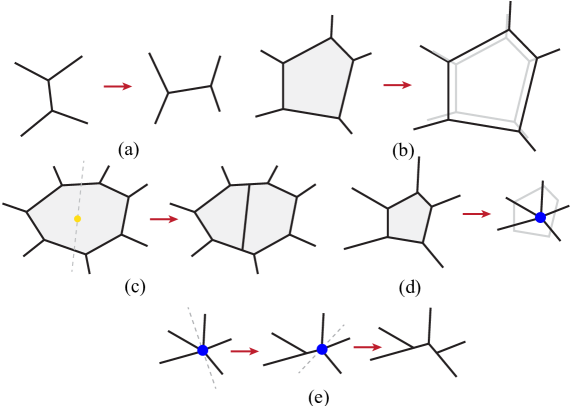
Figure 1: Five morphological changes of the model tissue. (a) Intercalation (i.e. cell neighbour exchange) is implemented via a T1 transition where a junction shorter than a threshold length $\ell_{T1}$ is rotated $90^{\circ}$ counterclockwise and vertex connectivity is updated. (b) Cell growth is implemented by scaling the preferred area $a_{c,0}$. (c) Cells are divided perpendicular to their long axis along a line that passes through the centroid with a probability that is a function of the cell size [Eqn. (6)]. (d) Cells are removed with a probability that is a function of the cell size [Eqn. (7)], by collapsing cell edges into a single vertex. (e) Vertices with four or more neighbours are resolved by spitting them at random while ensuring that mesh connectivity is not violated.

Cell intercalations are implemented via a T1 transition (Fig. 1a) based on a minimum junction length [51]. If the junction length drops below a specified threshold, $\ell_{\text{T1}}$, it is rotated by $90^{\circ}$ counterclockwise and extended to the length $\ell_{\text{T1}}^{\text{n}}=1.02\ell_{\text{T1}}$. Then the connectivity is updated to account for the exchange of cell neighbours. Moreover, T1 transitions rarely result in either a passive cell entering the proliferating region (i.e. it is surrounded only by active cells), or an active cell entering the passive region (i.e. it is surrounded only by passive cells). In these cases, the cell type is changed from passive to active, or vice-versa.

For simplicity, we assume that the cell growth (Fig. 1b) is described by a linear model, where the target area of active cells, $a^{\text{a}}_{c,0}(t)$, evolves as

$$\dot{a}^{\text{a}}_{c,0}=g,$$ (5)

where $g$ is a constant growth rate. The target shape index of active cells is kept constant at $p_{0}^{\text{a}}$ by adjusting the target perimeter to $p^{\text{a}}_{c,0}(t)=p_{0}^{\text{a}}\sqrt{a^{\text{a}}_{c,0}(t)}$. The target area and perimeter of all passive cells are assumed to be identical and time-independent, giving the target shape index $p_{0}^{\text{p}}$. Note that we use $l^{*}=\sqrt{A^{\text{p}}_{0}}$ (i.e. square root of the target passive cell area) in the non-dimensionalisation procedure to avoid the problem of time-dependent simulation units.

Cells in the active region can divide, and the division mechanism is stochastic. The division probability, $\mathbb{P}_{\text{d}}(c)$, of a cell $c$ increases with the cell area $a_{c}$ as

$$\mathbb{P}_{\text{d}}(c)=\frac{1}{1+e^{-\alpha(a_{c}-a_{\text{d}})}},$$ (6)

where $a_{\text{d}}$ represents the area at which the probability of cell division is $1/2$ and $\alpha$ regulates the sensitivity of division probability to changes in the cell area. The division probability is calculated for each cell at each simulation time step, and cell division occurs if a uniformly distributed random number drawn from the interval $[0,1]$ is smaller than the calculated probability $\mathbb{P}_{\text{d}}(c)$. The division process follows Hertwig’s rule [52], i.e. a cell is divided into two daughter cells by choosing a direction perpendicular to its long axis that passes through its centroid (Fig. 1c). The long axis is determined by diagonalising the gyration tensor [53]. The reference areas of two daughter cells are separately drawn from the normal distribution with unit mean and standard deviation $\sigma$ and reference perimeters are calculated as $p_{\text{daughter},0}^{\text{a}}=p_{0}^{\text{a}}\sqrt{a_{\text{daughter,0}}^{\text{a}}}$.

Similarly, for cell ingression, we define the probability $\mathbb{P}_{\text{i}}(c)$ which increases with a decrease in cell area $a_{c}$ as,

$$\mathbb{P}_{\text{i}}(c)=\frac{e^{-\beta(a_{c}-a_{\text{i}})}}{1+e^{-\beta(a_{c}-a_{\text{i}})}},$$ (7)

where $a_{\text{i}}$ represents the area at which the probability of cell ingression is $1/2$ and $\beta$ regulates the sensitivity of ingression probability to changes in the cell area. Ingression of a cell typically leads to the formation of a vertex with more than three neighbours (Fig. 1d). Such vertices are resolved by picking a random “cut” direction that does not violate the tissue connectivity and inserting a new edge of length $\ell_{\text{T1}}^{\text{n}}$. The procedure is repeated until all high-coordination vertices are resolved (Fig. 1e).

These five morphological transformations of the model tissue are shown schematically in Fig. 1. Finally, the equations of motion [Eqn. (4)] are solved using the first-order Euler method with a time step $\delta t$. The parameters and the values used are listed in Table 1.

Table 1: Values of the dimensionless parameters

Parameter	Description	Value
${k}_{A}$	Area elastic modulus	7.5
$\sigma$	Standard deviation of active cells target area	$2.0\cdot 10^{-5}$
$g$	Growth rate	$4.0\cdot 10^{-4}$
$a_{\text{d}}$	Area at which $\mathbb{P}_{\text{d}}(c)=0.5$	$1.6$
$a_{\text{i}}$	Area at which $\mathbb{P}_{\text{i}}(c)=0.5$	$0.3$
$\ell_{\text{T1}}$	T1 transition threshold	$3.17\cdot 10^{-3}$
$\delta t$	Simulation time step	$5\cdot 10^{-3}$
$\alpha$	Division probability sensitivity to cell area	$20.0$
$\beta$	Ingression probability sensitivity to cell area	$15.0$
$p_{0}^{\text{a}}$	Target shape index of active cells	$3.600-3.825$
$p_{0}^{\text{p}}$	Target shape index of passive cells	$3.600-3.825$

III Results and Discussion

III.1 Temporal dynamics of the tissue

We first study the time evolution of the tissue towards homeostasis, as depicted in Fig. 2. Cells in the central proliferating region grow, divide, ingress, and rearrange. Consequently, the region expands and exerts compressive stress on the passive cells, leading to their deformation and intermittent rearrangements. Constrained by the fixed boundary of the simulation box, the passive cells get compressed. Eventually, the system reaches a steady state (i.e. homeostasis), characterised by continuously replenishing cells in the proliferating region.

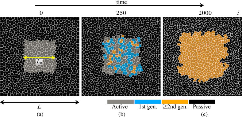
Figure 2: The snapshots of the evolution of the model tissue: (a) initial configuration with active inclusion containing $169$ cells (light grey) surrounded by passive tissue with $831$ cells (black); (b) intermediate configuration showing cells born in the active region after the first division ($1^{\text{st}}$ generation - blue) and subsequent divisions ($\geq 2^{\text{nd}}$ generation - orange); and (c) a steady-state configuration with all initial active cells replaced by new generation cells. These snapshots correspond to $L_{\text{a}}=12.65$, $L=31.62$, $p_{0}^{\text{a}}=3.60$, and $p_{0}^{\text{p}}=3.80$.

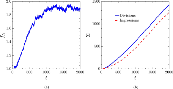
Figure 3: The time dependence of (a) the fractional change in the number of active cells ($f_{N}$) defined in Eqn. (8) and (b) the cumulative sum () of cell divisions (blue) and ingressions (red). $L_{\text{a}}=12.65$, $L=31.62$, $p_{0}^{\text{a}}=3.60$, and $p_{0}^{\text{p}}=3.80$.

Figure 3 shows the time evolution of the fractional change in the number of active cells,

$$f_{N}(t)=\frac{N_{\text{a}}(t)}{N_{\text{a}}(t=0)},$$ (8)

where $N_{\text{a}}(t)$ is the number of active cells at time $t$, and the cumulative sums, $(t)$, of cell divisions and ingressions as the system reaches homeostasis. The active cell population gradually increases until $t\approx 1500$, and reaches a dynamic steady state where $f_{N}$ saturates but continues to fluctuate around a mean value (the plateau in Fig. 3a). The state is characterised by a dynamical balance between divisions and ingressions (Fig. 3b), i.e. the cumulative sums of cell divisions and ingressions continuously grow but retain, on average, a constant difference.

III.2 Effects of target shape index of active and passive cells

We characterise the homeostatic state in terms of the steady-state mean values of the fractional change in the number ($\bar{f}_{N}$) and the area ($\bar{f}_{A}$) of active cells defined, respectively, as

$$\bar{f}_{N}=\frac{1}{N_{T}}\sum_{i=1}^{N_{T}}f_{N}(t_{i})\quad\text{and}\quad\bar{f}_{A}=\frac{1}{N_{T}}\sum_{i=1}^{N_{T}}f_{A}(t_{i}).$$ (9)

Here, the averaging is done for $N_{T}=2\cdot 10^{4}$ simulation steps corresponding to the time interval $\Delta t=500$, with data recorded every five steps. The averaging is started after the time $t_{1}=1500$, which is longer than it typically takes for the system to reach the dynamic steady state (Appendix A). $f_{N}$ is defined in Eqn. (8), and, analogously, $f_{A}=A_{\text{a}}(t)/A_{\text{a}}(t=0)$ denotes the fractional change in the area occupied by the active cells, $A_{\text{a}}$.

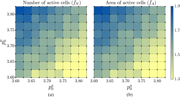
Figure 4: The mean fractional change of (a) the number of active cells, $\bar{f}_{N}$, and (b) the area occupied by the active cells, $\bar{f}_{A}$, [Eqns. (9)] as a function of the target shape index of active ($p_{0}^{\text{a}}$) and passive ($p_{0}^{\text{p}}$) cells. The colour bar applies to both panels. $L_{\text{a}}=12.65$ and $L=31.62$. Simulations are performed at grid points indicated by black circles, and the colour within each square represents the average of the values at the four corners of that square. The standard deviation of the time series used to compute the mean values is within the range of $0.01-0.05$.

Figure 4a shows that the final cell count of active cells measured in terms of $\bar{f}_{N}$ is sensitive to the target shape indexes of both passive, $p_{0}^{\text{p}}$, and active, $p_{0}^{\text{a}}$, cells. Specifically, for a given value $p_{0}^{\text{a}}$, the mean fractional change of the number of active cells, $\bar{f}_{N}$, increases as $p_{0}^{\text{p}}$ is increased from $3.600$ to $3.825$. Conversely, $\bar{f}_{N}$ decreases with increasing $p_{0}^{\text{a}}$. This dependency of $\bar{f}_{N}$ on $p_{0}$ can be understood as follows. Increasing $p_{0}$ makes the tissue softer and reduces the energy costs associated with neighbour exchanges. Therefore, an increase in $p_{0}^{\text{p}}$ softens the passive tissue, thus enabling easier deformation of passive cells. Conversely, an increase in $p_{0}^{\text{a}}$ softens the active cells, rendering them less effective in compressing the passive cells.

Furthermore, the sensitivity of the mean steady area fraction of active cells, $\bar{f}_{A}$, to variation of $p_{0}^{\text{a}}$ and $p_{0}^{\text{p}}$, shown in Fig. 4b, mirrors the trends observed in the cell count (Fig. 4a). Similar to the cell count, the area of the active tissue increases with an increase in the target shape index $p_{0}^{\text{p}}$ of passive cells and decreases with an increase in the target shape index $p_{0}^{\text{a}}$ of active cells. Therefore, a stiffer proliferating tissue enclosed by softer passive tissue results in a homeostatic state with maximum cell count and area.

III.2.1 Disorder in the active tissue

Here, we quantify the disorder in the active tissue in terms of the distribution of the cell neighbour count and the realised shape index of active cells.

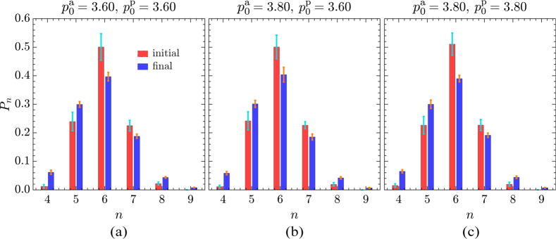
Figure 5: Fraction of active cells, $P_{n}$, as a function of the number of cell neighbours, $n$, averaged over five different initial configurations for different target shape index combinations: (a) $p_{0}^{\text{a}}=3.60$, $p_{0}^{\text{p}}=3.60$, (b) $p_{0}^{\text{a}}=3.80$, $p_{0}^{\text{p}}=3.60$, and (c) $p_{0}^{\text{a}}=3.80$, $p_{0}^{\text{p}}=3.80$. The initial and final distributions, averaged across all realisations, are denoted by red and blue bars, respectively, with error bars indicating the corresponding standard deviations of the mean values. $L_{\text{a}}=12.65$ and $L=31.62$, and the mean is calculated over $N_{T}=2\cdot 10^{4}$ simulation time steps (i.e. time interval $T=500$ with the data recorded every five simulation steps) in the steady state.

Figure 5 shows the mean distribution of cell neighbour counts averaged over five different initial configurations (generated as outlined in Sec. II.2) for different combinations of target shape indexes of active and passive cells. The transition from the initial (red bars) to the steady-state distribution (blue bars) illustrates how cells reorganise. In agreement with the previous studies [35, 54, 55], regardless of the values of $p_{0}^{\text{a}}$ and $p_{0}^{\text{p}}$, the distribution exhibits a pattern where hexagons dominate the tiling, followed by pentagons, heptagons and quadrilaterals. Furthermore, comparing the initial configuration with the final dynamic configuration reveals a decrease in the fraction of hexagons and an increase in the fraction of pentagons, irrespective of the target shape indexes. This suggests that the continuous divisions and ingressions contribute to tissue disorder by increasing the fraction of pentagons and decreasing the fraction of hexagons. Lastly, the final distribution of cell neighbour counts remains qualitatively insensitive to the cell neighbour count distribution of the initial configurations that are in the class of well-centred Voronoi tilings (see Sec. II.2).

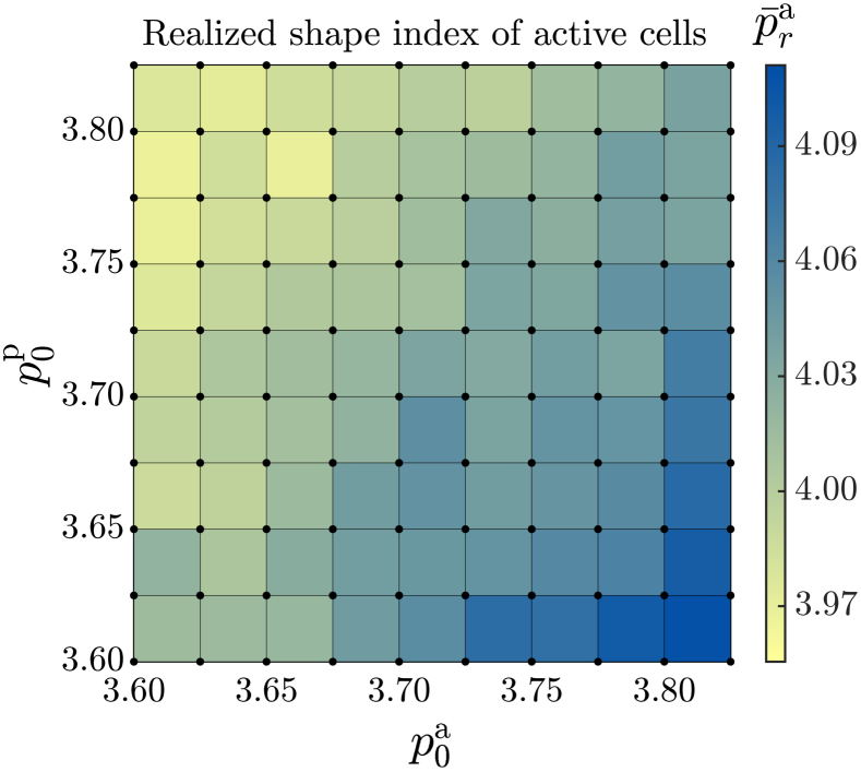
Figure 6: The dependence of realised steady-state shape index of active cells, $\bar{p}_{\text{r}}^{\text{a}}$, on the target shape indices of active, $p_{0}^{\text{a}}$, and passive, $p_{0}^{\text{p}}$, cells. $L_{\text{a}}=12.65$ and $L=31.62$. Simulations are performed at grid points indicated by black circles, and the colour within each square represents the average of the values at the four corners of each square. The standard deviation of the time series used to compute the mean values is within the range of $0.006-0.018$.

To gain further insight into the impact of target shape indexes on tissue morphology, we explore the dependence of the mean realised steady-state shape index of the active tissue, $\bar{p}_{\text{r}}^{\text{a}}$, on the input target shape indexes $p_{0}^{\text{a}}$ and $p_{0}^{\text{p}}$, as shown in Fig. 6. $\bar{p}_{\text{r}}^{\text{a}}$ is calculated as

$$\bar{p}_{\text{r}}^{\text{a}}=\frac{1}{N_{T}}\sum_{i=1}^{N_{T}}\left(\frac{1}{N_{\text{a}}(t_{i})}\sum_{c}p_{\text{r},c}^{\text{a}}(t_{i})\right),$$ (10)

where $p_{\text{r},c}^{\text{a}}(t_{i})=p_{c}(t_{i})/\sqrt{a_{c}(t_{i})}$ represents the realised shape index of the cell $c$ at simulation step $t_{i}$, with $p_{c}(t_{i})$ and $a_{c}(t_{i})$, respectively, being the perimeter and area of the cell $c$, and $t_{1}$ and $N_{T}$ are the same as in Eqns. (9). The mean realised shape index, $\bar{p}_{\text{r}}^{\text{a}}$, increases with increasing $p_{0}^{\text{a}}$ and decreasing $p_{0}^{\text{p}}$. Since large values of the shape index correspond to more fluid-like tissues with less regular cell shapes, this indicates that the tissue becomes more disordered as the active tissue gets softer and the passive tissue stiffens.

In summary, the optimal configuration for efficient tissue proliferation, characterised by maximum cell count and reduced disorder, involves stiffer proliferating tissue enclosed by softer passive tissue.

III.3 Effects of confinement - varying the width of the passive tissue

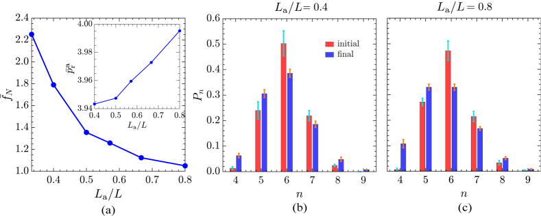
Figure 7: (a) Dependence of the fractional change in the number of active cells, $\bar{f}_{N}$ on the width of the passive region, quantified by the ratio $L_{\text{a}}/L$; Inset: the realised shape index of active cells, $\bar{p}_{\text{r}}^{\text{a}}$, as a function of $L_{\text{a}}/L$, for $p_{0}^{\text{a}}=3.60$ and $p_{0}^{\text{p}}=3.80$. (b) and (c) Corresponding probability distributions of cell neighbour counts of the active tissue averaged over five different initial configurations for weaker and stronger confinements, respectively. The error bars represent one standard deviation of the five mean values.

Finally, we investigate the effect of confinement, quantified by the ratio $L_{\text{a}}/L$, on the homeostatic state of the active tissue. By keeping the initial size of the active tissue constant at $L_{\text{a}}=12.65$, we systematically vary $L$ to modify the thickness of the passive tissue and, thus, the strength of the confinement. Reducing $L_{\text{a}}/L$ corresponds to weakening the confinement due to the presence of a thick layer of passive tissue between the active tissue and the fixed boundary, which shields the active region from the effects of the fixed boundaries. Conversely, the $L_{\text{a}}/L\to 1$ case corresponds to strong confinement, as there is only a thin layer of passive tissue, and the active patch can easily sense the boundary of the simulation box.

Figure 7 shows how changes in $L_{\text{a}}/L$ impact the fractional change in the number of active cells and the cell neighbour count distribution. We choose $p_{0}^{\text{a}}=3.60$ and $p_{0}^{\text{p}}=3.80$ as it results in efficient tissue proliferation (Fig. 4) with less disorder (Fig. 6). As shown in Fig. 7a, the cell count monotonically decreases with a decrease in the thickness of the passive tissue (i.e. as confinement strengthens). This is because the clamped boundary emulates a fully rigid tissue, and strengthening the confinement enhances the impact of the fixed boundary on the active tissue. Consequently, making confinement stronger yields effects similar to reducing $p_{0}^{\text{p}}$ (Fig. 4).

Furthermore, Figs. 7b,c show the mean distribution of the number of cell neighbours of the active tissue averaged over five different initial configurations for weaker ($L_{\text{a}}/L=0.4$) and stronger ($L_{\text{a}}/L=0.8$) confinements, respectively. In weaker confinements, hexagons dominate the tiling, followed by pentagons, and then heptagons, whereas in stronger confinements, there is no significant difference between the fraction of hexagons and pentagons (blue bars). However, comparing the initial equilibrium configuration with the final dynamic configuration reveals a decrease in the fraction of hexagons and an increase in the fraction of pentagons irrespective of confinement. Moreover, the fraction of quadrilaterals is higher in strong confinements compared to weak confinements. Thus, strong confinements favour cells with $\leq 5$ neighbours in the active region, whereas weak confinement favours hexagonal cells. Therefore, the disorder in the active tissue increases as confinement becomes stronger. This is evident in the inset of Fig. 7a, which depicts that the realised shape index of active cells ($\bar{p}_{\text{r}}^{\text{a}}$) increases as the confinement becomes stronger, akin to the effect observed when $p_{0}^{\text{p}}$ is decreased. Finally, in the steady state, the mean distribution of the number of cell neighbours remains qualitatively insensitive to the cell neighbour distribution in the initial configurations that are in the class of well-centred Voronoi tilings of the plane (see Sec. II.2).

IV Summary and Conclusions

In this paper, we used the two-dimensional vertex model for cell-level modelling of tissue mechanics to investigate homeostasis in confined epithelial tissues consisting of a central region populated with actively proliferating cells and a surrounding region occupied by non-proliferating passive cells. We showed that the system can reach homeostasis which is a dynamic steady state maintained by a balance between cell divisions and ingressions. We characterised the homeostatic state of the tissue in terms of the fractional change in the number of active cells, the area occupied by the active cells, and the distribution of cell shapes. Notably, these parameters demonstrate sensitivity to the mechanical properties of both the active and passive cells, as quantified by their respective target shape indices. Moreover, we observed that the strength of confinement significantly influences the homeostatic state. Our findings illustrate a simple mechanism that regulates the growth of a confined tissue and establishes homeostasis.

The fractional change in the number of active cells and the area occupied by them increases with an increase in the target shape index of the passive cells and decreases with an increase in the target shape index of the active cells. Thus, an optimal layout for controlling the growth of a confined tissue involves a softer active tissue confined by a stiffer passive tissue characterised by a higher target shape index of active cells and a lower target shape index of passive cells. However, this configuration results in greater disorder within the proliferating tissue, as indicated by a significantly higher realized shape index. Additionally, the strength of confinement (i.e. the thickness of the passive region) significantly alters the homeostatic state. As confinement gets stronger, i.e. as the thickness of the passive region decreases, the cell count decreases, while the realised shape index increases, mirroring the effect of decreasing the shape index of the passive cells. However, strong confinement also affects the cells’ neighbour count distribution, favouring cells with $\leq 5$ neighbours in the active region.

This study emphasizes the central role of cells’ mechanical properties, alongside the tissue microenvironment, in regulating homeostasis, providing valuable insights into tissue maintenance. By demonstrating the sensitivity of the homeostatic state to variations in mechanical factors, such as confinement strength and tissue stiffness, our findings highlight the intricate interplay between mechanical cues and cellular behaviour. This emphasizes that a complete description of biological processes at tissue and organ scales necessitates biochemical and mechanical approaches, applied at the same footing.

Appendix A Active cell count - sensitivity to initial configuration

Here, we discuss the sensitivity of the change in active cell count to the initial configuration. Different initial configurations are generated according to the procedure outlined in Section II.2.

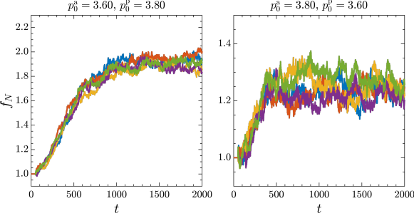
Figure 8: The time dependence of the fractional change in the number of active cells is shown for five different initial configurations for (a) $p_{0}^{\text{a}}=3.60$, $p_{0}^{\text{p}}=3.80$, and (b) $p_{0}^{\text{a}}=3.80$, $p_{0}^{\text{p}}=3.60$. Each curve in both panels corresponds to a different initial configuration. $L_{\text{a}}=12.65$ and $L=31.62$.

Figure 8 shows the time evolution of the fractional change in the number of active cells for five different realisations. Specifically, it highlights the shape index combinations resulting in high ($p_{0}^{\text{a}}=3.60$, $p_{0}^{\text{p}}=3.80$) and low ($p_{0}^{\text{a}}=3.80$, $p_{0}^{\text{p}}=3.60$) changes in the active cell count. The final cell count of active cells is nearly insensitive to the initial configuration. Additionally, as discussed in Sec. III.1, $f_{N}$ increases and saturates to a mean value.