Integrated path stability selection

Abstract.

Stability selection is a widely used method for improving the performance of feature selection algorithms. However, stability selection has been found to be highly conservative, resulting in low sensitivity. Further, the theoretical bound on the expected number of false positives, E(FP), is relatively loose, making it difficult to know how many false positives to expect in practice. In this paper, we introduce a novel method for stability selection based on integrating the stability paths rather than maximizing over them. This yields a tighter bound on E(FP), resulting in a feature selection criterion that has higher sensitivity in practice and is better calibrated in terms of matching the target E(FP). Our proposed method requires the same amount of computation as the original stability selection algorithm, and only requires the user to specify one input parameter, a target value for E(FP). We provide theoretical bounds on performance, and demonstrate the method on simulations and real data from cancer gene expression studies.

1.  Introduction

Stability selection is a popular method for improving feature selection algorithms (Meinshausen and Bühlmann, 2010). It is attractive due to its generality, simplicity, and theoretical control on the expected number of false positives, E(FP), sometimes denoted EV and called the per-family error rate elsewhere in the literature. Despite these favorable qualities, existing theory for stability selection—which heavily informs its implementation—provides relatively weak bounds on E(FP), resulting in a diminished number of true positives (Ahmed et al., 2011; Alexander and Lange, 2011; Hofner et al., 2015; Li et al., 2013; Wang et al., 2020). Furthermore, stability selection requires users to specify two of three parameters: the target E(FP), a selection threshold, and the expected number of selected features. Many works have shown that stability selection is overly sensitive to these choices, making it difficult to tune for good performance (Haury et al., 2012; Li et al., 2013; Wang et al., 2020; Werner, 2023; Zhou et al., 2013).

The limitations of stability selection are illustrated in Figure 1. Here, we consider the canonical example of a linear model $Y_{i}=\beta^{\mathtt{T}}X_{i}+\epsilon_{i}$ for $i\in\{1,\dots,n\}$, where $X_{i}\in\mathbb{R}^{p}$, $n=200$, and $p=1000$ (Wang et al., 2020). Simulated features and noise are generated as $X_{ij}\sim\mathcal{N}(0,1)$ independently, and $\epsilon_{i}\sim\mathcal{N}(0,\sigma^{2})$ independently given $X_{1},\ldots,X_{n}$, where $\sigma^{2}=\sum_{i=1}^{n}(\beta^{\mathtt{T}}X_{i})^{2}/(2n)$ so that the signal-to-noise ratio (SNR) is $2$. The coefficient vector $\beta$ has $s=20$ nonzero entries at coordinates randomly selected from $\{1,\ldots,p\}$, all with $0.5\leq|\beta_{j}|\leq 1$. The results in Figure 1 are obtained by simulating $100$ random data sets as above, and running stability selection using lasso (Tibshirani, 1996) as the baseline feature selection algorithm. A selected feature is called a true positive if its corresponding $\beta$ entry is nonzero, and is a false positive otherwise.

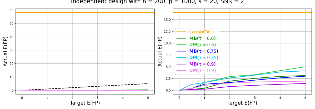
Figure 1. Tradeoff between FP and TP. Stability selection is overly conservative, yielding an extremely small FP at the expense of a small TP, where FP = number of false positives and TP = number of true positives. Meanwhile, lasso has a high TP, but it comes at the expense of a high FP. (Left) Average FP versus target E(FP) for the stability selection methods of Meinshausen and Bühlmann (2010) (MB) and Shah and Samworth (2013) (UM) at several thresholds $\tau$, as well as lasso with cross-validation, which does not depend on the horizontal axis. The black dotted line is the target E(FP). (Right) Average TP versus target E(FP) for the same methods.

The horizontal axis in Figure 1 is the target value of the expected number of false positives (the target E(FP)), which is specified by the user for all variants of stability selection shown. The vertical axes show the actual numbers of false positives (FP) and true positives (TP), averaged over the 100 data sets. Stability selection yields only 2 to 5 true positives on average (selecting $10$-$25\%$ of the $20$ features with $\beta_{j}\neq 0$), and usually has zero false positives (selecting none of the $980$ features with $\beta_{j}=0$). On the other hand, lasso with regularization parameter chosen by cross-validation (LassoCV) produces around $16$ true positives, but $58$ false positives. This is a known trade-off: Stability selection is typically too conservative for feature selection, while lasso with cross-validation is typically not conservative enough (Alexander and Lange, 2011; Leng et al., 2006; Zou, 2006).

In this article, we introduce integrated path stability selection (IPSS), which provides better control over the number of false positives, yielding more true positives compared to stability selection. Specifically, we show that IPSS satisfies a bound on $\mathrm{E(FP)}$ that is orders of magnitude stronger than the corresponding bounds for stability selection. Consequently, for a given target value of E(FP), IPSS typically has many more true positives than stability selection. This is a key advantage since, in practice, the actual number of false positives is unknown, so the stronger bound of IPSS enables one to increase the true positive rate while maintaining guaranteed control over $\mathrm{E(FP)}$. Another advantage of IPSS is that it requires just one user-specified parameter, the target $\mathrm{E(FP)}$. This makes IPSS easier to use than stability selection which, in addition to the target $\mathrm{E(FP)}$, requires one to specify either the selection threshold or the expected number of selected features, and it can be difficult to know how to set these. Finally, IPSS is simple to implement and requires no more computation than stability selection. An IPSS software package is available for download.

The rest of the article is organized as follows. In Section 2, we introduce our proposed methodology. Section 3 provides a brief review of previous work. In Section 4, we present our theoretical results. Section 5 contains an extensive simulation study, and in Section 6, we apply IPSS to identify genes related to prostate and colon cancer. We conclude in Section 7 with a brief discussion.

2.  Integrated path stability selection

In this section, we define the setup of the problem (Section 2.1), describe the stability selection algorithm (Section 2.2), and introduce IPSS (Section 2.3).

2.1.  Setup.

Suppose $S\subseteq\{1,\ldots,p\}$ is an unknown subset to be estimated from independent and identically distributed data $Z_{1},\ldots,Z_{n}$. Let $\hat{S}_{\lambda}(Z_{1:n})\subseteq\{1,\ldots,p\}$ be an estimator of $S$, where $Z_{1:n}=(Z_{1},\ldots,Z_{n})$ and $\lambda>0$ is a parameter. For example, in the regression setting, $Z_{i}=(X_{i},Y_{i})$ where $X_{i}\in\mathbb{R}^{p}$ is a vector of features and $Y_{i}\in\mathbb{R}$ is a response variable for each $i\in\{1,\ldots,n\}$. As illustrated in Section 1, a canonical estimator in this setting is the lasso algorithm (Tibshirani, 1996), in which case $\hat{S}_{\lambda}(Z_{1:n})=\{j:\hat{\beta}_{j}\neq 0\}$ where

$$\hat{\beta} =\operatorname*{arg\,min}_{\beta\in\mathbb{R}^{p}}\,\frac{1}{2}\sum_{i=1}^{n}(Y_{i}-\beta^{\mathtt{T}}X_{i})^{2}+\lambda\sum_{j=1}^{p}|\beta_{j}|.$$

In an unsupervised learning setting, we might have $Z_{i}=X_{i}\in\mathbb{R}^{p}$, without a response variable, such as in the case of graphical lasso (Friedman et al., 2008). See Meinshausen and Bühlmann (2010, Section 2) for details on applying stability selection to graphical lasso as well as other examples of feature selection algorithms amenable to stability selection. We allow $\hat{S}_{\lambda}$ to be a random function, such as in a stochastic optimization algorithm.

We will frequently need to compute the estimator using a subset of the data, say, $Z_{A}=(Z_{i}:i\in A)$ for a given $A\subseteq\{1,\ldots,n\}$. In this case, we write $\hat{S}_{\lambda}(Z_{A})$ to denote the estimator computed using only the data in $Z_{A}$. A key quantity is the probability that feature $j$ is selected when computing the estimator on half of the data. We denote this selection probability by

$$\pi_{j}(\lambda) =\mathbb{P}\big{(}j\in\hat{S}_{\lambda}(Z_{1:\lfloor n/2\rfloor})\big{)}.$$ (2.1)

Stability selection and IPSS employ resampling-based estimators of $\pi_{j}(\lambda)$ computed using Algorithm 1. To be precise, $\pi_{j}(\lambda)$ and the estimated selection probabilities $\hat{\pi}_{j}(\lambda)$ defined in Algorithm 1 depend on $n$, but $n$ is suppressed from notation since we always treat it as an arbitrary fixed value.

Algorithm 1 (Estimated selection probabilities)

1:Data $Z_{1},\ldots,Z_{n}$, selection algorithm $\hat{S}$, parameter grid $\Lambda$, and number of iterations $B$.

2:for $b=1,\ldots,B$ do

3:     Randomly select $A_{2b-1},A_{2b}\subseteq\{1,\ldots,n\}$ with $A_{2b-1}\cap A_{2b}=\varnothing$ and $\lvert A_{2b-1}\rvert=\lvert A_{2b}\rvert=\lfloor n/2\rfloor$.

4:     for $\lambda\in\Lambda$ do

5:         Evaluate $\hat{S}_{\lambda}(Z_{A_{2b-1}})$ and $\hat{S}_{\lambda}(Z_{A_{2b}})$.

6:     end for

7:end for

8:Estimated selection probabilities $\hat{\pi}_{j}(\lambda)=\frac{1}{2B}\sum_{b=1}^{2B}\operatorname{\mathds{1}}\!\big{(}j\in\hat{S}_{\lambda}(Z_{A_{b}})\big{)}$ for $j\in\{1,\ldots,p\}$.

Here, $\operatorname{\mathds{1}}(\cdot)$ denotes the indicator function: $\operatorname{\mathds{1}}(E)=1$ if $E$ is true and $\operatorname{\mathds{1}}(E)=0$ otherwise. Note that $\hat{S}_{\lambda}$ is evaluated on both disjoint subsets, $A_{2b-1}$ and $A_{2b}$, at each iteration of Algorithm 1. This technique of using complementary pairs of subsets was introduced by Shah and Samworth (2013). By contrast, in the original stability selection algorithm of Meinshausen and Bühlmann (2010), $\hat{S}_{\lambda}$ is applied to only one subset of size $\lfloor n/2\rfloor$ at each iteration. Interestingly, this slight modification simplifies the assumptions needed for the theory; see Shah and Samworth (2013).

2.2.  Stability selection.

The set of features selected by stability selection is

$$\hat{S}_{\mathrm{MB}} =\Big{\{}j:\max_{\lambda\in\Lambda_{\mathrm{MB}}}\hat{\pi}_{j}(\lambda)\geq\tau\Big{\}}$$ (2.2)

where $\Lambda_{\mathrm{MB}}\subseteq(0,\infty)$ is a certain interval defined below and $\tau\in(0,1)$ is a user-specified threshold. The subscript MB distinguishes the version of stability selection introduced by Meinshausen and Bühlmann (2010) from the unimodal version (UM) of Shah and Samworth (2013). In practice, the maximum in Equation 2.2 is approximated by computing $\hat{\pi}_{j}(\lambda)$ on a finite grid within $\Lambda_{\mathrm{MB}}$.

An issue with the stability selection procedure is that as $\lambda\to 0$, many or even all features satisfy $\hat{\pi}_{j}(\lambda)\geq\tau$. Consequently, to avoid selecting nearly all features, it is necessary to restrict $\Lambda_{\mathrm{MB}}$ to an interval $[\lambda_{\mathrm{MB}},\lambda_{\mathrm{max}}]$. The upper endpoint $\lambda_{\mathrm{max}}$ is inconsequential provided it is large enough that all features have small selection probability, which is readily obtained in practice. However, choosing $\lambda_{\mathrm{MB}}$ is considerably more subtle, and there is no consensus on how to choose it (Li and Zhang, 2017; Zhou et al., 2013). A standard approach to choosing $\lambda_{\mathrm{MB}}$ proceeds as follows.

First, two of the following three quantities are specified: (i) the target $\mathrm{E(FP)}$, which we denote by $\mathrm{E(FP)}_{*}$, (ii) the threshold, $\tau$, and (iii) the expected number of features selected, $q_{*}$. The third quantity is then determined by setting $\mathrm{E(FP)}_{*}=q_{*}^{2}/(2\tau-1)p$ and solving. This equation comes from the following bound proven by Meinshausen and Bühlmann (2010): letting $q=\mathrm{E}\big{\lvert}\textstyle{\bigcup}_{\lambda\in\Lambda_{\mathrm{MB}}}\hat{S}_{\lambda}(Z_{1:\lfloor n/2\rfloor})\big{\rvert}$,

$$\mathrm{E(FP)} \leq\frac{q^{2}}{(2\tau-1)p}.$$ (2.3)

Once $q_{*}$ is determined, $\lambda_{\mathrm{MB}}=\sup\big{\{}\lambda\in(0,\lambda_{\mathrm{max}}):\mathrm{E}\big{\lvert}\textstyle{\bigcup}_{\lambda^{\prime}\in[\lambda,\lambda_{\mathrm{max}}]}\hat{S}_{\lambda^{\prime}}(Z_{1:\lfloor n/2\rfloor})\big{\rvert}\geq q_{*}\big{\}}$ is empirically estimated (Meinshausen and Bühlmann, 2010), and $\Lambda_{\mathrm{MB}}=[\lambda_{\mathrm{MB}},\lambda_{\mathrm{max}}]$ is used in Equation 2.2. The UM version is the same except that the third quantity is solved for by setting $\mathrm{E(FP)}_{*}=C(\tau,B)\,q_{*}^{2}/p$ for a certain constant $C(\tau,B)$, which comes from Equation 4.9. The resulting $q_{*}$—which is possibly different from the $q_{*}$ in the MB procedure—is then used to define $\lambda_{\mathrm{UM}}$ via the same equation as $\lambda_{\mathrm{MB}}$. Then, $\Lambda_{\mathrm{UM}}=[\lambda_{\mathrm{UM}},\lambda_{\mathrm{max}}]$ is used instead of $\Lambda_{\mathrm{MB}}$ in Equation 2.2 to define $\hat{S}_{\mathrm{UM}}$.

The above construction of $\lambda_{\mathrm{MB}}$ and $\lambda_{\mathrm{UM}}$ elucidates some of the limitations of stability selection and motivates our formulation of IPSS. First, both Equations 2.3 and 4.9 are inequalities, so while the recommended procedure does typically keep the actual $\mathrm{E(FP)}$ smaller than $\mathrm{E(FP)}_{*}$, it may be much smaller, as shown in Figures 1 and 3. This leads to the overly conservative nature of stability selection, in part because $q_{*}$ could have been chosen to be much larger while still satisfying $\mathrm{E(FP)}\leq\mathrm{E(FP)}_{*}$. Second, the right sides of Equations 2.3 and 4.9 go to $\infty$ as $\tau\to 0.5$. It is therefore recommended by Meinshausen and Bühlmann (2010) to take $\tau\in[0.6,0.9]$; however, stability selection is sensitive to $\tau$ even when restricted to this interval (Li et al., 2013; Wang et al., 2020). Nevertheless, $\tau$ must be specified in most cases because it is often unclear what $q_{*}$ should be a priori. Third, the bounds in Equations 2.3 and 4.9 are relatively weak (Figure 3). As a result, $\lambda_{\mathrm{MB}}$ and $\lambda_{\mathrm{UM}}$ tend to be too large, cutting off stability paths before the information they carry can be brought to bear. This contributes to the overly conservative nature of stability selection illustrated in Section 1: Weak bounds lead to large values of $\lambda_{\mathrm{MB}}$ and $\lambda_{\mathrm{UM}}$, which prevent true features from being selected because their selection paths have not yet distinguished themselves from the noise. This phenomenon can be seen in Figure 2 where only one feature exceeds the $\tau=0.75$ threshold before reaching the stability selection endpoint, $\lambda_{\mathrm{MB}}$, and two features exceed $\tau=0.75$ before $\lambda_{\mathrm{UM}}$. In this example, $\mathrm{E(FP)}_{*}=1$, so one false positive is permitted on average, but there were zero false positives in both cases. By contrast, seven features are selected by IPSS, six of which are true positives and one of which is a false positive, agreeing with the target $\mathrm{E(FP)}$.

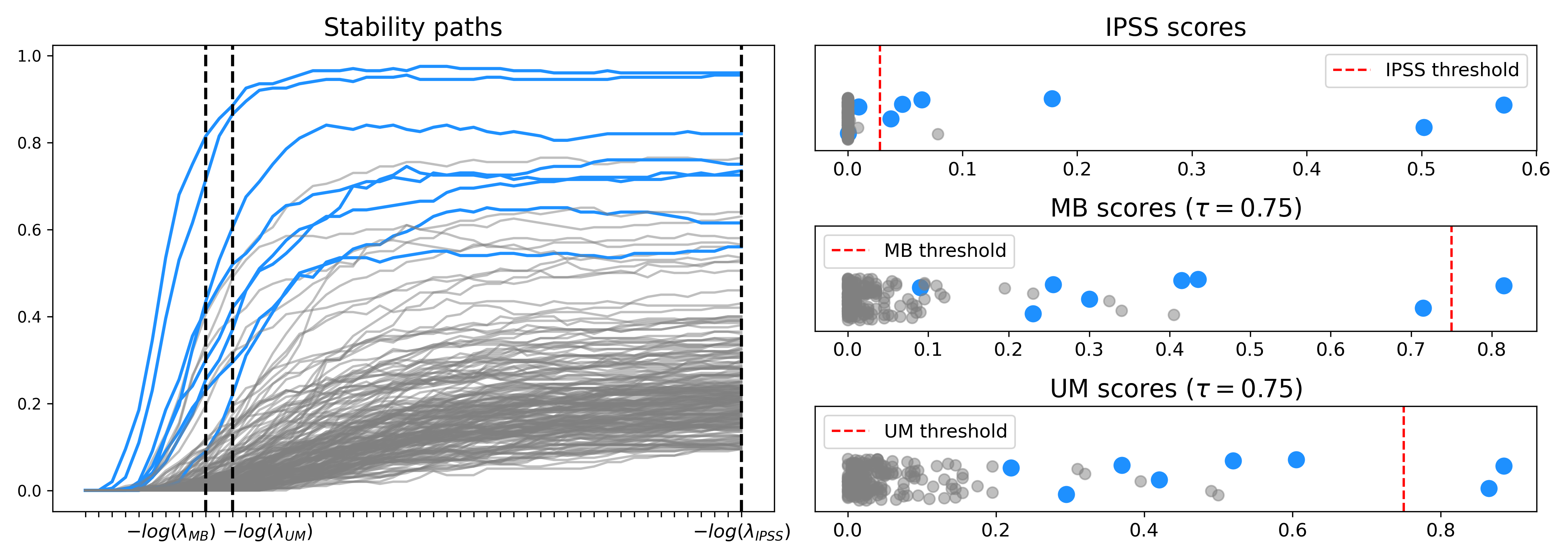
Figure 2. (Left) Estimated stability paths $\hat{\pi}_{j}(\lambda)$ for linear regression with independent design as in Section 1. Here $n=100$, $p=200$, $\mathrm{SNR}=1$, and there are $s=8$ true features, shown in blue. The horizontal axis is a grid of $50$ regularization parameters, evenly spaced on a log scale from $-\log(\lambda_{\mathrm{max}})$ to $-\log(\lambda_{\mathrm{IPSS}})$. Note that $\lambda_{\mathrm{UM}}$ is only slightly smaller than $\lambda_{\mathrm{MB}}$, while $\lambda_{\mathrm{IPSS}}$ is significantly smaller than both $\lambda_{\mathrm{MB}}$ and $\lambda_{\mathrm{UM}}$. (Right) Feature scores for IPSS (top), MB stability selection (middle), and UM stability selection (bottom), along with their respective thresholds (vertical red lines) separating selected and unselected features. Scores are one-dimensional and correspond to the horizontal axes; the vertical displacement is random jitter, solely for better visualization. For stability selection, the scores are the maxima of the selection probabilities over the interval between $\lambda_{\mathrm{max}}$ and $\lambda_{\mathrm{MB}}$ or $\lambda_{\mathrm{UM}}$, which in this case is determined by setting $\tau=0.75$ and $\mathrm{E(FP)}_{*}=1$. IPSS scores are given by Equation 2.4 with $f=h_{3}$, defined in Equation 2.5. MB and UM have $\mathrm{TP}=1$ and $\mathrm{TP}=2$, respectively, and $\mathrm{FP}=0$ in both cases. IPSS has $\mathrm{TP}=6$ and $\mathrm{FP}=1$.

2.3.  Integrated path stability selection.

The set of features selected by IPSS is

$$\hat{S}_{\mathrm{IPSS},f} =\Big{\{}j:{\int}_{\Lambda}f(\hat{\pi}_{j}(\lambda))\mu(d\lambda)\geq\tau\Big{\}}$$ (2.4)

where $\Lambda$ is a subinterval of $(0,\infty)$, $f:[0,1]\to\mathbb{R}$, $\mu$ is a probability measure on $\Lambda$, and $\tau$ is a threshold. We provide our recommended choices of $\Lambda$, $f$, $\mu$, and $\tau$ below, but our theory holds more generally and other choices may perform even better. In practice, IPSS is performed by computing $\hat{\pi}_{j}(\lambda)$ on a grid within $\Lambda$ using Algorithm 1, then applying the criterion in Equation 2.4 with a numerical approximation to the integral; see details below.

The two basic differences between IPSS and stability selection are: (i) IPSS integrates rather than maximizes, and (ii) IPSS typically considers a much wider range of $\lambda$ values. Consequently, IPSS incorporates more information from the selection paths, compared to stability selection. This translates into stronger theoretical results (Section 4) and empirical performance (Sections 5 and 6).

The function $f$. The role of $f$ in Equation 2.4 is to transform the selection probabilities $\hat{\pi}_{j}$ to improve performance. While any $f:[0,1]\to\mathbb{R}$ could be used, we focus on functions of the form

$$h_{m}(x) =(2x-1)^{m}\operatorname{\mathds{1}}(x\geq 0.5)$$ (2.5)

where $m\in\mathbb{N}$. (The $h$ stands for “half”, since $h_{m}$ is positive on half of the unit interval.) We recommend $h_{3}$ for lasso ($L^{1}$-regularized linear regression) and $h_{2}$ for $L^{1}$-regularized logistic regression; these choices are used in all of the examples. However, $h_{2}$ and $h_{3}$ worked nearly equally well on both linear and logistic regression, suggesting that they are good choices in general.

The measure $\mu$. The probability measure $\mu$ on $\Lambda$ in Equation 2.4 weights the regularization parameters $\lambda$. As with $f$, any choice of $\mu$ could be used in general, but we recommend using $\mu_{1}(d\lambda)=z_{1}^{-1}\lambda^{-1}d\lambda$ where $z_{1}=\int_{\Lambda}\lambda^{-1}d\lambda$ is a normalizing constant. The probability measure $\mu_{1}$ corresponds to averaging on a logarithmic scale; see Section S1.2 for details on integrating with respect to $\mu_{1}$.

The interval $\Lambda$. Like stability selection, IPSS requires the specification of $\Lambda$, which we choose to be an interval $\Lambda_{\mathrm{IPSS}}=[\lambda_{\mathrm{IPSS}},\lambda_{\mathrm{max}}]$ constructed as follows. The upper endpoint $\lambda_{\mathrm{max}}$ is the same as in stability selection and equally inconsequential. The lower endpoint $\lambda_{\mathrm{IPSS}}$ is based on a bound of the form $\mathrm{E(FP)}\leq\mathcal{I}(\lambda,\lambda_{\mathrm{max}})/\tau$ where $\mathcal{I}(\lambda,\lambda_{\mathrm{max}})$ is an integral over $[\lambda,\lambda_{\mathrm{max}}]$ that depends on the choice of $f$; see Sections 4 and S3 for the precise formulas. We define

$$\lambda_{\mathrm{IPSS}} =\inf\big{\{}\lambda\in(0,\lambda_{\mathrm{max}}):\mathcal{I}(\lambda,\lambda_{\mathrm{max}})\leq C\big{\}},$$ (2.6)

where $C>0$ is an integral cutoff value that we always set to $C=0.05$, though any $C\in[0.02,0.15]$ yields similar results. Further details about the construction of $\Lambda_{\mathrm{IPSS}}$, including the specific choice of $\lambda_{\mathrm{max}}$ and the evaluation of Equation 2.6, are in Section S1.1.

The threshold $\tau$. Once $\Lambda_{\mathrm{IPSS}}=[\lambda_{\mathrm{IPSS}},\lambda_{\mathrm{max}}]$ and $\mathrm{E(FP)}_{*}$ (the target E(FP)) are specified, we set

$$\tau=\frac{\mathcal{I}(\lambda_{\mathrm{IPSS}},\lambda_{\mathrm{max}})}{\mathrm{E(FP)}_{*}}.$$

Note that the exact infimum in Equation 2.6 satisfies $\mathcal{I}(\lambda_{\mathrm{IPSS}},\lambda_{\mathrm{max}})=C$, but in practice there is a small approximation error, so $\tau$ is not exactly $C/\mathrm{E(FP)}_{*}$. Intuitively, the role of $C$ is to reparametrize the width of the interval over which stability paths are integrated, so that $C$ is invariant to the problem at hand. If the interval is too small, then the selection paths will be cut off prematurely, making it difficult to distinguish true features from noise. On the other hand, if the interval is too large, then $\tau$ will be too large, and the IPSS criterion becomes overly conservative.

Computation. Algorithm 2 is a step-by-step description of IPSS. Our general parameter recommendations are $B=50$, $f=h_{3}$ (lasso) or $f=h_{2}$ (logistic regression), $\mu=\mu_{1}$, $C=0.05$, and $r\in\{25,50\}$. Results are similar whether $r=25$ or $50$; using $r=25$ speeds up computation when running IPSS on a large number of data sets as we do in our simulation studies, while $r=50$ yields more refined stability paths. These are the parameter settings used for all examples in this work.

Algorithm 2 (Integrated path stability selection)

1:Data $Z_{1},\ldots,Z_{n}$, selection algorithm $\hat{S}$, number of iterations $B$, function $f$, measure $\mu$, target $\mathrm{E(FP)}_{*}$, integral cutoff value $C$, and number of grid points $r$.

2:Compute $\lambda_{\mathrm{IPSS}}$ and $\lambda_{\mathrm{max}}$ as described above and in Section S1.1.

3:Partition $\Lambda_{\mathrm{IPSS}}=[\lambda_{\mathrm{IPSS}},\lambda_{\mathrm{max}}]$ into $r$ grid points, typically on a log scale.

4: Compute $\mathcal{I}(\lambda_{\mathrm{IPSS}},\lambda_{\mathrm{max}})$ using the relevant upper bound on $\mathrm{E(FP)}$ and S1.1.

5:Set $\tau=\mathcal{I}(\lambda_{\mathrm{IPSS}},\lambda_{\mathrm{max}})/\mathrm{E(FP)}_{*}$.

6:Estimate selection probabilites via Algorithm 1 with $Z_{1},\dots,Z_{n}$, $\hat{S}$, $\Lambda_{\mathrm{IPSS}}$, and $B$.

7:Approximate IPSS scores $\hat{s}_{j}=\int_{\Lambda_{\mathrm{IPSS}}}f(\hat{\pi}_{j}(\lambda))\mu(d\lambda)$ using S1.1.

8:Selected features $\hat{S}_{\mathrm{IPSS},f}=\{j:\hat{s}_{j}\geq\tau\}$.

The upper bounds referred to in step 4 are in Theorem 4.2 for $h_{m}$. The integrals required for IPSS can be accurately and efficiently approximated by a simple Riemann sum for a wide range of functions $f$ and measures $\mu$; see S1.1 for details. Indeed, we find no discernible difference in computation time between IPSS and stability selection. This is unsurprising in light of the fact that stability selection and IPSS both estimate the selection probabilities via Algorithm 1, which is much more expensive than evaluation of either Equation 2.2 or Equation 2.4. For more on the computational requirements of Algorithm 1, see Meinshausen and Bühlmann (2010, Section 2.6).

3.  Previous work

Stability selection was introduced by Meinshausen and Bühlmann (2010) and refined by Shah and Samworth (2013). These remain the preeminent works on stability selection and are the most commonly implemented versions to date. Zhou et al. (2013) provide the only other work we are aware of that aims to improve upon the selection criterion in Equation 2.2 and the $\mathrm{E(FP)}$ bound. They propose top-$k$ stability selection, which averages over the $k$ largest selection probabilities for each feature. The special case of $k=1$ is stability selection. While Zhou et al. (2013) provide theory for top-$k$ stability selection, their improvement upon the $\mathrm{E(FP)}$ upper bound of Meinshausen and Bühlmann (2010) is considerably weaker than the improved bound provided by IPSS; compare Zhou et al. (2013, Theorem 3.1) to our Theorem 4.1. Moreover, introducing $k$ increases the number of settings to choose, and it is shown that results are sensitive to $k$ (Zhou et al., 2013).

It is far more common for stability selection to be modified on an ad hoc basis to mitigate its sensitivity to parameters and overly conservative results. An example is the popular TIGRESS method of Haury et al. (2012), which uses stability selection to infer gene regulatory networks. To reduce sensitivity to the stability selection parameters, they use a selection criterion that averages over selection probabilities. It turns out that this is the special case of IPSS with $f(x)=x$ (the function $w_{1}$ in Section S3) and $\mu=\mu_{1}$. Another example is in the work of Maddu et al. (2022), where stability selection is used to learn differential equations. There the authors use a selection criterion based only on selection probabilities at the smallest regularization parameter.

Finally, another common approach is to use stability selection in conjunction with other methods. Examples include stability selection with boosting (Hofner et al., 2015) and grouping features prior to applying stability selection, which has been done in genome-wide association studies (Alexander and Lange, 2011). IPSS is equally amenable to such approaches and can replace stability selection in such methods at no additional computational cost and with fewer required parameters.

4.  Theory

In this section, we present our theoretical results (Section 4.2) and compare these results to those of Meinshausen and Bühlmann (2010) and Shah and Samworth (2013) (Section 4.3). Our main result, Theorem 4.1, establishes a bound on $\mathrm{E(FP)}$ when using IPSS. Theorem 4.2 gives simplified formulas for this bound that we use in practice. The proofs of all results in this section are in Section S2. Additional results for other choices of $f$ and their proofs are in Section S3.

4.1.  Preliminaries.

It is assumed that the random variables $Z_{1},\dots,Z_{n}$, the random subsets $A_{1},\dots,A_{2B}$, and any randomness in the feature selection algorithm $\hat{S}$ are all defined on a common probability space $(\Omega,\mathcal{F},\mathbb{P})$. Furthermore, $\mathrm{E}$ always denotes expectation with respect to $\mathbb{P}$. Let $\Lambda$ be a Borel measurable subset of $(0,\infty)$ equipped with the Borel sigma-algebra, let $\mu$ be a probability measure on $\Lambda$, and assume $\hat{S}_{\lambda}(Z_{A})$ is measurable as a function on $\Lambda\times\Omega$ for all $A\subseteq\{1,\dots,n\}$.

4.2.  Main results.

The following condition is used in Theorem 4.1. Recall that $S$ is the unknown subset of true features, and $S^{c}=\{1,\ldots,p\}\setminus S$ denotes the complement of $S$. Let $q(\lambda)=\mathrm{E}\lvert\hat{S}_{\lambda}(Z_{1:\lfloor n/2\rfloor})\rvert$ denote the expected number of variables selected by $\hat{S}_{\lambda}$ on half the data.

Condition 1.

We say Condition 1 holds for $m$ if for all $\lambda\in\Lambda$,

$$\max_{j\in S^{c}}\,\mathbb{P}\bigg{(}j\in\bigcap_{b=1}^{m}\big{(}\hat{S}_{\lambda}(Z_{A_{2b-1}})\cap\hat{S}_{\lambda}(Z_{A_{2b}})\big{)}\bigg{)} \leq(q(\lambda)/p)^{2m}.$$ (4.1)

Equation 4.1 says the probability that any non-true feature $j$ is selected by both $\hat{S}_{\lambda}(Z_{A_{2b-1}})$ and $\hat{S}_{\lambda}(Z_{A_{2b}})$ in $m$ distinct trials is no greater than the $2m$th power of the expected proportion of features selected by $\hat{S}_{\lambda}$ using half the data.

Theorem 4.1.

Let $\tau\in(0,1]$ and $m\in\mathbb{N}$. Define $\hat{S}_{\mathrm{IPSS},h_{m}}$ as in Equations 2.4 and 2.5. If Condition 1 holds for all $m^{\prime}\in\{1,\ldots,m\}$, then

$$\mathrm{E(FP)} =\mathrm{E}\lvert\hat{S}_{\mathrm{IPSS},h_{m}}\cap S^{c}\rvert\leq\frac{p}{\tau B^{m}}\sum_{k_{1}+\cdots+k_{B}=m}\frac{m!}{k_{1}!k_{2}!\cdots k_{B}!}\int_{\Lambda}(q(\lambda)/p)^{2\sum_{b}\operatorname{\mathds{1}}(k_{b}\neq 0)}\mu(d\lambda)$$ (4.2)

where $B$ is the number of subsampling steps in Algorithm 1 and the sum is over all nonnegative integers $k_{1},\ldots,k_{B}$ such that $k_{1}+\cdots+k_{B}=m$.

Equation 4.2 bounds the expected number of false positives when using IPSS with $h_{m}$. The following theorem shows that the bound can be simplified considerably for certain choices of $m$.

Theorem 4.2.

Let $\tau\in(0,1]$. If Condition 1 holds for $m=1$, then IPSS with $h_{1}$ satisfies

$$\mathrm{E(FP)} \leq\frac{1}{\tau}\int_{\Lambda}\frac{q(\lambda)^{2}}{p}\mu(d\lambda);$$ (4.3)

if Condition 1 holds for $m\in\{1,2\}$, then IPSS with $h_{2}$ satisfies

$$\mathrm{E(FP)} \leq\frac{1}{\tau}\int_{\Lambda}\bigg{(}\frac{q(\lambda)^{2}}{Bp}+\frac{(B-1)q(\lambda)^{4}}{Bp^{3}}\bigg{)}\mu(d\lambda);$$ (4.4)

and if Condition 1 holds for $m\in\{1,2,3\}$, then IPSS with $h_{3}$ satisfies

$$\mathrm{E(FP)} \leq\frac{1}{\tau}\int_{\Lambda}\bigg{(}\frac{q(\lambda)^{2}}{B^{2}p}+\frac{3(B-1)q(\lambda)^{4}}{B^{2}p^{3}}+\frac{(B-1)(B-2)q(\lambda)^{6}}{B^{2}p^{5}}\bigg{)}\mu(d\lambda).$$ (4.5)

Taking the limit as $B\to\infty$, the cases of $h_{2}$ and $h_{3}$ in Equations 4.4 and 4.5 become

$$\limsup_{B\to\infty}\mathrm{E(FP)} \leq\frac{1}{\tau p^{3}}\int_{\Lambda}q(\lambda)^{4}\mu(d\lambda)\quad\text{and}\quad\limsup_{B\to\infty}\mathrm{E(FP)}\leq\frac{1}{\tau p^{5}}\int_{\Lambda}q(\lambda)^{6}\mu(d\lambda),$$ (4.6)

respectively. Although we do not use these asymptotic bounds, the pattern from $h_{1}$ (Equation 4.3) to $h_{2}$ to $h_{3}$ (Equation 4.6) provides insight into relationships between $\mathrm{E(FP)}$, $p$, and $h_{m}$.

Condition 1 holds for $m=1$ whenever $\max_{j\in S^{c}}\pi_{j}(\lambda)\leq q(\lambda)/p$ for all $\lambda\in\Lambda$ since $Z_{1},\ldots,Z_{n}$ are i.i.d. and independent of $A_{1},\ldots,A_{2B}$, and thus for any non-true feature $j$,

$$\mathbb{P}\big{(}j\in\hat{S}_{\lambda}(Z_{A_{2b-1}})\cap\hat{S}_{\lambda}(Z_{A_{2b}})\big{)} =\mathrm{E}\Big{(}\mathrm{E}\big{(}\operatorname{\mathds{1}}(j\in\hat{S}_{\lambda}(Z_{A_{2b-1}}))\operatorname{\mathds{1}}(j\in\hat{S}_{\lambda}(Z_{A_{2b}}))\;\big{|}\;A_{2b},A_{2b-1}\big{)}\Big{)}$$

$$=\mathrm{E}\big{(}\pi_{j}(\lambda)\pi_{j}(\lambda)\big{)}=\pi_{j}(\lambda)^{2}\leq(q(\lambda)/p)^{2}.$$ (4.7)

In turn, the $\max_{j\in S^{c}}\pi_{j}(\lambda)\leq q(\lambda)/p$ condition is implied by the exchangeability and not-worse-than-random-guessing conditions used by Meinshausen and Bühlmann (2010) and Shah and Samworth (2013) in the stability selection analogues of Theorem 4.1, detailed in Section 4.3. To be precise, Shah and Samworth (2013) do not require these conditions in their theory, but they are always assumed when implementing their versions of stability selection in practice. An empirical study and further details about Condition 1 are provided in Section S4.1.

4.3.  Comparison to stability selection.

As discussed in Section 2.2, the analogue of Equation 4.2 for stability selection under the exchangeability and not-worse-than-random-guessing conditions of Meinshausen and Bühlmann (2010) is

$$\mathrm{E(FP)} =\mathrm{E}\lvert\hat{S}_{\mathrm{MB}}\cap S^{c}\rvert\leq\frac{q^{2}}{(2\tau-1)p},$$ (4.8)

where $q=\mathrm{E}\big{\lvert}\textstyle{\bigcup}_{\lambda\in\Lambda_{\mathrm{MB}}}\hat{S}_{\lambda}(Z_{1:\lfloor n/2\rfloor})\big{\rvert}$. Focusing on single $\lambda$ values, under the additional assumptions that (a) $q(\lambda)^{2}/p\leq 1/\sqrt{3}$ and (b) the distributions of the simultaneous selection probabilities (defined in Section S2) are unimodal, Shah and Samworth (2013) establish the stronger bound

$$\mathrm{E(FP)} =\mathrm{E}\lvert\hat{S}_{\mathrm{UM}}\cap S^{c}\rvert\leq\frac{C(\tau,B)\,q(\lambda)^{2}}{p}$$ (4.9)

for stability selection where, for $\tau\in\big{\{}\frac{1}{2}+1/B,\,\frac{1}{2}+3/(2B),\,\frac{1}{2}+2/B,\dots,1\big{\}}$,

$$C(\tau,B) =\begin{cases}\displaystyle\frac{1}{2(2\tau-1-\frac{1}{2B})}&\text{if }\tau\in\Big{(}\min\!\Big{\{}\tfrac{1}{2}+\frac{q(\lambda)^{2}}{p^{2}},\;\frac{1}{2}+\frac{1}{2B}+\frac{3q(\lambda)^{2}}{4p^{2}}\Big{\}},\;\;3/4\Big{]},\\[14.0pt] \displaystyle\frac{4(1-\tau+\frac{1}{2B})}{1+\frac{1}{B}}&\text{if }\tau\in(3/4,\,1].\end{cases}$$

There are several notable advantages of the IPSS bounds in Theorem 4.2 (Equations 4.3, 4.4, and 4.5), compared to the Meinshausen and Bühlmann (MB) and unimodal (UM) bounds (Equations 4.8 and 4.9, respectively). First, the IPSS bounds hold for all $\tau\in(0,1]$, whereas the MB and UM bounds are restricted to $\tau\in(0.5,1]$ since they go to $\infty$ as $\tau$ approaches $0.5$. Second, all of the terms in the integrands of Equations 4.4 and 4.5 are typically orders of magnitude smaller than $q^{2}/p$ in both Equations 4.8 and 4.9. Indeed, since $q(\lambda)$ is much smaller than $p$ over a wide range of $\lambda$ values in sparse or even moderately sparse settings, $q(\lambda)^{4}/p^{3}$ and $q(\lambda)^{6}/p^{5}$ are typically much smaller than $q(\lambda)^{2}/p$, and this difference becomes more and more pronounced as $p$ grows. Additionally, the lower order terms in Equations 4.4 and 4.5 are $O(1/B)$ or $O(1/B^{2})$, so with our typical choice of $B=50$, the contribution of these terms is reduced even further, tending to zero as $B\to\infty$ (Equation 4.6). By contrast, the MB bound has no $B$ dependence, and the UM bound depends only weakly on $B$.

The analysis above indicates that our IPSS bounds are much tighter than the MB and UM bounds. This is illustrated in Figure 3, which plots the bounds for a linear regression example. In Section 5, we see these theoretically stronger bounds lead to a better approximation of $\mathrm{E(FP)}$ and, in turn, a larger true positive rate on a wide range of simulated data. In Section 6, we present evidence that the superior performance of IPSS on simulated data carries over to real data.

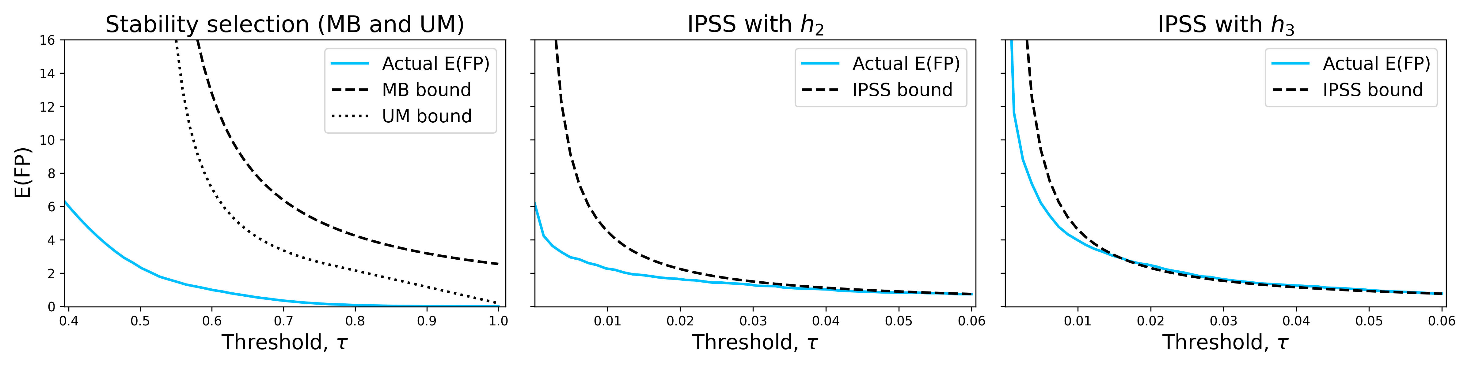
Figure 3. Bounds on $\mathrm{E(FP)}$ as a function of $\tau$. Results are averaged over $100$ data sets simulated from an independent linear regression model as described in Section 1, with $n=200$, $p=1000$, $s=8$, and $\mathrm{SNR}=1$. (Left) The MB and UM bounds (Equations 4.8 and 4.9) and the actual $\mathrm{E(FP)}$ for stability selection. Here, $q_{*}$ is set to $50$ following Shah and Samworth (2013, Figure 2). (Middle) The IPSS bound using $h_{2}$ (Equation 4.4) and the actual $\mathrm{E(FP)}$. (Right) The IPSS bound using $h_{3}$ (Equation 4.5) and the actual $\mathrm{E(FP)}$.

The $r$-concave bound. Shah and Samworth (2013) present another upper bound on $\mathrm{E(FP)}$ under assumptions based on the notion of $r$-concavity. While tighter than the MB and UM bounds, this bound is more involved, requiring several assumptions that are justified empirically rather than with proof. In addition to being obtained via heuristic arguments, it does not have a closed form and hence must be approximated with another algorithm. This lack of closed form also makes the $r$-concave bound difficult to compare with Equations 4.2, 4.8, and 4.9. Finally, in practice, stability selection with the $r$-concave bound does not significantly outperform stability selection with the UM bound (Hofner et al., 2015), especially not to the extent that IPSS does below. We therefore only consider stability selection with the MB and UM bounds in what follows.

5.  Simulations

We present empirical results from simulations with linear regression and logistic regression for a variety of feature distributions. We compare the performance of IPSS and the stability selection methods of Meinshausen and Bühlmann (2010) and Shah and Samworth (2013), as well as lasso.

Setup. We generate simulated data from three models: linear regression with normal residuals, where

$$Y_{i} =\beta^{\mathtt{T}}X_{i}+\epsilon_{i},\quad\epsilon_{i}\sim\mathcal{N}(0,\sigma^{2}),$$

linear regression with residuals from a Student’s $t$ distribution with $2$ degrees of freedom,

$$Y_{i} =\beta^{\mathtt{T}}X_{i}+\epsilon_{i},\quad\epsilon_{i}\sim t(2),$$

and binary logistic regression, where

$$Y_{i} \sim\mathrm{Bernoulli}(p_{i}),\quad p_{i}=\frac{\exp(\gamma\beta^{\mathtt{T}}X_{i})}{1+\exp(\gamma\beta^{\mathtt{T}}X_{i})},$$

for $i\in\{1,\ldots,n\}$. For each simulated data set, the coefficient vector $\beta$ has $s$ nonzero entries located at randomly chosen coordinates in $\{1,\dots,p\}$, where $s=10$ or $s=20$. Half of the entries are evenly spaced between $-1$ and $-0.5$, and the other half are evenly spaced between $0.5$ and $1$. We simulate features using the following designs; these are similar to some of the experimental designs used by Meinshausen and Bühlmann (2010, Section 4). In all cases, $X_{i}$ is independent of $\epsilon_{i}$, and $(X_{1},Y_{1}),\ldots,(X_{n},Y_{n})$ are independent and identically distributed.

• Independent: $X_{i}\sim\mathcal{N}(0,I_{p})$ for all $i$, where $I_{p}$ is the $p\times p$ identity matrix.

• Toeplitz: $X_{i}\sim\mathcal{N}(0,\Sigma)$ where $\Sigma_{ij}=\rho^{\lvert i-j\rvert}$. We consider two cases: $\rho=0.5$ and $\rho=0.9$.

• Factor model: $X_{i}=\sum_{k=1}^{K}f_{ik}\varphi_{k}+\eta_{i}$ where $f_{ik},\varphi_{k},\eta_{i}\sim\mathcal{N}(0,1)$ independently for all $i$, $k$.

• Prostate cancer, RPPA: $X_{i}\sim\mathcal{N}(0,\Sigma)$ where $\Sigma$ is the estimated covariance matrix of Reverse Phase Protein Array (RPPA) data from prostate cancer patients (Vasaikar et al., 2018).

• Prostate cancer, miRNA: Same as above but for MicroRNA data from the same cohort.

For each feature $j\in\{1,\dots,p\}$, $(X_{1j},\ldots,X_{nj})$ is standardized to have mean $0$ and variance $1$. In the case of linear regression, the responses $Y_{1},\ldots,Y_{n}$ are centered to have mean $0$. For linear regression with normal residuals, $\sigma^{2}$ is chosen to satisfy a specified signal-to-noise ratio (SNR), defined as $\mathrm{SNR}=\mathrm{Var}(\beta^{\mathtt{T}}X_{i})/\sigma^{2}$ and empirically estimated by $\mathrm{SNR}\approx\sum_{i=1}^{n}(\beta^{\mathtt{T}}X_{i})^{2}/(n\sigma^{2})$ where $\beta$ is generated as above and $X_{i}$ is a random vector distributed according to one of the listed designs. For logistic regression, the parameter $\gamma>0$ determines the strength of the signal.

Each experimental setting is determined by the choice of model, design, $n$, $p$, $s$, and SNR (for linear regression with normal residuals) or $\gamma$ (for logistic regression). For each setting we perform $100$ trials, where one trial consists of generating a data set, estimating the selection probabilities via Algorithm 1 with $B=50$ subsamples, and choosing features according to each criterion. For linear regression, the baseline feature selection algorithm $\hat{S}_{\lambda}$ is lasso. For logistic regression, $\hat{S}_{\lambda}$ is $L^{1}$-regularized logistic regression (Lee et al., 2006).

Measures of performance. We quantify performance using the number of true positives (TP) and the number of false positives (FP). In each case, a selected feature is a true positive if its corresponding $\beta$ entry is nonzero, and is a false positive otherwise. As in Section 1, the black dotted line in each FP plot shows the target value of $\mathrm{E(FP)}$. A tight bound on $\mathrm{E(FP)}$ should lead to curves lying close to this line. This is because implementations of all the stability selection algorithms and IPSS involve replacing the inequalities in their respective $\mathrm{E(FP)}$ bounds with equalities in order to determine parameters. For example, if one specifies a target $\mathrm{E(FP)}$ of $2$, then a perfectly calibrated algorithm would produce an actual $\mathrm{E(FP)}$ of $2$.

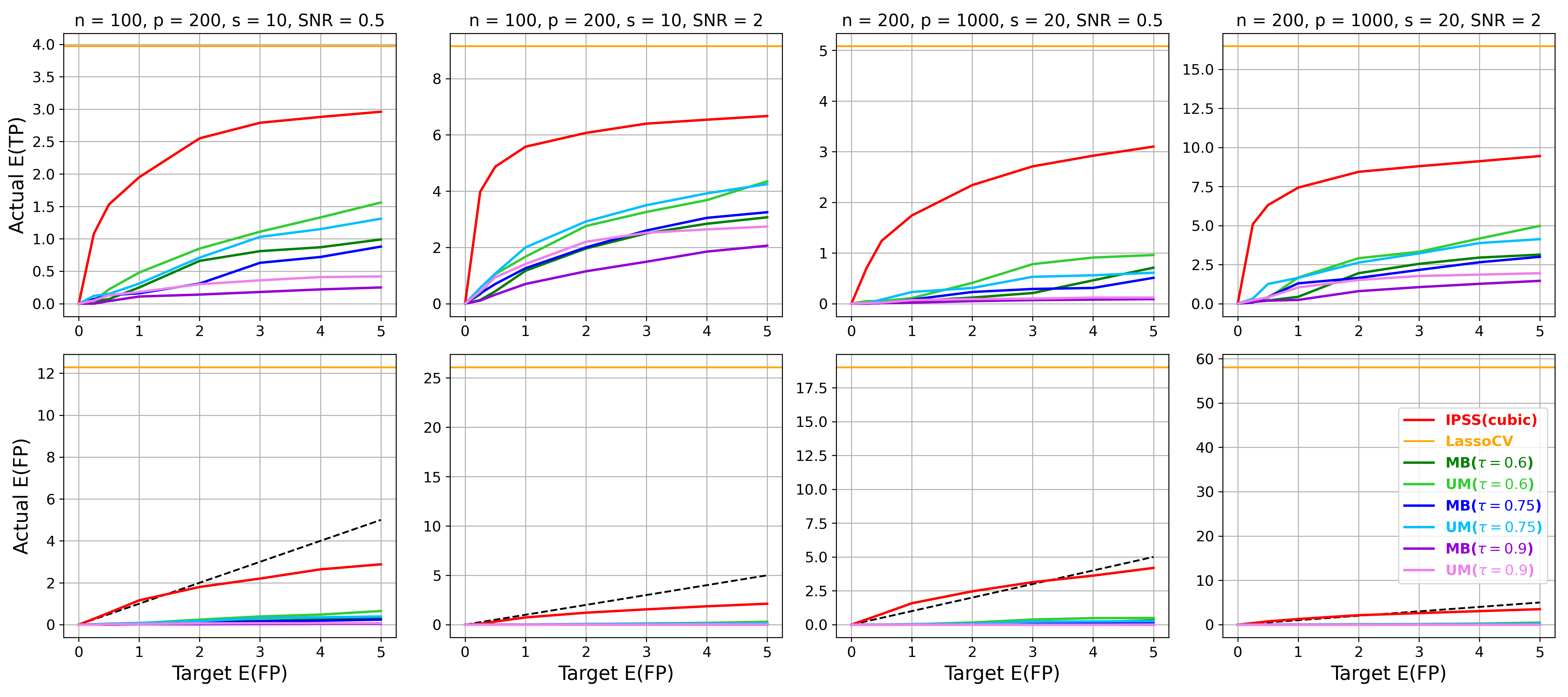
Figure 4. Linear regression with normal residuals and independent design.

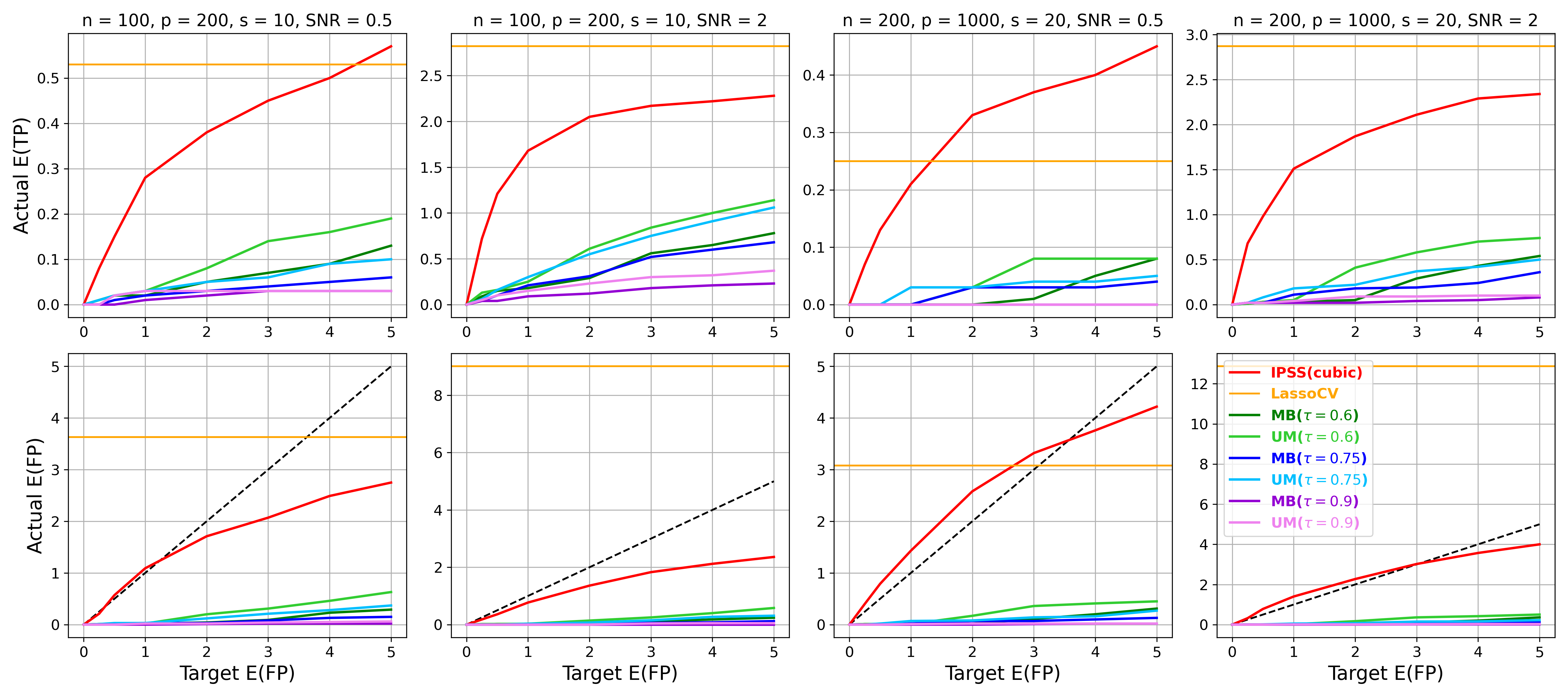
Figure 5. Linear regression with $t$ residuals and independent design.

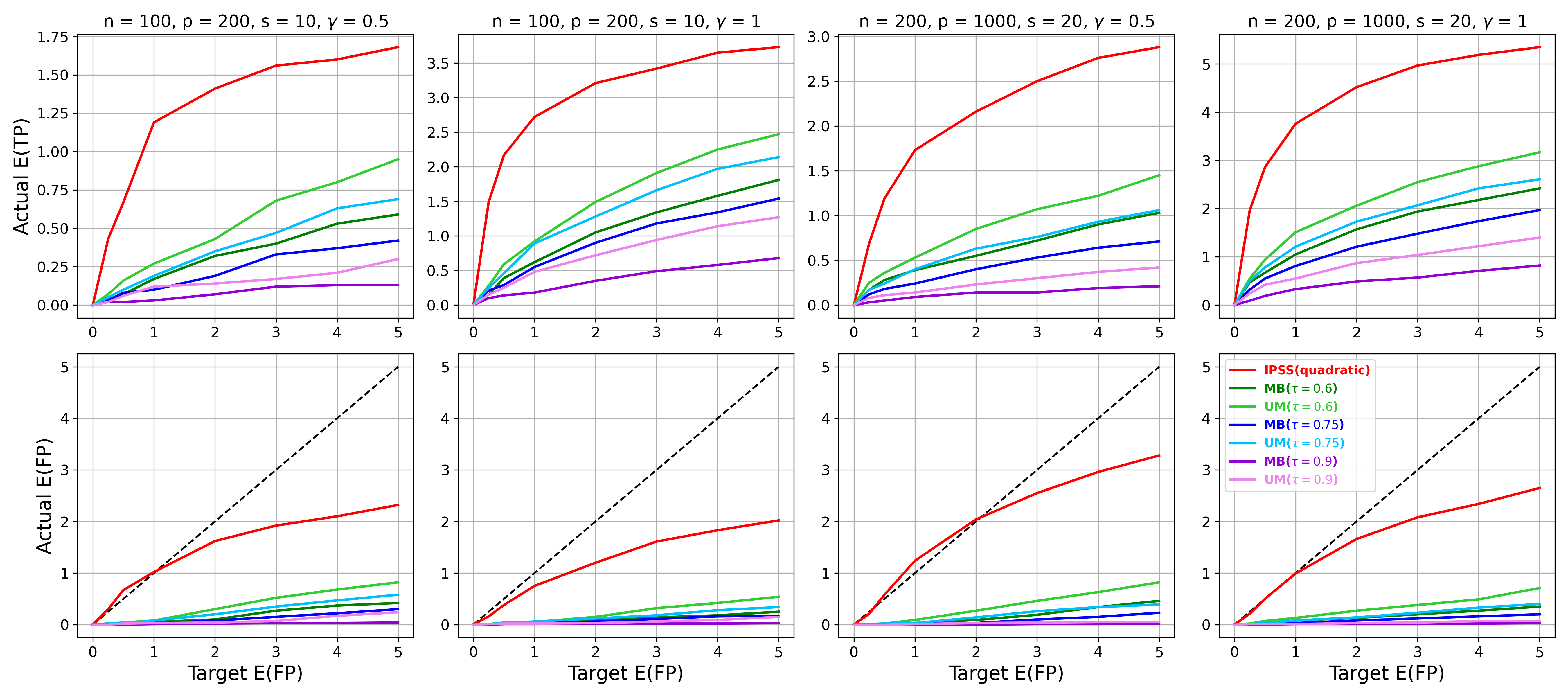
Figure 6. Logistic regression with independent design.

Results. Figures 4, 5, and 6 show the results for the independent design experiments; see Section S4.2 for the rest of the results. In all simulations, both here and in Section S4.2, IPSS yields an actual $\mathrm{E(FP)}$ closer to the target $\mathrm{E(FP)}$ than either MB or UM with any $\tau\in\{0.6,0.75,0.9\}$. This is due to the strength of the IPSS bound on $\mathrm{E(FP)}$ relative to those for MB and UM; see Section 4.3. Moreover, the average number of true positives (actual $\mathrm{E(TP)}$) is higher for IPSS than for MB or UM in all cases, often substantially so. Lasso with cross-validation (LassoCV) tends to have a relatively high $\mathrm{E(TP)}$ at the expense of an exceedingly high $\mathrm{E(FP)}$. This tendency was so pronounced for logistic regression that the IPSS and stability selection results were difficult to see when put on the same plot as LassoCV, which is why LassoCV is not shown in the logistic regression plots.

These results indicate that IPSS provides a better balance between true and false positives in a wide range of settings than both stability selection and LassoCV. That is, while stability selection (MB and UM) has low FP at the expense of low TP, and LassoCV has high TP at the expense of high FP, IPSS get closer to the user-specified $\mathrm{E(FP)}$, while achieving moderate-to-high TP that can even approach the TP of LassoCV. For example, in the second column in Figure 4 at a target $\mathrm{E(FP)}$ of $1$, the best stability selection method has $\mathrm{E(FP)}\approx 0$ and $\mathrm{E(TP)}\approx 2$, LassoCV has $\mathrm{E(FP)}\approx 26$ and $\mathrm{E(TP)}\approx 9$, whereas IPSS has $\mathrm{E(FP)}\approx 1$ and $\mathrm{E(TP)}\approx 6$.

6.  Applications

6.1.  Prostate cancer.

We applied IPSS, MB, and UM to the expression levels of $p=125$ genes in $n=348$ prostate cancer patients using RPPA data (Vasaikar et al., 2018). The response is tumor purity—the proportion of cancerous cells in a tissue sample—and the goal is to identify the genes that are most related to tumor purity. Since tumor purity takes values in $[0,1]$, we use lasso as our baseline selection algorithm. For MB and UM, we set $\tau=0.75$, for IPSS we use $h_{3}$, and the target $\mathrm{E(FP)}$ is $1$ for all three methods. Figure 7 shows the results. Although it is difficult to know which features should be selected on real data such as this, a literature search overwhelming supports the claim that all $10$ genes identified by IPSS play a nontrivial role in prostate cancer. For brevity, we list just one publication per gene: BAK1 (Shi et al., 2007), DIRAS3 (Sutton et al., 2019), MAPK9 (Rodríguez-Berriguete et al., 2012), STK11 (Grossi et al., 2015), NOTCH1 (Rice et al., 2019), PKC (Tanaka et al., 2003), PTEN (Jamaspishvili et al., 2018), SMAD1 (Qiu et al., 2007), EIF4E (D’Abronzo and Ghosh, 2018), and SQSTM1 (Huang et al., 2018).

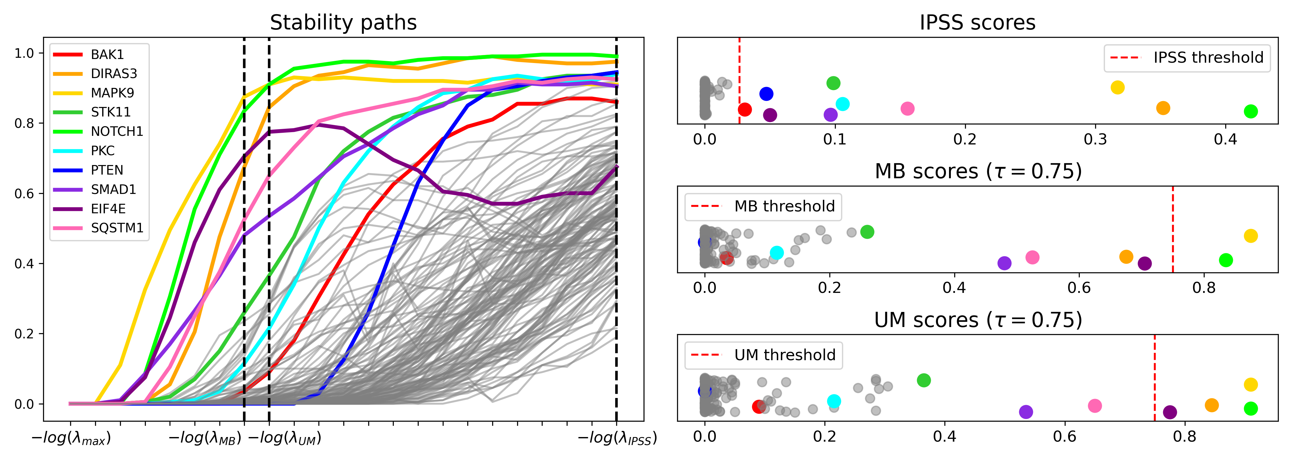
Figure 7. Prostate cancer results. (Left) Estimated stability paths for each gene in the prostate cancer data set. The horizontal axis is on a log scale, with dashed lines at $-\log(\lambda_{\mathrm{MB}})$, $-\log(\lambda_{\mathrm{UM}})$, and $-\log(\lambda_{\mathrm{IPSS}})$. As in Figure 2, $\lambda_{\mathrm{MB}}$ and $\lambda_{\mathrm{UM}}$ are significantly larger than $\lambda_{\mathrm{IPSS}}$, causing stability selection to miss important information that IPSS successfully captures. For example, the selection probability for PTEN is essentially zero between $\lambda_{\mathrm{max}}$ and $\lambda_{\mathrm{UM}}$, but is approximately $0.9$ at $\lambda_{\mathrm{IPSS}}$. (Right) Feature scores for IPSS (top), MB (middle), and UM (bottom), along with their respective thresholds (vertical red lines) separating selected and unselected genes. Scores are one-dimensional and correspond to the horizontal axes. Genes selected by at least one method are shown in color, and the rest are in gray. MB selects $2$ genes, UM selects $4$, and IPSS selects $10$.

6.2.  Colon cancer.

We applied IPSS, MB, and UM to the expression levels of $p=1908$ genes in $n=62$ tissue samples, $40$ cancerous and $22$ normal (Alon et al., 1999). The goal is to identify genes whose expression levels differ between the cancerous and normal samples. The threshold for MB and UM is $\tau=0.6$, for IPSS we use $h_{2}$, and for all three methods, we use $L^{1}$-regularized logistic regression with a target $\mathrm{E(FP)}$ of $1$. Expression levels are log-transformed and standardized as in Shah and Samworth (2013, Section 4.2), where these data are also studied in the context of stability selection. Figures 8 and 9 show the results. We again find that the IPSS results are corroborated by the literature; genes are identified by their GenBank accession numbers and, when available, official symbols (in parentheses): H06524 (Chen et al., 2017), H08393, J02854 (MYL9), M26383 (IL-1), R87126, and T47377 (S-100) (Wang et al., 2010), J05032 (DARS1) (Shu et al., 2024), M36634 (VIP) (Levy et al., 2002), M63391 (desmin) (Arentz et al., 2011), R36977 (GTF3A) (Anuraga et al., 2021), R54097 (EIF2S2) (Zhang et al., 2020), X12671 (hnRNP A1) (Ushigome et al., 2005), X63629 (P-cadherin) (Sun et al., 2011), Z50753 (GUCA2B) (Nomiri et al., 2022).

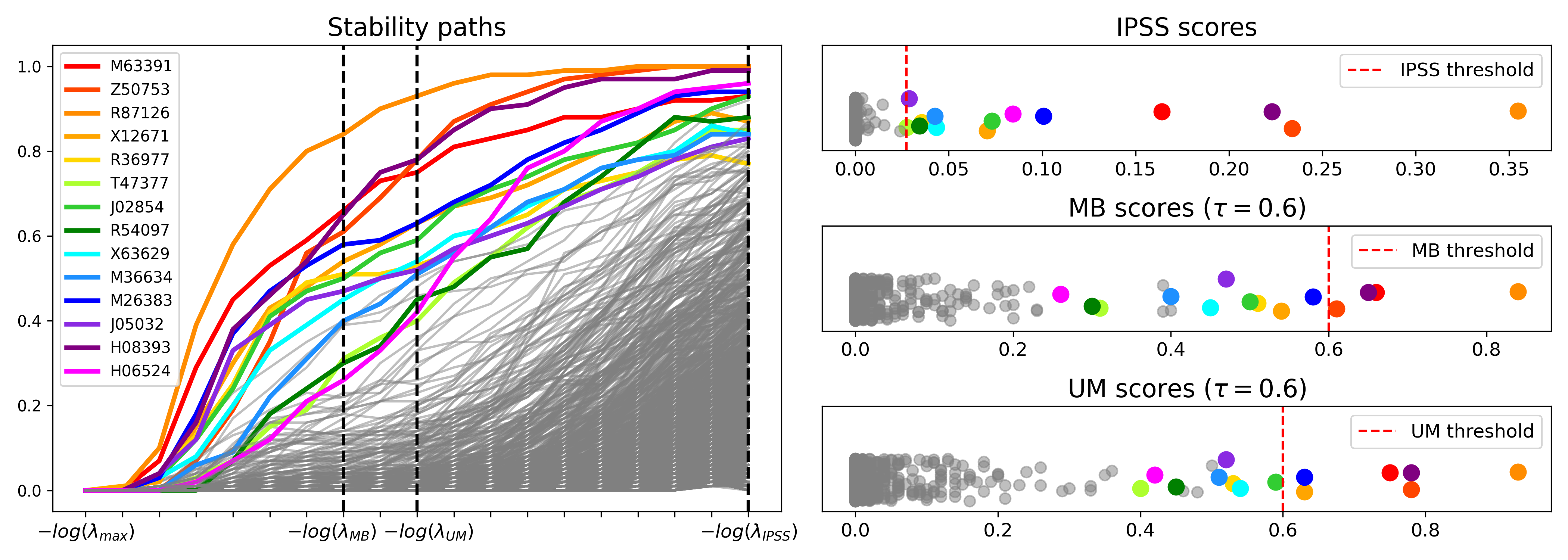
Figure 8. Colon cancer results. (Left) Estimated stability paths for each gene in the colon cancer data set. Dashed lines at $-\log(\lambda_{\mathrm{MB}})$, $-\log(\lambda_{\mathrm{UM}})$, and $-\log(\lambda_{\mathrm{IPSS}})$. (Right) Feature scores for IPSS (top), MB (middle), and UM (bottom), along with their respective thresholds (vertical red lines) separating selected and unselected features. Genes selected by at least one method are shown in color, and the rest are in gray. MB selects $4$ genes, UM selects $6$, and IPSS selects $14$.

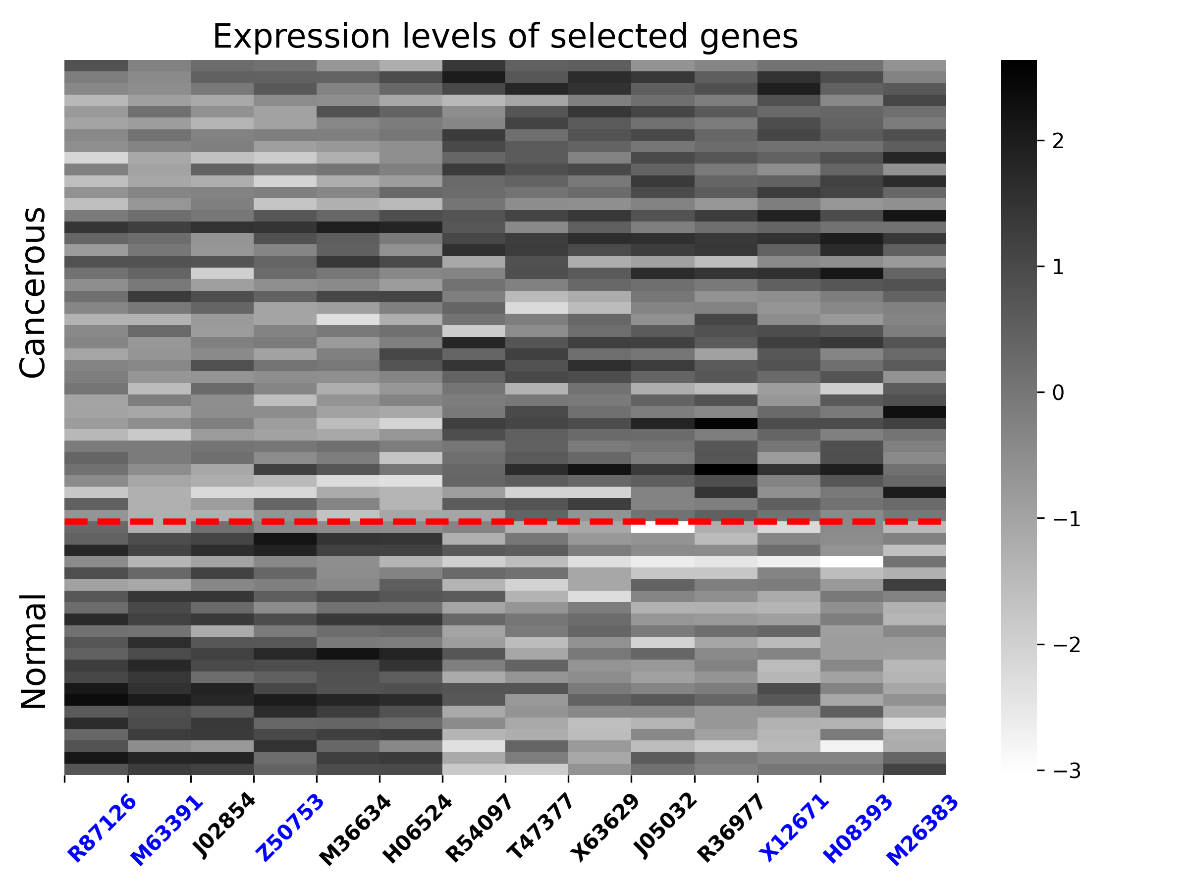
Figure 9. Expression level heatmap for the $13$ genes selected by IPSS. Each of the $62$ rows corresponds to one tissue sample. The first $40$ rows are cancerous, and the latter $22$ rows are normal; the dashed red line separates the two classes. Each column corresponds to a gene selected by IPSS. Blue text indicates genes also selected by UM. The bar on the right shows expression intensity levels. For each gene, there is a clear distinction between expression levels for cancer versus normal samples.

7.  Discussion

IPSS has several attractive properties. It has stronger theoretical guarantees than stability selection, and yields significantly better performance on a wide range of simulated and real data. It has the same computational cost as stability selection and is easier to tune, requiring only the target $\mathrm{E(FP)}$ to be specified. IPSS is also very flexible, allowing for any choice of function $f$ and probability measure $\mu$. In this work, we focused on the functions $h_{2}$ and $h_{3}$ and the measure $\mu_{1}$ due to their favorable theoretical properties and empirical performance. However, it is possible that other functions and measures will lead to better results; investigating this point is an interesting line of future work.

Another interesting direction is to apply IPSS to other feature selection algorithms, such as graphical lasso, elastic net, and adaptive lasso (Friedman et al., 2008; Zou and Hastie, 2005; Zou, 2006). In the case of elastic net, there are two regularization parameters, and while our methodology and theory appears to carry over to this setting (now with $\Lambda\subseteq(0,\infty)^{2}$ and $(\lambda_{1},\lambda_{2})\mapsto\hat{S}_{\lambda_{1},\lambda_{2}}$), it remains to work out the details and investigate the performance of IPSS in the context of multiple regularization parameters. Finally, we noted in Section 3 that stability selection is often used in conjunction with other statistical methods. Given that IPSS yields better results than stability selection at no additional cost and with less tuning, it would be interesting to study these joint methods with IPSS in place of stability selection.

Data availability and code

The prostate cancer data set used in this work is freely available at https://www.linkedomics.org/data_download/TCGA-PRAD. The colon cancer data set is freely available at http://genomics-pubs.princeton.edu/oncology/affydata/index.html. Both data sets, along with code from this work, are also freely available at https://github.com/omelikechi/ipss.

Supplementary material for “Integrated path stability selection”

We provide further details on the implementation of IPSS (Section S1), prove Theorems 4.1 and 4.2 (Section S2), state and prove results for IPSS with functions that are not considered in the main text (Section S3), and provide additional empirical results (Section S4).

S1.  Algorithmic details

In Section S1.1, we elaborate on the construction of $\Lambda_{\mathrm{IPSS}}$. In Section S1.2, we describe a simple way to approximate the integrals in the IPSS criterion (Equation 2.4) for a wide range of functions $f$ and measures $\mu$.

S1.1.  Construction of $\bm{\Lambda_{\mathrm{IPSS}}}$.

Features are always standardized to have mean $0$ and standard deviation $1$ in both linear and logistic regression, and the response is always centered to have mean $0$ in linear regression. For lasso, the upper endpoint $\lambda_{\mathrm{max}}$ of $\Lambda_{\mathrm{IPSS}}$ is set to twice the maximum correlation between the features and response; that is, $\lambda_{\mathrm{max}}=2\max_{j}\lvert\frac{1}{n}\sum_{i=1}^{n}x_{ij}y_{i}\rvert$. For $L^{1}$-regularized logistic regression, $\lambda_{\mathrm{max}}=5/\max_{j}\lvert\frac{1}{n}\sum_{i=1}^{n}x_{ij}\widetilde{y}_{i}\rvert$ where $\widetilde{y}_{i}=y_{i}-\bar{y}(1-\bar{y})$ and $\bar{y}=\tfrac{1}{n}\sum_{i=1}^{n}y_{i}$. Both constructions ensure all features have selection probability close to zero at $\lambda_{\mathrm{max}}$. For other regularized feature selection algorithms, $\lambda_{\mathrm{max}}$ can be chosen via grid search.

Next, we define $\lambda_{\mathrm{min}}$ by starting at $\lambda=\lambda_{\mathrm{max}}$ and decreasing $\lambda$ over a grid of $100$ points that are evenly spaced on a log scale between $\lambda_{\mathrm{max}}/10^{10}$ and $\lambda_{\mathrm{max}}$, stopping once $\hat{S}_{\lambda}(Z_{1:n})$ selects more than $p/2$ features. We then set $\lambda_{\mathrm{min}}$ to be the smallest value of $\lambda$ in this grid such that fewer than $p/2$ features were selected. The idea is that we wish to quickly identify a reasonable lower endpoint that is not so close to $\lambda_{\mathrm{max}}$ that the selection paths are cut off prematurely, but not so small that nearly all of the $p$ features are selected, since exceedingly small regularization values can cause unnecessary computational difficulties. Our experience suggests that $p/2$ is an effective value for the maximum number of features selected and that results are insensitive to this choice.

Finally, $\lambda_{\mathrm{IPSS}}$ is chosen as follows. Given the integral cutoff value $C>0$, recall that

$$\lambda_{\mathrm{IPSS}} =\inf\big{\{}\lambda\in(0,\lambda_{\mathrm{max}}):\mathcal{I}(\lambda,\lambda_{\mathrm{max}})\leq C\big{\}}$$

according to Equation 2.6 in the main text, where $\mathcal{I}$ is an integral over $[\lambda,\lambda_{\mathrm{max}}]$. In practice, to approximate the infimum, we partition $\Lambda=[\lambda_{\mathrm{min}},\lambda_{\mathrm{max}}]$ into a grid of $r$ points evenly spaced on a log scale. We successively add the integrand of $\mathcal{I}$ evaluated at each value of $\lambda$ in the grid, starting from $\lambda_{\mathrm{max}}$ and stopping either when $\lambda=\lambda_{\mathrm{min}}$ or when the sum surpasses $C$, whichever comes first. In the latter case, $\lambda_{\mathrm{IPSS}}$ is the smallest $\lambda$ in the grid such that the corresponding Riemann sum in S1.1 is at most $C$.

S1.2.  Numerical approximation of the IPSS integral.

To implement IPSS, one must approximate the integral in Equation 2.4. We use a simple numerical approximation based on a Riemann sum, described in S1.1. Consider the class of probability measures $\mu_{\alpha}(d\lambda)=z^{-1}_{\alpha}\lambda^{-\alpha}d\lambda$ on $\Lambda=[\lambda_{\mathrm{min}},\lambda_{\mathrm{max}}]\subseteq(0,\infty)$, where $\alpha\in\mathbb{R}$ and the normalizing constant $z_{\alpha}$ is

$$z_{\alpha} =\int_{\Lambda}\lambda^{-\alpha}d\lambda=\begin{cases}\log\big{(}\lambda_{\mathrm{max}}/\lambda_{\mathrm{min}}\big{)}&\text{if}\ \alpha=1\\[8.0pt] \frac{1}{1-\alpha}\big{(}\lambda_{\mathrm{max}}^{1-\alpha}-\lambda_{\mathrm{min}}^{1-\alpha}\big{)}&\text{if}\ \alpha\neq 1.\end{cases}$$

The parameter $\alpha$ controls the scale on which the $\lambda$ values are weighted. For instance, $\alpha=0$ and $\alpha=1$ correspond to linear and log scales, respectively. We find that $\mu_{1}$ is preferable to $\mu_{0}$ in terms of selection performance, and that results are similar for $\alpha\in[0.5,1.5]$, motivating our choice of $\mu_{1}$.

Proposition S1.1.

Fix $\alpha\in\mathbb{R}$, let $\Lambda=[\lambda_{\mathrm{min}},\lambda_{\mathrm{max}}]\subseteq(0,\infty)$, and define $\lambda_{k,r}=\lambda_{\mathrm{min}}^{1-k/r}\lambda_{\mathrm{max}}^{k/r}$ for all $r\in\mathbb{N}$, $k\in\{0,1,\dots,r\}$. For any Riemann integrable $g:\Lambda\to\mathbb{R}$,

$$\lim_{r\to\infty}\frac{1-(\lambda_{\mathrm{min}}/\lambda_{\mathrm{max}})^{1/r}}{z_{\alpha}}\sum_{k=1}^{r}\lambda_{k,r}^{1-\alpha}g(\lambda_{k,r}) =\int_{\Lambda}g(\lambda)\mu_{\alpha}(d\lambda).$$ (S1.1)

Proof.

Fix $m\in\mathbb{N}$. The sequence $\Lambda_{r}=(\lambda_{0,r},\lambda_{1,r},\dots,\lambda_{r,r})$ partitions $\Lambda$. Furthermore,

$$\lambda_{k,r}-\lambda_{k-1,r} =\Big{(}1-\big{(}\lambda_{\mathrm{min}}/\lambda_{\mathrm{max}}\big{)}^{1/r}\Big{)}\lambda_{k,r}$$ (S1.2)

for all $r$ and $k\in\{1,\dots,r\}$, and hence,

$$\max_{k}\big{\lvert}\lambda_{k,r}-\lambda_{k-1,r}\big{\rvert}\leq\Big{\lvert}1-\big{(}\lambda_{\mathrm{min}}/\lambda_{\mathrm{max}}\big{)}^{1/r}\Big{\rvert}|\lambda_{\mathrm{max}}|\longrightarrow 0$$ (S1.3)

as $r\to\infty$. Therefore, Equations S1.2 and S1.3 imply that

$$\frac{1-(\lambda_{\mathrm{min}}/\lambda_{\mathrm{max}})^{1/r}}{z_{\alpha}}\sum_{k=1}^{r}\lambda_{k,r}^{1-\alpha}g(\lambda_{k,r}) =\frac{1}{z_{\alpha}}\sum_{k=1}^{r}\lambda_{k,r}^{-\alpha}g(\lambda_{k,r})(\lambda_{k,r}-\lambda_{k-1,r})\longrightarrow\int_{\Lambda}g(\lambda)\mu_{\alpha}(d\lambda)$$

as $r\to\infty$ since $\lambda^{-\alpha}g(\lambda)$ is Riemann integrable on $\Lambda$. ∎

If $\alpha=1$ then $\lambda^{1-\alpha}_{k,r}=1$ for all $k$ and $r$. Thus, when using our recommended choices of $f=h_{m}$ and $\mu=\mu_{1}$, computation of the IPSS criterion (Equation 2.4) amounts to

$$\int_{\Lambda}f(\hat{\pi}_{j}(\lambda))\mu(d\lambda)=\int_{\Lambda}h_{m}(\hat{\pi}_{j}(\lambda))\mu_{1}(d\lambda) \approx\frac{1-(\lambda_{\mathrm{min}}/\lambda_{\mathrm{max}})^{1/r}}{z_{1}}\sum_{k=1}^{r}h_{m}(\hat{\pi}_{j}(\lambda_{k,r}))$$ (S1.4)

by applying S1.1 with $\alpha=1$ and $g(\lambda)=h_{m}(\hat{\pi}_{j}(\lambda))$. Furthermore, $h_{m}$ is a simple function of the estimated selection probabilities, making Equation S1.4 very inexpensive to compute once the estimated selection probabilities are obtained.

The use of S1.1 for IPSS is justified by S1.2, which gives general conditions for functions of the form $\lambda\mapsto f(\hat{\pi}_{j}(\lambda))$ to be Riemann integrable when $\hat{S}_{\lambda}=\{j:\hat{\beta}_{j}(\lambda)\neq 0\}$ for some $\hat{\beta}_{j}:\Lambda\to\mathbb{R}$. In particular, $h_{m}\circ\hat{\pi}_{j}$ is Riemann integrable when using lasso since $h_{m}$ is continuous and lasso regularization paths $\lambda\mapsto\hat{\beta}_{j}(\lambda)$ are continuous whenever no two features are perfectly correlated (Mairal and Yu, 2012). More generally, it follows from the proof of S1.2 that Riemann integrability of $h_{m}\circ\hat{\pi}_{j}$ is implied by Riemann integrability of the indicators $\operatorname{\mathds{1}}(j\in\hat{S}_{\lambda})$.

Proposition S1.2.

Let $\Lambda$ be a closed interval in $\mathbb{R}$. Suppose $\hat{S}_{\lambda}$ is given by $\hat{S}_{\lambda}=\{j:\hat{\beta}_{j}(\lambda)\neq 0\}$ and that $\lambda\mapsto\hat{\beta}_{j}(\lambda)$ is continuous on $\Lambda$ for all $j\in\{1,\dots,p\}$. Then for every continuous function $f:[0,1]\to\mathbb{R}$, the composition $\lambda\mapsto f(\hat{\pi}_{j}(\lambda))$ is Riemann integrable.

Proof.

Fix $j\in\{1,\dots,p\}$. We first prove $\lambda\mapsto\operatorname{\mathds{1}}(j\in\hat{S}_{\lambda})$ is Riemann integrable. Since a bounded function on a closed interval is Riemann integrable if and only if it is continuous almost everywhere, it suffices to show $\lambda\mapsto\operatorname{\mathds{1}}(j\in\hat{S}_{\lambda})$ is continuous almost everywhere. To this end, we have

$$\operatorname{\mathds{1}}(j\in\hat{S}_{\lambda}) =\operatorname{\mathds{1}}(\hat{\beta}_{j}(\lambda)\neq 0)=\operatorname{\mathds{1}}\!\big{(}\lambda\in\hat{\beta}_{j}^{-1}(\mathbb{R}\setminus\{0\})\big{)}.$$

Since $\hat{\beta}_{j}$ is continuous, $U=\hat{\beta}_{j}^{-1}(\mathbb{R}\setminus\{0\})$ is an open subset of $\mathbb{R}$. A classical result from analysis states that every open subset of $\mathbb{R}$ is a countable union of disjoint open intervals. Letting $U=\bigcup_{k=1}^{\infty}(a_{k},b_{k})$ be such a union, we have

$$\operatorname{\mathds{1}}\!\big{(}\lambda\in\hat{\beta}_{j}^{-1}(\mathbb{R}\setminus\{0\})\big{)} =\operatorname{\mathds{1}}(\lambda\in U)=\operatorname{\mathds{1}}\!\big{(}\lambda\in{\textstyle\bigcup_{k=1}^{\infty}}(a_{k},b_{k})\big{)}.$$

Hence, $\operatorname{\mathds{1}}(j\in\hat{S}_{\lambda})=\operatorname{\mathds{1}}(\lambda\in\bigcup_{k=1}^{\infty}(a_{k},b_{k}))$, and it is clear from the latter expression that the set of discontinuities of $\operatorname{\mathds{1}}(j\in\hat{S}_{\lambda})$ is contained in $\bigcup_{k=1}^{\infty}\{a_{k},b_{k}\}$, which is countable and therefore has Lebesgue measure zero. Thus $\lambda\mapsto\operatorname{\mathds{1}}(j\in\hat{S}_{\lambda})$ is Riemann integrable, and it immediately follows that $\hat{\pi}_{j}$ is Riemann integrable since it is a linear combination of indicators of the form $\operatorname{\mathds{1}}(j\in\hat{S}_{\lambda})$.

To conclude the proof, we show that $f\circ\hat{\pi}_{j}:\Lambda\to\mathbb{R}$ is bounded and continuous almost everywhere (and hence Riemann integrable). Boundedness holds because $f$ is continuous on the compact set $[0,1]$. For the continuous almost everywhere claim, let $A$ and $B$ be the sets of discontinuities of $\hat{\pi}_{j}$ and $f\circ\hat{\pi}_{j}$, respectively. We know from the first part of the proof that $A$ has measure zero. Thus, it suffices to show $B\subseteq A$ or, equivalently, $A^{c}\subseteq B^{c}$. Fix $\lambda\in A^{c}$ and let $\lambda_{k}$ be any sequence in $\Lambda$ converging to $\lambda$. Then $y_{k}=\hat{\pi}_{j}(\lambda_{k})\to\hat{\pi}_{j}(\lambda)=y$ since $\hat{\pi}_{j}$ is continuous at $\lambda$. And since $f$ is continuous, $f(\hat{\pi}_{j}(\lambda_{k}))=f(y_{k})\to f(y)=f(\hat{\pi}_{j}(\lambda))$. Thus $\lambda\in B^{c}$ and hence $A^{c}\subseteq B^{c}$. ∎

S2.  Proofs

We begin by introducing some notation and preliminary results. Fix $B\geq 2$ throughout. For $\lambda>0$ and $j\in\{1,\dots,p\}$, define the simultaneous selection probability

$$\widetilde{\pi}_{j}(\lambda) =\frac{1}{B}\sum_{b=1}^{B}\operatorname{\mathds{1}}(j\in\hat{S}_{\lambda}(Z_{A_{2b-1}}))\operatorname{\mathds{1}}(j\in\hat{S}_{\lambda}(Z_{A_{2b}}))=\frac{1}{B}\sum_{b=1}^{B}U_{jb}(\lambda)$$

where $U_{jb}(\lambda)=\operatorname{\mathds{1}}(j\in\hat{S}_{\lambda}(Z_{A_{2b-1}}))\operatorname{\mathds{1}}(j\in\hat{S}_{\lambda}(Z_{A_{2b}}))$. Here, $\hat{S}_{\lambda}$ and $A_{2b-1},A_{2b}$ are defined as in Section 2. We use the following result (Equation S2.1), established in the proof of Shah and Samworth (2013, Lemma 1a): For all $\lambda>0$ and $j\in\{1,\dots,p\}$,

$$\hat{\pi}_{j}(\lambda)\leq\tfrac{1}{2}(1+\widetilde{\pi}_{j}(\lambda)).$$ (S2.1)

This holds since

$$0\leq\frac{1}{B}\sum_{b=1}^{B}\Big{(}1-\operatorname{\mathds{1}}(j\in\hat{S}_{\lambda}(Z_{A_{2b-1}}))\Big{)}\Big{(}1-\operatorname{\mathds{1}}(j\in\hat{S}_{\lambda}(Z_{A_{2b}}))\Big{)}=1-2\hat{\pi}_{j}(\lambda)+\widetilde{\pi}_{j}(\lambda).$$

The following lemma is used in the proof of Theorem 4.1; it is essentially an application of the multinomial theorem. For readability, let us define $\Delta_{m}=\big{\{}k\in\mathbb{Z}^{B}:k_{1},\ldots,k_{B}\geq 0,\,\sum_{b=1}^{B}k_{b}=m\big{\}}$, denote the multinomial coefficients by

$$\binom{m}{k_{1},\dots,k_{B}} =\frac{m!}{k_{1}!k_{2}!\cdots k_{B}!},$$

and define $N_{k}=\sum_{b=1}^{B}\operatorname{\mathds{1}}(k_{b}\neq 0)$ for $k\in\Delta_{m}$. Note that the assumed measurability of $\hat{S}_{\lambda}(Z_{A}):\Lambda\times\Omega\to 2^{\{1,\dots,p\}}$ implies measurability of $\widetilde{\pi}_{j}$, $\hat{\pi}_{j}$, and any continuous functions thereof.

Lemma S2.1.

Fix $m\in\mathbb{N}$. If Condition 1 holds for all $m^{\prime}\in\{1,\dots,m\}$, then for all $\lambda>0$,

$$\max_{j\in S^{c}}\,\mathrm{E}\big{(}\widetilde{\pi}_{j}(\lambda)^{m}\big{)} \leq\frac{1}{B^{m}}\sum_{k\in\Delta_{m}}\binom{m}{k_{1},\dots,k_{B}}(q(\lambda)/p)^{2N_{k}}.$$

Proof.

Fix $j\in S^{c}$ and define $0^{0}=1$. By the multinomial theorem,

$$\widetilde{\pi}_{j}(\lambda)^{m} =\frac{1}{B^{m}}\bigg{(}\sum_{b=1}^{B}U_{jb}(\lambda)\bigg{)}^{m}=\frac{1}{B^{m}}\sum_{k\in\Delta_{m}}\binom{m}{k_{1},\dots,k_{B}}\prod_{b=1}^{B}U_{jb}(\lambda)^{k_{b}}$$

$$=\frac{1}{B^{m}}\sum_{k\in\Delta_{m}}\binom{m}{k_{1},\dots,k_{B}}\prod_{b=1}^{B}U_{jb}(\lambda)^{\operatorname{\mathds{1}}(k_{b}\neq 0)}.$$

The last equality holds because $U_{jb}(\lambda)\in\{0,1\}$, and hence, $U_{jb}(\lambda)^{k_{b}}=U_{jb}(\lambda)$ whenever $k_{b}>0$. Next, since Condition 1 holds for all $m^{\prime}\leq m$ and since every $k\in\Delta_{m}$ has at most $m$ nonzero integers,

$$\mathbb{E}\prod_{b=1}^{B}U_{jb}(\lambda)^{\operatorname{\mathds{1}}(k_{b}\neq 0)} =\mathbb{P}\bigg{(}j\in\bigcap_{b:k_{b}\neq 0}\big{(}\hat{S}_{\lambda}(Z_{A_{2b-1}})\cap\hat{S}_{\lambda}(Z_{A_{2b}})\big{)}\bigg{)}\leq(q(\lambda)/p)^{2N_{k}}.$$

Therefore,

$$\mathrm{E}\big{(}\widetilde{\pi}_{j}(\lambda)^{m}\big{)} =\frac{1}{B^{m}}\sum_{k\in\Delta_{m}}\binom{m}{k_{1},\dots,k_{B}}\mathrm{E}\prod_{b=1}^{B}U_{jb}(\lambda)^{\operatorname{\mathds{1}}(k_{b}\neq 0)}$$

$$\leq\frac{1}{B^{m}}\sum_{k\in\Delta_{m}}\binom{m}{k_{1},\dots,k_{B}}(q(\lambda)/p)^{2N_{k}}.\qed$$

Proof of Theorem 4.1

Fix $\tau\in(0,1]$ and $m\in\mathbb{N}$. Suppressing $\lambda$ and $\Lambda$ to declutter the notation,

$$\mathbb{P}\big{(}j\in\hat{S}_{\mathrm{IPSS},h_{m}}\big{)} =\mathbb{P}\left(\int h_{m}(\hat{\pi}_{j})d\mu\geq\tau\right)\leq\mathbb{P}\left(\int h_{m}\big{(}\tfrac{1}{2}(1+\widetilde{\pi}_{j})\big{)}d\mu\geq\tau\right)=\mathbb{P}\left(\int\widetilde{\pi}_{j}^{m}d\mu\geq\tau\right)$$

$$\leq\frac{1}{\tau}\int\mathrm{E}(\widetilde{\pi}_{j}^{m})d\mu\leq\frac{1}{\tau B^{m}}\sum_{k\in\Delta_{m}}\binom{m}{k_{1},\dots,k_{B}}\int(q/p)^{2N_{k}}d\mu$$ (S2.2)

for all $j\in S^{c}$. The first inequality holds by Equation S2.1, namely $\hat{\pi}_{j}\leq\frac{1}{2}(1+\widetilde{\pi}_{j})$, and the fact that $h_{m}$ is monotonically increasing. The second equality holds since by the definition of $h_{m}$ in Equation 2.5, $h_{m}\big{(}\frac{1}{2}(1+x)\big{)}=x^{m}$ for $x\in[0,1]$. The second inequality is Markov’s inequality followed by exchanging the order of integration and expectation, which is justified by Tonelli’s theorem since $\widetilde{\pi}_{j}(\lambda)^{m}$ is nonnegative and measurable. The last inequality holds by Lemma S2.1. Thus,

$$\mathrm{E}\lvert\hat{S}_{\mathrm{IPSS},h_{m}}\cap S^{c}\rvert =\mathrm{E}\sum_{j=1}^{p}\operatorname{\mathds{1}}(j\in\hat{S}_{\mathrm{IPSS},h_{m}})\operatorname{\mathds{1}}(j\in S^{c})=\sum_{j=1}^{p}\mathbb{P}\big{(}j\in\hat{S}_{\mathrm{IPSS},h_{m}}\big{)}\operatorname{\mathds{1}}(j\in S^{c})$$

$$\leq\frac{1}{\tau B^{m}}\sum_{k\in\Delta_{m}}\binom{m}{k_{1},\dots,k_{B}}\int(q/p)^{2N_{k}}d\mu\sum_{j=1}^{p}\operatorname{\mathds{1}}(j\in S^{c})$$

$$\leq\frac{p}{\tau B^{m}}\sum_{k\in\Delta_{m}}\binom{m}{k_{1},\dots,k_{B}}\int(q/p)^{2N_{k}}d\mu.\qed$$

Proof of Theorem 4.2

In the notation of this section, Equation 4.2 becomes

$$\mathrm{E(FP)}\leq\frac{p}{\tau B^{m}}\sum_{k\in\Delta_{m}}\binom{m}{k_{1},\ldots,k_{B}}\int(q/p)^{2N_{k}}d\mu$$

where $q=q(\lambda)$. When $m=1$, each $k\in\Delta_{1}$ has a single nonzero entry $k_{b}=1$; thus, $|\Delta_{1}|=B$ and $N_{k}=1$ for all $k\in\Delta_{1}$. Therefore,

$$\mathrm{E(FP)}\leq\frac{p}{\tau B}\sum_{k\in\Delta_{1}}\binom{1}{k_{1},\dots,k_{B}}\int(q/p)^{2N_{k}}d\mu =\frac{p}{\tau B}\sum_{b=1}^{B}\int(q/p)^{2}d\mu=\frac{1}{\tau}\int\frac{q^{2}}{p}d\mu.$$

When $m=2$, there are $B$ elements $k\in\Delta_{2}$ with $N_{k}=1$ (each of which has $k_{b}=2$ for exactly one $b$), and $\binom{B}{2}$ elements $k\in\Delta_{2}$ with $N_{k}=2$ (each of which has $k_{b}=k_{b^{\prime}}=1$ for some $b\neq b^{\prime}$). Therefore,

$$\mathrm{E(FP)}\leq\frac{p}{\tau B^{2}}\sum_{k\in\Delta_{2}}\binom{2}{k_{1},\dots,k_{B}}\int(q/p)^{2N_{k}}d\mu =\frac{1}{\tau B^{2}}\int\bigg{(}\frac{Bq^{2}}{p}+\frac{B(B-1)q^{4}}{p^{3}}\bigg{)}d\mu.$$

When $m=3$, there are $B$ elements $k\in\Delta_{3}$ with $N_{k}=1$ (each of which has $k_{b}=3$ for one $b$), there are $2\binom{B}{2}$ elements $k\in\Delta_{3}$ with $N_{k}=2$ (having $k_{b}=2$ and $k_{b^{\prime}}=1$ for some $b\neq b^{\prime}$), and $\binom{B}{3}$ elements $k\in\Delta_{3}$ with $N_{k}=3$ (having $k_{b}=k_{b^{\prime}}=k_{b^{\prime\prime}}=1$ for some distinct $b,b^{\prime},b^{\prime\prime}$). Therefore,

$$\mathrm{E(FP)} \leq\frac{p}{\tau B^{3}}\sum_{k\in\Delta_{3}}\binom{3}{k_{1},\dots,k_{B}}\int(q/p)^{2N_{k}}d\mu$$

$$=\frac{1}{\tau B^{3}}\int\bigg{(}\frac{Bq^{2}}{p}+\frac{3B(B-1)q^{4}}{p^{3}}+\frac{B(B-1)(B-2)q^{6}}{p^{5}}\bigg{)}d\mu.\qed$$

S3.  IPSS with other functions

IPSS is very flexible in that one can choose essentially any $f$ and any $\mu$, the only technical restriction being that $f\circ\hat{\pi}_{j}\in L^{1}(\mu)$ for all $j\in\{1,\dots,p\}$. In this section, we provide results about IPSS for other choices of $f$. Throughout, we fix $\Lambda\subseteq(0,\infty)$ and a probability measure $\mu$ on $\Lambda$.

Our first result says that if a function $g$ dominates $f$, then the expected number of false positives selected by IPSS with $f$ is at most the expected number of false positives selected by IPSS with $g$. Similarly, the expected number of false negatives for IPSS with $g$ is at most the expected number of false negatives IPSS with $f$. We do not use Lemma S3.1 in this work, but it gives intuition for how IPSS depends on the choice of $f$, and could lead to useful bounds on functions not considered here.

Lemma S3.1.

Let $f$ and $g$ be functions from $[0,1]$ to $\mathbb{R}$. If $f\leq g$ then for all $\tau\in(0,1]$,

$$\mathrm{E}\lvert\hat{S}_{\mathrm{IPSS},f}\cap S^{c}\rvert\leq\mathrm{E}\lvert\hat{S}_{\mathrm{IPSS},g}\cap S^{c}\rvert\qquad\text{and}\qquad\mathrm{E}\lvert\hat{S}_{\mathrm{IPSS},g}^{c}\cap S\rvert\leq\mathrm{E}\lvert\hat{S}_{\mathrm{IPSS},f}^{c}\cap S\rvert.$$

Proof.

Fix $j\in\{1,\dots,p\}$ and $\tau\in(0,1]$. Since $f\leq g$,

$$\mathbb{P}(j\in\hat{S}_{\mathrm{IPSS},f}) =\mathbb{P}\left(\int f(\hat{\pi}_{j})d\mu\geq\tau\right)\leq\mathbb{P}\left(\int g(\hat{\pi}_{j})d\mu\geq\tau\right)=\mathbb{P}(j\in\hat{S}_{\mathrm{IPSS},g}).$$

Therefore,

$$\mathrm{E}\lvert\hat{S}_{\mathrm{IPSS},f}\cap S^{c}\rvert =\sum_{j=1}^{p}\mathbb{P}(j\in\hat{S}_{\mathrm{IPSS},f})\operatorname{\mathds{1}}(j\in S^{c})\leq\sum_{j=1}^{p}\mathbb{P}(j\in\hat{S}_{\mathrm{IPSS},g})\operatorname{\mathds{1}}(j\in S^{c})=\mathbb{E}\lvert\hat{S}_{\mathrm{IPSS},g}\cap S^{c}\rvert.$$

Similarly,

$$\mathrm{E}\lvert\hat{S}_{\mathrm{IPSS},g}^{c}\cap S\rvert =\sum_{j=1}^{p}\mathbb{P}(j\notin\hat{S}_{\mathrm{IPSS},g})\operatorname{\mathds{1}}(j\in S)=\sum_{j=1}^{p}(1-\mathbb{P}(j\in\hat{S}_{\mathrm{IPSS},g}))\operatorname{\mathds{1}}(j\in S)$$

$$\leq\sum_{j=1}^{p}(1-\mathbb{P}(j\in\hat{S}_{\mathrm{IPSS},f}))\operatorname{\mathds{1}}(j\in S)=\mathrm{E}\lvert\hat{S}_{\mathrm{IPSS},f}^{c}\cap S\rvert.\qed$$

S3.1.  Functions defined by monomials.

The functions $h_{m}$ defined in Equation 2.5 are zero on $[0,0.5]$. Another natural class of functions $\{w_{m}:m\in\mathbb{N}\}$ on $[0,1]$ is defined by

$$w_{m}(x) =x^{m}.$$

The $w$ stands for “whole,” indicating that these functions are positive on the whole unit interval. For example, TIGRESS (Haury et al., 2012) uses a special case of IPSS with $f=w_{1}$; see Section 3. Theorem S3.2 uses the following slight variation of Condition 1.

Condition 2.

We say Condition 2 holds for $m$ if for all $\lambda\in\Lambda$ and $\mathcal{B}\subseteq\{1,\dots,2B\}$ with $\lvert\mathcal{B}\rvert=m$,

$$\max_{j\in S^{c}}\,\mathbb{P}\bigg{(}j\in\bigcap_{b\in\mathcal{B}}\hat{S}_{\lambda}(Z_{A_{b}})\bigg{)} \leq(q(\lambda)/p)^{m}.$$

Theorem S3.2.

Let $\tau\in(0,1]$ and $m\in\mathbb{N}$. If Condition 2 holds for all $m^{\prime}\in\{1,\dots,m\}$, then

$$\mathrm{E}\lvert\hat{S}_{\mathrm{IPSS},w_{m}}\cap S^{c}\rvert \leq\frac{p}{\tau(2B)^{m}}\sum_{k_{1}+\cdots+k_{2B}=m}\binom{m}{k_{1},\dots,k_{2B}}\int_{\Lambda}(q(\lambda)/p)^{\sum_{b=1}^{2B}\operatorname{\mathds{1}}(k_{b}\neq 0)}\mu(d\lambda)$$

where $B$ is the number of subsampling steps in Algorithm 1 and the sum is over all nonnegative integers $k_{1},\ldots,k_{2B}$ such that $k_{1}+\cdots+k_{2B}=m$.

While Theorems 4.1 and S3.2 appear similar, there are two key differences. First, Theorem S3.2 has an additional factor of $2^{m}$ in the denominator, which is favorable in terms of tightness of the bound. On the other hand, the integrand in Theorem S3.2 is $(q(\lambda)/p)^{N_{k}}$ rather than $(q(\lambda)/p)^{2N_{k}}$ as in Theorem 4.1. Doubling the exponent makes the integral in Theorem 4.1 significantly smaller than the one in Theorem S3.2, since one typically has $q(\lambda)\ll p$ over much of $\Lambda$. This advantage outweighs the countervailing factor of $2^{m}$, which is why we recommend using $h_{m}$ in the main text.

Proof of Theorem S3.2..

Fix $\tau\in(0,1]$ and $m\in\mathbb{N}$. The proof is almost exactly the same as that of Theorem 4.1. Specifically, suppressing $\lambda$ and $\Lambda$ from the notation, the multinomial theorem gives

$$\hat{\pi}_{j}^{m} =\bigg{(}\frac{1}{2B}\sum_{b=1}^{2B}\operatorname{\mathds{1}}(j\in\hat{S}_{\lambda}(Z_{A_{b}}))\bigg{)}^{m}=\frac{1}{(2B)^{m}}\sum_{k_{1}+\cdots+k_{2B}=m}\binom{m}{k_{1},\dots,k_{2B}}\prod_{b\,:\,k_{b}\neq 0}\operatorname{\mathds{1}}(j\in\hat{S}_{\lambda}(Z_{A_{b}})).$$

Since Condition 2 holds for all $m^{\prime}\leq m$ and since at most $m$ of $k_{1},\ldots,k_{2B}$ are nonzero,

$$\mathrm{E}(\hat{\pi}_{j}^{m}) =\frac{1}{(2B)^{m}}\sum_{k_{1}+\cdots+k_{2B}=m}\binom{m}{k_{1},\dots,k_{2B}}\mathrm{E}\prod_{b\,:\,k_{b}\neq 0}\operatorname{\mathds{1}}(j\in\hat{S}_{\lambda}(Z_{A_{b}}))$$

$$\leq\frac{1}{(2B)^{m}}\sum_{k_{1}+\cdots+k_{2B}=m}\binom{m}{k_{1},\dots,k_{2B}}(q/p)^{N_{k}}$$

where $N_{k}=\sum_{b=1}^{2B}\operatorname{\mathds{1}}(k_{b}\neq 0)$. So for any $j\in\{1,\dots,p\}$, Markov’s inequality gives

$$\mathbb{P}(j\in\hat{S}_{\mathrm{IPSS},w_{m}}) =\mathbb{P}\left(\int w_{m}(\hat{\pi}_{j})d\mu\geq\tau\right)=\mathbb{P}\left(\int\hat{\pi}_{j}^{m}d\mu\geq\tau\right)\leq\frac{1}{\tau}\int\mathrm{E}(\hat{\pi}_{j}^{m})d\mu$$

$$\leq\frac{1}{\tau(2B)^{m}}\sum_{k_{1}+\cdots+k_{2B}=m}\binom{m}{k_{1},\dots,k_{2B}}\int(q/p)^{N_{k}}d\mu,$$

where Tonelli’s theorem justifies interchanging the order of expectation and integration. Therefore,

$$\mathbb{E}\lvert\hat{S}_{\mathrm{IPSS},w_{m}}\cap S^{c}\rvert =\sum_{j=1}^{p}\mathbb{P}(j\in\hat{S}_{\mathrm{IPSS},w_{m}})\operatorname{\mathds{1}}(j\in S^{c})$$

$$\leq\frac{1}{\tau(2B)^{m}}\sum_{k_{1}+\cdots+k_{2B}=m}\binom{m}{k_{1},\dots,k_{2B}}\int(q/p)^{N_{k}}d\mu\sum_{j=1}^{p}\operatorname{\mathds{1}}(j\in S^{c})$$

$$\leq\frac{p}{\tau(2B)^{m}}\sum_{k_{1}+\cdots+k_{2B}=m}\binom{m}{k_{1},\dots,k_{2B}}\int(q/p)^{N_{k}}d\mu.\qed$$

S3.2.  Some piecewise linear functions.

For $\delta\in[0,1)$ define $f_{\delta}:[0,1]\to[0,1]$ by

$$f_{\delta}(x) =\left(\frac{x-\delta}{1-\delta}\right)\operatorname{\mathds{1}}(x\geq\delta).$$

Note that $f_{\delta}$ is identically $0$ on $[0,\delta]$ and then rises linearly on $[\delta,1]$. Theorem S3.3 is a continuous analogue of Meinshausen and Bühlmann (2010, Theorem 1) when $\delta=0$.

Theorem S3.3.

Let $\delta\in[0,1)$, $\tau\in(0,1]$ such that $\tau>\tfrac{1-2\delta}{2(1-\delta)}$. If Condition 1 holds for $m=1$, then

$$\mathrm{E}\lvert\hat{S}_{\mathrm{IPSS},f_{\delta}}\cap S^{c}\rvert \leq\frac{1}{2(\tau-\tau\delta+\delta)-1}\int_{\Lambda}\frac{q(\lambda)^{2}}{p}\mu(d\lambda).$$

Proof.

Let $\delta\in[0,1)$ and $\tau\in(0,1]$ such that $\tau>(1-2\delta)/(2-2\delta)$. Fix $j\in S^{c}$. We have

$$\mathbb{P}(j\in\hat{S}_{\mathrm{IPSS},f_{\delta}}) =\mathbb{P}\left(\int f_{\delta}(\hat{\pi}_{j})d\mu\geq\tau\right)\leq\mathbb{P}\left(\frac{1}{1-\delta}\int\big{(}\tfrac{1}{2}(1+\widetilde{\pi}_{j})-\delta\big{)}\!\ d\mu\geq\tau\right)$$

$$=\mathbb{P}\left(\int\widetilde{\pi}_{j}\,d\mu\geq 2(\tau-\delta\tau+\delta)-1\right)\leq\frac{1}{2(\tau-\delta\tau+\delta)-1}\int\mathrm{E}(\widetilde{\pi}_{j})d\mu$$

$$\leq\frac{1}{2(\tau-\delta\tau+\delta)-1}\int(q/p)^{2}d\mu.$$

The first inequality holds since $f_{\delta}(\hat{\pi}_{j})\leq f_{\delta}\big{(}\frac{1}{2}(1+\widetilde{\pi}_{j})\big{)}=(\frac{1}{2}(1+\widetilde{\pi}_{j})-\delta)/(1-\delta)$ by Equation S2.1 and because $f_{\delta}$ is monotonically increasing with $f_{\delta}(x)=(x-\delta)/(1-\delta)$ for $x\geq 1/2$. The second inequality is by Markov’s inequality and Tonelli’s theorem. The final inequality follows from the definition of $\widetilde{\pi}_{j}$ and the assumption that Condition 1 holds for $m=1$. The assumption $\tau>(1-2\delta)/(2-2\delta)$ implies $2(\tau-\delta\tau+\delta)-1>0$, so the leading fraction is well-defined. Therefore,

$$\mathrm{E}\lvert\hat{S}_{\mathrm{IPSS},f_{\delta}}\cap S^{c}\rvert =\mathrm{E}\bigg{(}\sum_{j=1}^{p}\operatorname{\mathds{1}}(j\in\hat{S}_{\mathrm{IPSS},f_{\delta}})\operatorname{\mathds{1}}(j\in S^{c})\bigg{)}=\sum_{j=1}^{p}\mathbb{P}(j\in\hat{S}_{\mathrm{IPSS},f_{\delta}})\operatorname{\mathds{1}}(j\in S^{c})$$

$$\leq\frac{1}{2(\tau-\delta\tau+\delta)-1}\int\frac{q^{2}}{p^{2}}d\mu\sum_{j=1}^{p}\operatorname{\mathds{1}}(j\in S^{c})d\mu\leq\frac{1}{2(\tau-\delta\tau+\delta)-1}\int\frac{q^{2}}{p}d\mu.\qed$$

S4.  Additional empirical results

S4.1.  Empirical study of the theoretical conditions.

Our theory is based on Condition 1, which is less stringent than the exchangeability and not-worse-than-random-guessing conditions of Meinshausen and Bühlmann (2010); we refer to these as the MB conditions for short. However, even Condition 1 is unlikely to hold in general. For example, these conditions tend to be violated when true and non-true variables are highly correlated. Nonetheless, even then, empirically we find that only a small proportion of non-true features violate Condition 1 within the interval from $\lambda_{\mathrm{max}}$ to $\lambda_{\mathrm{IPSS}}$; see Figure S1. This also illustrates how our choice of $\lambda_{\mathrm{IPSS}}$ prevents IPSS from integrating over small regularization values where Condition 1 tends to fail.

Additionally, in Figure S1 we see that for any given value of $\lambda$, Condition 1 tends to be more likely to hold as $m$ increases. This subtle point contributes to the improved performance of IPSS with $h_{2}$ and $h_{3}$ relative to stability selection. Recall that the MB conditions imply Condition 1 holds for $m=1$. Hence, for any given $\lambda$, the more frequent violations of Condition 1 when $m=1$ imply that the MB conditions are more frequently violated, compared to Condition 1 for $m\in\{2,3\}$. Furthermore, while Equations 4.4 and 4.5 require Condition 1 to hold for $m\in\{1,2\}$ and $m\in\{1,2,3\}$, respectively, the $1/B$ and $1/B^{2}$ terms in their integrands mitigate the higher proportion of failures of Condition 1. This partly explains why Equations 4.4 and 4.5 hold in Figure 3 and why the target $\mathrm{E(FP)}$ is relatively well-approximated in all of our simulation results, even when Condition 1 does not necessarily hold for all features.

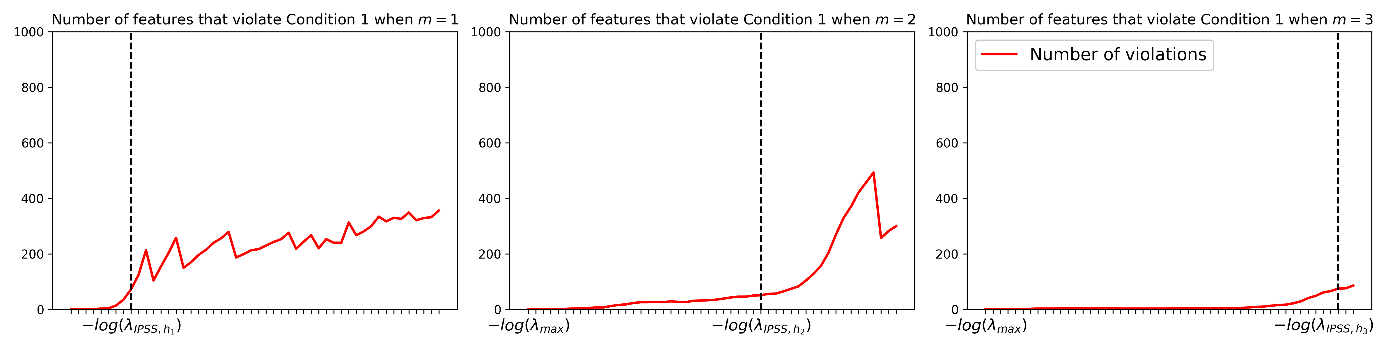
Figure S1. Violations of Condition 1 for highly correlated data. (Left) Number of features that violate Condition 1 when $m=1$ for each value of $\lambda$, with a dashed line at $-\log(\lambda_{\mathrm{IPSS},h_{m}})$. (Middle, Right) Same as the left plot but for $m=2$ and $3$, respectively. For all three plots, the horizontal axis is the same, on a log scale from $-\log(\lambda_{\mathrm{max}})$ to $-\log(\lambda_{\mathrm{min}})$. Data was generated using the linear regression model with normal residuals and Toeplitz design (see Section 5), with $n=200$, $p=1000$, $s=20$, $\mathrm{SNR}=1$, and $\rho=0.9$. The correlation parameter $\rho=0.9$ was selected to illustrate a worst-case scenario in which features are highly correlated.

S4.2.  Additional simulation study results.

This section contains additional results for other designs from the simulation study in Section 5. Figures S2, S3, S4, and S5 show results for linear regression with normal residuals. Figures S6, S7, and S8 show results for linear regression with $t$ residuals. Figures S9, S10, and S11 show results for logistic regression.

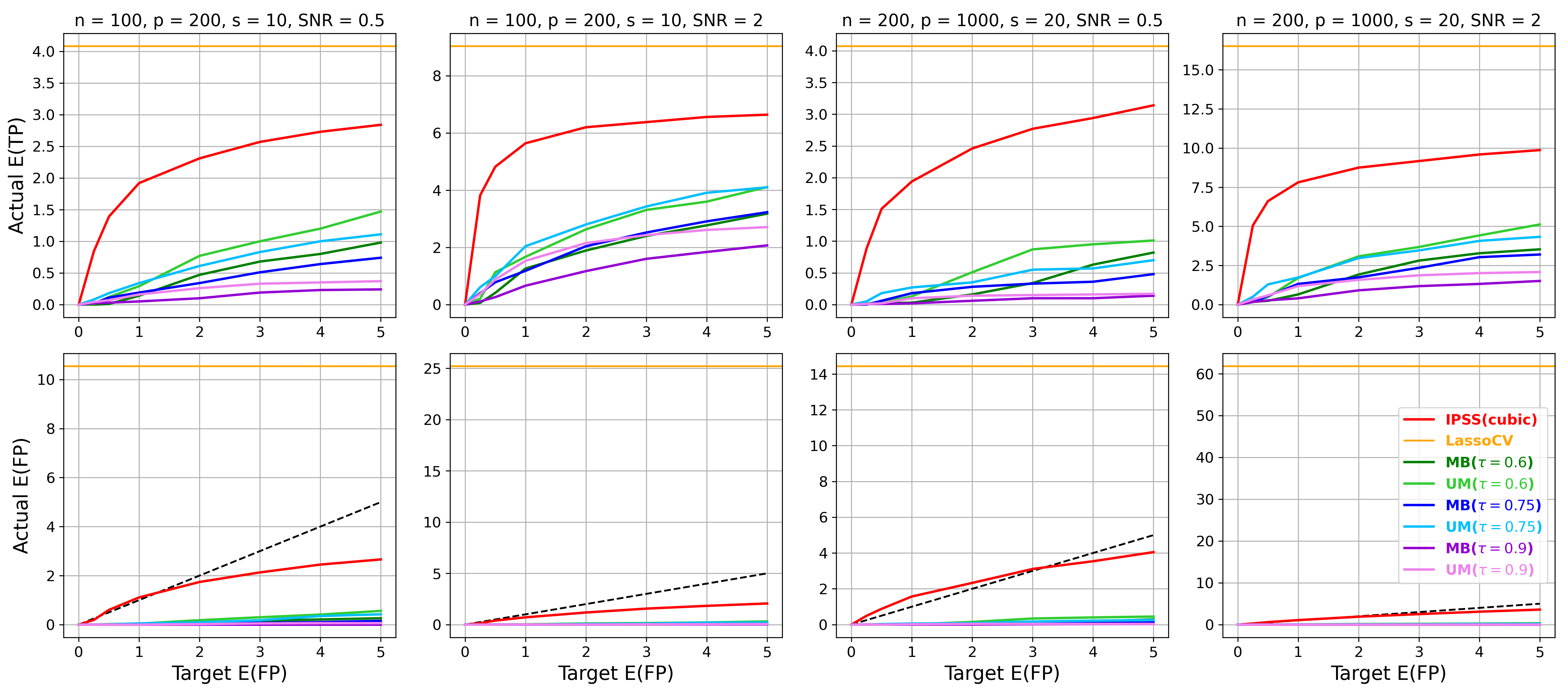
Figure S2. Linear regression with normal residuals and factor model design.

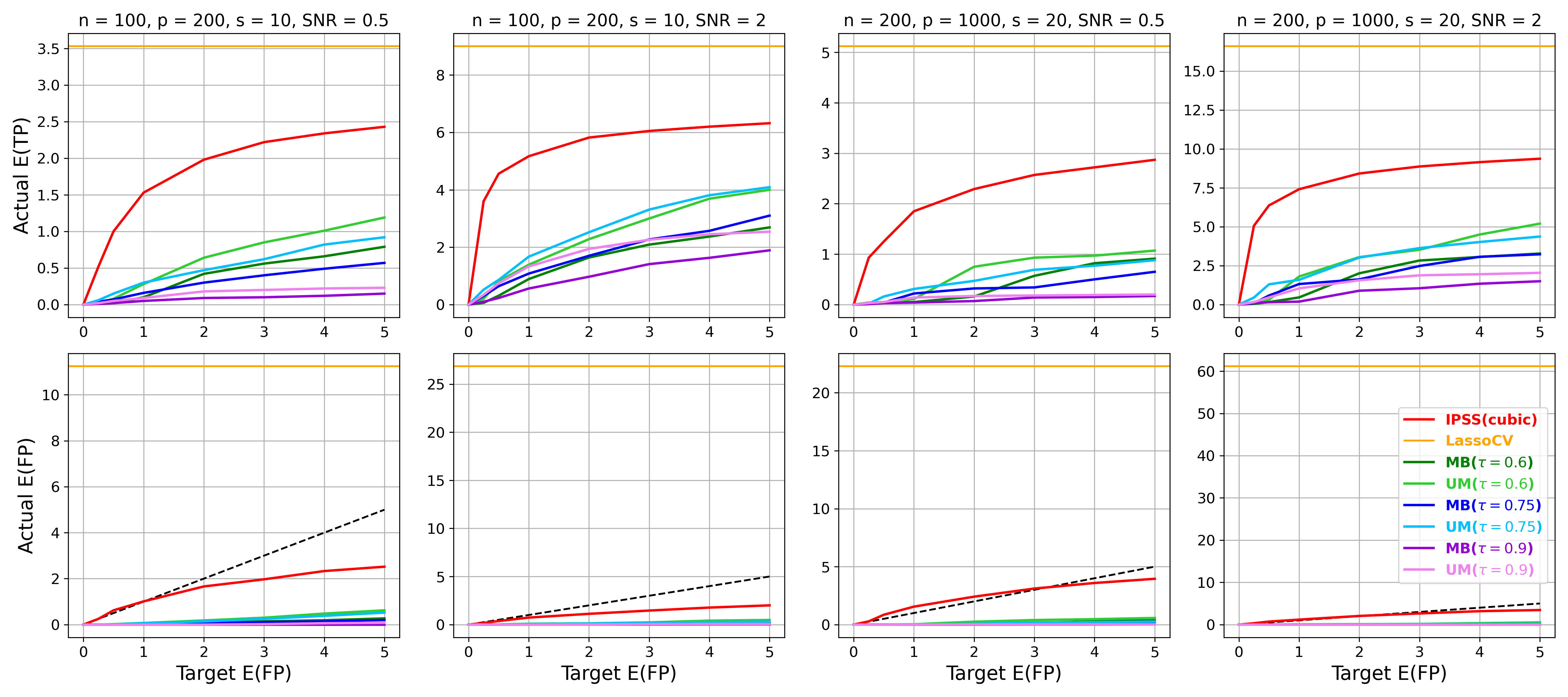
Figure S3. Linear regression with normal residuals and Toeplitz design ($\rho=0.5$).

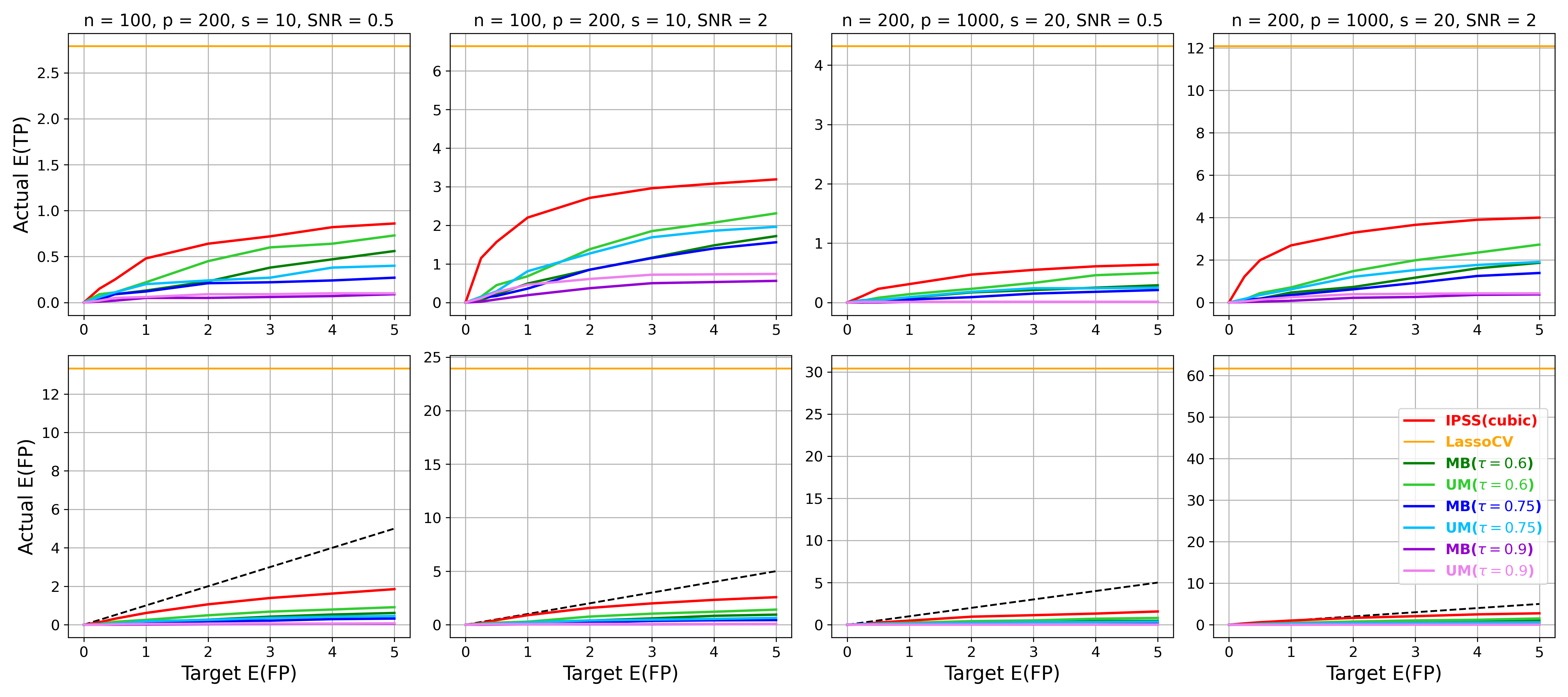
Figure S4. Linear regression with normal residuals and Toeplitz design ($\rho=0.9$).

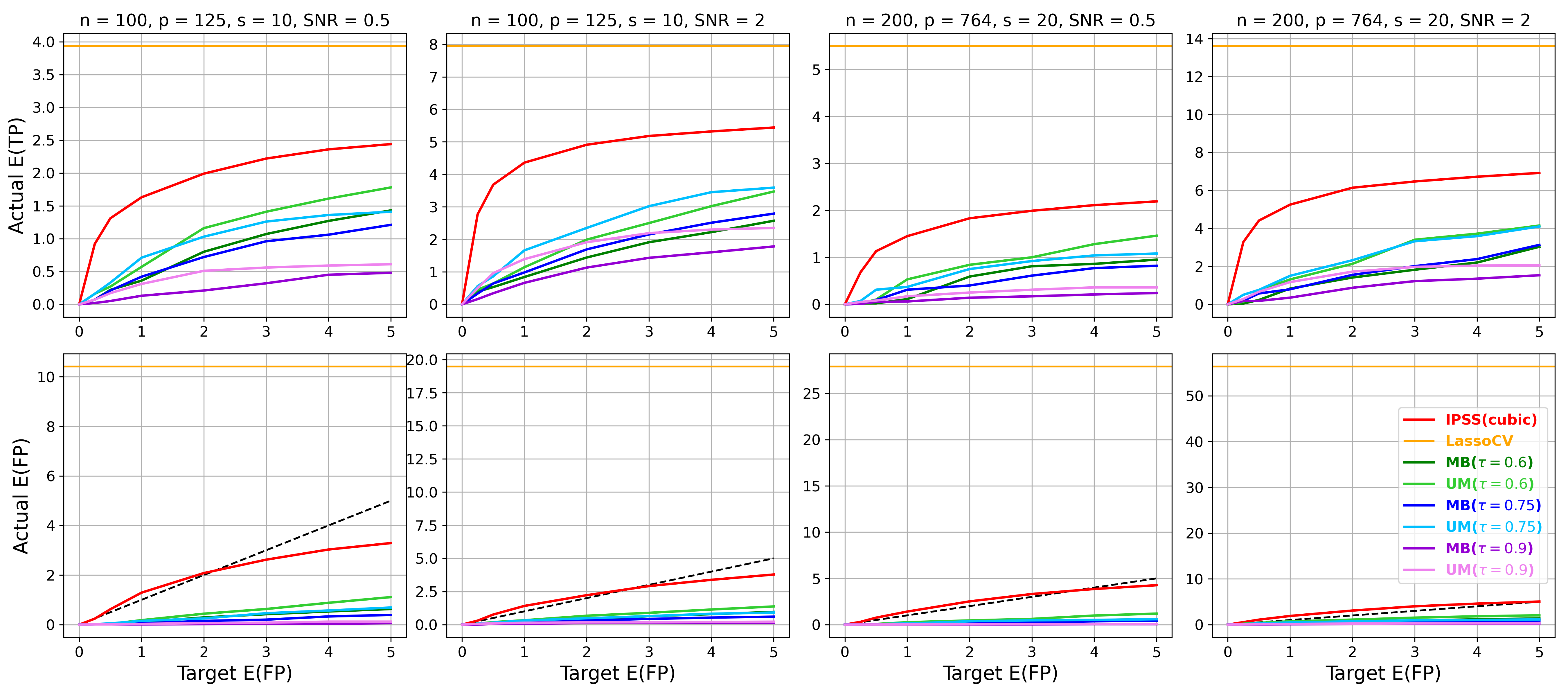
Figure S5. Linear regression with normal residuals and prostate cancer design.

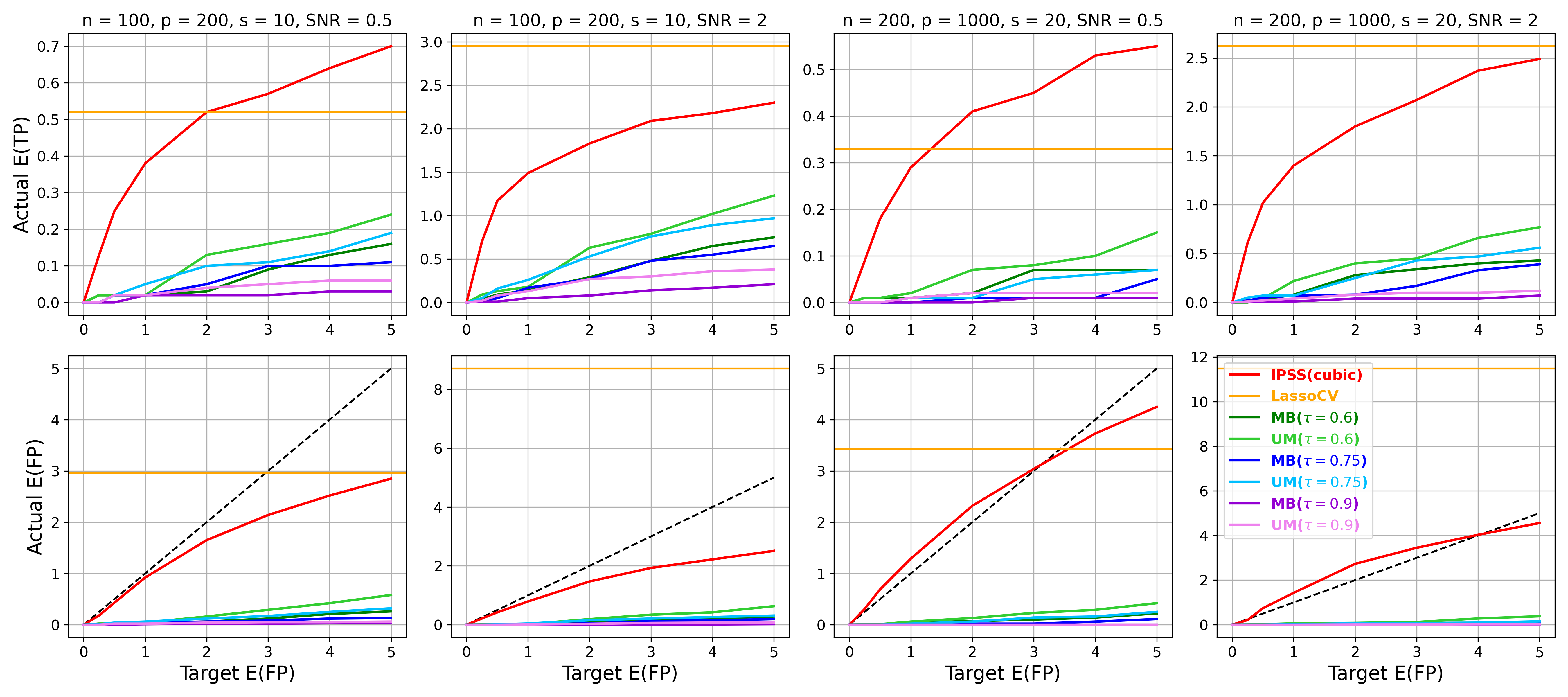
Figure S6. Linear regression with $t$ residuals and factor model design.

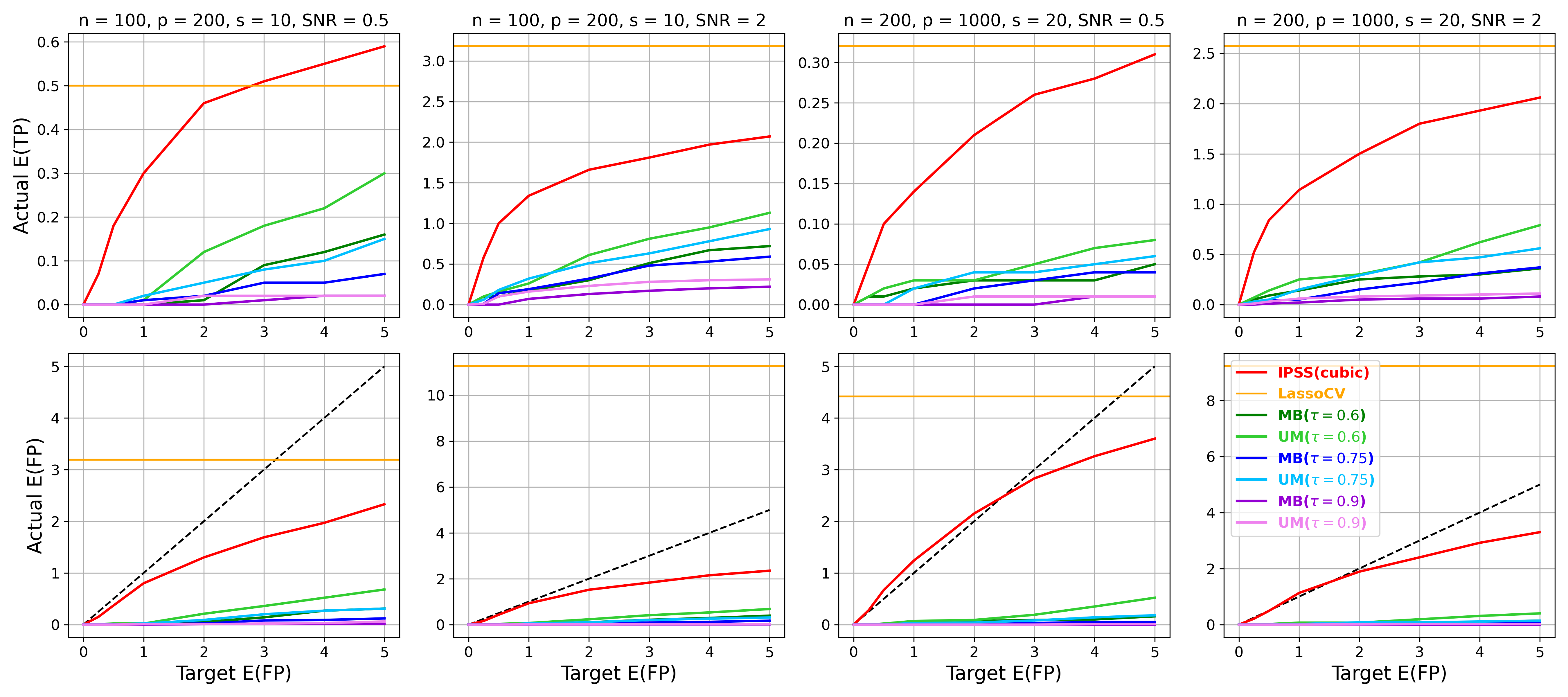
Figure S7. Linear regression with $t$ residuals and Toeplitz design ($\rho=0.5$).

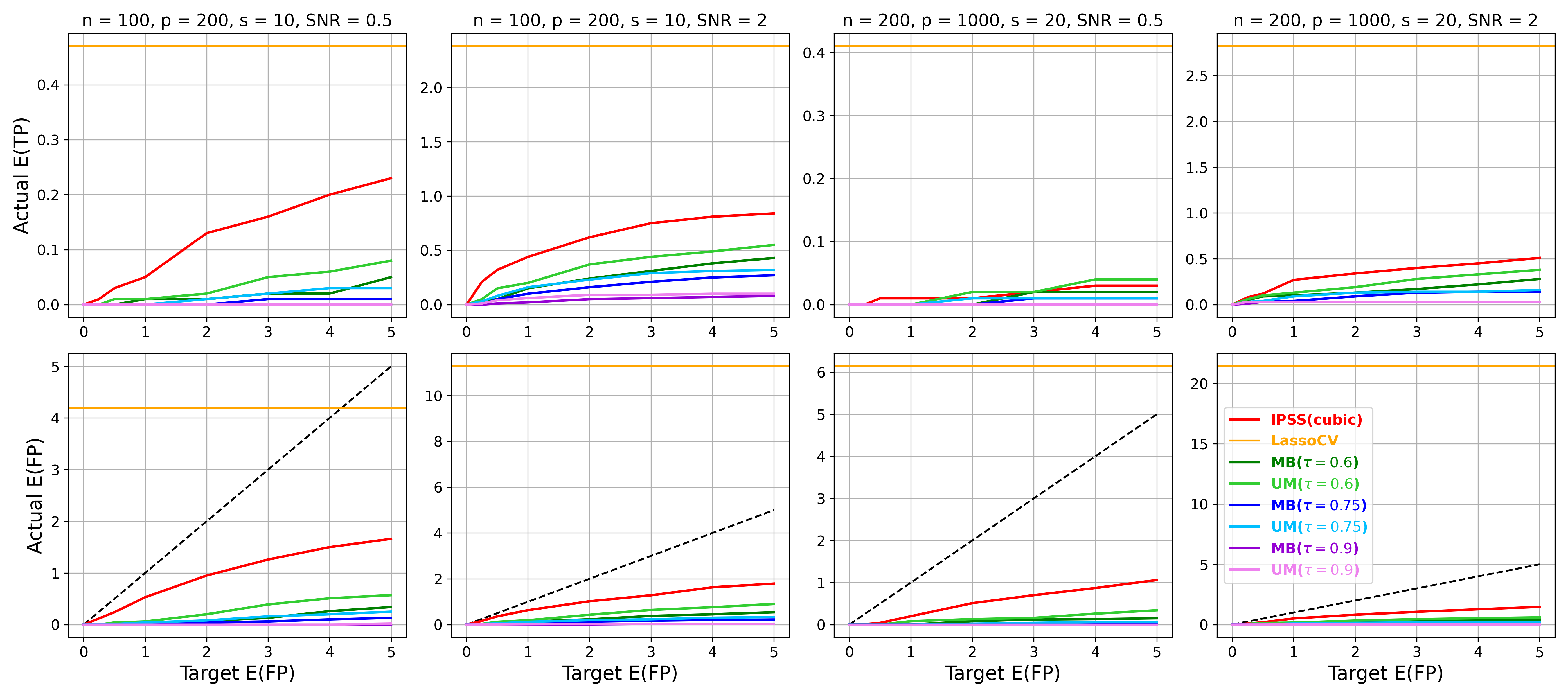
Figure S8. Linear regression with $t$ residuals and Toeplitz design ($\rho=0.9$).

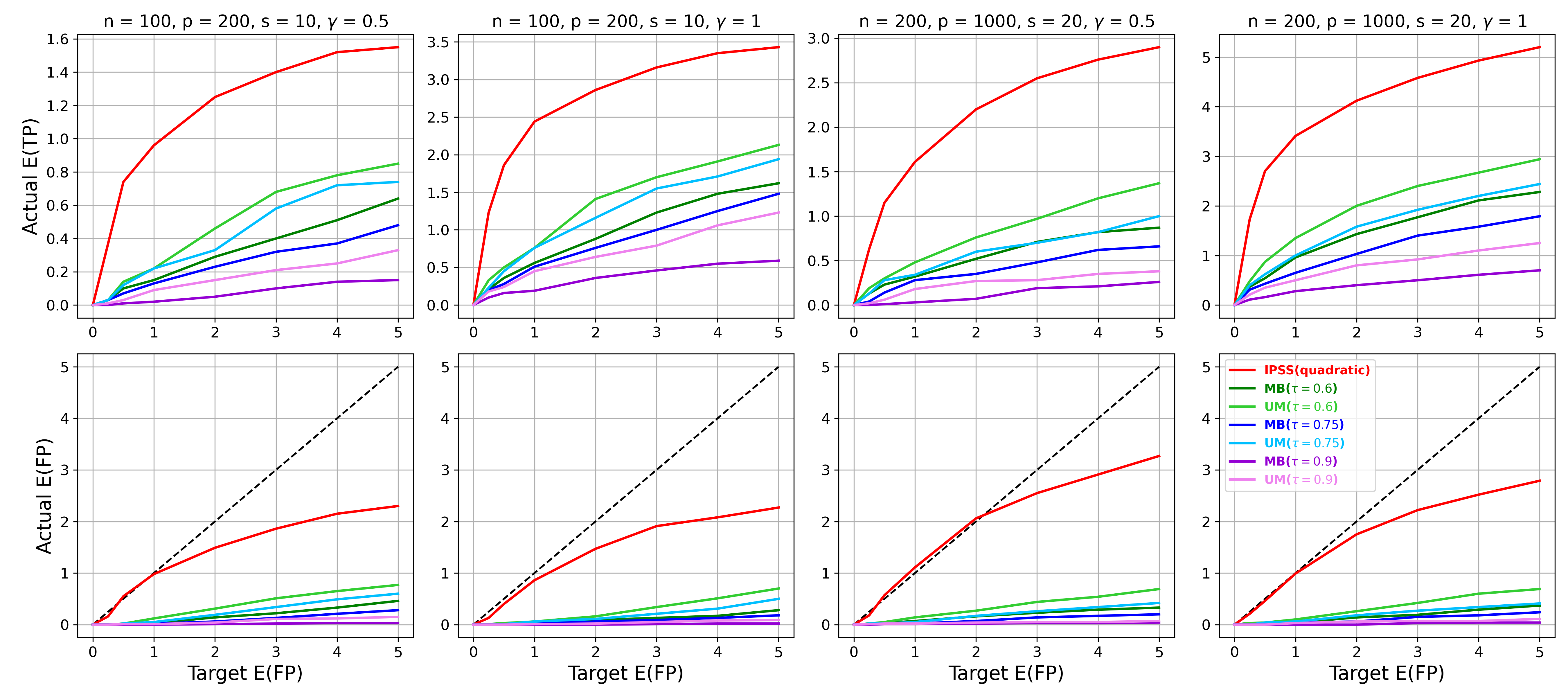
Figure S9. Logistic regression with factor model design.

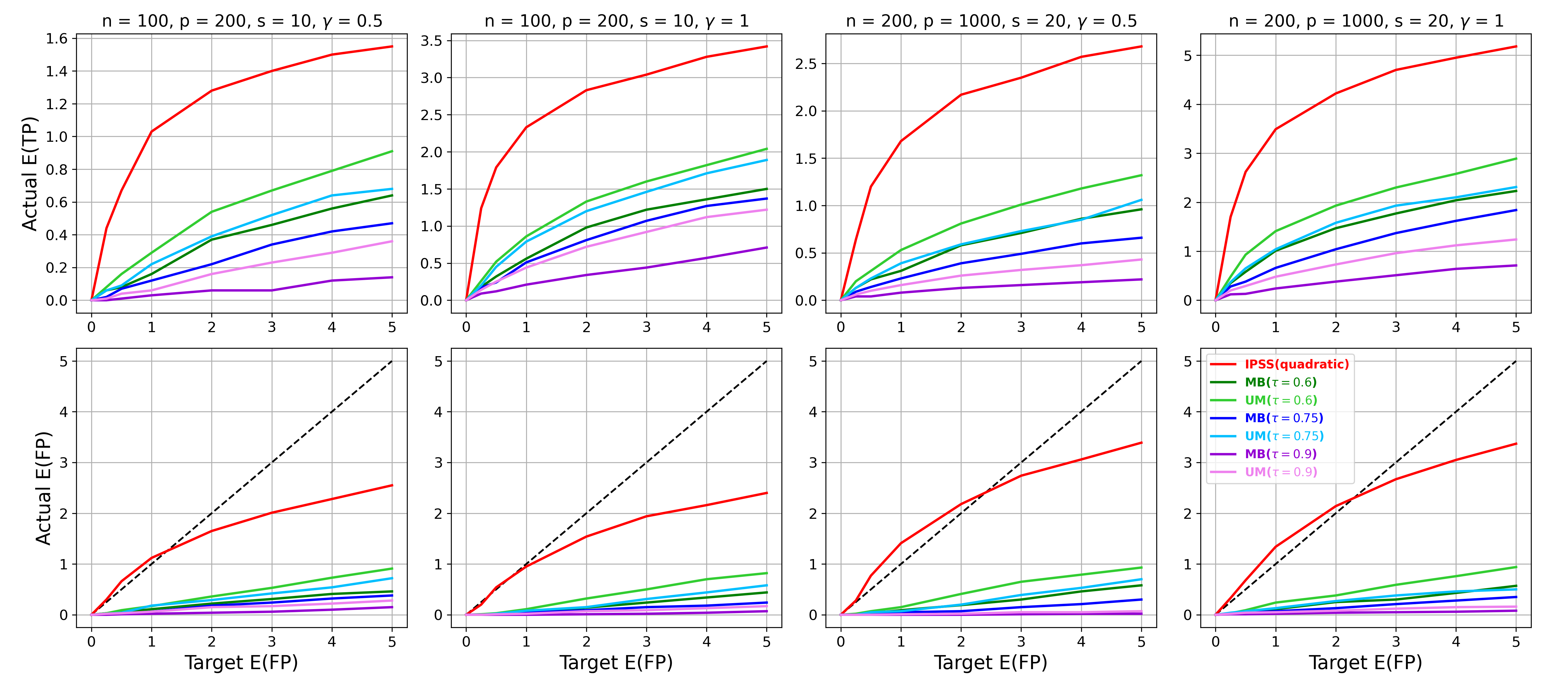
Figure S10. Logistic regression with Toeplitz design ($\rho=0.5$).

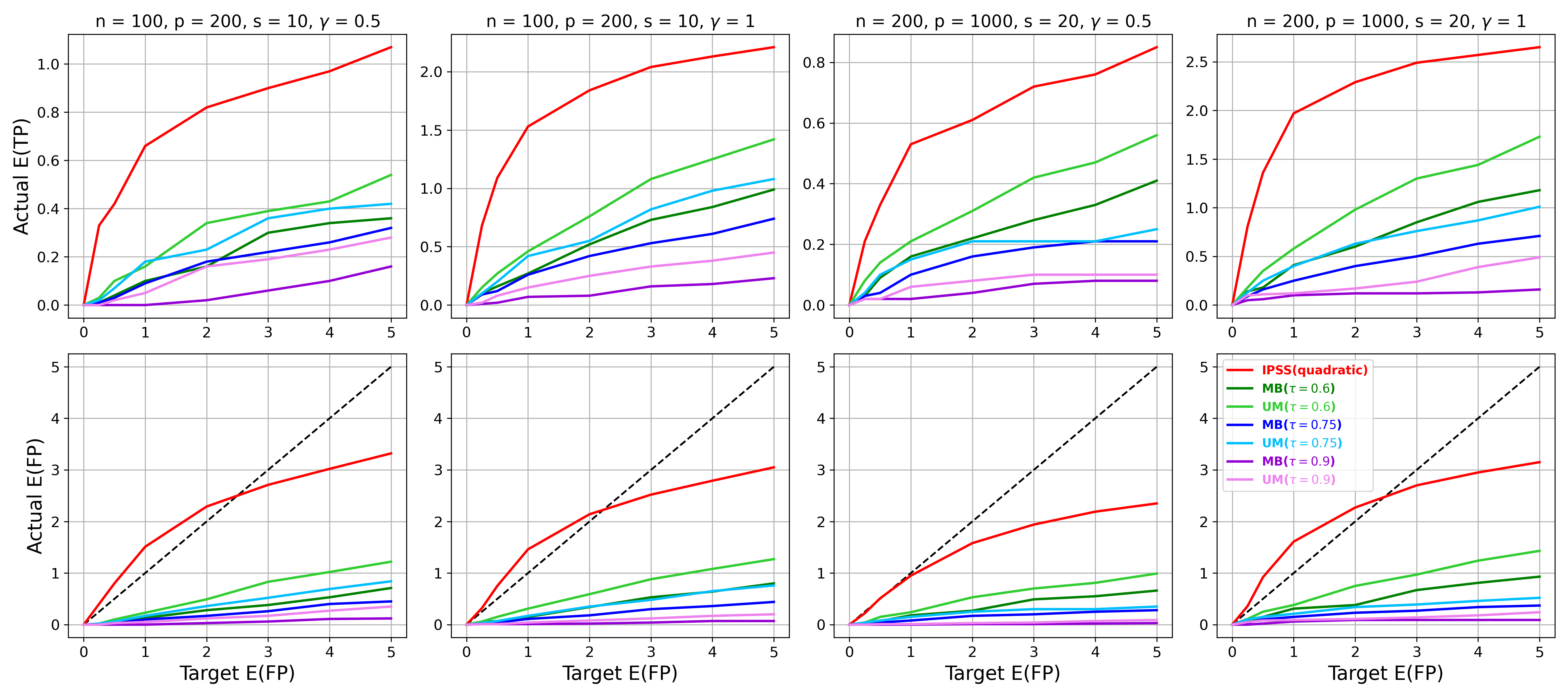
Figure S11. Logistic regression with Toeplitz design ($\rho=0.9$).

References

- Ahmed et al. (2011) I. Ahmed, A.-L. Hartikainen, M.-R. Järvelin, and S. Richardson. False discovery rate estimation for stability selection: application to genome-wide association studies. Statistical Applications in Genetics and Molecular Biology, 10(1), 2011.
- Alexander and Lange (2011) D. H. Alexander and K. Lange. Stability selection for genome-wide association. Genetic Epidemiology, 35(7):722–728, 2011.
- Alon et al. (1999) U. Alon, N. Barkai, D. A. Notterman, K. Gish, S. Ybarra, D. Mack, and A. J. Levine. Broad patterns of gene expression revealed by clustering analysis of tumor and normal colon tissues probed by oligonucleotide arrays. Proceedings of the National Academy of Sciences, 96(12):6745–6750, 1999.
- Anuraga et al. (2021) G. Anuraga, W.-C. Tang, N. N. Phan, H. D. K. Ta, Y.-H. Liu, Y.-F. Wu, K.-H. Lee, and C.-Y. Wang. Comprehensive analysis of prognostic and genetic signatures for general transcription factor III (GTF3) in clinical colorectal cancer patients using bioinformatics approaches. Current Issues in Molecular Biology, 43(1):2–20, 2021.
- Arentz et al. (2011) G. Arentz, T. Chataway, T. J. Price, Z. Izwan, G. Hardi, A. G. Cummins, and J. E. Hardingham. Desmin expression in colorectal cancer stroma correlates with advanced stage disease and marks angiogenic microvessels. Clinical Proteomics, 8(1):1–13, 2011.
- Chen et al. (2017) Y. Chen, Z. Zhang, J. Zheng, Y. Ma, and Y. Xue. Gene selection for tumor classification using neighborhood rough sets and entropy measures. Journal of Biomedical Informatics, 67:59–68, 2017.
- D’Abronzo and Ghosh (2018) L. S. D’Abronzo and P. M. Ghosh. eIF4E phosphorylation in prostate cancer. Neoplasia, 20(6):563–573, 2018.
- Friedman et al. (2008) J. Friedman, T. Hastie, and R. Tibshirani. Sparse inverse covariance estimation with the graphical lasso. Biostatistics, 9(3):432–441, 2008.
- Grossi et al. (2015) V. Grossi, G. Lucarelli, G. Forte, A. Peserico, A. Matrone, A. Germani, M. Rutigliano, A. Stella, R. Bagnulo, D. Loconte, et al. Loss of STK11 expression is an early event in prostate carcinogenesis and predicts therapeutic response to targeted therapy against MAPK/p38. Autophagy, 11(11):2102–2113, 2015.
- Haury et al. (2012) A.-C. Haury, F. Mordelet, P. Vera-Licona, and J.-P. Vert. TIGRESS: trustful inference of gene regulation using stability selection. BMC Systems Biology, 6(1):1–17, 2012.
- Hofner et al. (2015) B. Hofner, L. Boccuto, and M. Göker. Controlling false discoveries in high-dimensional situations: boosting with stability selection. BMC Bioinformatics, 16:1–17, 2015.
- Huang et al. (2018) J. Huang, A. Duran, M. Reina-Campos, T. Valencia, E. A. Castilla, T. D. Müller, M. H. Tschöp, J. Moscat, and M. T. Diaz-Meco. Adipocyte p62/SQSTM1 suppresses tumorigenesis through opposite regulations of metabolism in adipose tissue and tumor. Cancer Cell, 33(4):770–784, 2018.
- Jamaspishvili et al. (2018) T. Jamaspishvili, D. M. Berman, A. E. Ross, H. I. Scher, A. M. De Marzo, J. A. Squire, and T. L. Lotan. Clinical implications of PTEN loss in prostate cancer. Nature Reviews Urology, 15(4):222–234, 2018.
- Lee et al. (2006) S.-I. Lee, H. Lee, P. Abbeel, and A. Y. Ng. Efficient -regularized logistic regression. In Proceedings of the 21st National Conference on Artificial Intelligence (AAAI), volume 6, pages 401–408, 2006.
- Leng et al. (2006) C. Leng, Y. Lin, and G. Wahba. A note on the lasso and related procedures in model selection. Statistica Sinica, pages 1273–1284, 2006.
- Levy et al. (2002) A. Levy, R. Gal, R. Granoth, Z. Dreznik, M. Fridkin, and I. Gozes. In vitro and in vivo treatment of colon cancer by VIP antagonists. Regulatory Peptides, 109(1-3):127–133, 2002.
- Li and Zhang (2017) J.-L. Li and C.-X. Zhang. Ensembling variable selectors by stability selection for the Cox model. In 2017 International Conference on Machine Learning and Cybernetics (ICMLC), volume 1, pages 35–41. IEEE, 2017.
- Li et al. (2013) S. Li, L. Hsu, J. Peng, and P. Wang. Bootstrap inference for network construction with an application to a breast cancer microarray study. The Annals of Applied Statistics, 7(1):391, 2013.
- Maddu et al. (2022) S. Maddu, B. L. Cheeseman, I. F. Sbalzarini, and C. L. Müller. Stability selection enables robust learning of differential equations from limited noisy data. Proceedings of the Royal Society A, 478(2262):20210916, 2022.
- Mairal and Yu (2012) J. Mairal and B. Yu. Complexity analysis of the lasso regularization path. arXiv preprint arXiv:1205.0079, 2012.
- Meinshausen and Bühlmann (2010) N. Meinshausen and P. Bühlmann. Stability selection. Journal of the Royal Statistical Society Series B: Statistical Methodology, 72(4):417–473, 2010.
- Nomiri et al. (2022) S. Nomiri, R. Hoshyar, E. Chamani, Z. Rezaei, F. Salmani, P. Larki, T. Tavakoli, N. J. Tabrizi, A. Derakhshani, M. Santarpia, et al. Prediction and validation of GUCA2B as the hub-gene in colorectal cancer based on co-expression network analysis: In-silico and in-vivo study. Biomedicine & Pharmacotherapy, 147:112691, 2022.
- Qiu et al. (2007) T. Qiu, W. E. Grizzle, D. K. Oelschlager, X. Shen, and X. Cao. Control of prostate cell growth: BMP antagonizes androgen mitogenic activity with incorporation of MAPK signals in Smad1. The EMBO Journal, 26(2):346–357, 2007.
- Rice et al. (2019) M. A. Rice, E.-C. Hsu, M. Aslan, A. Ghoochani, A. Su, and T. Stoyanova. Loss of Notch1 activity inhibits prostate cancer growth and metastasis and sensitizes prostate cancer cells to antiandrogen therapies. Molecular Cancer Therapeutics, 18(7):1230–1242, 2019.
- Rodríguez-Berriguete et al. (2012) G. Rodríguez-Berriguete, B. Fraile, P. Martínez-Onsurbe, G. Olmedilla, R. Paniagua, and M. Royuela. MAP kinases and prostate cancer. Journal of Signal Transduction, 2012, 2012.
- Shah and Samworth (2013) R. D. Shah and R. J. Samworth. Variable selection with error control: another look at stability selection. Journal of the Royal Statistical Society Series B: Statistical Methodology, 75(1):55–80, 2013.
- Shi et al. (2007) X.-B. Shi, L. Xue, J. Yang, A.-H. Ma, J. Zhao, M. Xu, C. G. Tepper, C. P. Evans, H.-J. Kung, and R. W. deVere White. An androgen-regulated miRNA suppresses Bak1 expression and induces androgen-independent growth of prostate cancer cells. Proceedings of the National Academy of Sciences, 104(50):19983–19988, 2007.
- Shu et al. (2024) J. Shu, K. Xia, H. Luo, and Y. Wang. DARS-AS1: A Vital Oncogenic LncRNA Regulator with Potential for Cancer Prognosis and Therapy. International Journal of Medical Sciences, 21(3):571, 2024.
- Sun et al. (2011) L. Sun, H. Hu, L. Peng, Z. Zhou, X. Zhao, J. Pan, L. Sun, Z. Yang, and Y. Ran. P-cadherin promotes liver metastasis and is associated with poor prognosis in colon cancer. The American Journal of Pathology, 179(1):380–390, 2011.
- Sutton et al. (2019) M. N. Sutton, Z. Lu, Y.-C. Li, Y. Zhou, T. Huang, A. S. Reger, A. M. Hurwitz, T. Palzkill, C. Logsdon, X. Liang, et al. DIRAS3 (ARHI) blocks RAS/MAPK signaling by binding directly to RAS and disrupting RAS clusters. Cell Reports, 29(11):3448–3459, 2019.
- Tanaka et al. (2003) Y. Tanaka, M. V. Gavrielides, Y. Mitsuuchi, T. Fujii, and M. G. Kazanietz. Protein kinase C promotes apoptosis in LNCaP prostate cancer cells through activation of p38 MAPK and inhibition of the Akt survival pathway. Journal of Biological Chemistry, 278(36):33753–33762, 2003.
- Tibshirani (1996) R. Tibshirani. Regression shrinkage and selection via the lasso. Journal of the Royal Statistical Society Series B: Statistical Methodology, 58(1):267–288, 1996.
- Ushigome et al. (2005) M. Ushigome, T. Ubagai, H. Fukuda, N. Tsuchiya, T. Sugimura, J. Takatsuka, and H. Nakagama. Up-regulation of hnRNP A1 gene in sporadic human colorectal cancers. International Journal of Oncology, 26(3):635–640, 2005.
- Vasaikar et al. (2018) S. V. Vasaikar, P. Straub, J. Wang, and B. Zhang. LinkedOmics: analyzing multi-omics data within and across 32 cancer types. Nucleic Acids Research, 46(D1):D956–D963, 2018.
- Wang et al. (2020) F. Wang, S. Mukherjee, S. Richardson, and S. M. Hill. High-dimensional regression in practice: an empirical study of finite-sample prediction, variable selection and ranking. Statistics and Computing, 30:697–719, 2020.
- Wang et al. (2010) S.-L. Wang, X. Li, S. Zhang, J. Gui, and D.-S. Huang. Tumor classification by combining PNN classifier ensemble with neighborhood rough set based gene reduction. Computers in Biology and Medicine, 40(2):179–189, 2010.
- Werner (2023) T. Werner. Loss-guided stability selection. Advances in Data Analysis and Classification, pages 1–26, 2023.
- Zhang et al. (2020) J. Zhang, S. Li, L. Zhang, J. Xu, M. Song, T. Shao, Z. Huang, and Y. Li. RBP EIF2S2 promotes tumorigenesis and progression by regulating MYC-mediated inhibition via FHIT-related enhancers. Molecular Therapy, 28(4):1105–1118, 2020.
- Zhou et al. (2013) J. Zhou, J. Sun, Y. Liu, J. Hu, and J. Ye. Patient risk prediction model via top-k stability selection. In Proceedings of the 2013 SIAM International Conference on Data Mining, pages 55–63. SIAM, 2013.
- Zou (2006) H. Zou. The adaptive lasso and its oracle properties. Journal of the American Statistical Association, 101(476):1418–1429, 2006.
- Zou and Hastie (2005) H. Zou and T. Hastie. Regularization and variable selection via the elastic net. Journal of the Royal Statistical Society Series B: Statistical Methodology, 67(2):301–320, 2005.