iA^∗: Imperative Learning-based A^∗ Search for Pathfinding

Abstract

The pathfinding problem, which aims to identify a collision-free path between two points, is crucial for many applications, such as robot navigation and autonomous driving. Classic methods, such as A^∗ search, perform well on small-scale maps but face difficulties scaling up. Conversely, data-driven approaches can improve pathfinding efficiency but require extensive data labeling and lack theoretical guarantees, making it challenging for practical applications. To combine the strengths of the two methods, we utilize the imperative learning (IL) strategy and propose a novel self-supervised pathfinding framework, termed imperative learning-based A^∗ (iA^∗). Specifically, iA^∗ is a bilevel optimization process where the lower-level optimization is dedicated to finding the optimal path by a differentiable A^∗ search module, and the upper-level optimization narrows down the search space to improve efficiency via setting suitable initial values from a data-driven model. Besides, the model within the upper-level optimization is a fully convolutional network, trained by the calculated loss in the lower-level optimization. Thus, the framework avoids extensive data labeling and can be applied in diverse environments. Our comprehensive experiments demonstrate that iA^∗ surpasses both classical and data-driven methods in pathfinding efficiency and shows superior robustness among different tasks, validated with public datasets and simulation environments.

I INTRODUCTION

Pathfinding is one of the most basic research topics in robot navigation, determining a route from a starting position to a destination given an environment [1]. It is critical for robots to navigate in environments with obstacles and may also optimize specific criteria such as the shortest distance, minimal energy use, or maximum safety [2].

The search-based method, such as Dijkstra’s algorithm [3], is one of the most popular branches in the field of pathfinding. It can always find the shortest path, if one exists, by incrementally searching all nodes in the given map. To avoid searching all nodes, heuristic strategies are introduced to the search-based pathfinding by providing a potential search direction in the given map, such as A^∗[4] search and D^∗ search [5]. Compared with other pathfinding methods, such as sampling-based pathfinding [6], the search-based pathfinding can guarantee finding the shortest path. Thus, the search-based pathfinding has received great popularity in real applications, such as autonomous vehicle navigation [7] and video game [8]. However, the search-based pathfinding is time-consuming due to the exponential time complexity growth incurred by the increasing size of the map [9], which is unacceptable in robot navigation applications that need immediate responses to the dynamic environmental changes.

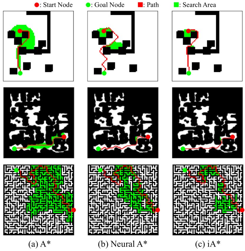
Figure 1: The difference between selected search-based pathfinding methods. (a), (b), and (c) display the pathfinding results by using A^∗, Neural A^∗, and iA^∗ (ours), where the red and green circles represent the start node and goal node while the red pixels and green pixels represent the generated path and search area.

Recently, with the advancement of neural networks, some researchers [10, 11] have adopted data-driven strategies to improve the efficiency of search-based pathfinding. They use the optimal paths to train their integrated networks, adding some constraints to the given map. With these constraints, these methods can reduce the search space and still efficiently get the near-optimal paths with an acceptable slight increase in path length. However, the limitations of the data-driven methods are apparent. The natures of these data-driven methods are still black-box models with poor interpretability, so they lack guarantees when applied to practical robotic tasks. Additionally, these methods need extensive, well-labeled data, demanding significant pre-processing time from researchers, and often struggle with overfitting, limiting their effectiveness to scenarios similar to the training data.

To solve the mentioned problems in data-driven pathfinding and improve the pathfinding efficiency, we introduce the imperative learning (IL) strategy into search-based pathfinding and propose the imperative A^∗ (iA^∗). IL is an emerging learning framework leveraging the advantages of both data-driven and classical methods, which has been applied to local planning [12], SLAM [13], and feature correspondence [14]. The core of iA^∗ is a bilevel optimization process [15], where the upper-level optimization is to train a neural network for reducing the search space, and the lower-level optimization is an interpretable A^∗ for finding the optimal path given the search space. Since the lower-level A* search can be optimized without providing any labels, the entire framework of iA^∗ can be trained in a self-supervised manner. In this way, we avoid preparing the well-labeled training data and increase the interpretability. The experimental results demonstrate that iA^∗ can find the near-optimal solution and significantly improve the search efficiency.

Our core contributions are shown as follows:

• To improve search efficiency and add interpretability, we propose an IL-based A^∗ search framework (iA^∗) that includes a bilevel optimization process to achieve the near-optimal solution with high efficiency. To solve the challenge of data labeling, the framework adopts a self-supervised manner to train the integrated encoder.

• To achieve the trade-off between path length and search efficiency, we modify the existing differentiable A^∗ (dA^∗) search algorithm in lower-level optimization and design a target function as a combination of path length and search area in upper-level optimization.

• Experimental results demonstrate that the proposed iA^∗ outperforms both classical and learning-based pathfinding methods, which averagely reduces 67.2% search area and saves 58.3% runtime across diverse maps.

To promote the development of robotic pathfinding, both the source codes of dA^∗ and iA^∗ will be released and integrated into our open-source PyPose library [16].

II Related Works

II-A Classical Pathfinding

The pathfinding problem, getting the collision-free path from the start node to the goal node with a given map, has developed for many years. In the beginning, the classical works solve the pathfinding problem by graph-search approach [17] that iteratively searches the nodes from the start node to the goal node, such as Breadth First Search. After that, some algorithms, such as Greedy BFS [18], A^∗ [4], and D^∗ [19], introduce the heuristic information and provide a search direction to improve the pathfinding efficiency. These heuristic search-based algorithms can find the optimal path when their suitable heuristic functions are admissible. However, the search-based pathfinding methods face the problem of low search efficiency with the increasing size of maps due to their exponential time complexity growth.

Unlike search-based pathfinding methods, sampling-based methods sample nodes in the given map and connect nodes to find their solution. As the number of sampling points increases, the solution is closer to the optimal path. Typically, they stop their sampling to improve their search efficiency when finding a near-optimal path acceptable in the given task. The sampling-based methods can alleviate the computation growth by increasing the size of maps. By using a tree structure to store nodes and establish connections between the sampled points, some methods have outstanding performance, such as RRT [20] and its derivatives [21, 22, 23, 24]. Besides, some sampling-based pathfinding methods [25, 26, 27] utilize the probabilistic road map to get solutions. However, these sampling-based methods can only get the near-optimal solution and may fail to find a solution in complex environments with high obstacle density.

II-B Learning-based Pathfinding

Recently, with the development of deep learning technology, plenty of learning-based pathfinding methods have appeared. Some of them utilize the networks to extract environmental information and provide guidance for improving search efficiency. SAIL [28] aims to find a suitable heuristic function that could observe and process the whole map instead of the local map during pathfinding. Besides, [29] and TransPath [11] integrate the U-net-based model [30] and Transformer-based model [31] to learn their heuristic functions, respectively. Some methods [32, 10] utilize their well-trained network to encode the original map to generate a guidance map. Then, the guidance map allows them to decrease their search area and improve their search efficiency. MPNet[33] uses two networks, Encoder net (Enet) and Planning net (Pnet), for the pathfinding task, where Enet handles the environment information, and Pnet can provide the next state of the robot under the current situation.

Some researchers use reinforcement learning (RL) [34] to solve the pathfinding task. They aim to find the end-to-end solution for the pathfinding task without any policies. They formulate the pathfinding problem as the Markov decision processes that the next state in the path depends on the current state and surroundings. [35] demonstrates that it is possible to solve the pathfinding problem in grid maps using the RL-based method. [36] combines the path graph with Q-learning, efficiently finding the optimal path. However, these learning-based methods face problems of lacking interpretability and extensive data labeling.

II-C Imperative Learning

Imperative learning (IL) is an emerging self-supervised learning framework based on bilevel optimization, where upper-level optimization is a data-driven model and lower-level optimization is an interpretable algorithm. The results from lower-level optimization guide the training of the data-driven model within upper-level optimization, achieving a self-supervised manner. For example, iPlanner [12] utilizes a data-driven model to guide the B-spline interpolation algorithm, generating safe and smooth trajectories with depth images. iSLAM [13] adopts the IL framework to integrate the front-end and back-end of visual odometry. It utilizes a network to guide the pose estimation to generate the poses aligned with geometrical reality. Moreover, iMatching [14] utilizes a network to guide the feature matching process that allows the bundle adjustment module to generate the optimal translation matrix. These works demonstrate the efficiency of IL in robot navigation tasks. Thus, we propose the iA^∗ search framework. To the best of our knowledge, iA^∗ is the first method using the IL strategy to solve pathfinding problems.

III Preliminaries

Before discussing the proposed iA^∗ framework, it is necessary to explain the details of the classical A^∗ search algorithm. The A^∗ search algorithm is a graph traversal technique that aims to identify the shortest path from a start node to a goal node under a given Graph $G$. Classical A^∗ search works by incrementally searching the nodes with the prioritized heuristic information. Specifically, open-list $\mathcal{O}$ and closed-list $\mathcal{C}$ are set to store the nodes that are waiting to be visited and the nodes that have already been visited, respectively. Mathematically, in each step of node selection, A^∗ always selects the node from $\mathcal{O}$ with minimum cost calculated by the cost function $c(n)$, shown as:

$$c(n)=s(n)+h(n),$$ (1)

where $s(n)$ is the accumulated path length from start node to node $n$, and $h(n)$ is the estimated heuristic distance from node $n$ to the goal node. The heuristic distance can be calculated using different strategies such as Manhattan, Euclidean, and Chebyshev distances. Theoretically, it is guaranteed to have the least-cost path without processing any node more than once if the heuristic $h(n)$ is admissible and monotone (consistent), i.e., $\forall m\in G,h(n)\leq d(m,n)+h(m)$, where $d(m,n)$ is the path cost from node $m$ to node $n$. The pseudo-code of A^∗ search is shown in Algorithm 1. Our work is based on the classical A^∗ search algorithm and uses learning technology to improve efficiency.

IV Methodology

IV-A Framework

To leverage the advantages of both learning-based and search-based pathfinding methods, imperative A^∗ (iA^∗) adopts the imperative-learning (IL), including learning-based upper-level optimization and classical A^∗ based lower-level optimization. The framework of iA^∗ is depicted in Fig. 2, which takes a planning instance as input, a three-layer tensor containing the information of the obstacles, start, and goal positions, and outputs the near-optimal path (red) and search area (green). Within the framework, the instance encoder module is the crucial part of upper-level optimization; the A^∗ search module represents the lower-level optimization; the memory module contains the intermediate information and establishes a bridge between these optimizations. Upper-level optimization aims to narrow down the search space, while lower-level optimization is dedicated to identifying the optimal path under specific conditions. Specifically, this iA^∗ framework can be formulated as:

$$\min_{\theta}\quad U\left(f(\theta,\bm{x}),\mu^{*})\right),$$ (2a)

s.t. $$\mu^{*}=\arg\min_{\mu}L(f,\mu,M),$$ (2b)

where $\bm{x}$ denotes the input instance, including the map, start node, and goal node, $\theta$ represents the neuron-like learnable parameters, and $f(\theta,\bm{x})$ is the encoding process of instance encoder $f$, and $\mu$ is the set of paths in the solution space. Eq. (2a) represents the upper-level optimization to obtain the optimal parameters of the instance encoder, aiming to improve the search efficiency, while Eq. (2b) is the lower-level optimization to get the optimal path with minimum $s$ value under the given map $M$ and the instance encoder $f$ The lower-level optimization is directly solvable because the A^∗ search algorithm always has a closed-form solution.

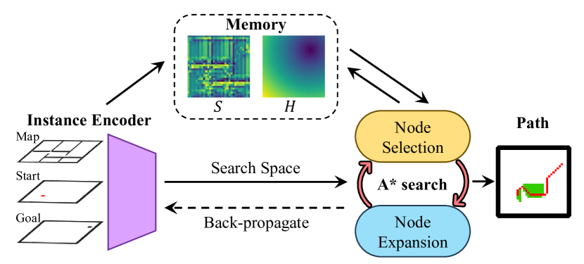
Figure 2: The framework of iA^∗. The input is a three-layer tensor containing map information, start node, and goal node, and the output is the path with the search area. It mainly has three parts: the Instance Encoder, the Memory Storage, and the A^∗ search.

IV-B Lower-level Optimization

The lower-level optimization is the $A^{*}$ search algorithm, finding the optimal path given the input instance. In the designed framework, the lower-level optimization receives the encoding results from upper-level optimization and back-propagates the loss to train the instance encoder. However, the classical A^∗ uses the graph structure, discretely storing nodes in the map with parameters. The discrete representation presents challenges in establishing connections with upper-level optimization and training efficiency. Thus, we change the $A^{*}$ search algorithm to a differentiable fashion with a matrix representation, similar to [10].

Firstly, all the variables and parameters in Algorithm 1 are transformed into matrix form. Specifically, we use the binary matrices with the same size as the given map, $O$, $C$, and $N$, representing the nodes contained in $\mathcal{O}$, $\mathcal{C}$ and $\mathcal{N}$, respectively. The start node $n_{s}$, the goal node $n_{g}$, and the selected node $n^{\prime}$ are also transformed into one-hot indicator matrices $N_{s}$, $N_{g}$, and $N^{\prime}$. The one-hot indicator matrix only has one element whose value is 1, and the other elements are 0. The values $s,h$ of each node are also stored in matrices $S$ and $H$. Secondly, in Algorithm 1, the discrete operations must be transformed into matrix operations, including the node selection part (Line 3), node expansion part (Line 10), and value $s$ update (Line 13 and Line 19). The details of the transformation are explained in the following paragraphs.

Node Selection: This step selects the node $n^{\prime}$ with minimum $C(n)$ in the $\mathcal{O}$. To achieve the same function in a matrix representation, node selection is formulated as follows:

$$N^{\prime}=\mathcal{L}_{\max}{\left(\frac{\exp(-(S+H)/\tau)\odot O}{<\exp(-(S+H)/\tau),O>}\right)},$$ (3)

where $A\odot B$ is Hadamard product[37], $\tau$ is an empirically defined parameter, $\mathcal{L}_{max}(A)$ is the function to obtain the $argmax$ index matrix of A, and $O$ is the open-list matrix to ensure that the selected node is from the open-list.

Node Expansion: The node expansion part extracts the neighboring nodes of the selected node $n^{\prime}$. In the grid map, one node typically has eight neighboring nodes. This process is formulated as a convolution operation between $N^{\prime}$ and the fixed kernel $K=[[1,1,1]^{T},[1,0,1]^{T},[1,1,1]^{T}]$. Besides, the neighboring nodes should exclude the position of obstacles and nodes in the open-list $O$ and closed-list $C$. Then, we can get the matrix of neighboring nodes $N_{\text{nbr}}$, and the whole formulation is shown as follows:

$$N_{\text{nbr}}=(N^{\prime}*K)\odot X\odot(\mathbbm{1}-O)\odot(\mathbbm{1}-C),$$ (4)

where $A*B$ is the convolution operation between matrix $A$ and kernel $B$ and the matrix $X$ contains the obstacle configuration of the given map, setting the obstacle positions with 0 and the free positions with 1. The series of $\odot$ operations can be seen as several masks, excluding nodes from obstacles $X$, open-list $O$, and closed-list $C$.

Algorithm 1 A^∗ Search Algorithm

1:$m$: map; $n_{s}$: Start Node; $n_{g}$: Goal Node; $\mathcal{O}$: Open List; $\mathcal{C}$: Closed List; $\mathcal{N}$: Node Set;

2:$\mathcal{P}$: Shortest Path

3:$\mathcal{O}\leftarrow\{n_{s}\}$; $s(n_{s})\leftarrow 0;\forall n\in\mathcal{N}\backslash\{n_{s}\},s(n)\leftarrow\infty$;

4:$\text{Parent}{n_{s}}\leftarrow\emptyset$;

5:while  $\mathcal{O}\neq\{\}$ do

6:     $n^{\prime}\leftarrow\underset{n\in\mathcal{O}}{\arg\min}(s(n)+h(n))$;

7:     remove $n^{\prime}$ from $\mathcal{O}$;

8:     insert $n^{\prime}$ into $\mathcal{C}$;

9:     if $n^{\prime}=n_{g}$ then

10:         $\mathcal{P}\leftarrow\text{Backtrack}(\text{Parent},n_{g})$;

11:         return $\mathcal{P}$;

12:     end if

13:     extract $\mathcal{N}_{\text{nbr}}\leftarrow\text{NodeExpansion}(n^{\prime})$;

14:     for $n\in\mathcal{N}_{\text{nbr}}$ do

15:         if $n\in\mathcal{O}$ then

16:              if $s(n)>s(n^{\prime})+d(n^{\prime},n)$ then

17:                  $s(n)\leftarrow s(n^{\prime})+d(n^{\prime},n)$

18:                  $\text{Parent}(n)\leftarrow n^{\prime}$

19:              end if

20:         else

21:              insert $n$ into $\mathcal{O}$

22:              $s(n)\leftarrow g(n^{\prime})+d(n^{\prime},n)$;

23:              $\text{Parent}(n)\leftarrow n^{\prime}$

24:         end if

25:     end for

26:end while

Value $s$ Update: $s(n)$ represents the cost from the $n_{s}$ to the current node $n$. With the progress of searching, the $s$ value of each node is also updated synchronously. In matrix representation, this process is transformed into updating the $S$ matrix in each iteration, which is shown as follows,

$$S^{\prime}=<S,N^{\prime}>\odot N_{\text{nbr}}+N^{\prime}*K_{c},$$ (5a)

$$K_{c}=[[\sqrt{2},1,\sqrt{2}]^{T},[\sqrt{2},0,\sqrt{2}]^{T},[\sqrt{2},1,\sqrt{2}]^{T}],$$ (5b)

$$S=\min(S\odot N_{\text{nbr}},S^{\prime})+S\odot(\mathbbm{1}-N_{\text{nbr}}).$$ (5c)

where $K_{c}$ is a cost kernel calculated by the Euclidean Distance between the selected node $N^{\prime}$ and its neighboring nodes $N_{\text{nbr}}$, $S^{\prime}$ is the intermediate matrix of $s$ values of $N_{\text{nbr}}$ in the current step, and $S$ is the updated matrix of $s$ values.

IV-C Upper-level Optimization

The upper-level optimization aims to improve search efficiency by providing initial $s$ values for each node. In the classical A^∗ algorithm, the $s$ values of the unvisited nodes are set as infinity, resulting in all unvisited nodes having the same possibility of being selected, even though some of them will face dead ends. Because deep-learning technology has some advantages of extracting information and generating suitable encoding fashion, we expect the instance encoder within upper-level optimization can generate a suitable initial $s$ value for each node according to the given instance with obstacles, start, and goal positions. In this way, iA^∗ can avoid unnecessary searches and improve the pathfinding efficiency.

Instance Encoder: We expect the proposed framework to handle diverse environments with different sizes without changing the network structure. To this purpose, the instance encoder is designed as a fully convolutional network architecture [38] with three convolution layers because the convolution operation can use tensors with different sizes as their inputs, while other operations, such as matrix multiplication, need their inputs with a fixed size. This usage significantly avoids retraining the network in new environments and provides convenience in robot applications.

Network Training: To avoid the problem of data labeling, the training process adopts a self-supervised manner. The pathfinding results from the lower-level optimization directly guide the training of the instance encoder within the upper-level optimization. To be specific, only raw environmental maps are provided as training data. Then, the start and goal positions are randomly selected, and the integrated differentiable A^∗ algorithm tests whether there is a solution under the given conditions. If there is, the framework will automatically calculate loss according to the target function $U$ and use it to train the instance encoder.

Here, to achieve the trade-off between search efficiency and path length, we define the target function $U$ as the combination of the loss of search area $\mathcal{L}_{a}(\mu)$ and the loss of path length $\mathcal{L}_{l}(\mu)$. In this way, the proposed iA^∗ framework achieves a smaller search area while ensuring the path is still close to the optimal one. The area loss $\mathcal{L}_{a}$ is calculated as the sum of visited nodes, which can be formulated as:

$$\mathcal{L}_{a}(\mu)=\sum C_{\mu},$$ (6)

where $C_{\mu}$ contains all visited nodes when finding the path $\mu$. Besides, $\mathcal{L}_{l}(\mu)$ is the length of path $\mu$ generated from the A^∗ module, which is calculated by matrix product as follows:

$$\mathcal{L}_{l}(\mu)=\frac{\left<\mu*K_{c},\mu\right>}{2},$$ (7)

where $\mu$ is the path generated, and $K_{c}$ is the cost kernel defined in Eq. (5). Finally, the target function of the upper-level optimization is mathematically represented as:

$$U(\mu^{*}):=w_{a}\mathcal{L}_{a}(\mu^{*})+w_{l}\mathcal{L}_{l}(\mu^{*}),$$ (8)

where $\mathcal{L}_{a}(\mu^{*})$ and $\mathcal{L}_{l}(\mu^{*})$ are the search area and path length losses, given the path $\mu^{*}$, and $w_{a}$ and $w_{l}$ are the weights to adjust the ratio of the calculated losses. In this way, the proposed framework narrows the search area to improve search efficiency and still finds the near-optimal path.

V Experiments

In this section, we conduct experiments to assess the performance of iA^∗ on improving search efficiency, i.e., how much time the iA^∗ saves in the pathfinding problem. We select the latest data-driven pathfinding methods to make comparisons with iA^∗ and three widely-used datasets to provide pathfinding instances in diverse environments. Moreover, to test the performance of the iA^∗ algorithm in robot navigation tasks, we conduct a simulation experiment in simulated scenarios with a mobile robot.

V-A Datasets

To provide diverse test instances for evaluation, three public datasets with different kinds of environments are selected. These datasets are widely used for evaluating pathfinding methods. We use the instance generation mentioned in [10], which samples the start and goal position in the given maps and then integrates them as one instance. Because the classical $A^{*}$ faces the problem of poor search efficiency given large maps, the maps are selected with three different sizes, $64\times 64$, $128\times 128$ and $256\times 256$ to further display the effect of the selected methods on improving efficiency. The details about the selected dataset are shown as follows:

• Motion Planning Dataset (MP Dataset) [39]: This dataset contains a set of binary maps about eight diverse environments with simple obstacle settings.

• Maze Dataset [40]: This dataset aims to facilitate maze-solving tasks and contains several types of mazes more sophisticated than maps in the MP dataset.

• Matterport3D Dataset [41]: This dataset provides several Truncated Signed Distance Function (TSDF) maps of indoor scenarios. To get the obstacle setting of these maps, we set a threshold as 0.2 $m$ to select the obstacles.

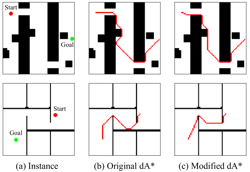
Figure 3: The comparison of the original dA^∗ and the modified dA^∗. (a) displays the selected instances with map, start node (red), and goal node (green). (b) and (c) presents the pathfinding results generated by the original dA^∗ and the modified dA^∗.

V-B Benchmarks

To evaluate the performance of the proposed iA^∗ framework in the search-based pathfinding, we selected the latest open-source data-driven search-based pathfinding methods, Neural A^∗ [10], Focal Search with Path Probability Map (FS + PPM) and Weighted A^∗ + correction factor (WA^∗ + CF) [11], as competitors. Besides, we also select the Weighted A^∗ [42] as a classical competitor that finds the near-optimal path to improve search efficiency. The Neural A^∗, FS + PPM, and WA^∗ + CF have been trained by the MP dataset in a supervised fashion, and we use the well-trained parameters published on their website. Besides, we train our instance encoder within iA^∗ using the same dataset. FS + PPM and WA^∗ + CF only support the map with a fixed shape, $64\times 64$, as their input because of their network designs with constraints on the input shape. Thus, we only assess the performance of these two methods with the $64\times 64$ maps.

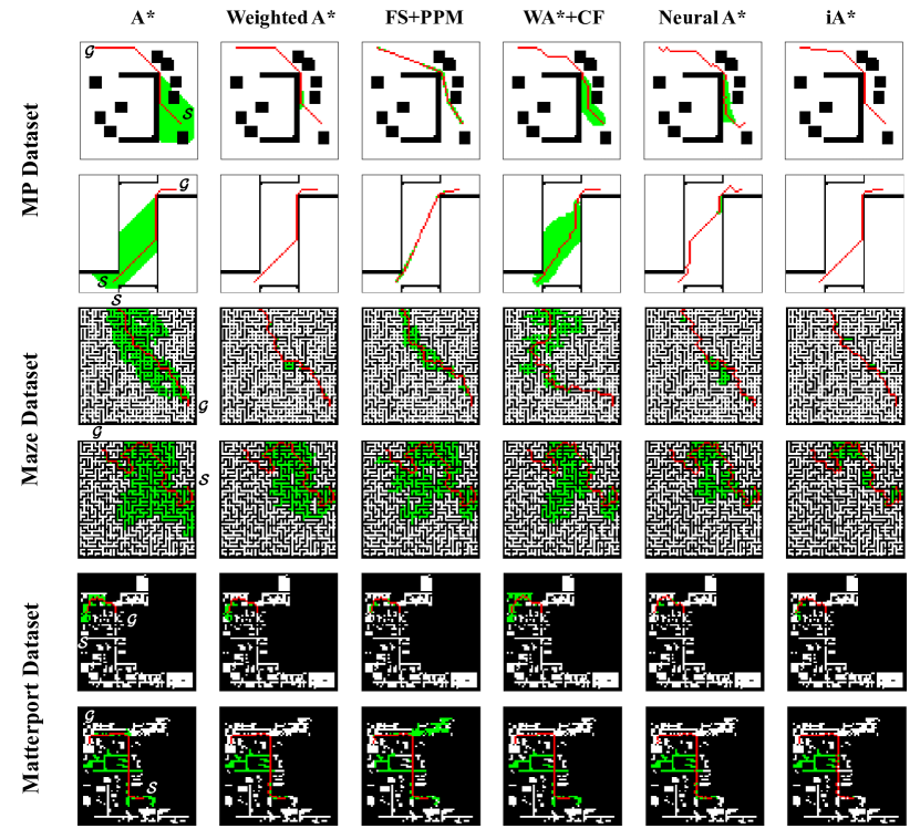
Figure 4: Selected pathfinding results of different methods in the three datasets, MP dataset (the first two rows), Maze dataset (the middle two rows), and Matterport dataset (the last two rows). $\bm{\mathcal{S},\mathcal{G}}$ indicate the start node and goal node in the given map, respectively. The pathfinding results are indicated as red pixels, while the green pixels indicate the searched area during pathfinding.

V-C Metrics

To evaluate the performance of the proposed method and compare it with other methods, we mainly use the following metrics to compare their search efficiency.

• Reduction ratio of node explorations (Exp) [10]: To measure the search efficiency of the examined method, we utilize the ratio of the reduced search area to the classical A^∗ search as a metric, which is defined as

  $$\textit{Exp}=100\times\frac{S^{*}-S}{S^{*}},$$ (9)

  where $S$ represents the search area of the examined method and $S^{*}$ is the search area of classical A^∗ search.

• Reduction ratio of time (Rt): To measure the time efficiency of the examined method, we utilize the ratio of saved time to the operation time of standard A^∗ search as a metric, which is defined as

  $$\textit{Rt}=100\times\frac{t^{*}-t}{t^{*}},$$ (10)

  where $t^{*}$ is the operating time of classical A^∗ solution, and $t$ is the operating time of the examined method.

V-D Test in Datasets

DA^∗

To evaluate the modification of differentiable A^∗, we compare the paths generated by original dA^∗ [10] and the modified dA^∗. We use the MP dataset for evaluation, and the results are shown in Fig. 3. From the results, it is observed that the original dA^∗ fails to find the shortest paths with given instances, while the modified dA^∗ can guarantee finding the optimal path. Given the importance of a closed-form solution in lower-level optimization, we choose the modified dA^∗.

Comparisons with Benchmarks

To display the performance of iA^∗, we conduct both qualitative and quantitative experiments, and the results are separately shown in Fig. 4 and Tab. I. Fig. 4 visualizes the pathfinding results of the selected methods. From the results, the proposed iA^∗ can greatly reduce the search area and still get paths similar to optimal paths generated by classical A^∗. For detailed comparisons, Table I summarizes the quantitative experimental results in the MP, Maze, and Matterport3D datasets. The results demonstrate the pathfinding performance in the map with different shapes with the mentioned metrics. In MP Dataset, the FS-PPM algorithm has the overwhelming performance in both Exp and Rt metrics. However, in the other two datasets, the FS-PPM algorithm performs poorly, even searching more areas and spending more time. In the experiments of the Maze dataset, the FS + PPM even increases 105% operation time and 8% search area, compared with the classical A^∗ search. Therefore, it is likely that FS + PPM is overfitting on the MP dataset. If we exclude the FS-PPM from consideration, the proposed iA^∗ demonstrates superior performance of search efficiency on this dataset among the rest of the selected methods. Besides, iA^∗ also has a satisfactory performance in the remaining two datasets. The experimental results display that iA^∗ is effective in reducing the search time and improving the efficiency of pathfinding. Even in large environments, the proposed iA^∗ outperforms classical and data-driven methods. Additionally, the near-optimal paths generated by iA^∗ only have a 3.45% to 4.64% increase in path length. In summary, the proposed iA^∗ can improve the pathfinding efficiency in various environments.

TABLE I: Experimental Results in the Selected Datasets

MP Dataset
	$64\times 64$		$128\times 128$		$256\times 256$
	Exp	Rt	Exp	Rt	Exp	Rt
WA∗	63.5%	47.0%	70.1%	55.4%	52.0%	54.4%
Neural A∗	56.0%	24.5%	67.2%	42.1%	44.9%	50.0%
WA∗+CF	68.8%	48.0%	/	/	/	/
FS+PPM	88.3%	83.6%	/	/	/	/
iA∗ (Ours)	69.4%	52.8%	75.9%	62.3%	56.1%	61.5%

Maze Dataset
	$64\times 64$		$128\times 128$		$256\times 256$
	Exp	Rt	Exp	Rt	Exp	Rt
WA∗	21.7%	27.4%	48.8%	11.7%	41.8%	29.5%
Neural A∗	30.9%	40.8%	60.5%	32.8%	51.0%	38.9%
WA∗+CF	47.3%	45.3%	/	/	/	/
FS+PPM	-8.9%	-105.0%	/	/	/	/
iA∗ (Ours)	37.8%	44.9%	64.8%	33.0%	51.5%	63.9%

Matterport3D Dataset
	$64\times 64$		$128\times 128$		$256\times 256$
	Exp	Rt	Exp	Rt	Exp	Rt
WA∗	48.1%	36.8%	76.4%	79.6%	84.7%	81.5%
Neural A∗	42.3%	28.4%	65.6%	50.1%	79.4%	63.9%
WA∗+CF	57.2%	42.7%	/	/	/	/
FS+PPM	9.3%	-43.8%	/	/	/	/
iA∗ (Ours)	57.8%	44.7%	79.2%	81.8%	89.5%	87.8%

TABLE II: Quantitative Results in the Simulated Environments

		A∗	Neural A∗	iA∗
Indoor	Exp (Area)	0 (9826)	3.95% (9438)	43.28% (5573)
	Rt (Time)	0 (3.11 s)	3.67% (2.99 s)	52.04% (1.49 s)
	Length	374.044	385.878	379.114
Tunnel	Exp (Area)	0 (45763)	13.37% (39643)	62.73% (17054)
	Rt (Time)	0 (14.31 s)	14.99% (12.16 s)	62.84% (5.31 s)
	Length	801.018	822.234	809.4

V-E Test in Simulation Environments:

To validate the practicality of iA^∗, we evaluate the pathfinding methods in the widely used Autonomous Exploration Development Environment [43] that includes a mobile robot and several simulated scenarios resembling real-world settings. We select two of them as our test environments, the indoor and the tunnel scenarios, shown as Fig. 5 (a). The simulation environments only provide dense point cloud maps. Thus, we need to transform them into two-dimensional binary maps. Specifically, we first define the resolution of binary maps as $0.5\mathrm{m}$, which means that each grid cell in the binary map represents a $0.5\mathrm{m}\times 0.5\mathrm{m}$ area in the xy-plane of the original map. Then, all the points in the point cloud map are mapped into their respective grid cells. If the maximum z-value of points exceeds a given threshold in one grid cell, this grid cell will be regarded as an obstacle cell. If otherwise, this grid cell will be a free one. Ultimately, we get the maps of the Tunnel and Indoor scenarios, with shapes of $654\times 505$ and $259\times 199$, respectively. In this way, the shapes of the generated maps are different. Thus, the Neural A^∗ pathfinding is the only data-driven method that can use them as input except ours, so we mainly compare the performances between Classical A^∗, Neural A^∗, and iA^∗.

Then, the simulation experiment is conducted to navigate a mobile robot to the given goals. The start position is the position of the mobile robot, and a goal position is given. After finding the path, we use the integrated path-following tool within the simulation environment to provide control commands for the mobile robot to navigate. From the experimental results in Fig. 5, both Neural A^∗ and iA^∗ can generate obstacle-free paths, similar to the optimal path generated by Classical A^∗, and allow the robot to finish the navigation task successfully. For a detailed comparison, the quantitative analysis is conducted to assess their search efficiency in robot navigation tasks by Length (Eq. (7)), Exp (Eq. (9)) and Rt (Eq. (10)) metrics. The results are shown in Table II. It is seen that the proposed iA^∗ significantly improves the pathfinding efficiency. Specifically, in the Indoor scenario, iA^∗ reduces 43.28% search area and saves 52.04% time with only a sight increase of about 1.36% in path length; in the Tunnel scenario, it reduces 62.73% search area and saves 62.84% time with 1.04% increase in length.

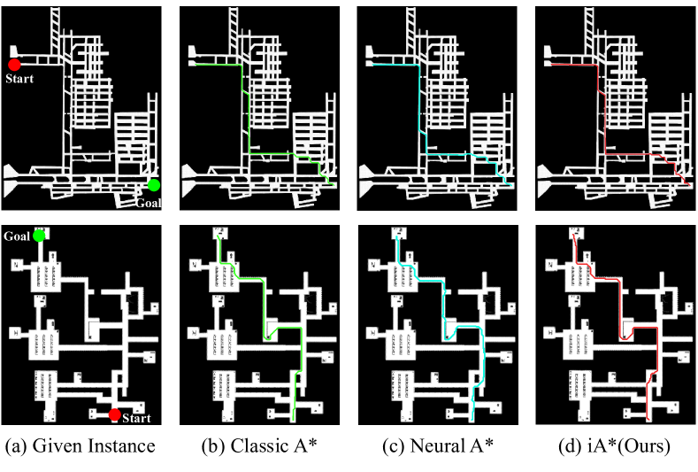
Figure 5: The trajectories of a mobile robot under given navigation tasks in the simulation environments, Tunnel (the first row) and Indoor (the second row). (a) represents the given instances, start (red circle), and goal (green circle). (b), (c) and (d) represent the trajectories of a mobile robot navigating from start to goal in the simulation environments with Classical A^∗, Neural A^∗, and iA^∗.

VI Conclusion

To summarize, we propose iA^∗, a novel search-based pathfinding framework that adopts the imperative learning strategy to improve the pathfinding efficiency. We formulate the iA^∗ as a bilevel optimization, where the upper-level optimization narrows the search space using an instance encoder while the lower-level optimization is the A^∗ search algorithm to generate the optimal solution. To avoid data labeling, the encoder is trained in a self-supervised manner that calculates loss from the results of low-level optimization. Moreover, the instance encoder is designed as a fully convolutional network that supports different input shapes, ensuring that iA^∗ can be applied to various environments. In the experiments, we assess iA^∗ with public datasets and simulation environments. From the experimental results, it is observed that the proposed iA^∗ outperforms the selected data-driven pathfinding methods on pathfinding efficiency and can achieve robot navigation tasks in diverse environments.

References

- [1] B. Patle, A. Pandey, D. Parhi, A. Jagadeesh, et al., “A review: On path planning strategies for navigation of mobile robot,” Defence Technology, vol. 15, no. 4, pp. 582–606, 2019.
- [2] L. Quan, L. Han, B. Zhou, S. Shen, and F. Gao, “Survey of uav motion planning,” IET Cyber-systems and Robotics, vol. 2, no. 1, pp. 14–21, 2020.
- [3] E. Dijkstra, “A note on two problems in connexion with graphs,” Numerische Mathematik, vol. 1, no. 1, pp. 269–271, 1959.
- [4] P. E. Hart, N. J. Nilsson, and B. Raphael, “A formal basis for the heuristic determination of minimum cost paths,” IEEE transactions on Systems Science and Cybernetics, vol. 4, no. 2, pp. 100–107, 1968.
- [5] A. Stentz, “Optimal and efficient path planning for partially-known environments,” in Proceedings of the 1994 IEEE International Conference on Robotics and Automation, 1994, pp. 3310–3317 vol.4.
- [6] I. Noreen, A. Khan, and Z. Habib, “Optimal path planning using rrt* based approaches: a survey and future directions,” International Journal of Advanced Computer Science and Applications, vol. 7, no. 11, 2016.
- [7] D. González, J. Pérez, V. Milanés, and F. Nashashibi, “A review of motion planning techniques for automated vehicles,” IEEE Transactions on intelligent transportation systems, vol. 17, no. 4, pp. 1135–1145, 2015.
- [8] V. Bulitko, Y. Björnsson, N. R. Sturtevant, and R. Lawrence, “Real-time heuristic search for pathfinding in video games,” in Artificial Intelligence for Computer Games. Springer, 2011, pp. 1–30.
- [9] S. J. Russell and P. Norvig, Artificial intelligence: a modern approach. Pearson, 2016.
- [10] R. Yonetani, T. Taniai, M. Barekatain, M. Nishimura, and A. Kanezaki, “Path planning using neural a* search,” in International conference on machine learning. PMLR, 2021, pp. 12 029–12 039.
- [11] D. Kirilenko, A. Andreychuk, A. Panov, and K. Yakovlev, “Transpath: learning heuristics for grid-based pathfinding via transformers,” in Proceedings of the AAAI Conference on Artificial Intelligence, vol. 37, no. 10, 2023, pp. 12 436–12 443.
- [12] F. Yang, C. Wang, C. Cadena, and M. Hutter, “iPlanner: Imperative path planning,” in Robotics: Science and Systems (RSS), 2023.
- [13] T. Fu, S. Su, Y. Lu, and C. Wang, “iSLAM: Imperative SLAM,” IEEE Robotics and Automation Letters (RA-L), 2024.
- [14] Z. Zhan, D. Gao, Y.-J. Lin, Y. Xia, and C. Wang, “imatching: Imperative correspondence learning,” arXiv preprint arXiv:2312.02141, 2023.
- [15] R. Liu, J. Gao, J. Zhang, D. Meng, and Z. Lin, “Investigating bi-level optimization for learning and vision from a unified perspective: A survey and beyond,” IEEE Transactions on Pattern Analysis and Machine Intelligence, vol. 44, no. 12, pp. 10 045–10 067, 2021.
- [16] C. Wang, D. Gao, K. Xu, J. Geng, Y. Hu, Y. Qiu, B. Li, F. Yang, B. Moon, A. Pandey, et al., “Pypose: A library for robot learning with physics-based optimization,” in Proceedings of the IEEE/CVF Conference on Computer Vision and Pattern Recognition, 2023, pp. 22 024–22 034.
- [17] D. B. West et al., Introduction to graph theory. Prentice hall Upper Saddle River, 2001, vol. 2.
- [18] J. E. Doran and D. Michie, “Experiments with the graph traverser program,” Proceedings of the Royal Society of London. Series A. Mathematical and Physical Sciences, vol. 294, no. 1437, pp. 235–259, 1966.
- [19] A. Stentz, “Optimal and efficient path planning for partially-known environments,” in Proceedings of the 1994 IEEE international conference on robotics and automation. IEEE, 1994, pp. 3310–3317.
- [20] S. M. LaValle, J. J. Kuffner, B. Donald, et al., “Rapidly-exploring random trees: Progress and prospects,” Algorithmic and computational robotics: new directions, vol. 5, pp. 293–308, 2001.
- [21] S. Karaman and E. Frazzoli, “Sampling-based algorithms for optimal motion planning,” The international journal of robotics research, vol. 30, no. 7, pp. 846–894, 2011.
- [22] J. D. Gammell, S. S. Srinivasa, and T. D. Barfoot, “Informed rrt: Optimal sampling-based path planning focused via direct sampling of an admissible ellipsoidal heuristic,” in 2014 IEEE/RSJ international conference on intelligent robots and systems. IEEE, 2014, pp. 2997–3004.
- [23] J. D. Gammell, T. D. Barfoot, and S. S. Srinivasa, “Batch informed trees (bit*): Informed asymptotically optimal anytime search,” The International Journal of Robotics Research, vol. 39, no. 5, pp. 543–567, 2020.
- [24] M. P. Strub and J. D. Gammell, “Adaptively informed trees (ait): Fast asymptotically optimal path planning through adaptive heuristics,” in 2020 IEEE International Conference on Robotics and Automation (ICRA). IEEE, 2020, pp. 3191–3198.
- [25] “Path planning using lazy prm,” in Proceedings 2000 ICRA. Millennium conference. IEEE international conference on robotics and automation. Symposia proceedings (Cat. No. 00CH37065), vol. 1. IEEE, 2000, pp. 521–528.
- [26] A. A. Ravankar, A. Ravankar, T. Emaru, and Y. Kobayashi, “Hpprm: hybrid potential based probabilistic roadmap algorithm for improved dynamic path planning of mobile robots,” IEEE Access, vol. 8, pp. 221 743–221 766, 2020.
- [27] C. Liu, S. Xie, X. Sui, Y. Huang, X. Ma, N. Guo, and F. Yang, “Prm-d* method for mobile robot path planning,” Sensors, vol. 23, no. 7, p. 3512, 2023.
- [28] S. Choudhury, M. Bhardwaj, S. Arora, A. Kapoor, G. Ranade, S. Scherer, and D. Dey, “Data-driven planning via imitation learning,” The International Journal of Robotics Research, vol. 37, no. 13-14, pp. 1632–1672, 2018.
- [29] T. Takahashi, H. Sun, D. Tian, and Y. Wang, “Learning heuristic functions for mobile robot path planning using deep neural networks,” in Proceedings of the International Conference on Automated Planning and Scheduling, vol. 29, 2019, pp. 764–772.
- [30] O. Ronneberger, P. Fischer, and T. Brox, “U-net: Convolutional networks for biomedical image segmentation,” in Medical Image Computing and Computer-Assisted Intervention–MICCAI 2015: 18th International Conference, Munich, Germany, October 5-9, 2015, Proceedings, Part III 18. Springer, 2015, pp. 234–241.
- [31] A. Vaswani, N. Shazeer, N. Parmar, J. Uszkoreit, L. Jones, A. N. Gomez, Ł. Kaiser, and I. Polosukhin, “Attention is all you need,” Advances in neural information processing systems, vol. 30, 2017.
- [32] J. Wang, W. Chi, C. Li, C. Wang, and M. Q.-H. Meng, “Neural rrt*: Learning-based optimal path planning,” IEEE Transactions on Automation Science and Engineering, vol. 17, no. 4, pp. 1748–1758, 2020.
- [33] A. H. Qureshi, Y. Miao, A. Simeonov, and M. C. Yip, “Motion planning networks: Bridging the gap between learning-based and classical motion planners,” IEEE Transactions on Robotics, vol. 37, no. 1, pp. 48–66, 2020.
- [34] L. P. Kaelbling, M. L. Littman, and A. W. Moore, “Reinforcement learning: A survey,” Journal of artificial intelligence research, vol. 4, pp. 237–285, 1996.
- [35] A. I. Panov, K. S. Yakovlev, and R. Suvorov, “Grid path planning with deep reinforcement learning: Preliminary results,” Procedia computer science, vol. 123, pp. 347–353, 2018.
- [36] P. Gao, Z. Liu, Z. Wu, and D. Wang, “A global path planning algorithm for robots using reinforcement learning,” in 2019 IEEE International Conference on Robotics and Biomimetics (ROBIO). IEEE, 2019, pp. 1693–1698.
- [37] R. A. Horn and C. R. Johnson, Matrix analysis. Cambridge university press, 2012.
- [38] J. Long, E. Shelhamer, and T. Darrell, “Fully convolutional networks for semantic segmentation,” in Proceedings of the IEEE conference on computer vision and pattern recognition, 2015, pp. 3431–3440.
- [39] M. Bhardwaj, S. Choudhury, and S. Scherer, “Learning heuristic search via imitation,” in Conference on Robot Learning. PMLR, 2017, pp. 271–280.
- [40] M. I. Ivanitskiy, R. Shah, A. F. Spies, T. Räuker, D. Valentine, C. Rager, L. Quirke, C. Mathwin, G. Corlouer, C. D. Behn, et al., “A configurable library for generating and manipulating maze datasets,” arXiv preprint arXiv:2309.10498, 2023.
- [41] A. Chang, A. Dai, T. Funkhouser, M. Halber, M. Niebner, M. Savva, S. Song, A. Zeng, and Y. Zhang, “Matterport3d: Learning from rgb-d data in indoor environments,” in 2017 International Conference on 3D Vision (3DV). IEEE Computer Society, 2017, pp. 667–676.
- [42] I. Pohl, “Heuristic search viewed as path finding in a graph,” Artificial intelligence, vol. 1, no. 3-4, pp. 193–204, 1970.
- [43] C. Cao, H. Zhu, F. Yang, Y. Xia, H. Choset, J. Oh, and J. Zhang, “Autonomous exploration development environment and the planning algorithms,” in 2022 International Conference on Robotics and Automation (ICRA), 2022, pp. 8921–8928.