Initialisation and Topology Effects in Decentralised Federated Learning

Abstract

Fully decentralised federated learning enables collaborative training of individual machine learning models on distributed devices on a network while keeping the training data localised. This approach enhances data privacy and eliminates both the single point of failure and the necessity for central coordination. Our research highlights that the effectiveness of decentralised federated learning is significantly influenced by the network topology of connected devices. A simplified numerical model for studying the early behaviour of these systems leads us to an improved artificial neural network initialisation strategy, which leverages the distribution of eigenvector centralities of the nodes of the underlying network, leading to a radically improved training efficiency. Additionally, our study explores the scaling behaviour and choice of environmental parameters under our proposed initialisation strategy. This work paves the way for more efficient and scalable artificial neural network training in a distributed and uncoordinated environment, offering a deeper understanding of the intertwining roles of network structure and learning dynamics.

1 Introduction

The traditional centralised approach to machine learning has shown great promise and has seen considerable progress in the last few decades. This approach, while practical, comes at a cost in terms of systemic data privacy risks and centralisation overhead (McMahan et al., 2017; Kairouz et al., 2021; Rieke et al., 2020). To alleviate these issues, the federated learning framework was proposed where each node (client) updates a local machine learning model using local data and only shares its model parameters with a centralised server, which in turn aggregates these individual models into one model and redistributes it to each node (McMahan et al., 2017).

While this approach reduces the data privacy risk by eliminating data sharing with the centralised server, it still maintains a singular point of failure and puts a heavy communication burden on the central server node (Beltrán et al., 2023; Lalitha et al., 2018). Decentralised federated learning aims to provide an alternative approach that maintains data privacy but removes the need for a centralised server. This involves the set of nodes (clients) updating their local models based on the local data, but directly communicating with one another through a communication network. Each node then updates its local model by aggregating those of the neighbourhood (Beltrán et al., 2023; Valerio et al., 2023). The efficiency of this approach is impacted by several kinds of inhomogeneities (Valerio et al., 2023) characterising the network structure, initial conditions, learning data, and temporal irregularities. In this paper, we focus on the first two of these.

Motivation.

Decentralised federated learning immediately raises two distinct new issues compared to the centralised federated learning approach. First, that the initialisation and operations of the nodes have to be performed in an uncoordinated manner, as the role of coordination previously lay with the server. Second, that the effect of structure and possible heterogeneities in the communication network structure is poorly understood. In the case of centralised federated learning, the communication network is organised as a simple star graph. In a decentralised setting, however, the network might be an emergent result of, e.g., the social network of the users of the devices, a distributed peer-discovery protocol or a hand-engineered topology comprising of IoT devices. Each of these assumptions leads to a different network topology with wildly different characteristics. Many network topologies modelling real-world phenomena, unlike a star graph, have diameters that monotonically scale up with the number of nodes, inducing an inherent latency in the communication of information between nodes that are not directly connected. Structural heterogeneities, e.g., the dimensionality of the network, degree heterogeneity and heterogeneities in other centrality measures also play important roles in the evolution of the information-sharing processes on networks. This makes network heterogeneities primary candidates for analysis of any decentralised system.

Contribution.

In this manuscript, we focus on these two issues: we show that without prior coordination the standard method of artificial neural network initialisation results in subpar performance when training deep neural networks, and propose an alternative uncoordinated neural network initialisation method to resolve this issue. We then present an analysis of the effect of network topology on the proposed initialisation process and demonstrate how it affects the scaling properties of the system.

2 Related works

Decentralised federated learning (Beltrán et al., 2023) comes as a natural next step in the development of the field of federated learning since the introduction of this method (McMahan et al., 2017). This approach has been used in application areas such as object recognition in medical images (Roy et al., 2019; Tedeschini et al., 2022) and other industrial settings (Savazzi et al., 2021; Qu et al., 2020). It also has been extended with novel optimisation and aggregation methods (Sun et al., 2022; Lalitha et al., 2018).

The structure of complex networks, central to federated learning by coding the communication structure between connected devices, can embody various heterogeneities. They have been found to be a crucial factor in understanding a variety of complex systems that involve many entities communicating or interacting together. For example, the role of degree distribution (Jennings, 1937; Albert et al., 2000), high clustering (Watts & Strogatz, 1998; Luce & Perry, 1949) or existence of flat or hierarchical community structures (Rice, 1927; Fortunato & Hric, 2016) in networks of real-world phenomena has been understood and analysed for decades. Recent advances in network modelling have extended heterogeneities in networks from structural to incorporate spatial (Orsini et al., 2015) and also temporal heterogeneities, induced by patterns of, e.g., spatial constraints or bursty or self-exciting activity of the nodes (Karsai et al., 2011; Gauvin et al., 2022; Badie-Modiri et al., 2022a, b). In the decentralised federated learning settings, the matter of structural heterogeneities of the underlying communication network has only been very recently subjected to systemic studies. Notably, Vogels et al. (2022) analyse the effect of topology on optimal learning rate and Palmieri et al. (2023) analyse the differences among individual training curves of specific nodes (e.g., high-degree hubs versus peripheries) for Barabási–Albert networks and stochastic block models with two blocks (Newman, 2010).

On the matter of parameter initialisation in federated learning, recent studies have focused on the effect of starting all nodes from a homogeneous set of parameters (Valerio et al., 2023) or the parameters of an independently pre-trained model (Nguyen et al., 2022). Historically, artificial neural networks were initialised from random uniform or Gaussian distribution with scales set based on heuristics and trial and error (Goodfellow et al., 2016) or for specific activation functions (LeCun et al., 2002). The advent of much deeper architectures and widespread use of non-linear activation functions such as ReLU or Tanh led to a methodical understanding of the role of initial parameters to avoid exploding or diminishing activations and gradients. Glorot & Bengio (2010) proposed a method based on certain simplifying assumptions about the non-linearities used. Later, He et al. (2015) defined a more general framework for use with a wider variety of non-linearities, which was used for training the ResNet image recognition model (He et al., 2016).

In this work, we will be extending the same approach for effective initialisation of artificial neural network parameters to the decentralised setting, where the parameters are not only affected by the optimisation based on the training data but also due to interactions with other nodes of the communication network.

3 Preliminaries

In our setup, we used a simple decentralised federated learning system with an iterative process. All nodes use the same artificial neural network architecture. Nodes are connected through a predetermined static, undirected communication network $G$. Nodes initialise their local model parameters based on one of the following strategies: (1) homogeneous initialisation, a coordinated approach where all nodes use the same set of predetermined parameters, (2) random initialisation with no gain correction, an uncoordinated approach where each node draws their initial parameters independently based on a strategy optimised for isolated centralised training, e.g., from He et al. (2015), or (3) random initialisation with gain correction, which is our proposed initialisation strategy that re-scales initial parameter distributions from (2) based on the topology of the communication network of nodes. This approach will be explored in detail in Section 4.

Additionally, each node is assigned a specific exclusive set of labelled items as its private training data. Each node can access its private data but not those of other nodes. The data each node has access to does not change over time and no two nodes get access to the same item. In this work, each node gets access to an equal subset of items belonging to each class, randomly selected at the beginning of the simulation. For measuring the performance of the system, a subset of data not assigned to any node is reserved for testing. To isolate the network effects from data effects, we chose a simple setting where the data is iid among nodes and balanced across labels. It is likely that the non-iid data would be correlated with network features, which would make it difficult to isolate the network effects. We believe that the interactions between data and label distribution and the network features and topology would prove an important line of future research on this topic.

At each iteration, called here a communication round, nodes update their parameters (weights and biases) to the mean value calculated across their neighbourhood. They then perform one unit of local training, performing a set number of epochs of training on their local data using a simple stochastic gradient descent optimiser. The artificial neural network architecture employed in this manuscript is a simple feedforward neural network with four fully connected layers, consisting of 512, 256, and 128 neurons in three hidden layers, followed by an output layer of size 10, and employs ReLU activation functions after each layer except the output layer. Our experiments will be performed on subsets of the MNIST digit classification task (LeCun et al., 1998), distributed equally between the nodes. Of course, the effects of the initialisation method would be even more visible in deeper neural network architectures (He et al., 2015; Glorot & Bengio, 2010).

Note that the centralised federated learning using the simple parameter averaging aggregation method (FedAvg) can be viewed as a special case of the decentralised federated learning using the simple averaging aggregation (DecAvg) on a fully connected network, as at each step each node concurrently plays the role of the central server, setting its parameters to the average parameters of all other nodes. This means that to the extent that the results presented in this manuscript apply to fully connected networks, they can be utilised to understand the behaviour of this configuration of a centralised federated learning process as well.

Here is a brief description of the notation used in this manuscript: When referring to the communication network (graph), $n$ indicates the number of nodes (sometimes referred to as the system size), while $k_{i}$ indicates the degree of a node $i$ defined as the number of its neighbours, and $p(k)$ is the degree distribution. For a node that is reached by following a random link, $q(k)$ is the distribution of the number of other links to that node, known as the excess degree distribution of the graph. The adjacency matrix is indicated by $A$. $d$ shows the number of dimensions of $d$-dimensional tori.

Expected values are indicated using the brackets around the random variable, e.g., $\langle k\rangle$ is the mean degree. Standard deviation is shown using $\sigma(...)$. The $p$ parameters of node $i$ are indicated by vector $w_{i}$ of size $p$, sometimes arranged in a $p\times n$ matrix $W$. $\sigma_{ap}$ indicates mean standard deviation across columns of $W$, i.e. expected value of standard deviation of parameters of the same node, while $\sigma_{an}$ indicates mean standard deviation across rows, which is the expected standard deviation of the same parameter between nodes. Artificial neural networks are usually initialised with parameters that are drawn from different sets of distribution, e.g., weights of each layer are drawn from a separate distribution. In this case, a vector $w_{i}$ can be formed for one specific set of parameters, drawn from a distribution with standard deviation $\sigma_{init}$.

4 Uncoordinated artificial neural network initialisation

Unlike in centralised federated learning, it is unwarranted to assume that in a massive decentralised federated learning setup, all nodes can negotiate and agree on initial values for model parameters. A fully uncoordinated method for selecting initial values for the model parameters means that each node should be able to draw initial values for their model parameters independently with no communication.

It has been shown that judicious choice of initialisation strategy can enable training of much deeper artificial neural networks (Glorot & Bengio, 2010; He et al., 2015, 2016). Specifically, a good parameter initialisation method leads to initial parameters that neither increase nor decrease activation values for consecutive layers exponentially (He et al., 2015; Glorot & Bengio, 2010). In the case of decentralised federated learning, this proves more challenging, as the aggregation step changes the distribution of parameters, meaning that the optimal initial value distributions are not only a function of the machine learning model architecture, but also affected by the communication network structure.

Empirically, we observe (Figure 1(a) dashed lines) that the decentralised, uncoordinated initialisation of nodes using the method proposed by  He et al. (2015) results in progressively poorer performance in the federated setting as the number of nodes grows, while the proposed uncoordinated initialisation performs similarly to the coordinated homogeneous strategy. Figure 1(b) shows this as a linear scaling of the loss trajectory as a function of communication rounds with the number of nodes.

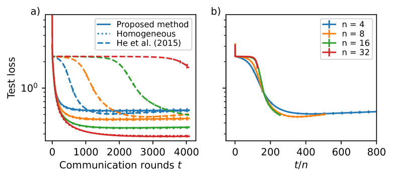
Figure 1: Mean test cross-entropy loss with the proposed initialisation compared to coordinated homogeneous initialisation and the initialisation method proposed in He et al. (2015) without re-scaling. The decentralised federated learning process on nodes connected through a fully-connected (complete) network of various sizes, with 8 training samples of each digit per node, 1 epoch per communication round. The results show that without the proposed re-scaling of the parameters, the mean test loss has a plateau lasting a number of rounds linear to the system size, while our uncoordinated proposed initialisation method performs on par with the coordinated homogeneous initialisation. Panel (b) shows the linear scaling of the test loss time trajectory of the independent (He et al., 2015) method initialisation with system size. Error bars represent 95% confidence intervals.

To understand the general characteristics of the learning process we propose a simplified numerical model: an iterative process, where each of the $n$ network nodes has a vector of $p$ parameters drawn from a normal distribution with standard deviation $\sigma_{\text{init}}$. At each iteration, similar to the federated averaging step, each node updates its parameter vector by averaging its immediate neighbourhood, then, to mimic the effects of the local training step all node parameters are updated by adding a normally distributed noise with standard deviation $\sigma_{\text{noise}}$.

This model mimics the general behaviour of the decentralised learning system at the early stages of the process, since we can assume that the changes to the parameters as a result of the local learning process are generally negligible compared to the changes in parameters due to the aggregation steps. Simulations of the decentralised federated learning process (Figure 2) can provide evidence for this assumption. The implementation of the simulated decentralised federated learning system is available for the purposes of reproduction under the MIT open-source license at https://github.com/arashbm/gossip_training.

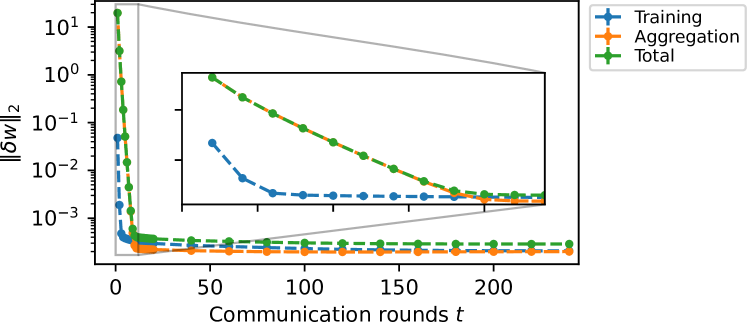
Figure 2: Mean magnitude of change in parameters due to the training and aggregation independently as well as the total change. In the early rounds of the iterative process, the vector of change due to the aggregation is several orders of magnitude larger than that of the training. This, combined with the cosine similarity plot from Figure 4(b) showing the orthogonality of these vectors in the early rounds, supports the numeric model assumption that the early evolution of the system is dominated by the aggregation step. Changes were calculated by simulating the decentralised federated learning process on 256 nodes, connected through a random 32-regular network, with 8 training samples of each digit per node, 1 epoch per communication round. Error bars represent 95% confidence intervals.

The results from the simplified numeric model for random $k$-regular graphs predict, as shown in Figure 4, that the standard deviation of the value of the same parameter across nodes averaged for all parameters, which we call $\sigma_{an}$, will decrease to some value close to the standard deviation of noise (simulating changes due to local training). Meanwhile the standard deviation of the parameters of the same node average across all nodes, $\sigma_{ap}$, will decrease only to a factor of $1/\sqrt{n}$ of the original standard deviation $\sigma_{\text{init}}$. Note that for artificial neural networks each layer’s initial weights and biases are usually drawn from distributions with different values of $\sigma_{\text{init}}$, based on the number of inputs and outputs of each layer and other considerations. The analysis here can be applied to each batch of parameters drawn from the same distribution, e.g., to weights of the same layer, independently. A schematic visualisation of the aggregation process with definitions of $\sigma_{an}$ and $\sigma_{ap}$ is provided in Figure 3.

Figure 3: Schematic representation of the decentralised federated learning as presented in this work, as well as the numeric model used in Section 4. At each step, each node individually updates its parameters based on performing optimisation on local training data in case of the real decentralised federated learning process or by simply adding a random noise vector drawn from a Gaussian distribution with standard deviation $\sigma_{\text{noise}}$ for the numerical model. Each node then aggregates all parameters from its neighbourhood through simple averaging, i.e., $w_{u}\leftarrow\sum_{v\in N(u)}w_{v}/|N(u)|$ where $N(i)$ is the immediate neighbourhood of node $i$, including $i$ itself. The characteristic standard deviations are defined as $\sigma_{ap}=\sum_{v\in G}\sigma(w_{v})/n$ and $\sigma_{an}=\sum_{q=1}^{p}\sigma(W_{q*})/p$.

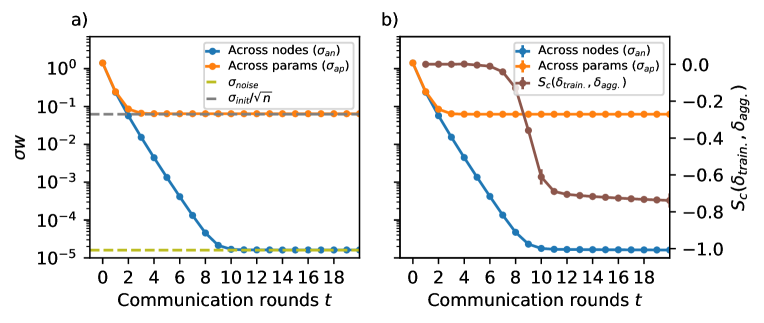
Figure 4: Evolution of standard deviation of a single parameter across all nodes $\sigma_{an}$ as well the mean standard deviation of parameters in each node $\sigma_{ap}$ from (a) the numerical simplified model and (b) simulation of the distributed learning process. Both were carried out on a random 32-regular network with $n=512$. The simplified numerical model uses $p=200$ parameters per node and the distributed learning models use a sample of the second linear layer weights. The simulations were run with 8 instances of each digit per node as training data. Furthermore, the trajectory of cosine similarity of the vectors of change in parameters due to training and aggregation $S_{c}(\delta_{\text{train.}},\delta_{\text{agg.}})$ indicates that for the duration of the stabilisation phase, the two vectors are mostly orthogonal. Error bars in panel (b) represent 95% confidence intervals.

From the dynamics visualised in Figure 4, two in particular stand out due to their important role in understanding and exploiting the decentralised system. First, the value to which $\sigma_{ap}$ approaches towards can allow us to select the initial distribution of parameters $\sigma_{\text{init.}}$ in a way that after stabilisation of $\sigma_{ap}$, the neural network models would on expectation have an optimal parameter distribution. In Section 4.1, we show that this compression can be calculated for any graph based on the distribution of eigenvector centralities of the nodes (Newman, 2010), with the case of graphs with uniform centralities giving a factor of $1/\sqrt{n}$. Second, the time to reach the steady state for $\sigma_{an}$ plays an important role since this determines the number of rounds required for the heterogeneous initial condition before the improvements of the learning process start in earnest. This is because the magnitude of the changes to parameters due to the learning process (modelled by noise in the numerical model) becomes comparable to those of the aggregation process. In Section 4.2 we show that this “stabilisation” time scales similar, up to a constant factor, to the mixing time of lazy random walks on the graph.

4.1 The compression of node parameters

We can analytically estimate the steady state values for $\sigma_{an}$ and $\sigma_{ap}$, as well as the scaling of the number of rounds to arrive at these values using methods from finite-state discrete-time Markov chains. Let $A$ be the adjacency matrix of our underlying graph $G$. We construct a right stochastic matrix $A^{\prime}$ where

$$A^{\prime}_{ij}=\frac{A_{ij}+I_{ij}}{\sum_{k}A_{kj}+I_{kj}}\,,$$ (1)

where $I_{kj}=\delta_{kj}$ are the elements of an identity matrix $I$. This corresponds to the Markov transition matrix of random walks on graph $G$, if the random walker can stay at the same node or take one of the links connected to that node with equal probability for each possible action. If we arrange all initial node parameters in a $p\times n$ matrix $W_{\text{init}}$, the parameters at round $t$ are determined by $W_{\text{init}}A^{\prime t}+\sum^{t-1}_{i=0}N_{i}A^{\prime i}$, where $N_{i}$ is a random $p\times n$ noise matrix with each index drawn from $\mathcal{N}(0,\sigma_{\text{noise}}^{2})$.

Assuming that the graph $G$ is connected, the matrix $A^{\prime t}$ would converge to a matrix where each row is the steady state vector of the Markov matrix $A^{\prime}$, the eigenvector corresponding to the largest eigenvalue 1, normalised to sum to 1. If the steady state vector is given as $v_{\text{steady}}$ the variance contribution of the term $W_{\text{init}}A^{\prime t}$ along each row (i.e., expected variance of parameters of each node) is given as $\sigma_{\text{init}}^{2}\left\|v_{\text{steady}}\right\|^{2}$. It can be trivially shown, from a direct application of the Cauchy–Schwarz inequality:

$$|\langle\vec{1},v_{\text{steady}}\rangle|\leq\|\vec{1}\|\|v_{\text{steady}}\|\,,$$ (2)

that given that for connected networks $\langle\vec{1},v_{\text{steady}}\rangle=\sum v_{\text{steady}}=1$, the $\left\|v_{\text{steady}}\right\|^{2}$ term has a minimum value of $1/n$. This is achieved for random regular networks and other network models where nodes have uniformly distributed eigenvector centralities, such as Erdős–Rényi networks and lattices on $d$-dimensional tori.

Given that the noise values are drawn independently, the variance contribution of the noise term $\sum_{i=0}^{t-1}N_{i}A^{\prime i}$ has an upper-bound of $t\sigma^{2}_{\text{noise}}$. If $t\sigma^{2}_{\text{noise}}\ll\sigma^{2}_{\text{init}}/n$, then the standard deviation across parameters at round $t$ can be approximated by

$$\lim_{t\rightarrow\infty}\sigma_{ap}\approx\sigma_{\text{init}}\left\|v_{\text{steady}}\right\|\,.$$ (3)

For a large connected random $k$-regular network, this reduces to $\lim_{t\rightarrow\infty}\sigma_{ap}=\sigma_{\text{init}}/\sqrt{n}$. Generally for other networks, numerical solution for $\left\|v_{\text{steady}}\right\|$ can be obtained by calculating eigenvector centralities of the original network after adding self-loops to all nodes.

These results, combined with the existing analyses on the role of artificial neural network parameters and their effect on diminishing or exploding gradients (He et al., 2015) suggest that it is reasonable to take into account the compression of the node parameters (e.g., the $1/\sqrt{n}$ factor for random regular networks) when initialising the parameters. Depending on the choice of architecture and optimiser, and especially for large networks with hundreds of nodes, this optimal selection of initial parameters can play a sizeable role in the efficacy of the training process. In our experiments, we took this into account by multiplying a gain factor of $\sqrt{n}$ in the standard deviation of layer weights suggested by  He et al. (2015).

Note that the vector $v_{\text{steady}}$ is simply the sum-normalised vector of eigenvector centralities of the communication network nodes with a self-loop added to all nodes, i.e. each element specifies the probability of a random walk to end up on that specific node, if the random walk process has equal probability of taking any of the edges or staying on the node. This means that the value of this gain is a factor of the system size and the distribution of network centralities. This is illustrated in Figure 5 where the value of the scaling factor $\left\|v_{\text{steady}}\right\|$ is shown for Erdős–Rényi, $k$-regular, Barabási–Albert and heavy-tail ($\gamma=-3$) degree distribution configuration model random networks with the same size and (on expectation) the same number of links.

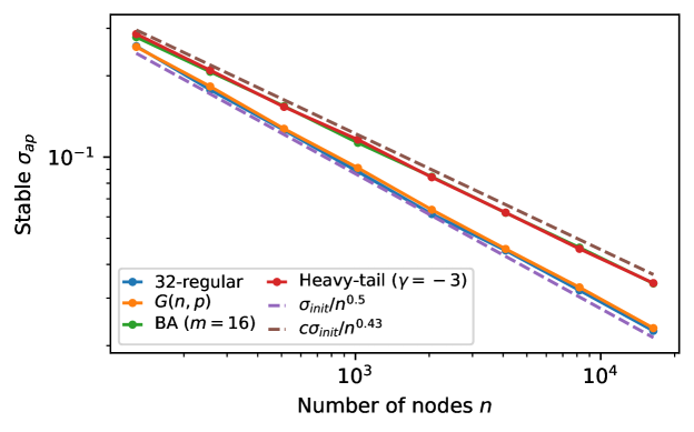
Figure 5: The effect of heterogeneous distribution of centralities in the scaling factor $\left\|v_{\text{steady}}\right\|$ from the simplified numerical model. Homogeneous random networks (Erdős–Rényi $G(n,p)$ networks and random $k$-regular networks) display $\left\|v_{\text{steady}}\right\|=1/\sqrt{n}$, while Barabási–Albert networks and configuration model heavy-tail degree distribution networks ($\gamma=-3$) show this factor scaling exponentially with the number of nodes with a different exponent. Fitted dashed lines are slightly shifted vertically for visibility.

The numeric model applies with minimal changes to directed and weighted communication networks. similar to connected undirected networks. In the case of a strongly connected directed network, the convergence is guaranteed since the stochastic matrix $A^{\prime}$ is aperiodic due to the existence of the self-loops. For the case of a weighted communication network, the weights are reflected in the graph adjacency matrix $A$, with the provision that a diagonal matrix of the weights each node assigns to its own weights should be used in Equation 1 instead of the identity matrix $I$.

4.2 Initial stabilisation time

The stabilisation time of $\sigma_{an}$, the number of communication rounds until the blue curve in Figure 4 flattens out, determines the number of rounds where local training has a negligible effect on the parameters. Understanding the scaling of this stabilisation time with the number of nodes and other environmental parameters is important, insofar as before this stabilisation the aggregation process dominates the local training process by several orders of magnitude (Figure 2), inhibiting effective training.

Deriving the scaling of number of stabilisation rounds with number of nodes $n$ is a matter of calculating the mixing time of the Markov matrix $A^{\prime}$. The problem is remarkably close to a lazy random walk setting, where at each step the walker might stay on the node with probability $1/2$ or select one of the links for the next transition. However, in our case this staying probability is lower or equal to that of lazy random walk, being equal to $1/(k_{i}+1)$ where $k_{i}$ is the degree of node $i$. It has been shown that, since the staying probabilities are bounded in $(0,1)$, the mixing time of the random walk process described here grows asymptotically with that of lazy random walk up to a constant factor (Peres & Sousi, 2015, Corollary 9.5).

Mixing time of lazy random-walks on graphs is a subject of active study. Lattices on d-dimensional tori, have a mixing time with an upper bound at $d^{2}l^{2}$ (Levin & Peres, 2017, Theorem 5.5) where $l\propto n^{1/d}$ is the linear size of the system. It has also been shown that connected random $k$-regular networks, as examples of expander graphs, have a mixing time of $O(\log n)$ (Barzdin, 1993; Pinsker, 1973), while connected supercritical Erdős–Rényi (both $G(n,m)$ and $G(n,p)$) graphs (with average degree larger than 1) have lazy random walk mixing times of $O(\log^{2}n)$ (Fountoulakis & Reed, 2008; Benjamini et al., 2014).

5 Scalability and the role of exogenous and endogenous decentralised federated learning parameters

As shown before in Figure 1, the choice of initialisation strategy significantly affects the behaviour of the system when varying the environment parameter such as the number of nodes. In this section, we will briefly discuss the effect of network topology on the learning trajectory of the system, then systematically analyse the role of different environmental parameters such as the system size (number of nodes), the communication network density, the training sample size and the frequency of communication between nodes in the trajectory of the decentralised federated learning, when using the initialisation method proposed in Section 4. As most of these quantities are involved in some form of cost–benefit trade-off, understanding the changes in behaviour due to each one can allow a better grasp of the system behaviour at larger scales.

For the rest of this section, however, we limited the analysis to a single topology, random $k$-regular networks, to focus on a more in-depth analysis of the role of environmental parameters other than the network topology, such as the system size, frequency of communication, and network density.

For the purposes of this section, we make the simplifying assumption that the training process is heavily bound by the processing time on the nodes, meaning that each node can optimise their local model only through a certain constant number of mini-batches per unit of time and that the communication time is negligible compared to the training time. In some cases, we introduce “wall-clock equivalent” values, indicating the computation time spent by an individual node up to communication round $t$, multiplied by the number of training mini-batches of training between two rounds of communication. This “wall-clock equivalent” can be seen as a linear scaling of the communication rounds $t$.

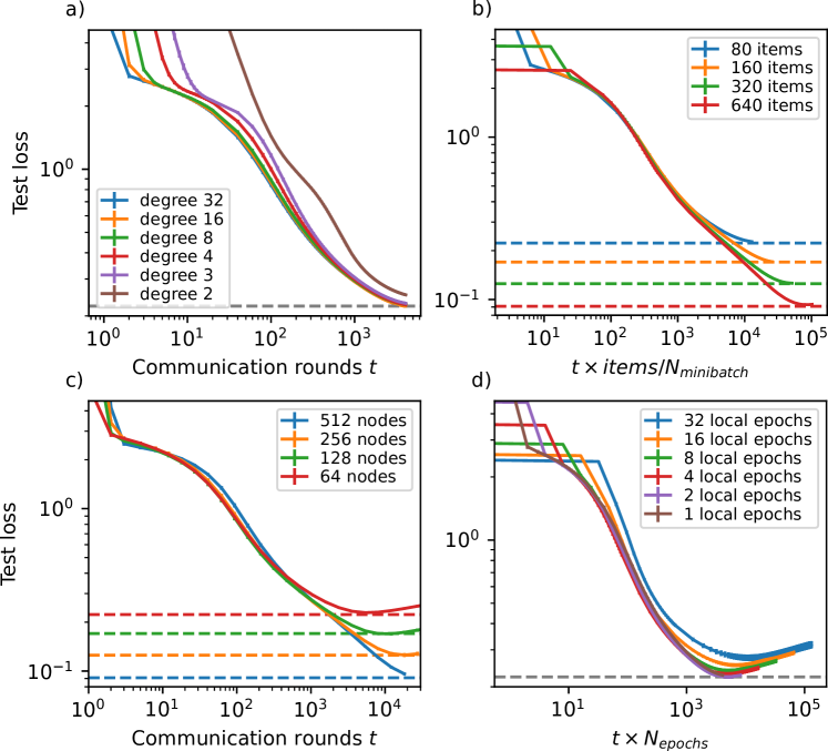
Figure 6: Trajectory of mean test cross-entropy loss over communication rounds for (a) connected random $k$-regular networks with $n=64$ nodes and different values for degree $k$, with 80 balanced training samples per node, (b) 32-regular random network with different number of total labelled training samples, balanced across classes, assigned to each item, (c) with different number of nodes and (d) with different number of local epochs between communications. In all panels, the horizontal dashed lines correspond to the best test loss of a central system with the same amount of the total number of training samples as the entire decentralised federated learning system simulated. Error bars represent 95% confidence intervals. The horizontal axes in (b,d) are scaled to show the “wall-clock equivalent”, a value linearly comparable to the total computation cost of a single node until round $t$.

Network density.

The number of links in the communication network directly increases the communication burden on the nodes. Our results (Figure 6(a) show that while a very small value for the average degree affects the rapidity of the training convergence disproportionately, as long as the average degree is significantly larger than the critical threshold for connectivity, i.e., for random network models with average excess degree $\langle q(k)\rangle\gg 1$, the trajectory will be quite consistent across different network densities. Note that, although in Section 4.2 we were mostly concerned with the scaling of the initial mixing time with the number of nodes, in many cases this would also benefit from a higher average degree. Also note that average degrees close to the critical threshold might not prove practical or desirable for the communication network in the first place, as the network close to the critical threshold is highly susceptible to fragmentation with the cutting off of even very few links.

Training samples per node.

Assuming that each device is capable of performing training on a constant rate of mini-batches per unit of time, more training samples per node increase the total amount of training data, while also linearly increasing the training time for every epoch. Our results (Figure 6(b)) show that (1) the test loss approaches that of a centralised system with the same number of total training samples, and (2) that the trajectory of test loss with effective wall-clock time remains consistent.

System size and total computation cost.

The number of nodes in the network affects the training process in multiple ways. If a larger system size is synonymous with a proportionate increase in the total number of training samples available to the system as a whole, it is interesting to see if the system is capable of utilising those in the same way as an increase in the number of items per node would. Our results (Figure 6(c)) show that if the increase in size coincides with an increase in the total number of items, the system is able to effectively utilise these, always approaching the test loss limit of a centralised system with the same total data.

Another aspect is that an increase in the number of nodes would mean an increase in the total computation cost, so it would be interesting to analyse if this increase (without a corresponding increase in the total amount of data) would result in any improvements in the learning trajectory. In short, our results in Figure 7 show that if the same amount of data is spread across more nodes, each node will have to train on roughly the same number of minibatches to arrive at a similar test loss, and that this result is even consistent with the learning trajectory of the centralised 1 node scenario.

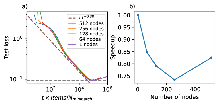
Figure 7: (a) Trajectory of mean test cross-entropy loss over wall-clock time equivalent over 32-regular random graphs and for an isolated node while keeping the total number of training samples across the whole system constant. Each node was assigned training samples balanced across 10 classes, with a total of 40 960 training samples divided equally across the nodes. Error bars represent 95% confidence intervals. The horizontal dashed line corresponds to the best test loss of a central system with the same total amount of training samples as the entire decentralised federated learning system simulated. The sloped dashed line shows the power-law trajectory of loss with equivalent to wall-clock time consistent with results from Henighan et al. (2020). (b) “Slowdown” as a result of splitting the same total amount of training samples across more nodes. Values are calculated as $\tau_{1}(0.11)/\tau_{n}(0.11)$ where $\tau_{n}(l)$ is the wall-clock time equivalent (values of horizontal axis from panel (a)) required for a system with $n$ nodes to reach cross-entropy loss value $l$.

Communication frequency.

Finally, we consider the role of frequency of communication in the trajectory of loss, manifested as the number of local training epochs between communications. It has been shown in the context of decentralised parallel stochastic gradient descent that a higher frequency of communications increases the efficacy of the training process, as it prevents a larger drift (Lian et al., 2017). While a similar phenomenon in the context of an uncoordinated decentralised federated learning seems plausible, showing this relationship empirically on a system of reasonable size was fraught with difficulties due to the issues discussed in Figure 1. Utilising the proposed initialisation method enables this and allows us to confirm (Figure 6(d)) that while more frequent communication increases the communication burden on the entire network, more frequent communication translates to both a lower final test loss as well as faster convergence.

6 Conclusion

Here we introduced a fully uncoordinated, decentralised artificial neural network initialisation method that provides a significantly improved training trajectory on par with coordinated homogeneous initialisation while solely relying on the macroscopic properties of the communication network. We also showed that the initial stages of the uncoordinated decentralised federated learning process are governed by dynamics similar to those of the lazy random walk on graphs. We also discussed preliminary empirical evidence showing that the topology of the communication network might significantly affect the scaling of the training curve, quantified by different exponents for a power-law relationship between test loss and the number of communication rounds for different network models. Furthermore, we also showed empirically that when using the proposed initialisation method, the test loss of the decentralised federated learning system can approach that of a centralised system with the same total number of training samples. We showed the final outcome, in terms of the best test loss achieved, is fairly robust to different values of network density as long as the network is supercritical, and it can benefit from more frequent communication between the nodes.

6.1 Limitations and future works

In this work, we have not considered the non-iid labels or unequal allocation of samples, which is frequently studied in other works on this subject, nor did we consider an unequal allocation of computation power among the nodes to focus solely on the role of the initialisation and the network. These can be, and often In real-world settings, these are often combined or correlated with network properties such as the degree or other centrality measures, which might affect the efficacy of the decentralised federated learning process. Understanding the combination and interactions of these aforementioned properties with network features adds another layer of interdependency and complexity to the problem, which most certainly was not addressable without first studying the simpler case presented here. The prospect of extending this work to these more complex settings is interesting to consider.

The federated learning process presented here also does not support heterogeneous machine learning model architectures between nodes. We expect this to become more and more important with the advances in manufacturing, edge computing and device availability. We also did not consider possible heterogeneities in node-to-node communication patterns, such as burstiness or diurnal pattern, which has been shown to affect the rapidity of other network dynamics like spreading and percolation processes (Karsai et al., 2011; Badie-Modiri et al., 2022a, b).

Our work enables uncoordinated decentralised federated learning that can efficiently train a model using all the data available to all nodes without having the nodes share data directly with a centralised server or with each other. While this enables or streamlines some use cases that were not feasible before, it is important to note that trained machine learning models themselves could be used to extract some information about the training data (Carlini et al., 2021, 2023). It is therefore important to not view federated learning as a panacea for data privacy issues but to view direct data sharing as the weakest link in data privacy.

Impact statement

This paper presents work whose goal is to advance the field of Machine Learning. There are many potential societal consequences of our work, none of which we feel must be specifically highlighted here.

References

- Albert et al. (2000) Albert, R., Jeong, H., and Barabási, A.-L. Error and attack tolerance of complex networks. nature, 406(6794):378–382, 2000. doi: 10.1038/35019019. URL https://doi.org/10.1038/35019019.
- Badie-Modiri et al. (2022a) Badie-Modiri, A., Rizi, A. K., Karsai, M., and Kivelä, M. Directed percolation in random temporal network models with heterogeneities. Physical Review E, 105(5):054313, 2022a. doi: 10.1103/PhysRevE.105.054313. URL https://doi.org/10.1103/PhysRevE.105.054313.
- Badie-Modiri et al. (2022b) Badie-Modiri, A., Rizi, A. K., Karsai, M., and Kivelä, M. Directed percolation in temporal networks. Physical Review Research, 4(2):L022047, 2022b. doi: 10.1103/PhysRevResearch.4.L022047. URL https://doi.org/10.1103/PhysRevResearch.4.L022047.
- Barzdin (1993) Barzdin, Y. M. On the realization of networks in three-dimensional space. Selected Works of AN Kolmogorov: Volume III: Information Theory and the Theory of Algorithms, pp. 194–202, 1993. doi: 10.1007/978-94-017-2973-4˙11. URL https://doi.org/10.1007/978-94-017-2973-4_11.
- Beltrán et al. (2023) Beltrán, E. T. M., Pérez, M. Q., Sánchez, P. M. S., Bernal, S. L., Bovet, G., Pérez, M. G., Pérez, G. M., and Celdrán, A. H. Decentralized federated learning: Fundamentals, state of the art, frameworks, trends, and challenges. IEEE Commun. Surv. Tutorials, 25(4):2983–3013, 2023. doi: 10.1109/COMST.2023.3315746. URL https://doi.org/10.1109/COMST.2023.3315746.
- Benjamini et al. (2014) Benjamini, I., Kozma, G., and Wormald, N. The mixing time of the giant component of a random graph. Random Structures & Algorithms, 45(3):383–407, 2014. doi: 10.1002/rsa.20539. URL https://doi.org/10.1002/rsa.20539.
- Carlini et al. (2021) Carlini, N., Tramer, F., Wallace, E., Jagielski, M., Herbert-Voss, A., Lee, K., Roberts, A., Brown, T., Song, D., Erlingsson, U., et al. Extracting training data from large language models. In 30th USENIX Security Symposium (USENIX Security 21), pp. 2633–2650, 2021. URL https://www.usenix.org/conference/usenixsecurity21/presentation/carlini-extracting.
- Carlini et al. (2023) Carlini, N., Hayes, J., Nasr, M., Jagielski, M., Sehwag, V., Tramer, F., Balle, B., Ippolito, D., and Wallace, E. Extracting training data from diffusion models. In 32nd USENIX Security Symposium (USENIX Security 23), pp. 5253–5270, 2023. URL https://www.usenix.org/conference/usenixsecurity23/presentation/carlini.
- Fortunato & Hric (2016) Fortunato, S. and Hric, D. Community detection in networks: A user guide. Physics reports, 659:1–44, 2016. doi: 10.1016/j.physrep.2016.09.002. URL https://doi.org/10.1016/j.physrep.2016.09.002.
- Fountoulakis & Reed (2008) Fountoulakis, N. and Reed, B. A. The evolution of the mixing rate of a simple random walk on the giant component of a random graph. Random Structures & Algorithms, 33(1):68–86, 2008. doi: 10.1002/rsa.20210. URL https://doi.org/10.1002/rsa.20210.
- Gauvin et al. (2022) Gauvin, L., Génois, M., Karsai, M., Kivelä, M., Takaguchi, T., Valdano, E., and Vestergaard, C. L. Randomized reference models for temporal networks. SIAM Review, 64(4):763–830, 2022. doi: 10.1137/19M1242252. URL https://doi.org/10.1137/19M1242252.
- Glorot & Bengio (2010) Glorot, X. and Bengio, Y. Understanding the difficulty of training deep feedforward neural networks. In Proceedings of the thirteenth international conference on artificial intelligence and statistics, pp. 249–256. JMLR Workshop and Conference Proceedings, 2010. URL https://proceedings.mlr.press/v9/glorot10a.html.
- Goodfellow et al. (2016) Goodfellow, I., Bengio, Y., and Courville, A. Deep learning. MIT press, 2016. doi: 10.1038/nature14539. URL https://doi.org/10.1038/nature14539.
- He et al. (2015) He, K., Zhang, X., Ren, S., and Sun, J. Delving deep into rectifiers: Surpassing human-level performance on imagenet classification. In Proceedings of the IEEE international conference on computer vision, pp. 1026–1034, 2015. doi: 10.1109/ICCV.2015.123. URL https://doi.org/10.1109/ICCV.2015.123.
- He et al. (2016) He, K., Zhang, X., Ren, S., and Sun, J. Deep residual learning for image recognition. In Proceedings of the IEEE conference on computer vision and pattern recognition, pp. 770–778, 2016. doi: 10.1109/CVPR.2016.90. URL https://doi.org/10.1109/CVPR.2016.90.
- Henighan et al. (2020) Henighan, T., Kaplan, J., Katz, M., Chen, M., Hesse, C., Jackson, J., Jun, H., Brown, T. B., Dhariwal, P., Gray, S., et al. Scaling laws for autoregressive generative modeling. arXiv preprint 2010.14701, 2020. URL https://arxiv.org/abs/2010.14701.
- Jennings (1937) Jennings, H. Structure of leadership-development and sphere of influence. Sociometry, 1(1/2):99–143, 1937. doi: 0.2307/2785262. URL https://doi.org/0.2307/2785262.
- Kairouz et al. (2021) Kairouz, P., McMahan, H. B., Avent, B., Bellet, A., Bennis, M., Bhagoji, A. N., Bonawitz, K., Charles, Z., Cormode, G., Cummings, R., et al. Advances and open problems in federated learning. Foundations and Trends® in Machine Learning, 14(1–2):1–210, 2021. doi: 10.1561/2200000083. URL https://doi.org/10.1561/2200000083.
- Karsai et al. (2011) Karsai, M., Kivelä, M., Pan, R. K., Kaski, K., Kertész, J., Barabási, A.-L., and Saramäki, J. Small but slow world: How network topology and burstiness slow down spreading. Physical Review E, 83(2):025102, 2011. doi: 10.1103/PhysRevE.83.025102. URL https://doi.org/10.1103/PhysRevE.83.025102.
- Lalitha et al. (2018) Lalitha, A., Shekhar, S., Javidi, T., and Koushanfar, F. Fully decentralized federated learning. In Third workshop on bayesian deep learning (NeurIPS), volume 2, 2018. URL http://bayesiandeeplearning.org/2018/papers/140.pdf.
- LeCun et al. (1998) LeCun, Y., Bottou, L., Bengio, Y., and Haffner, P. Gradient-based learning applied to document recognition. Proceedings of the IEEE, 86(11):2278–2324, 1998. doi: 10.1109/5.726791. URL https://doi.org/10.1109/5.726791.
- LeCun et al. (2002) LeCun, Y., Bottou, L., Orr, G. B., and Müller, K.-R. Efficient backprop. In Neural networks: Tricks of the trade, pp. 9–50. Springer, 2002. doi: 10.1007/978-3-642-35289-8˙3. URL https://doi.org/10.1007/978-3-642-35289-8_3.
- Levin & Peres (2017) Levin, D. A. and Peres, Y. Markov chains and mixing times, volume 107. American Mathematical Soc., 2017.
- Lian et al. (2017) Lian, X., Zhang, C., Zhang, H., Hsieh, C.-J., Zhang, W., and Liu, J. Can decentralized algorithms outperform centralized algorithms? a case study for decentralized parallel stochastic gradient descent. In Advances in Neural Information Processing Systems, volume 30, 2017. URL https://proceedings.neurips.cc/paper_files/paper/2017/file/f75526659f31040afeb61cb7133e4e6d-Paper.pdf.
- Luce & Perry (1949) Luce, R. D. and Perry, A. D. A method of matrix analysis of group structure. Psychometrika, 14(2):95–116, 1949. doi: 10.1007/BF02289146. URL https://doi.org/10.1007/BF02289146.
- McMahan et al. (2017) McMahan, B., Moore, E., Ramage, D., Hampson, S., and y Arcas, B. A. Communication-efficient learning of deep networks from decentralized data. In Artificial intelligence and statistics, pp. 1273–1282. PMLR, 2017. URL http://proceedings.mlr.press/v54/mcmahan17a.html.
- Newman (2010) Newman, M. E. J. Networks: An introduction. Oxford UP, 2010. doi: 10.1093/acprof:oso/9780199206650.001.0001.
- Nguyen et al. (2022) Nguyen, J., Malik, K., Sanjabi, M., and Rabbat, M. Where to begin? exploring the impact of pre-training and initialization in federated learning. arXiv preprint 2206.15387, 2022. URL https://arxiv.org/abs/2206.15387.
- Orsini et al. (2015) Orsini, C., Dankulov, M. M., Colomer-de Simón, P., Jamakovic, A., Mahadevan, P., Vahdat, A., Bassler, K. E., Toroczkai, Z., Boguná, M., Caldarelli, G., et al. Quantifying randomness in real networks. Nature communications, 6(1):8627, 2015. doi: 10.1038/ncomms9627. URL https://doi.org/10.1038/ncomms9627.
- Palmieri et al. (2023) Palmieri, L., Valerio, L., Boldrini, C., and Passarella, A. The effect of network topologies on fully decentralized learning: a preliminary investigation. In Proceedings of the 1st International Workshop on Networked AI Systems, pp. 1–6, 2023. doi: 10.1145/3597062.3597280. URL https://doi.org/10.1145/3597062.3597280.
- Peres & Sousi (2015) Peres, Y. and Sousi, P. Mixing times are hitting times of large sets. Journal of Theoretical Probability, 28(2):488–519, 2015. doi: 10.1007/s10959-013-0497-9. URL https://doi.org/10.1007/s10959-013-0497-9.
- Pinsker (1973) Pinsker, M. S. On the complexity of a concentrator. In 7th International Telegraffic Conference, volume 4, pp. 1–318. Citeseer, 1973. URL https://citeseerx.ist.psu.edu/document?repid=rep1&type=pdf&doi=71c9fd11ff75889aaa903b027af3a06e750e8add.
- Qu et al. (2020) Qu, Y., Pokhrel, S. R., Garg, S., Gao, L., and Xiang, Y. A blockchained federated learning framework for cognitive computing in industry 4.0 networks. IEEE Transactions on Industrial Informatics, 17(4):2964–2973, 2020. doi: 10.1109/TII.2020.3007817. URL https://doi.org/10.1109/TII.2020.3007817.
- Rice (1927) Rice, S. A. The identification of blocs in small political bodies. American Political Science Review, 21(3):619–627, 1927. doi: 10.2307/1945514. URL https://doi.org/10.2307/1945514.
- Rieke et al. (2020) Rieke, N., Hancox, J., Li, W., Milletari, F., Roth, H. R., Albarqouni, S., Bakas, S., Galtier, M. N., Landman, B. A., Maier-Hein, K., et al. The future of digital health with federated learning. NPJ digital medicine, 3(1):119, 2020. doi: 10.1038/S41746-020-00323-1. URL https://doi.org/10.1038/S41746-020-00323-1.
- Roy et al. (2019) Roy, A. G., Siddiqui, S., Pölsterl, S., Navab, N., and Wachinger, C. Braintorrent: A peer-to-peer environment for decentralized federated learning. arXiv preprint 1905.06731, 2019. URL https://arxiv.org/abs/1905.06731.
- Savazzi et al. (2021) Savazzi, S., Nicoli, M., Bennis, M., Kianoush, S., and Barbieri, L. Opportunities of federated learning in connected, cooperative, and automated industrial systems. IEEE Communications Magazine, 59(2):16–21, 2021. doi: 10.1109/MCOM.001.2000200. URL https://doi.org/10.1109/10.1109/MCOM.001.2000200.
- Sun et al. (2022) Sun, T., Li, D., and Wang, B. Decentralized federated averaging. IEEE Transactions on Pattern Analysis and Machine Intelligence, 45(4):4289–4301, 2022. doi: 10.1109/TPAMI.2022.3196503. URL https://doi.org/10.1109/TPAMI.2022.3196503.
- Tedeschini et al. (2022) Tedeschini, B. C., Savazzi, S., Stoklasa, R., Barbieri, L., Stathopoulos, I., Nicoli, M., and Serio, L. Decentralized federated learning for healthcare networks: A case study on tumor segmentation. IEEE Access, 10:8693–8708, 2022. doi: 10.1109/ACCESS.2022.3141913. URL https://doi.org/10.1109/ACCESS.2022.3141913.
- Valerio et al. (2023) Valerio, L., Boldrini, C., Passarella, A., Kertész, J., Karsai, M., and Iñiguez, G. Coordination-free decentralised federated learning on complex networks: Overcoming heterogeneity. arXiv preprint 2312.04504, 2023. URL https://arxiv.org/abs/2312.04504.
- Vogels et al. (2022) Vogels, T., Hendrikx, H., and Jaggi, M. Beyond spectral gap: The role of the topology in decentralized learning. In Advances in Neural Information Processing Systems, volume 35, pp. 15039–15050, 2022. URL https://proceedings.neurips.cc/paper_files/paper/2022/file/61162d94822d468ee6e92803340f2040-Paper-Conference.pdf.
- Watts & Strogatz (1998) Watts, D. J. and Strogatz, S. H. Collective dynamics of ‘small-world’ networks. nature, 393(6684):440–442, 1998. doi: 10.1038/30918. URL https://doi.org/10.1038/30918.