On the Stability of Learning
in Network Games with Many Players

Abstract.

Multi-agent learning algorithms have been shown to display complex, unstable behaviours in a wide array of games. In fact, previous works indicate that convergent behaviours are less likely to occur as the total number of agents increases. This seemingly prohibits convergence to stable strategies, such as Nash Equilibria, in games with many players.

To make progress towards addressing this challenge we study the Q-Learning Dynamics, a classical model for exploration and exploitation in multi-agent learning. In particular, we study the behaviour of Q-Learning on games where interactions between agents are constrained by a network. We determine a number of sufficient conditions, depending on the game and network structure, which guarantee that agent strategies converge to a unique stable strategy, called the Quantal Response Equilibrium (QRE). Crucially, these sufficient conditions are independent of the total number of agents, allowing for provable convergence in arbitrarily large games.

Next, we compare the learned QRE to the underlying NE of the game, by showing that any QRE is an $\epsilon$-approximate Nash Equilibrium. We first provide tight bounds on $\epsilon$ and show how these bounds lead naturally to a centralised scheme for choosing exploration rates, which enables independent learners to learn stable approximate Nash Equilibrium strategies. We validate the method through experiments and demonstrate its effectiveness even in the presence of numerous agents and actions. Through these results, we show that independent learning dynamics may converge to approximate Nash Equilibria, even in the presence of many agents.

1. Introduction

Game Theory (EGT) has emerged as a powerful formalism for studying learning in multi-agent settings Schwartz (2014); Tuyls (2023). Here, agents are required to explore their state space to determine optimal actions, whilst simultaneously maximising their expected reward in the face of the changing behaviour of their opponents. By modelling these situations as idealised games it is possible to study the effect of various factors, such as payoffs and number of agents, on the dynamics of learning. An important question which is often studied from this lens is whether popular multi-agent learning algorithms converge to an equilibrium Metrick and Polak (1994); Harris (1998); Leonardos and Piliouras (2022) (most often the Nash Equilibrium).

Unfortunately, it seems that the general answer to this question is no. Recent work has shown that, even in zero-sum games, the dynamics of no-regret learning algorithms can be cyclic Mertikopoulos et al. (2018) or chaotic Cheung and Piliouras (2019). In addition, even small deviations from the zero-sum setting can result in robustly non-convergent dynamics Cheung and Tao (2020); Hussain et al. (2023a) so that in general-sum games, non-convergent behaviour appears to be the norm Pangallo et al. (2019, 2022); Galla and Farmer (2013); Vlatakis-Gkaragkounis et al. (2020); Kleinberg et al. (2011); Imhof et al. (2005); Galla (2011); van Strien and Sparrow (2011); Sato et al. (2004); Griffin et al. (2022). To make matters worse, recent findings in Sanders et al. (2018) suggest that, as the number of agents in the game increases, the likelihood for chaotic dynamics also increases when agents have low exploration rates. Similarly, the results of Hussain et al. (2023b) imply that incredibly large exploration rates may be required in games with many agents in order to ensure convergence. This seemingly presents a bottleneck for strong convergence guarantees in multi-agent settings with many agents.

Despite this, many real world problems such as resource allocation Amelina et al. (2015); Parise et al. (2020), routing Bielawski et al. (2021); Chotibut et al. (2019a, b) and robotics Hamann (2018); Shokri and Kebriaei (2020) consider a large number of agents who continuously adapt to one another. These practical applications in conjunction with the negative results in the face of many players immediately yield the following question:

Is there any hope for independent learning agents to converge to an equilibrium in games with many players?

To make progress in answering this question, this work examines multi-agent learning in network games. Here, it is assumed that agents can only interact with their neighbours within an underlying communication network. Such systems are ubiquitous: machine learning architectures often impose structure between models Hoang et al. (2018); LI et al. (2017); in robotic systems, agents interact through communication networks Grammatico et al. (2016); Shokri and Kebriaei (2020); in both economics and biology, agent interactions are constrained through social networks. Network games refine the setting of Sanders et al. (2018); Hussain et al. (2023b), in which it was assumed that each agent is directly influenced by every other agent in the environment. This work provides strong evidence that the network structure matters, in some cases even more so than the total number of agents.

Model and Contribution

We consider agents who update via the Q-Learning dynamic, Sato and Crutchfield (2003); Tuyls et al. (2006), a foundational model from game theory which describes the behaviour of agents who balance exploration and exploitation. Similar to Hussain et al. (2023b) we determine a number of sufficient conditions on exploration rates such that Q-Learning is guaranteed to converge to a unique equilibrium. In this work, however, we find that these conditions depend on graph theoretic properties of the interaction network. In our experiments, we examine how these conditions depend on the total number of agents and find network structures for which there is no explicit dependence. These implications are visualised on a number of representative network games and it is shown that large numbers of agents may converge to an equilibrium, so long as weakly connected network structures are used. By contrast, if the network is strongly connected, we recover the results of Hussain et al. (2023b); Sanders et al. (2018) and show that stability depends on the total number of agents.

The equilibrium solution to which Q-Learning converges is the Quantal Response Equilibrium (QRE) McKelvey and Palfrey (1995); Leonardos et al. (2021), a widely studied extension of the Nash Equilibrium for agents who explore their state space Leonardos and Piliouras (2022); Kianercy and Galstyan (2012); Gemp et al. (2022). In this work, we quantify the ‘distance’ between a QRE and NE by showing that any QRE is an approximate Nash Equilibrium and providing tight bounds on this approximation. Using this, we present a procedure for choosing exploration rates so that Q-Learning agents may converge ‘closer’ to the Nash Equilibrium, whilst maintaining the stability of the dynamic. We validate this procedure in a number of large scale network games and show that it leads to improvements in the convergence of Q-Learning dynamics towards approximate Nash Equilibria.

Related Work

In Galla and Farmer (2013) the authors showed that the Experience Weighted Attraction (EWA) dynamic, which is closely related to Q-Learning (Leonardos et al., 2021), achieves chaos in classes of two-player games. Advancing this result, Sanders et al. (2018) showed that chaotic dynamics become more prevalent as the number of agents increase. Similar to this work, Hussain et al. (2023b) apply the framework of monotone game Parise and Ozdaglar (2019); Facchinei and Pang (2004); Tatarenko and Kamgarpour (2019) to show that Q-Learning Dynamics converge to a unique equilibrium in any game, given sufficient exploration. However, they also find that this condition increases with the number of agents.

Besides online learning, other approaches have been developed to try to compute Nash Equilibria in games. For our purposes, the most relevant of these are homotopy-like methods Turocy (2005); Herings and Peeters (2010). The principle of these methods is to perturb the payoff functions so that the resulting perturbed game is ‘easier’ to solve. Then, by iteratively annealing this perturbation, one can approximate the underlying NE. Recently Gemp et al. (2022) applies an entropy perturbation of payoffs and use gradient-descent based approach to solve for a continuum of Quantal Response Equilibria (QRE), which eventually leads to a NE McKelvey and Palfrey (1995). Whilst homotopy methods present a powerful tool for computing approximate equilibria, they often lack the advantages of decentralisation provided by online learning and may not come with strong guarantees. Perolat et al. (2020) combines the entropy perturbation approach with online learning and show that, in two-player zero-sum games, this method allows independent learners to converge asymptotically to an NE. However, as with most learning strategies, its behaviour in many player, general sum games is unknown.

We address the problem of learning in many player games by examining the role of an underlying communication network. A number of works in game theory have shown that network structure affects the uniqueness and stability of NE Ballester et al. (2006); Bramoullé et al. (2014); Parise and Ozdaglar (2019); Melo (2018); Czechowski and Piliouras (2022). Our main result refines that of Hussain et al. (2023b) to include the network and show that Q-Learning dynamics can reach a QRE in any network game, given sufficiently high exploration rates. Crucially, these conditions are explicitly independent of the total number of agents. We also show that the QRE achieved by Q-Learning is an approximate Nash Equilibrium, and design a centralised scheme for updating exploration rates so that Q-Learning dynamics converge along the continuum of stable QRE to an approximate Nash Equilibrium.

2. Preliminaries

We begin in Section 2.1 by defining the network game model, which is the setting on which we study the Q-Learning dynamics, which we describe in Section 2.2.

2.1. Game Model

In this work, we consider network polymatrix games Leonardos et al. (2021). A Network Game is described by the tuple $\mathcal{G}=(\mathcal{N},\mathcal{E},(u_{k},\mathcal{S}_{k})_{k\in\mathcal{N}})$, where $\mathcal{N}$ denotes a finite set $\mathcal{N}$ of players, indexed by $k=1,\ldots,N$. Each agent can choose from a finite set $\mathcal{S}_{k}$ of actions, indexed by $i=1,\ldots,n$. We denote the strategy $\mathbf{x}_{k}$ of an agent $k$ as the probabilities with which they play their actions. Then, the set of all strategies of agent $k$ is $\Delta(\mathcal{S}_{k}):=\left\{\mathbf{x}_{k}\in\mathbb{R}^{n}\,:\,\sum_{i}x_{ki}=1,x_{ki}\geq 0\right\}$. Each agent is also given a payoff function $u_{k}\,:\Delta(\mathcal{S}_{k})\times\Delta(\mathcal{S}_{-k})\rightarrow\mathbb{R}$. Agents are connected via an underlying network defined by $\mathcal{E}$. In particular, $\mathcal{E}$ consists of pairs $(k,l)\in\mathcal{N}\times\mathcal{N}$ of connected agents $k$ and $l$. For any agent $k\in\mathcal{N}$, we denote by $\mathcal{N}_{k}=\{l\in\mathcal{N}:(k,l)\in\mathcal{E}\}$ the neighbours of $k$, i.e. all the agents who directly interact with agent $k$ in the network. An equivalent way to define the network is through an adjacency matrix $G$ such that

$$[G]_{k,l}=\begin{cases}1,\text{ if agents $k,l$ are connected,}\\ 0,\text{ otherwise.}\end{cases}.$$

It is assumed that the network is undirected so that $G$ is a symmetric matrix. Each edge $(k,l)\in\mathcal{E}$ corresponds to a pair of payoff matrices $A^{kl}$, $A^{lk}$. With these specifications, the payoff received by each agent $k$ under joint strategy $\mathbf{x}=(\mathbf{x}_{k},\mathbf{x}_{-k})$ is given by

$$u_{k}(\mathbf{x}_{k},\mathbf{x}_{-k})=\sum_{(k,l)\in\mathcal{E}}\mathbf{x}_{k}\cdot A^{kl}\mathbf{x}_{l}.$$ (1)

For any $\mathbf{x}\in\Delta=:\times_{k}\Delta(\mathcal{S}_{k})$, we can define the reward to agent $k$ for playing action $i$ as $r_{ki}(\mathbf{x}_{-k})=\partial u_{ki}(\mathbf{x})/\partial x_{ki}$. Under this notation, $u_{k}(\mathbf{x}_{k},\mathbf{x}_{-k})=\langle\mathbf{x}_{k},r_{k}(\mathbf{x}_{-k})\rangle$. With this in place, we can define suitable equilibrium solutions for the game.

Definition 2.1 (Nash Equilibrium (NE)).

A joint mixed strategy $\mathbf{\bar{x}}\in\Delta$ is a Nash Equilibrium (NE) if, for all agents $k$ and all actions $i\in\mathcal{S}_{k}$

$$\mathbf{\bar{x}}_{k}=\arg\max_{\mathbf{y}_{k}\in\Delta_{k}}u_{k}(\mathbf{y}_{k},\mathbf{\bar{x}}_{-k}).$$

Definition 2.2 (Quantal Response Equilibrium (QRE)).

A joint mixed strategy $\mathbf{\bar{x}}\in\Delta$ is a Quantal Response Equilibrium (QRE) if, for all agents $k$ and all actions $i\in\mathcal{S}_{k}$

$$\mathbf{\bar{x}}_{ki}=\frac{\exp(r_{ki}(\mathbf{\bar{x}}_{-k})/T_{k})}{\sum_{j\in\mathcal{S}_{k}}\exp(r_{kj}(\mathbf{\bar{x}}_{-k})/T_{k})}.$$

The QRE Camerer et al. (2004); McKelvey and Palfrey (1995) naturally extends the Nash Equilibrium through the parameter $T_{k}$, known as the exploration rate. In particular, the limit $T_{k}\rightarrow 0$ corresponds exactly to the Nash Equilibrium, whereas the limit $T_{k}\rightarrow\infty$ corresponds to the case where action $i\in\mathcal{S}_{k}$ is played with the same probability regardless of its associated reward. The link between the QRE and the Nash Equilibrium is made precise through the following result.

Proposition 2.3 (Melo (2021)).

Consider a game $\mathcal{G}=(\mathcal{N},\mathcal{E},(u_{k},\mathcal{S}_{k})_{k\in\mathcal{N}})$ and let $T_{1},\ldots,T_{N}>0$ be exploration rates. Define the perturbed game $\mathcal{G}^{H}=(\mathcal{N},\mathcal{E},(u_{k}^{H},\mathcal{S}_{k})_{k\in\mathcal{N}})$ with the payoff functions

$$u_{k}^{H}(\mathbf{x}_{k},\mathbf{x}_{-k})=u_{k}(\mathbf{x}_{k},\mathbf{x}_{-k})-T_{k}\langle\mathbf{x}_{k},\ln\mathbf{x}_{k}\rangle.$$

Then $\mathbf{\bar{x}}\in\Delta$ is a QRE of $\mathcal{G}$ iff it is a Nash Equilibrium of $\mathcal{G}^{H}$.

Game Structure

To achieve our main result, we must parameterise interactions in the network game. This allows us to consider network games which are not necessarily zero-sum. First, we define the influence bound for each agent $k$.

Definition 2.4 (Influence Bound).

Let $\mathcal{G}=(\mathcal{N},\mathcal{E},(u_{k},\mathcal{S}_{k})_{k\in\mathcal{N}})$ be a network game. Then, for any $k\in\mathcal{N}$, the influence bound is given by

$$\delta_{k}=\max_{i\in\mathcal{S}_{k},a_{-k},\tilde{a}_{-k}\in\mathcal{S}_{-k}}\{|r_{ki}(a_{-k})-r_{ki}(\tilde{a}_{-k})|\},$$ (2)

where the pure strategies $a_{-k},\tilde{a}_{-k}\in\mathcal{S}_{-k}$ differ only in the action of one agent $l\in\mathcal{N}_{k}$.

The influence bound describes how sensitive each agent’s reward is to changes in opponent strategies. As another parameterisation which is directly applicable to network games, we define the intensity of identical interests.

Definition 2.5 (Intensity of Identical Interests).

Let $\mathcal{G}$ be a network game whose edgeset $\mathcal{E}$ is associated with the payoff matrices $(A^{kl},A^{lk})_{(k,l)\in\mathcal{E}}$. The intensity of identical interests $\sigma_{I}$ of $\mathcal{G}$ is given as

$$\sigma_{I}=\max_{(k,l)\in\mathcal{E}}\lVert A^{kl}+(A^{lk})^{\top}\rVert_{2},$$ (3)

where $\lVert M\rVert_{2}=\sup_{\|\mathbf{x}\rVert_{2}=1}\lVert M\mathbf{x}\rVert_{2}$ denotes the operator $2$-norm Meiss (2007).

The intensity of identical interests can be thought of as a measure of how cooperative a network game is. The reasoning for this is as follows. Suppose $A,B$ are the payoff matrices which maximise (3) and suppose that $B^{\top}=cA$ for some $c=(-1,1)$. Then, $\sigma_{I}$ is minimised when $c=-1$, in which case $A,B$ is zero-sum, and is maximised at $c=1$ so that $A=B^{\top}$, which defines an game of identical interests.

2.2. Learning Model

In this work, we analyse the Q-Learning dynamic, a prototypical model for determining optimal policies by balancing exploration and exploitation Sutton and Barto (2018); Schwartz (2014). In this model, each agent $k\in\mathcal{N}$ maintains a history of the past performance of each of their actions. This history is updated via the Q-update

$$Q_{ki}(\tau+1)=(1-\alpha_{k})Q_{ki}(\tau)+\alpha_{k}r_{ki}(\mathbf{x}_{-k}(\tau)),$$

where $\tau$ denotes the current time step.

$Q_{ki}(\tau)$ denotes the Q-value maintained by agent $k$ about the performance of action $i\in S_{k}$. In effect, $Q_{ki}$ gives a discounted history of the rewards received when $i$ is played, with $1-\alpha_{k}$ as the discount factor.

Given these Q-values, each agent updates their mixed strategies according to the Boltzmann distribution, given by

$$x_{ki}(\tau)=\frac{\exp(Q_{ki}(\tau)/T_{k})}{\sum_{j}\exp(Q_{kj}(\tau)/T_{k})},$$

in which $T_{k}\in[0,\infty)$ is the exploration rate of agent $k$.

It was shown in Tuyls et al. (2006); Sato and Crutchfield (2003) that a continuous time approximation of the Q-Learning algorithm could be written as

$$\frac{\dot{x}_{ki}}{x_{ki}}=r_{ki}\left(\mathbf{x}_{-k}\right)-\langle\mathbf{x}_{k},r_{k}(\mathbf{x})\rangle+T_{k}\sum_{j\in S_{k}}x_{kj}\ln\frac{x_{kj}}{x_{ki}},$$ (QLD)

which we call the Q-Learning dynamics (QLD). The fixed points of this dynamic coincide with the (QRE) of the game Leonardos et al. (2021). QLD can also be seen as an entropy regularised form of the well-studied replicator dynamics (RD) Maynard Smith (1974); Hofbauer and Sigmund (1998). Besides its importance in the study of population biology Mukhopadhyay and Chakraborty (2020), RD is known to be a special case of the generalised Follow the Regularised Leader learning dynamic Mertikopoulos and Sandholm (2016), which models agents who maximise their accumulated payoffs subject to a penalisation function. RD has been shown to display asymptotic convergence in potential games Hofbauer and Sigmund (1998), cyclic behaviour in zero-sum games Mertikopoulos et al. (2018) and chaos in a number of other classes Sato et al. (2002); Griffin et al. (2022). The connection between RD and QLD is explored in Leonardos and Piliouras (2022).

3. Guaranteed Convergence of Q-Learning in Network Games

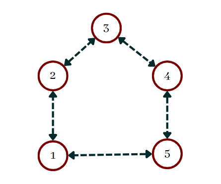
Ring Network
$\left\lVert G\right\rVert_{\infty}=2,\left\lVert G\right\rVert_{2}=2$

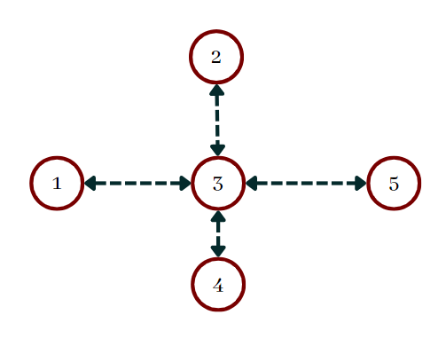
Star Network
$\left\lVert G\right\rVert_{\infty}=N-1,\left\lVert G\right\rVert_{2}=\sqrt{N-1}$

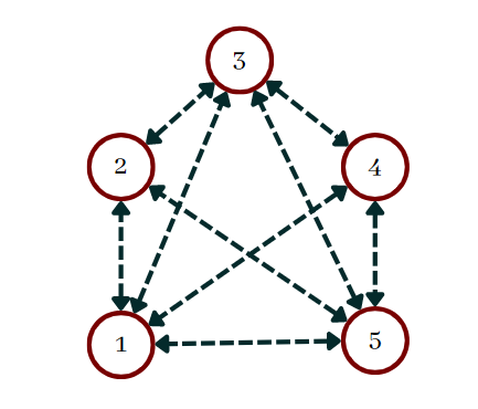
Fully Connected Network
$\left\lVert G\right\rVert_{\infty}=N-1,\left\lVert G\right\rVert_{2}=N-1$

Figure 1. Examples of networks with five agents and associated $\left\lVert G\right\rVert_{\infty}$ and $\left\lVert G\right\rVert_{2}$.

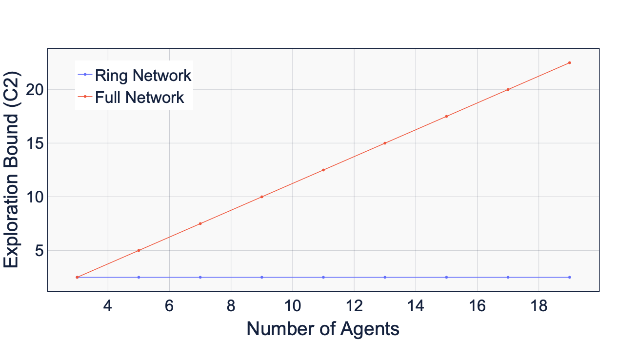
Shapley Game

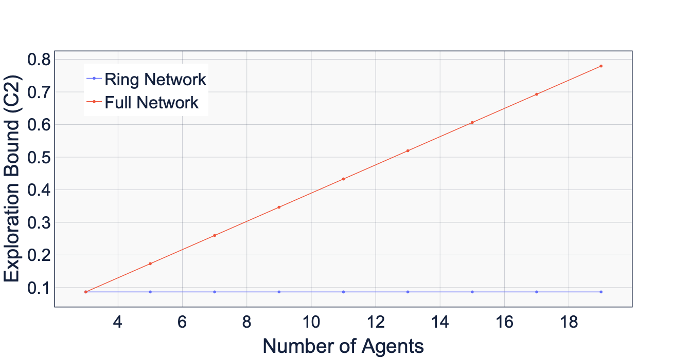
Sato Game

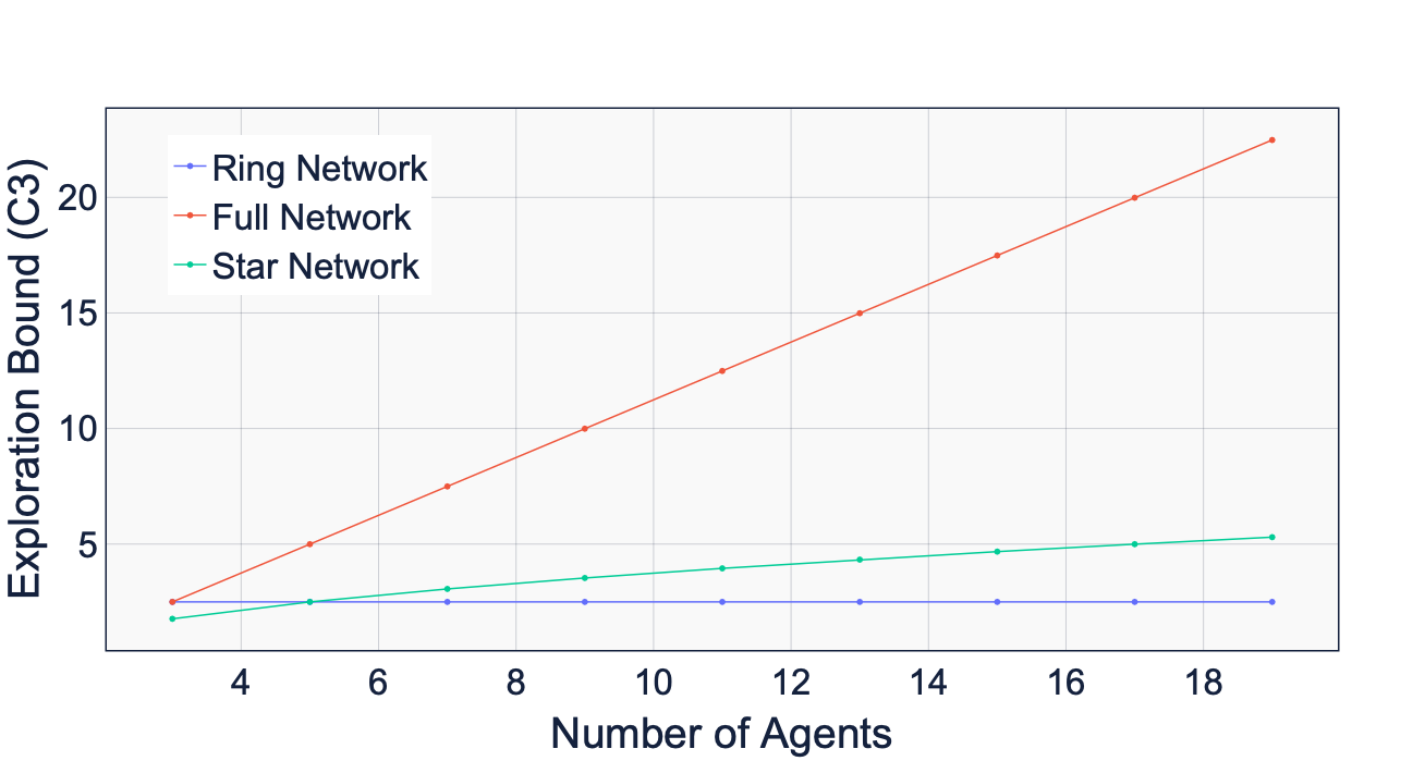
Shapley Game

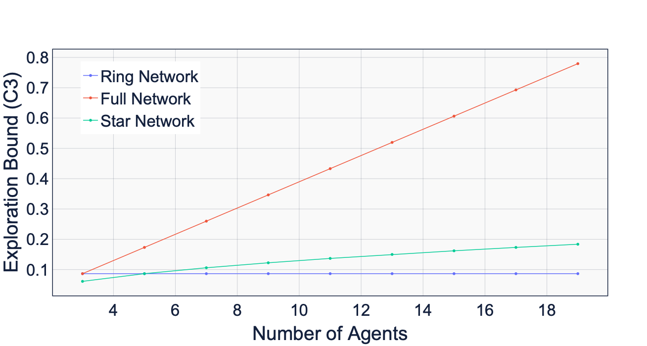
Sato Game

Figure 2. Lower Bound on sufficient exploration as defined by (Top) (C2) in a Full Network and Ring Network (Bottom) (C3) in a Full Network, Star Network and Full Network.

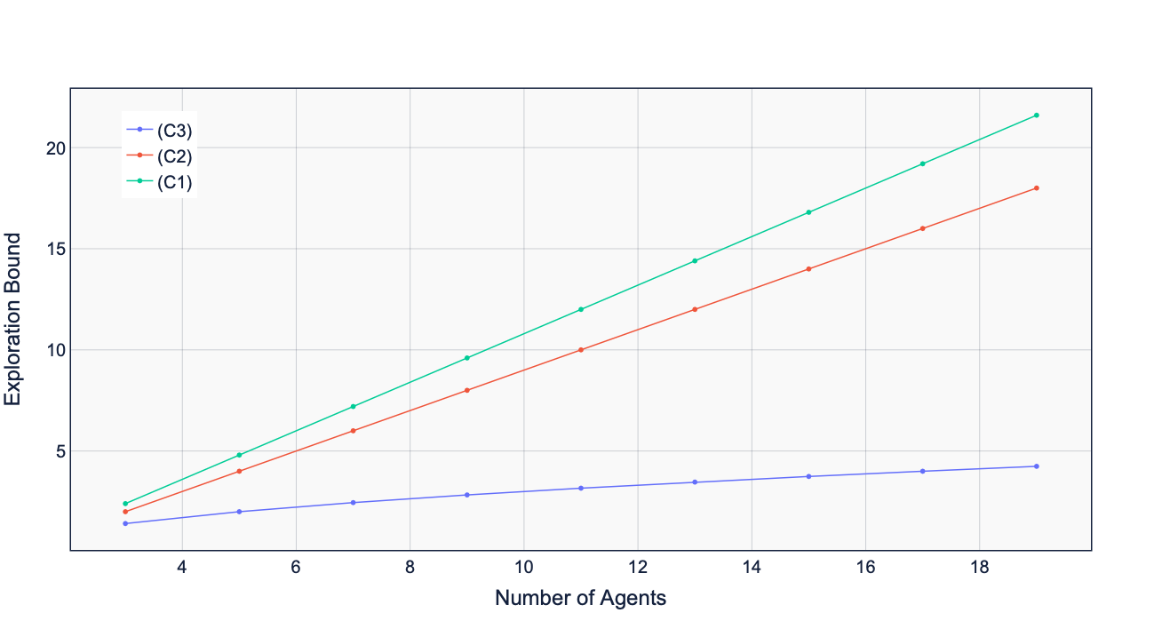
Shapley Game

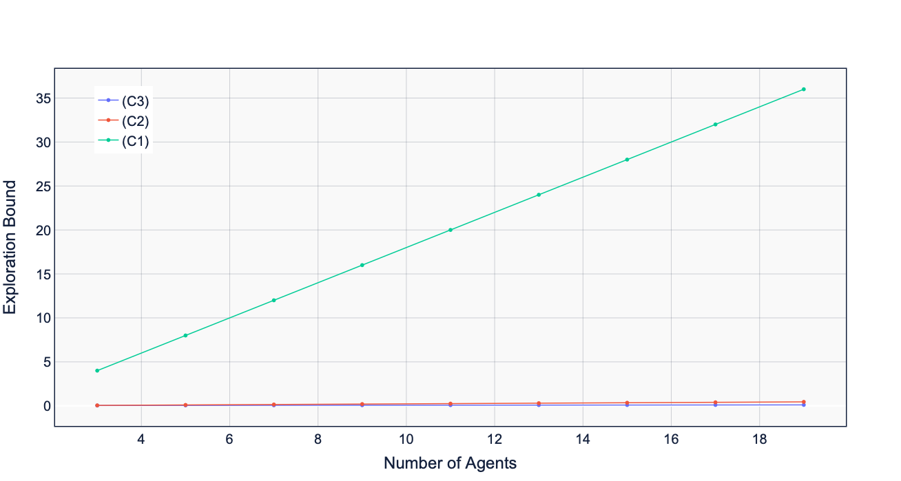
Sato Game

Figure 3. Lower Bound on sufficient exploration as defined by (C1), (C2) and (C3) in a Star Network. For (C1), $\max_{k\in\mathcal{N}}\delta_{k}|\mathcal{N}_{k}|$ is depicted which therefore coincides with the condition defined in Hussain et al. (2023b).

In this section we determine a number of sufficient conditions on the exploration rates $T_{k}$ under which Q-Learning dynamics converge to a unique QRE. We find that these conditions are dependent on the structure of the rewards in the game, parameterised by the interaction coefficient or the inflence bound, and also on the structure of the network. We then compare our result to that of Hussain et al. (2023b) and show that, under suitable network structures, stability can be achieved with comparatively low exploration rates, even in the presence of many players. This also refines the result of Sanders et al. (2018) which suggests that learning dynamics are increasingly unstable as the number of players increases, regardless of exploration rate. All proofs are in Appendix B.

Theorem 3.1.

Consider a network game $\mathcal{G}=(\mathcal{N},\mathcal{E},(u_{k},\mathcal{S}_{k})_{k\in\mathcal{N}})$ which has a network adjacency matrix $G$. Let $\sigma_{I}$ denote the intensity of identical interests for $\mathcal{G}$ and $\delta_{k}$ denote the influence bound of each agent $k\in\mathcal{N}$. Then, the Q-Learning Dynamic converges to a unique QRE $\mathbf{\bar{x}}\in\Delta$ if any of the following conditions hold for all agents $k\in\mathcal{N}$,

$$T_{k} >\delta_{k}|\mathcal{N}_{k}|,$$ (C1)

$$T_{k} >\frac{1}{2}\sigma_{I}\left\lVert G\right\rVert_{\infty},$$ (C2)

where $\lVert M\rVert_{\infty}=\max_{i}\sum_{j}|[M]_{ij}|$ is the operator $\infty$-norm. If, in addition, each edge defines the same bimatrix game $(A,B)$, then asymptotic convergence of Q-Learning Dynamics holds if, for all $k\in\mathcal{N}$

$$T_{k}>\frac{1}{2}\sigma_{I}\left\lVert G\right\rVert_{2}.$$ (C3)

Remark 3.2.

Condition (C1) immediately refines the result of Hussain et al. (2023b) to the case of network games. In the latter work, the authors implicitly assume that the reward for each agent depends on all other agents. In our work, this corresponds exactly to the case of a fully connected network, where $\mathcal{N}_{k}=\mathcal{N}\backslash\{k\}$. In addition, Hussain et al. (2023b) define the influence bound to be over all agents, yielding a single condition which must hold for all $k$. Instead (C1) allows for agents who have a lower $\delta_{k}$ or who are not strongly connected in the network to have lower exploration rates $T_{k}$ without compromising convergence.

Remark 3.3.

We can directly compare (C1) and (C2) due to the definition of the infinity norm. In particular $\lVert G\rVert_{\infty}=\max_{k}|\mathcal{N}_{k}|$ is the maximum number of neighbours for any agent $k\in\mathcal{N}$. Therefore, in a network where all agents are connected identically, the network dependency in (C1) is the same as that in (C2) . Next, the advantage of using the influence bound is that its definition applies in games which are not defined by matrices, and so the result generalises outside of network polymatrix games. By contrast, $\sigma_{I}$ is often easier to compute than $\delta_{k}$ as it is based on matrix norms rather than pairwise differences. Furthermore, $\frac{1}{2}\sigma_{I}$ is less than $\delta_{k}$ in a number of polymatrix games (c.f. Sec. 4). In summary, (C1) presents an advantage in terms of generality , whilst (C2) is often easier to compute and can be a tighter bound in network polymatrix games where all agents are identically coupled.

Remark 3.4.

Theorem 3.1 applies generally across all network polymatrix games, without making any assumptions, such as the network zero-sum condition. In fact, for networks of pairwise zero sum games, the following holds

Corollary 3.5.

If the network game $\mathcal{G}$ is a pairwise zero-sum matrix, i.e. $A^{kl}+(A^{lk})^{\top}=0$ for all $(k,l)\in\mathcal{E}$, then the Q-Learning dynamics converge to a unique QRE so long as exploration rates $T_{k}$ for all agents are strictly positive.

Corollary 1 is supported by the result of Leonardos et al. (2021); Hussain et al. (2023b) in which it was shown that Q-Learning converges to a unique QRE in all network zero-sum games, even if they are not pairwise zero-sum , so long as all exploration rates $T_{k}$ are positive.

Remark 3.6.

Whilst (C3) requires a stronger assumption, namely that each edge corresponds to the same bimatrix game, this setting is well motivated in the literature Szabó and Fáth (2007); Griffin et al. (2022). In addition, it holds that $\lVert G\rVert_{2}\leq\lVert G\rVert_{\infty}$ for all symmetric matrices $G$. Therefore, (C3) provides a stronger bound than (C2). Figure 2 depicts (C2) and (C3) on various network games, whilst a direct comparison is visualised in Figure 3.

3.1. QRE as approximate Nash Equilibria

In the following section we compare the QRE as an equilibrium solution to the Nash Equilibrium (NE) condition. In particular we show that the QRE of any game, which no longer needs to be a network game, is close to an NE in the following sense

Definition 3.7 ($\epsilon$-approximate Nash Equilibrium).

A strategy $\mathbf{\bar{x}}\in\Delta$ is an $\epsilon$-approximate Nash Equilibrium for the game $\mathcal{G}$ if, for all agents $k$, and all strategies $\mathbf{y}_{k}\in\Delta_{k}$

$$u_{k}(\mathbf{y}_{k},\mathbf{\bar{x}}_{-k})-u_{k}(\mathbf{\bar{x}}_{k},\mathbf{\bar{x}}_{-k})\leq\epsilon.$$

Proposition 3.8.

Consider a game $\mathcal{G}$ and let $T_{1},\ldots,T_{N}>0$ denote positive exploration rates. Then any QRE $\mathbf{\bar{x}}\in\Delta$ is an $\epsilon$-approximate Nash Equilibrium where

$$\epsilon =\max_{k\in\mathcal{N}}T_{k}A_{k}(\mathbf{\bar{x}}_{k}),$$ (4)

$$A_{k}(\mathbf{x}_{k}) =\max_{i\in S_{k}}\ln x_{ki}-\langle\mathbf{x}_{k},\ln\mathbf{x}_{k}\rangle.$$ (5)

Remark 3.9.

Comparing (4) with (QLD), it can be seen that $\epsilon$ denotes the maximum amount of entropy regularisation applied to the payoffs at the QRE $\mathbf{\bar{x}}$. Of course, this depends on the value of $\mathbf{\bar{x}}$ itself. As an example, if the QRE is the uniform distribution, i.e. $\mathbf{\bar{x}}_{k}=(1/n_{k},\ldots,1/n_{k})$ for all agents $k$, then $A_{k}(\mathbf{\bar{x}}_{k})=0$. In this case, $\mathbf{\bar{x}}$ is exactly an NE of the game.

Remark 3.10.

It is also important to note that value of $\epsilon$ given by any QRE $\mathbf{\bar{x}}$ holds exactly. This gives the tightest possible approximation of Nash for any given QRE $\mathbf{\bar{x}}$. Whilst it is largely known that QRE can be considered as approximations of Nash Turocy (2005); McKelvey and Palfrey (1995); Gemp et al. (2022), to our knowledge Proposition 3.8 is the first which exactly quantifies the ‘distance’ between the two equilibrium concepts.

We plot $A_{k}(\mathbf{x})$ for the case $n_{k}=3$ and $n_{k}=2$ in the Appendix (Figure 9). To determine its upper bounds, note that $A_{k}(\mathbf{\bar{x}}_{k})\leq\max_{\mathbf{x}_{k}\in\Delta_{k}}A_{k}(\mathbf{x}_{k})=:\bar{A}_{k}$. The form for $\bar{A}_{k}$ is in general unavailable in closed form and so we give exact values in the Appendix, focusing here on sharp bounds.

Lemma 3.11 (Full version in Lemma C.1).

$$\bar{A}_{k} :=\max_{\mathbf{x}_{k}\in\Delta_{k}}\left(\max_{i\in S_{k}}\ln x_{ki}-\langle\mathbf{x}_{k},\ln\mathbf{x}_{k}\rangle\right)=\mathcal{O}(\ln n_{k}).$$

3.2. Updating Exploration Rates

In this section, we use Theorem 3.1 and Proposition 3.8 to devise a scheme to update exploration rates so that which Q-Learning dynamics are driven ‘close’ to a NE. The full algorithm is provided in the Appendix, with the main ideas discussed here. Starting with a choice of $T_{k}$ which satisfies any of the conditions in Theorem 3.1, it is clear that agents will achieve an $\epsilon$-NE where $\epsilon$ is given by (4). First, we notice that the value of $\epsilon$ depends only on the agent who maximises $T_{k}A_{k}(\mathbf{\bar{x}}_{k})$. Therefore, it is natural to decrease the exploration rate for only this agent. We repeat this process until another agent maximises $T_{k}A_{k}(\mathbf{\bar{x}}_{k})$, in which case this becomes the agent whose exploration rate is decreased, or the learning dynamics no longer achieve asymptotic convergence, at which point the learning process stops, and the last found QRE is chosen as the final joint strategy of all agents. To evaluate whether the system achieves asymptotic convergence for any choice of $T_{k}$, a window of the final $H$-iterations of learning is recorded and, for each $k\in\mathcal{N}$, $i\in\mathcal{S}_{k}$ the relative difference between the maximum and minimum value of $x_{ki}$ across the window is determined. If this value is less some tolerance, the system is said to have converged. More formally the dynamics are said to have converged if

$$\left(\frac{\max_{t\in H}x_{ki}(t)-\min_{t\in H}x_{ki}(t)}{\max_{t\in H}x_{ki}(t)}\right)<l.$$ (6)

By following this process, agents iteratively reach QRE which are closer approximations of an NE. We evaluate this process in our experiments and show that, even in large scale games, the $\epsilon$-approximation of the NE improves leading to optimal, and stable, learned joint strategies.

4. Experiments

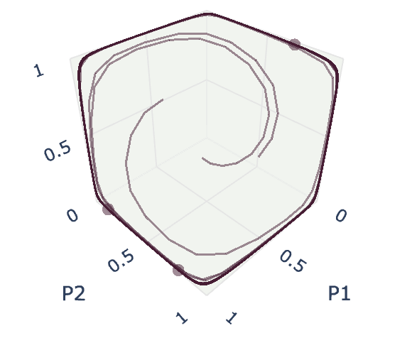
$T=0.7$

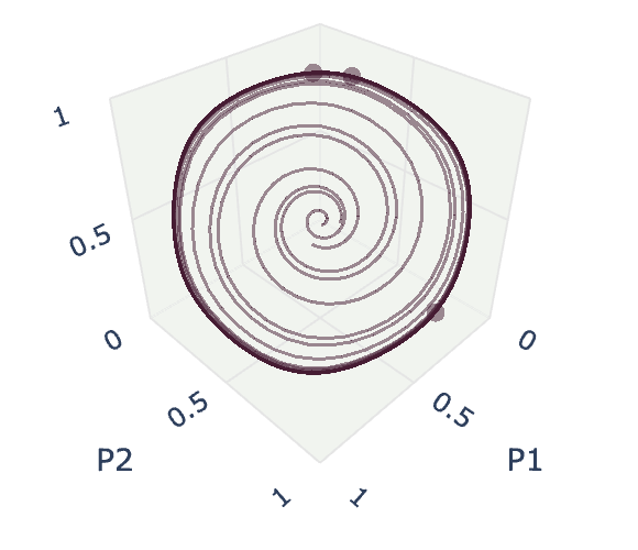
$T=1.5$

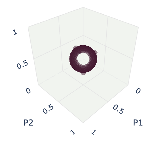
$T=2$

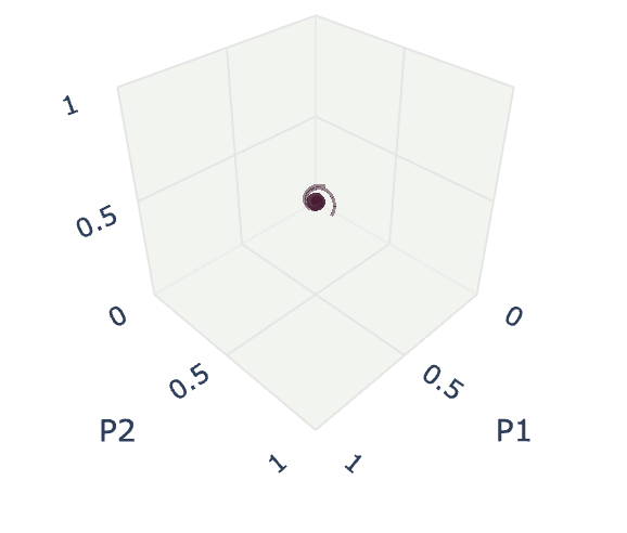
$T=2.7$

Figure 4. Trajectories of Q-Learning in a three agent Network Chakraborty Game with $\alpha=7,\beta=8.5$. Axes denote the probabilities with which each player chooses their first action.

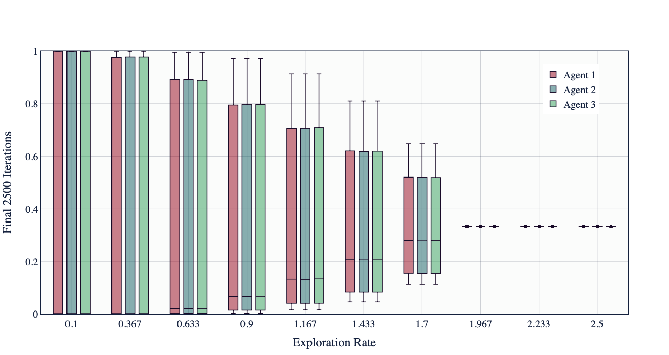
Fully Connected Network

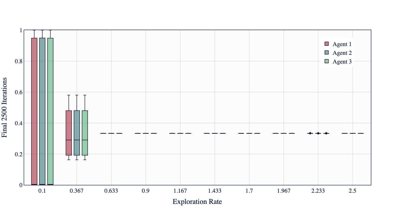
Ring Network

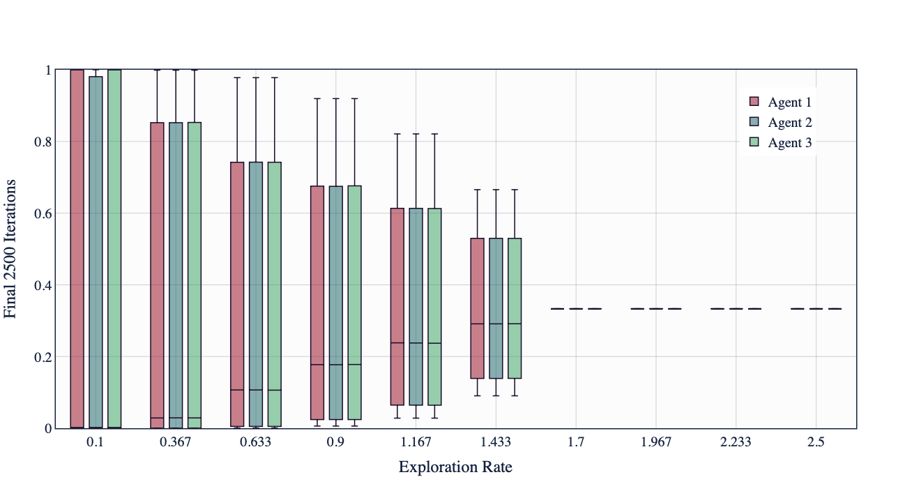
Fully Connected Network

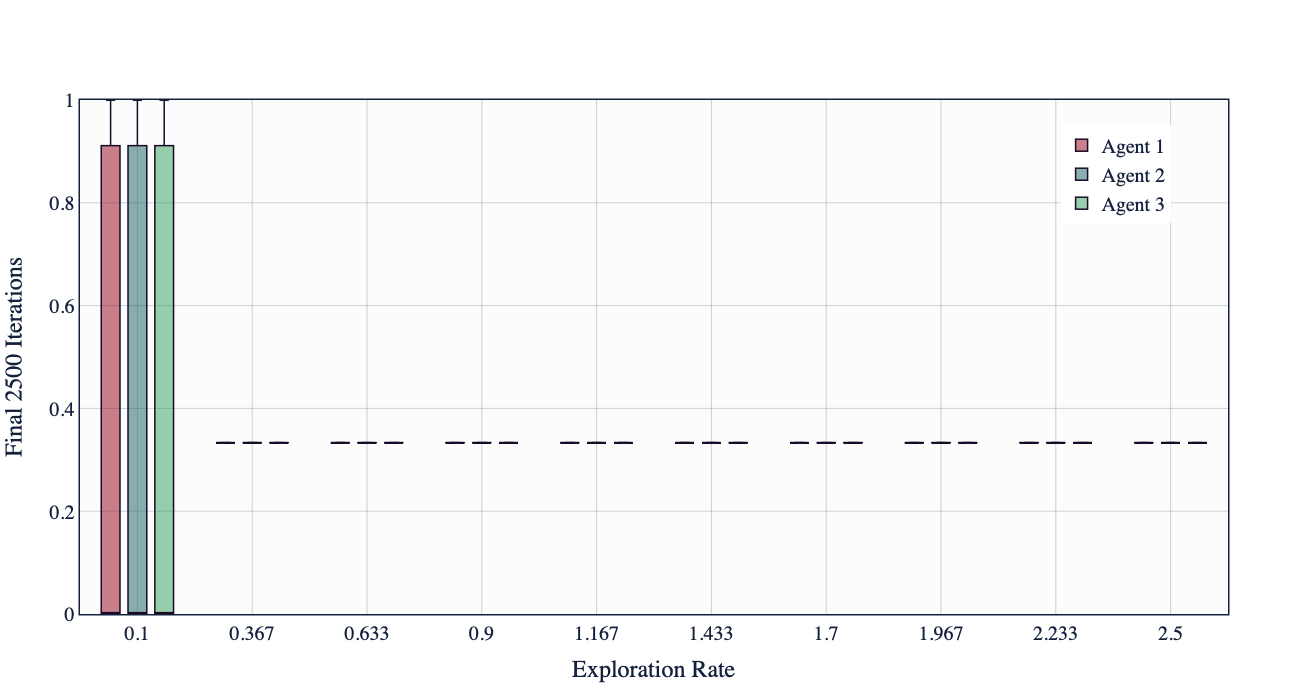
Ring Network

Figure 5. Q-Learning in the (Top) Network Shapley Game (Bottom) Network Sato Game with 15 agents. The boxplot depicts the probabilities with which three of the agents play their first action in the final 2500 iterations of learning. This is depicted for varying choices of exploration rate $T$.

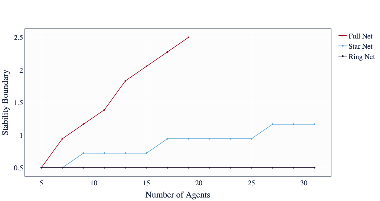
Shapley Game

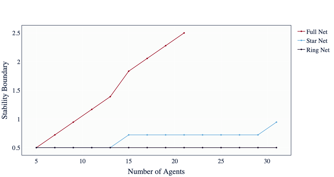
Sato Game

Figure 6. Empirically determined stability boundary of Q-Learning measured against the number of agents. Q-Learning is iterated with 10 initial conditions and the game is considered to have converged if, for all agents and initial conditions (6) holds with $l=1\times 10^{-5}$. The Fully Connected Network, Star Network and Ring Networks are considered.

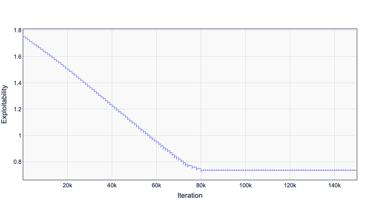
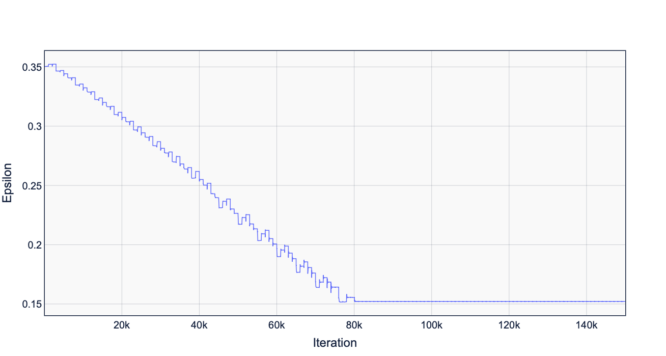
Figure 7. Measures of ‘closeness’ to Nash Equilibrium as the exploration update scheme is applied to the Network Chakraborty Game with five agents and $\alpha=2.5,\beta=1.5$. (Left) Distance to NE measured by exploitability (7) of the joint strategy $\mathbf{x}(t)$. (Right) $\epsilon$ as defined by (4). Both metrics decreases as exploration rates are updated until condition (6) fails at approx. $8\times 10^{4}$ iterations, after which learning is halted.

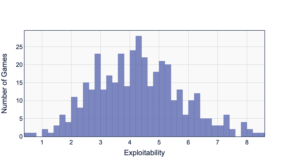
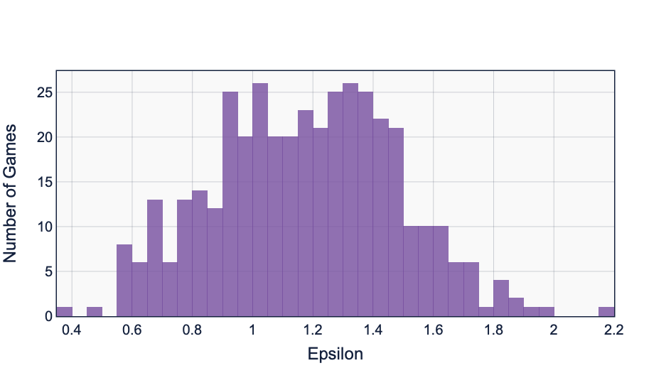
Figure 8. Histograms depicting the decrease of (Top) Exploitability and (Bottom) $\epsilon$ over $150,000$ iterations of learning across $500$ randomly generated network games with payoffs bounded in $[0,5]$.

We first visualise and exemplify the implications of our main result, Theorem 3.1, on a number of games. In particular, we simulate the Q-Learning algorithm described in Section 2.2 and show that Q-Learning asymptotically approaches a unique QRE so long as the exploration rates are sufficiently large. We show, in particular, that the amount of exploration required depends on the structure of the network rather than the total number of agents.

Remark 4.1.

In our experiments, we take all agents $k$ to have the same exploration rate $T$ and so drop the $k$ notation. As all bounds in Theorem 3.1 must hold for all agents $k$, this assumption does not affect the generality of the results.

4.1. Convergence of Q-Learning

We first illustrate the convergence of Q-Learning using the Network Chakraborty Game, which was analysed in Pandit et al. (2018) to characterise chaos in learning dynamics. Formally, the payoff to each agent $k$ is defined as

$$u_{k}(\mathbf{x}_{k},\mathbf{x}_{-k})=\mathbf{x}_{k}^{\top}\mathbf{A}\mathbf{x}_{l},\;l=k-1\mod N,$$

$$A=\begin{pmatrix}1&\alpha\\ \beta&0\end{pmatrix},\;\alpha,\beta\in\mathbb{R}.$$

We visualise the trajectories generated by running Q-Learning in Figure 4 for a three agent network and choosing $\alpha=7,\beta=8.5$. It can be seen that, for low exploration rates, the dynamics reach a limit cycle around the boundary of the simplex. However, as exploration increases, the dynamics are eventually driven towards a fixed point for all initial conditions.

Network Shapley Game

In the following example, each edge of the network game has associated the same pair of matrices $A,B$ where

$$A=\begin{pmatrix}1&0&\beta\\ \beta&1&0\\ 0&\beta&1\end{pmatrix},\,B=\begin{pmatrix}-\beta&1&0\\ 0&-\beta&1\\ 1&0&-\beta\end{pmatrix},$$

where $\beta\in(0,1)$.

This has been analysed in the two-agent case in Shapley (2016), where it was shown that the Fictitious Play learning dynamic do not converge to an equilibrium. Hussain et al. (2023b) analysed the network variant of this game for the case of a ring network and numerically showed that convergence can be achieved by Q-Learning through sufficient exploration.

In Figure 5 we examine both a fully connected network and a ring network with 15 agents. In this case, the dynamics evolve in $\mathbb{R}^{45}$ which prohibits a visualisation of the complete dynamics. To resolve this, we instead take three representative agents and depict the spread of their strategies in the final 2500 iterations of learning. A bar which stretches from $0$ to $1$ indicates that the dynamics are spread across the simplex which may occur in a limit cycle or chaotic orbit that approaches the boundary of the simplex (c.f. Figure 4). These are seen to occur for low exploration rates. By contrast, when exploration rates are increased beyond a certain threshold, a flat line is seen which indicates that the dynamics are stationary, i.e. a fixed point has been reached. Importantly, the boundary at which equilibrium behaviour occurs is higher in the fully connected network, where $\left\lVert G\right\rVert_{\infty}=14$ than in the ring network, where $\left\lVert G\right\rVert_{\infty}=2$. This indicates that larger numbers of agents may be introduced in the environment without impacting stability, so long as a weakly connected network is chosen.

Network Sato Game

We also analyse the behaviour of Q-Learning in a variant of the game introduced in Sato et al. (2002), where it was shown that chaotic behaviour is exhibited by learning dynamics in the two-agent case. We extend this towards a network game by associating each edge with the payoff matrices $A,B$ given by

$$A=\begin{pmatrix}\epsilon_{X}&-1&1\\ 1&\epsilon_{X}&-1\\ -1&1&\epsilon_{X}\end{pmatrix},\,B=\begin{pmatrix}\epsilon_{Y}&-1&1\\ 1&\epsilon_{Y}&-1\\ -1&1&\epsilon_{Y}\end{pmatrix},$$

where $\epsilon_{X},\epsilon_{Y}\in\mathbb{R}$. Notice that for $\epsilon_{X}=\epsilon_{Y}=0$, this corresponds to the classic Rock-Paper-Scissors game which is zero-sum so that, by Corollary 1, Q-Learning will converge to an equilibrium with any positive exploration rates. We choose $\epsilon_{X}=0.01,\epsilon_{Y}=-0.05$ in order to stay consistent with Sato et al. (2002) which showed chaotic dynamics for this choice. The boxplot once again shows that sufficient exploration leads to convergence of all initial conditions. However, the amount of exploration required is significantly smaller than that of the Network Shapley Game. This can be seen as being due to the significantly lower interaction coefficient of the Sato game $\sigma_{I}=0.05$ as compared to the Shapley game $\sigma_{I}=2$.

4.2. Stability Boundary

In these experiments we empirically determine the dependence of the stability boundary w.r.t. the number of agents. For accurate comparison with Figure 2, we consider the Network Sato and Shapley Games in a fully-connected network, star network and ring network. We iterate Q-Learning for various values of $T$ and determine whether the dynamics have converged. To evaluate convergence, we apply (6) with $|H|=2500$ iterations and $l=1\times 10^{-5}$. In Figure 6, we plot the smallest exploration rate $T$ for which (6) holds for varying choices of $N$. It can be seen that the prediction of Theorem 3.1 holds, in that the number of agents plays no impact for the ring network whereas the increase in the fully-connected network is linear in $N$. In addition, it is clear that the stability boundary increases slower in the Sato game than in the Shapley game, owing to the smaller interaction coefficient.

An additional point to note is that the stability boundary for the star network increases slower than the fully-connected network in all games. We anticipate that this is due to the fact that the $2$-norm $\lVert G\rVert_{2}$ in the star network is smaller than that of the fully-connected network (c.f. Figure 1).

4.3. Effectiveness of Exploration Update Scheme

In these experiments, we evaluate the exploration update scheme outlined in Section 3.2. using $|H|=500$ and $l=1\times 10^{-5}$. In Figure 7 we consider the Network Chakraborty Game with $\alpha=2.5,\beta=1.5$ We measure the ‘distance’ between the strategy $\mathbf{x}(t)$ and the NE using two metrics: first by $\epsilon$ as given in (4) and second through exploitability $\phi(\mathbf{x})$ given as

$$\phi(\mathbf{x})=\sum_{k}\max_{\mathbf{y}_{k}\in\Delta_{k}}u_{k}(\mathbf{y}_{k},\mathbf{x}_{-k})-u_{k}(\mathbf{x}_{k},\mathbf{x}_{-k}).$$ (7)

The exploitability is used, sometimes under different names, as a measure of distance to the NE Gemp et al. (2022); Perrin et al. (2020) and, from (4) it can be seen that $\phi(\mathbf{\bar{x}})=\sum_{k}T_{k}A_{k}(\mathbf{\bar{x}}_{k})$ for any QRE $\mathbf{\bar{x}}$. The reason for examining $\phi$ is that its definition holds for any strategy $\mathbf{x}\in\Delta$, whilst (4) only holds at a QRE $\mathbf{\bar{x}}\in\Delta$. It can be seen in all cases that both metrics decrease as agents learn, until condition (6) is no longer satisfied. To examine the generality of this performance, we evaluate the exploration update scheme in 500 randomly generated network games with 15 agents, two actions and a ring structure. Exploitability and $\epsilon$ are evaluated at the first iteration and final iteration and the difference is recorded. Figure 8 plots the decrease of both metrics as a histogram across all 500 games. These experiments (as well as additional presented in Appendix D) suggest that, if exploration rates are updated according the scheme in Section 3.2, independent learning agents may learn stable equilibrium strategies which closely approximate Nash Equilibria.

5. Conclusion

In this paper we show that the Q-Learning dynamics is guaranteed to converge in arbitrary network games, independent of any restrictive assumptions such as network zero-sum or potential. This allows us to make a branching statement which applies across all network games.

In particular, our analysis shows that convergence of the Q-Learning dynamics can be achieved through sufficient exploration, where the bound depends on the pairwise interaction between agents and the structure of the network. Overall, compared to the literature, we are able to tighten the bound on sufficient exploration and show that, under certain network interactions, the bound does not increase with the total number of agents. This allows for stability to be guaranteed in network games with many players.

A fruitful direction for future research would be to capture the effect of the payoffs through a tighter bound than the interaction coefficient and to explore further how properties of the network affect the bound. In addition, whilst there is still much to learn in the behaviour of Q-Learning in stateless games, the introduction of the state variable in the Q-update is a valuable next step.

Aamal Hussain and Francesco Belardinelli are partly funded by the UKRI Centre for Doctoral Training in Safe and Trusted Artificial Intelligence (grant number EP/S023356/1). Dan Leonte acknowledges support from the EPSRC Centre for Doctoral Training in Mathematics of Random Systems: Analysis, Modelling and Simulation (EP/S023925/1). This research was supported in part by the National Research Foundation, Singapore and DSO National Laboratories under its AI Singapore Program (AISG Award No: AISG2-RP-2020-016), grant PIESGP-AI-2020-01, AME Programmatic Fund (Grant No.A20H6b0151) from A*STAR.

Appendix A Preliminaries

In this section we outline the various tools and properties that we will use in our proofs.

A.1. Variational Inequalities and Monotone Games

Our aim in this work is to analyse the Q-Learning dynamics in network games without invoking any particular structure on the payoffs (e.g. zero-sum). To do this, we employ the Variational Inequality approach, which has been successfully applied towards the analysis of network games Melo (2018); Parise and Ozdaglar (2019) as well as learning in games Hadikhanloo et al. (2022); Sorin and Wan (2016); Hussain et al. (2023b).

Definition A.1 (Variational Inequality).

Consider a set $\mathcal{X}\subset\mathbb{R}^{d}$ and a map $F\,:\mathcal{X}\rightarrow\mathbb{R}^{d}$. The Variational Inequality (VI) problem $VI(\mathcal{X},F)$ is given as

$$\langle\mathbf{x}-\mathbf{\bar{x}},F(\mathbf{\bar{x}})\rangle\geq 0,\hskip 14.22636pt\text{ for all }\mathbf{x}\in\mathcal{X}.$$ (8)

We say that $\mathbf{\bar{x}}\in\mathcal{X}$ belongs to the set of solutions to a variational inequality problem $VI(\mathcal{X},F)$ if it satisfies (8).

The premise of the variational approach to game theory Facchinei and Pang (2004); Rosen (1965) is that the problem of finding equilibria of games can be reformulated as determining the set of solutions to a VI problem. This is done by choosing associating the set $\mathcal{X}$ with $\Delta$ and the map $F$ with the pseudo-gradient of the game.

Definition A.2 (Pseudo-Gradient Map).

The pseudo-gradient map of a game $\mathcal{G}=(\mathcal{N},\mathcal{E},(u_{k},\mathcal{S}_{k})_{k\in\mathcal{N}})$ is given by $F(\mathbf{x})=(F_{k}(\mathbf{x}))_{k\in\mathcal{N}}=(-D_{\mathbf{x}_{k}}u_{k}(\mathbf{x}_{k},\mathbf{x}_{-k}))_{k\in\mathcal{N}}$.

The advantage of this formulation is that we can apply results from the study of Variational Inequalities to determine properties of the game. These results rely solely on the form of the pseudo-gradient map and so can generalise results which assume a potential or zero-sum structure of the game Hussain et al. (2023b); Kadan and Fu (2021).

Lemma A.3 (Melo (2021)).

Consider a game $\mathcal{G}=(\mathcal{N},\mathcal{E},(u_{k},\mathcal{S}_{k})_{k\in\mathcal{N}})$ and for any $T_{1},\ldots,T_{N}>0$, let $F$ be the pseudo-gradient map of $\mathcal{G}^{H}$. Then $\mathbf{\bar{x}}\in\Delta$ is a QRE of $\mathcal{G}$ if and only if $\mathbf{\bar{x}}$ is a solution to $VI(\Delta,F)$.

With this correspondence in place, we can analyse properties of the pseudo-gradient map and its relation to properties of the game and the learning dynamic. One important property is monotonicity.

Definition A.4.

A map $F\,:\mathcal{X}\rightarrow\mathbb{R}^{d}$ is

1. Monotone if, for all $\mathbf{x},\mathbf{y}\in\mathcal{X}$,

   $$\langle F(\mathbf{x})-F(\mathbf{y}),\mathbf{x}-\mathbf{y}\rangle\geq 0.$$

2. Strongly Monotone with constant $\alpha>0$ if, for all $\mathbf{x},\mathbf{y}\in\mathcal{X}$,

   $$\langle F(\mathbf{x})-F(\mathbf{y}),\mathbf{x}-\mathbf{y}\rangle\geq\alpha||\mathbf{x}-\mathbf{y}||^{2}_{2}.$$

Definition A.5 (Monotone Game).

A game $\mathcal{G}$ is monotone if its pseudo-gradient map is monotone.

A large part of our analysis will be in determining conditions under which the pseudo-gradient map is monotone. Upon doing so, we are able to employ the following results.

Lemma A.6 (Melo (2021)).

Consider a game $\mathcal{G}=(\mathcal{N},\mathcal{E},(u_{k},\mathcal{S}_{k})_{k\in\mathcal{N}})$ and for any $T_{1},\ldots,T_{N}>0$, let $F$ be the pseudo-gradient map of $\mathcal{G}^{H}$. $\mathcal{G}$ has a unique QRE $\mathbf{\bar{x}}\in\Delta$ if $F$ is strongly monotone with any $\alpha>0$.

Lemma A.7 (Hussain et al. (2023b)).

If the game $G$ is monotone, then the Q-Learning Dynamics (QLD) converge to the unique QRE with any positive exploration rates $T_{1},\ldots,T_{N}>0$.

Finally, recall that an operator $f:\mathcal{X}\subset\mathbb{R}^{n}\rightarrow\mathbb{R}^{n}$ is strongly convex with constant $\alpha$ if, for all $\mathbf{x},\mathbf{y}\in\mathcal{X}$

$$f(\mathbf{y})\geq f(\mathbf{x})+Df(\mathbf{x})^{\top}(\mathbf{y}-\mathbf{x})+\frac{\alpha}{2}\lVert\mathbf{x}-\mathbf{y}\rVert^{2}_{2}.$$

It is known that, if $f(\mathbf{x})$ is strongly convex, then its Hessian $D^{2}_{\mathbf{x}}f(\mathbf{x})$ is strongly positive definite with constant $\alpha$. Thus, all eigenvalues of $D^{2}_{\mathbf{x}}f(\mathbf{x})$ are larger than $\alpha$. To apply this in our setting, we use the following result.

Proposition A.8 (Melo (2021)).

The function $f(\mathbf{x}_{k})=T_{k}\langle\mathbf{x}_{k},\ln\mathbf{x}_{k}\rangle$ is strongly convex with constant $T_{k}$.

A.2. Matrix Norms

In addition, the following definitions and properties hold for any matrix $A$.

1. $\lVert A\rVert_{2}=\sqrt{\lambda_{\max}(A^{\top}A)}$ where $\lambda_{\max}$ is the largest eigenvalue of $A$,

2. $\lVert A\rVert_{\infty}=\max_{i}\sum_{j}|[A]_{ij}|$,

3. $\rho(A)=\max_{i}|\lambda_{i}(A)|$ where $\lambda_{i}(A)$ denotes an eigenvalue of $A$.

Proposition A.9 (Weyl’s Inequality).

Let $J=D+N$ where $D$ and $N$ are symmetric matrices. Then it holds that

$$\lambda_{\min}(J)\geq\lambda_{\min}(D)+\lambda_{\min}(N).$$

where $\lambda_{\min}(A)$ denotes the smallest eigenvalue of a matrix.

Proposition A.10.

Let $G,A$ be matrices and $\otimes$ denote the Kronecker product. Then

$$\lVert G\otimes A\rVert_{2}=\lVert G\rVert_{2}\lVert A\rVert_{2}.$$

Proposition A.11.

Let $A$ be a symmetric matrix. Then

$$|\lambda_{\min}(A)|\leq\rho(A)=\lVert A\rVert_{2}.$$

The following result is used in our proof to be able to parameterise the effect of pairwise interactions by $\sigma_{I}$.

Lemma A.12.

Let $G\in\mathcal{M}_{N}(\mathbb{R})$ be matrix for which each entry $g_{ij}\vcentcolon=\left[G\right]_{ij}$ is either $0$ or $1$. Let $N\in\mathcal{M}_{Nn}(\mathbb{R})$ be a block matrix such that

$$\left[N\right]_{ij}=\begin{cases}A^{ij}&\text{ if }g_{ij}=1\\ \mathbf{0}&\text{ otherwise}\end{cases},$$

where $A^{ij}\in\mathcal{M}_{n}(\mathbb{R})$ are matrices of the same dimension. let $A\in M_{n}(\mathbb{R})$ be a matrix which satisfies $\lVert A\rVert_{2}\geq\lVert B^{ij}\rVert_{2}$ for all $(i,j)\in\mathcal{E}$. Finally let $\tilde{N}\in M_{Nn}(\mathbb{R})$ be a block matrix given by Then

$$\left\lVert N\right\rVert_{2}\leq\sqrt{\left\lVert G\right\rVert_{1}\left\lVert G\right\rVert_{\infty}}\max_{1\leq i,j\leq n}\left\lVert A_{ij}\right\rVert_{2}.$$

Proof.

Let $v=(v^{1},\ldots,v^{n})\in\mathbb{R}^{Nn}$ where $v^{i}\in\mathbb{R}^{N}$ for $1\leq i\leq n$. Then

$$\lVert Nv\rVert_{2}^{2}=\left\lVert\begin{pmatrix}g_{11}A^{11}&\ldots&g_{1n}A^{1n}\\ \vdots&&\vdots\\ g_{n1}A^{n1}&\ldots&g_{nn}A^{nn}\end{pmatrix}\begin{bmatrix}v^{1}\\ \vdots\\ v^{n}\end{bmatrix}\right\rVert_{2}^{2}=\left\lVert\begin{bmatrix}\sum_{1j}g_{1j}A^{1j}v^{j}\\ \vdots\\ \sum_{ni}g_{nj}A^{nj}v^{j}\end{bmatrix}\right\rVert_{2}^{2}\leq\sum_{i=1}^{n}\left\lVert\sum_{j=1}^{n}g_{ij}A^{ij}v^{j}\right\rVert_{2}^{2}.$$ (9)

For each fixed $i\in\{1,\ldots,n\}$, we have the upper bound

$$\left\lVert\sum_{j=1}^{n}g_{ij}A^{ij}v^{j}\right\rVert_{2}\leq\sum_{j=1}^{n}g_{ij}\left\lVert A^{ij}v^{j}\right\rVert_{2}\leq\sum_{j=1}^{n}g_{ij}\left\lVert A^{ij}\right\rVert_{2}\left\lVert v^{j}\right\rVert_{2}\leq\max_{1\leq i,j\leq n}\left\lVert A^{ij}\right\rVert_{2}\sum_{j=1}^{n}g_{ij}\left\lVert v^{j}\right\rVert_{2}.$$ (10)

By plugging (10) in (9) and expanding the squared bracket, we obtain that

$$\lVert Nv\rVert_{2}^{2}\leq\sum_{i=1}^{n}\left(\max_{1\leq i,j\leq n}\left\lVert A^{ij}\right\rVert_{2}\sum_{j=1}^{n}g_{ij}\left\lVert v^{j}\right\rVert_{2}\right)^{2}= \max_{1\leq i,j\leq n}\left\lVert A^{ij}\right\rVert_{2}^{2}\sum_{i=1}^{n}\sum_{k,l=1}^{n}g_{ik}g_{il}\left\lVert v^{k}\right\rVert_{2}\left\lVert v^{l}\right\rVert_{2}$$

$$\leq \max_{1\leq i,j\leq n}\left\lVert A^{ij}\right\rVert_{2}^{2}\sum_{i=1}^{n}\sum_{k,l=1}^{n}g_{ik}g_{il}\left(\frac{1}{2}\left\lVert v^{k}\right\rVert_{2}^{2}+\frac{1}{2}\left\lVert v^{l}\right\rVert_{2}^{2}\right),$$

where the last inequality follows by completing the square. Notice that the two sums above are identical, hence

$$\lVert Nv\rVert_{2}^{2}\leq\max_{1\leq i,j\leq n}\left\lVert A^{ij}\right\rVert_{2}^{2}\sum_{i=1}^{n}\sum_{k,l=1}^{n}g_{ik}g_{il}\left\lVert v^{k}\right\rVert_{2}^{2}.$$

It remains the upper bound the RHS in the above inequality. Indeed, we have that

$$\sum_{i=1}^{n}\sum_{k,l=1}^{n}g_{ik}g_{il}\left\lVert v^{k}\right\rVert_{2}^{2} =\sum_{i=1}^{n}\sum_{k=1}^{n}g_{ik}\left\lVert v^{k}\right\rVert_{2}^{2}\left(\sum_{l=1}^{n}g_{il}\right)\leq\left\lVert G_{\infty}\right\rVert\sum_{i=1}^{n}\sum_{k=1}^{n}g_{ik}\left\lVert v^{k}\right\rVert_{2}^{2}$$

$$\leq\left\lVert G_{\infty}\right\rVert\sum_{k=1}^{n}\left(\sum_{i=1}^{n}g_{ik}\right)\left\lVert v^{k}\right\rVert_{2}^{2}\leq\left\lVert G_{\infty}\right\rVert\left\lVert G_{1}\right\rVert\sum_{k=1}^{n}\left\lVert v^{k}\right\rVert_{2}^{2}=\left\lVert G_{\infty}\right\rVert\left\lVert G_{1}\right\rVert.$$

Thus

$$\sup_{v\colon\left\lVert v\right\rVert=1}\left\lVert Nv\right\rVert_{2}^{2}\leq\left\lVert G_{\infty}\right\rVert\left\lVert G_{1}\right\rVert\max_{i,j}\left\lVert A^{ij}\right\lVert_{2}^{2},$$

and the conclusion follows.

∎

Appendix B Proof of Theorem 3.1

In this section we provide the full proof of Theorem 3.1. First, we prove the following result, which will be used to parameterise interactions by the influence bound $\delta_{k}$.

Lemma B.1.

In a network game $\mathcal{G}=(\mathcal{N},\mathcal{E},(u_{k},\mathcal{S}_{k})_{k\in\mathcal{N}})$, the following holds for any agent $k\in\mathcal{N}$ action $i\in\mathcal{S}_{k}$ and strategies $\mathbf{x}_{-k},\mathbf{y}_{-k}\in\Delta_{-k}$

$$|r_{ki}(\mathbf{x}_{-k})-r_{ki}(\mathbf{y}_{-k})|\leq\delta_{k}\sum_{l\in\mathcal{N}_{k}}\lVert\mathbf{x}_{l}-\mathbf{y}_{l}\rVert_{1}.$$

Proof.

Fix an agent $k$ and define the dummy game $\tilde{\mathcal{G}}_{k}=(\mathcal{N}_{k}\cup\{k\},(\tilde{u}_{k},\mathcal{S}_{k})_{k\in\mathcal{N}_{k}\cup\{k\}})$ so that $\tilde{\mathcal{G}}_{k}$ is composed of only agent $k$ and its neighbours. In addition, the rewards are chosen so that $\tilde{r}_{ki}(\mathbf{x}_{-k})=r_{ki}(\mathbf{x}_{-k})$ for all $\mathbf{x}_{-k}$ and $\tilde{r}_{li}(\mathbf{x}_{-l})=\tilde{r}_{lj}(\mathbf{x}_{-l})$ for all $l\in\mathcal{N}_{k}$ and all $i,j\in\mathcal{S}_{k}$. In $\tilde{\mathcal{G}}_{k}$, the maximum influence bound $\delta:=\max_{l\in\mathcal{N}_{k}\cup\{k\}}\delta_{l}$ is exactly $\delta_{k}$. Then, from Cominetti et al. (2010) Proposition 5, the following holds in $\tilde{\mathcal{G}}_{k}$

$$|r_{ki}(\mathbf{x}_{-k})-r_{ki}(\mathbf{y}_{-k})|\leq\sum_{l\neq k}\delta\lVert\mathbf{x}_{l}-\mathbf{y}_{l}\rVert_{1}.$$

This translates in the original network game $\mathcal{G}$ to the statement of the Lemma. ∎

With these results in place, we can prove Theorem 3.1 in the main paper.

Proof of Theorem 3.1.

In order to apply Lemma A.7 we show that, under any of the conditions, the perturbed game $\mathcal{G}^{H}$ is strongly monotone. To this end, we take the derivative of the pseudo-gradient of $\mathcal{G}^{H}$ which we call the pseudo-Hessian given by

$$[J(\mathbf{x})]_{k,l}=D_{\mathbf{x}_{l}}F_{k}(\mathbf{x}).$$

It follows that, if $\frac{J(\mathbf{x})+J^{\top}(\mathbf{x})}{2}$ is strongly positive definite for all $\mathbf{x}\in\Delta$ with any $\alpha>0$, i.e. $\mathbf{x}^{\top}J(\mathbf{x})\mathbf{x}\geq\alpha$ for all $\mathbf{x}\in\Delta$, then $F(\mathbf{x})$ is strongly monotone with the same constant $\alpha$. We can rewrite the pseudo-Hessian as

$$J(\mathbf{x})=D(\mathbf{x})+N(\mathbf{x}),$$

where $D(\mathbf{x})$ is a block diagonal matrix with $-D^{2}_{\mathbf{x}_{k}\mathbf{x}_{k}}u_{k}^{H}(\mathbf{x}_{k},\mathbf{x}_{-k})$ along the diagonal. $N(\mathbf{x})$ is an off-diagonal block matrix with

$$[N(\mathbf{x})]_{k,l}=\begin{cases}-D_{\mathbf{x}_{k},\mathbf{x}_{l}}u_{k}^{H}(\mathbf{x}_{k},\mathbf{x}_{-k})&\text{ if }(k,l)\in\mathcal{E}\\ \mathbf{0}&\text{ otherwise}\end{cases}.$$

In words, $N(x)$ shares the same structure of the adjacency matrix $G$ of the game, except that it has $-D_{\mathbf{x}_{k},\mathbf{x}_{l}}u_{k}^{H}(\mathbf{x}_{k},\mathbf{x}_{-k})$ wherever $G$ takes the value $1$ and the block matrix $\mathbf{0}$ wherever $G$ has $0$. Next we evaluate these partial differentials. Recall that

$$-u_{k}^{H}(\mathbf{x}_{k},\mathbf{x}_{-k})=T_{k}\langle\mathbf{x}_{k},\ln\mathbf{x}_{k}\rangle-\sum_{(k,l)\in\mathcal{E}}\mathbf{x}_{k}\cdot A^{kl}\mathbf{x}_{l}.$$

As a result, for all $(k,l)\in\mathcal{E}$, $\left[N(\mathbf{x})\right]_{k,l}=-A^{kl}$, so that $N(\mathbf{x})$ represents the network interaction. By contrast, $D(\mathbf{x})$ depends on $T_{k}$ and is independent of the payoffs $u_{k}$. As such, it measures the strength of the game perturbation. Now, let $\bar{J}(\mathbf{x})$ be defined as

$$\bar{J}(\mathbf{x})=\frac{J(\mathbf{x})+J^{\top}(\mathbf{x})}{2}=D(\mathbf{x})+\frac{N(\mathbf{x})+N^{\top}(\mathbf{x})}{2}.$$

Then, from Proposition A.8 it follows that $D(\mathbf{x})$ is strongly positive definite with constant $T=\min_{k}T_{k}$. In particular, this means that $\lambda_{\min}D(\mathbf{x})\geq T$. Finally, applying Weyl’s inequality

$$\lambda_{\min}(\bar{J}) \geq T+\lambda_{\min}\left(\frac{N+N^{\top}}{2}\right)$$

$$\geq T-\rho\left(\frac{N+N^{\top}}{2}\right)$$

$$=T-\left\lVert\frac{N+N^{\top}}{2}\right\rVert_{2}$$

$$\geq T-\frac{1}{2}\left\lVert A+B\right\lVert_{2}\sqrt{\lVert G\rVert_{\infty}\lVert G\rVert_{1}}$$

$$=T-\frac{1}{2}\left\lVert A+B^{\top}\right\rVert_{2}\left\lVert G\right\rVert_{\infty}$$

$$=T-\frac{1}{2}\sigma_{I}\left\lVert G\right\rVert_{\infty},$$

where we employ Propositions A.11, Lemma A.12 and the fact that $G$ is symmetric so that $\lVert G\rVert_{\infty}=\lVert G\rVert_{1}$. The matrices $A,B$ are chosen so that

$$\left\lVert A+B^{\top}\right\rVert_{2}=\max_{(k,l)\in\mathcal{E}}\left\lVert A^{kl}+(A^{lk})^{\top}\right\rVert_{2}=\sigma_{I}.$$

Then, under (C2), $\lambda_{\min}(\bar{J}(\mathbf{x}))\geq T-\frac{1}{2}\sigma_{I}\lVert G\rVert_{\infty}>0$ and, therefore $F(\mathbf{x})$ is strongly monotone with constant $T-\frac{1}{2}\sigma_{I}\left\lVert G\right\rVert_{\infty}$. Using Lemma A.7, it follows that Q-Learning Dynamics converge to a unique QRE.

To achieve (C3) we apply Proposition A.10 which yields that

$$T-\left\lVert\frac{N+N^{\top}}{2}\right\rVert_{2}$$

$$= T-\left\lVert\frac{(A+B^{\top})\otimes G}{2}\right\rVert_{2}$$

$$= T-\frac{1}{2}\left\lVert A+B^{\top}\right\rVert_{2}\left\lVert G\right\rVert_{2}$$

$$= T-\frac{1}{2}\sigma_{I}\left\lVert G\right\rVert_{2}.$$

Finally, we prove (C1). In this case, it holds that, for any $k$ and any $\mathbf{x},\mathbf{y}\in\Delta$

$$(\mathbf{x}_{k}-\mathbf{y}_{k})^{\top}(F_{k}(\mathbf{x})-F_{k}(\mathbf{y})) =(\mathbf{x}_{k}-\mathbf{y}_{k})^{\top}(T_{k}\ln\mathbf{x}_{k}-T_{k}\ln\mathbf{y}_{k})-(\mathbf{x}_{k}-\mathbf{y}_{k})^{\top}(T_{k}r_{k}(\mathbf{x}_{-k})-T_{k}r_{k}(\mathbf{y}_{-k}))$$

$$\geq T_{k}\lVert\mathbf{x}_{k}-\mathbf{y}_{k}\rVert_{1}^{2}-\left|(\mathbf{x}_{k}-\mathbf{y}_{k})^{\top}\left(r_{k}(\mathbf{x}_{-k})-r_{k}(\mathbf{y}_{-k})\right)\right|$$

$$\geq T_{k}\lVert\mathbf{x}_{k}-\mathbf{y}_{k}\rVert_{1}^{2}-\lVert\mathbf{x}_{k}-\mathbf{y}_{k}\rVert_{1}\delta_{k}\sum_{l\in\mathcal{N}_{k}}\lVert\mathbf{x}_{l}-\mathbf{y}_{l}\rVert_{1}$$

$$\geq T_{k}\lVert\mathbf{x}_{k}-\mathbf{y}_{k}\rVert_{1}^{2}-\lVert\mathbf{x}_{k}-\mathbf{y}_{k}\rVert_{1}\delta_{k}\sum_{l\neq k}[G]_{kl}\lVert\mathbf{x}_{l}-\mathbf{y}_{l}\rVert_{1}$$

$$=\xi_{k}(M\xi)_{k},$$

where $\xi=(\mathbf{x}_{k}-\mathbf{y}_{k})_{k\in\mathcal{N}}$ and $M=(diag(T_{k})_{k\in\mathcal{N}}-diag(\delta_{k})_{k\in\mathcal{N}}\cdot G)$. Notice that, to achieve the third inequality, we applied Lemma B.1 Then under (C1), $M$ is strictly diagonally dominant and so is strictly positive definite. Then

$$\sum_{k}(\mathbf{x}_{k}-\mathbf{y}_{k})^{\top}(F_{k}(\mathbf{x})-F_{k}(\mathbf{y}))\geq\xi^{\top}M\xi>0,$$

so that $F(\mathbf{x})$ is strictly monotone. Then, Lemma A.7 can be applied to yield convergence of Q-Learning Dynamics. ∎

Appendix C Proofs from Section 3.1

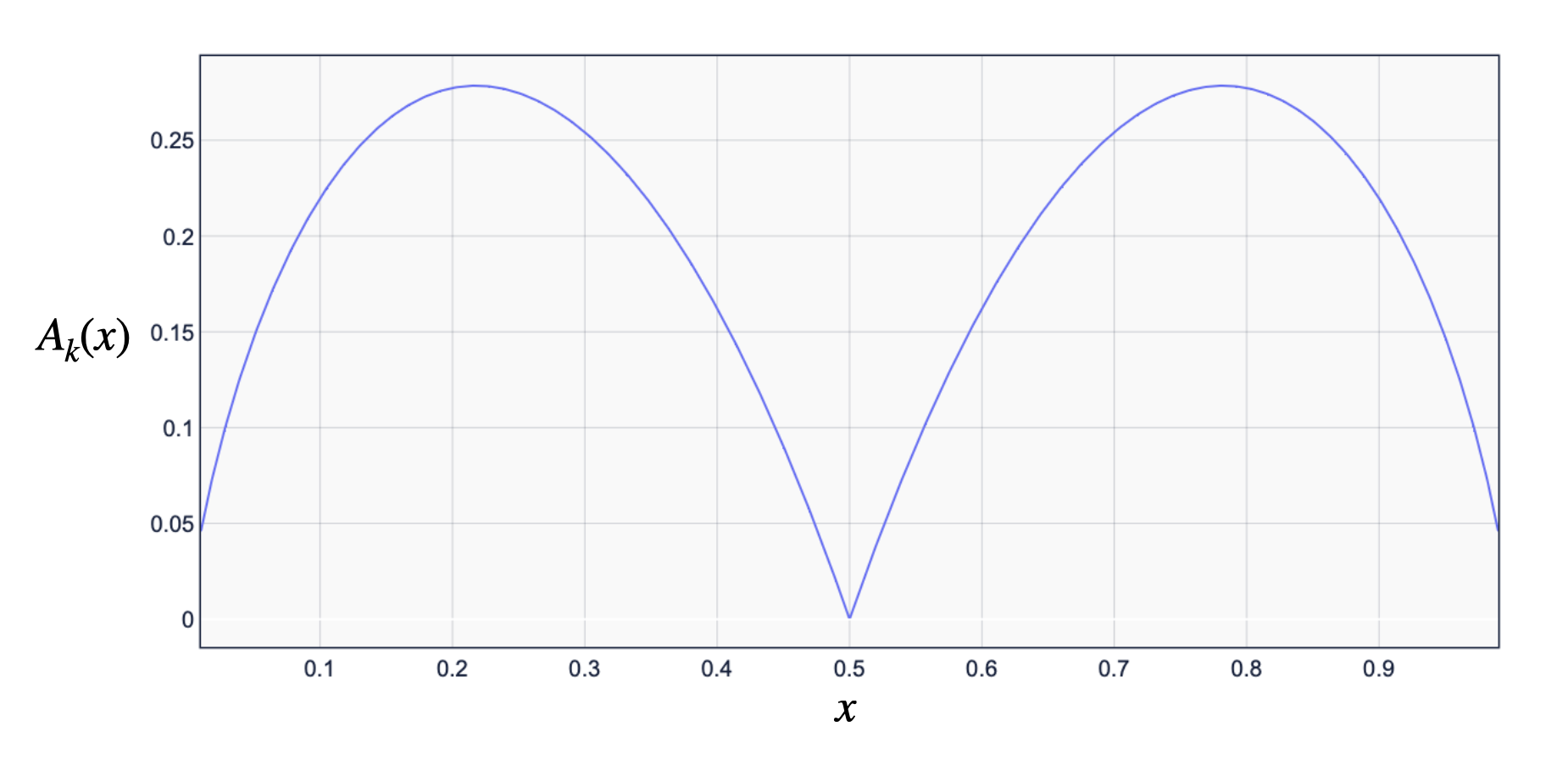
$n_{k}=2$

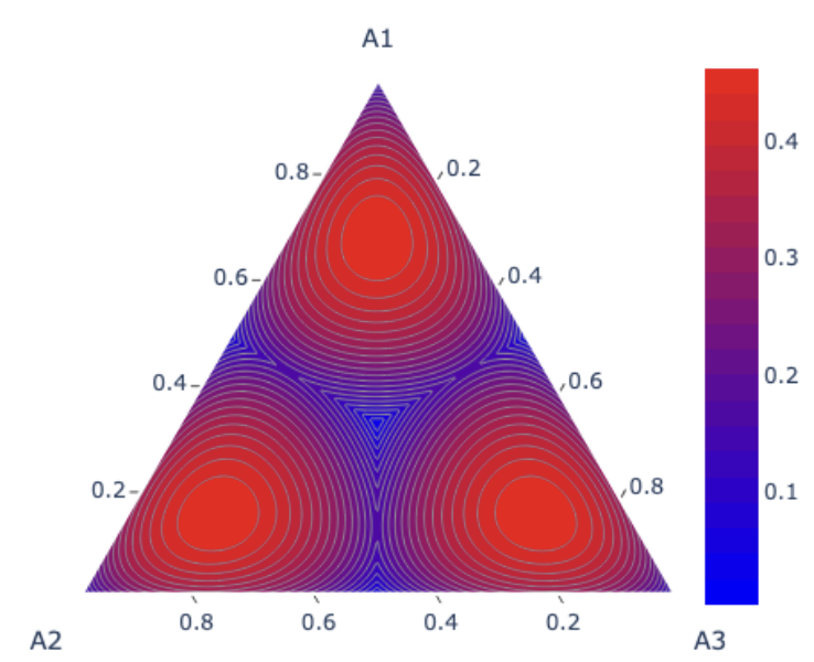
$n_{k}=3$

Figure 9. $A_{k}(\mathbf{x}_{k})$ plotted on a unit simplex $\Delta_{k}$

First we show that any QRE $\mathbf{\bar{x}}$ is an approximate Nash Equilibrium.

Proof of Proposition 3.8.

We first notice that, for some $\epsilon>0$, the definition of an $\epsilon$-Nash Equilibrium in Definition 3.7 holds if

$$\max_{k\in\mathcal{N}}\max_{i\in\mathcal{S}_{k}}r_{ki}(\mathbf{\bar{x}}_{-k})-\langle\mathbf{\bar{x}}_{k},r_{k}(\mathbf{\bar{x}}_{-k})\rangle=\epsilon.$$

Next, recall that a QRE $\mathbf{\bar{x}}\in\Delta$ corresponds to an interior fixed point of the Q-Learning Dynamics Leonardos et al. (2021). From this it holds that, for any $k$ and any $i\in\mathcal{S}_{k}$

$$0 =r_{ki}(\mathbf{\bar{x}}_{-k})-\langle\mathbf{\bar{x}}_{k},r_{k}(\mathbf{\bar{x}}_{-k})\rangle+T_{k}\sum_{j\in\mathcal{S}_{k}}\bar{x}_{kj}\ln\frac{x_{kj}}{x_{ki}}$$

$$r_{ki}(\mathbf{\bar{x}}_{-k})-\langle\mathbf{\bar{x}}_{k},r_{k}(\mathbf{\bar{x}}_{-k})\rangle =-T_{k}\sum_{j\in\mathcal{S}_{k}}\bar{x}_{kj}\ln\frac{x_{kj}}{x_{ki}}$$

$$=T_{k}\ln x_{ki}-\langle\mathbf{x}_{k},\ln\mathbf{x}_{k}\rangle.$$

As this holds for any $i\in\mathcal{S}_{k}$, the following holds

$$\max_{k\in\mathcal{N}}\max_{i\in\mathcal{S}_{k}}r_{ki}(\mathbf{\bar{x}}_{-k})-\langle\mathbf{\bar{x}}_{k},r_{k}(\mathbf{\bar{x}}_{-k})\rangle =\max_{k\in\mathcal{N}}T_{k}\max_{i\in\mathcal{S}_{k}}\ln x_{ki}-\langle\mathbf{x}_{k},\ln\mathbf{x}_{k}\rangle$$

$$=\max_{k\in\mathcal{N}}T_{k}A_{k}(\mathbf{\bar{x}}_{k}),$$

so that $\mathbf{\bar{x}}$ is an $\epsilon$-Nash Equilibrium with $\epsilon=\max_{k\in\mathcal{N}}T_{k}A_{k}(\mathbf{\bar{x}}_{k})$ ∎

Lemma C.1 (Full version of Lemma 3.11).

Let $\mathbf{u}_{k}=(1/n_{k},\ldots,1/n_{k})\in\Delta_{k}$ and $\mathbf{e}_{ki}\in\Delta_{k}$ be the canonical basis vector with $i^{\text{th}}$ entry equal to $1$ and $0$ elsewhere. Then

$$\bar{A}_{k}:=\max_{\mathbf{x}_{k}\in\Delta_{k}}\left(\max_{i\in\mathcal{S}_{k}}\ln{x_{ki}}-\sum_{j\in\mathcal{S}_{k}}x_{kj}\ln{x_{kj}}\right)=\frac{\ln{(n_{k}-1)}-\ln\left(W\left(\frac{n_{k}-1}{e}\right)\right)}{1+1/W\left(\frac{n_{k}-1}{e}\right)},$$ (11)

with equality if $\mathbf{x}^{*}=c\,\mathbf{e}_{ki}+(1-c)\mathbf{u}_{k}\,$ for any $i\in\mathcal{S}_{k}$, where $c=1/\left(W\left(\frac{n_{k}-1}{e}\right)+1\right)$ and $W(\cdot)$ is the Lambert W function.

Proof.

The $\max$ over $i\in\{1,\ldots,n_{k}\}$ can be eliminated, as

$$\max_{\mathbf{x}_{k}\in\Delta_{k}}\left(\max_{i\in\mathcal{S}_{k}}\ln{x_{ki}}-\sum_{j\in\mathcal{S}_{k}}x_{kj}\ln{x_{kj}}\right)=\max_{\mathbf{x}_{k}\in\Delta_{k}}\left(\ln{x_{ki}}-\sum_{j\in\mathcal{S}_{k}}x_{kj}\ln{x_{kj}}\right).$$ (12)

Notice that any value of the LHS realized by $\mathbf{x}_{k}$ can also be realized by the RHS for $\mathbf{y}_{k}$, where $\mathbf{y}_{k}$ is obtained from $\mathbf{x}_{k}$ by swapping the largest and $i^{\text{th}}$ entries of $\mathbf{x}_{k}$. Explicitly, let $i_{0}=\arg\max_{j\in\mathcal{S}_{k}}x_{kj}$ and

$$y_{kj}=\begin{cases}x_{ki_{0}}&\text{ if }j=i\\ x_{ki}&\text{ if }j=i_{0}\\ x_{kj}&\text{ otherwise }\end{cases}$$

Having eliminated the inner maximization, we can formulate the RHS of (12) as a constrained optimization problem, which we solve in two steps.

Firstly, we show that the $\mathbf{x}^{*}$ maximizing the RHS of (12) lies on one of the line segments connecting the vertices $\mathbf{e}_{ki}$ of the simplex $\Delta_{k}$ with the uniform distribution $\mathbf{u}_{k}$ (see Figure 9). Next, we determine the position of $\mathbf{x}^{*}$ on this segment, and substitute the value of $\mathbf{x}^{*}$ to obtain the RHS of (11). We then derive tight bounds on this quantity.

For the first step, consider the Lagrangian $L\colon\Delta_{k}\times(0,-\infty)\rightarrow\mathbb{R}\cup\{\infty\}$ given by

$$L\left(\mathbf{x}_{k}\right)=\ln{x_{ki}}-\sum_{j\in\mathcal{S}_{k}}x_{kj}\ln{x_{kj}}+\lambda\left(\sum_{j\in\mathcal{S}_{k}}x_{kj}-1\right).$$

Setting the partial derivatives to $0$, we obtain that

$$\frac{\partial L}{\partial x_{ki}} =-1+\lambda+1/x_{kj}-\ln{x_{i}}=0,$$

$$\frac{\partial L}{\partial x_{kj}} =-1+\lambda-\ln{x_{kj}}=0\text{ for all }j\in\mathcal{S}_{k}\text{ with }j\neq i,$$

$$\frac{\partial L}{\partial\lambda} =\sum_{j\in\mathcal{S}_{k}}x_{kj}-1=0,$$

with the solution given by $\mathbf{x}^{*}$ with $x_{kj}=1/W(e^{1-\lambda})$ and $x_{ki}=e^{-1+\lambda}$ for $j\neq i$, where $W$ is the Lambert W function. Note that $L(\mathbf{x}_{k})=-\infty$ for $\mathbf{x}_{k}$ on the boundary of $\Delta_{k}$ and further that the mapping $\mathbf{x}_{k}\to\ln{x_{ki}}-\sum_{j\in\mathcal{S}_{k}}x_{kj}\ln{x_{kj}}$ is concave, as its Hessian is diagonal with negative entries, hence the stationary point of $L$ gives a maximum. Finally, determining $\lambda$ is equivalent to solving

$$\sum_{j\in\mathcal{S}_{k}}x_{kj}=\frac{1}{W(e^{1-\lambda})}+(n_{k}-1)e^{-1+\lambda}=1,$$

which is intractable to the best of our knowledge, even with modern software such as Mathematica. Nevertheless, we have proved that the maximizer $\mathbf{x}^{*}$ of (12) lies on the line segment connecting a vertex and the centre of the simplex, which reduces our initial constrained optimization problem to one dimension. Without loss of generality, pick the first vertex and let $\mathbf{x}^{*}=(x,\frac{1-x}{n_{k}-1},\ldots,\frac{1-x}{n_{k}-1})$ for some $x\in[0,1]$. We have that

$$\ln{x_{i}}-\sum_{j\in\mathcal{S}_{k}}x_{kj}\ln{x_{kj}}=\ln{x}+x\ln{x}+(1-x)\ln{\frac{1-x}{n_{k}-1}},$$

which involves no special functions. By setting the derivative to $0$, we find that this expression is maximized for $x=1/\left(1+W\left(\frac{n_{k}-1}{e}\right)\right)$ and that the maximum value is given by

$$\bar{A}_{k}=\frac{\ln{(n_{k}-1)}-\ln\left(W\left(\frac{n_{k}-1}{e}\right)\right)}{1+1/W\left(\frac{n_{k}-1}{e}\right)}.$$

Finally, we give bounds for $\bar{A}_{k}$. Hoorfar and Hassani (2008) proves the sharp bound

$$\ln{x}-\ln{\ln{x}}<W(x)<\ln{x}-\ln{\ln{x}}+\ln{(1+1/e)},$$

which translates to

$$\bar{A}_{k}<\frac{\ln{n_{k}}-\ln{\left(\ln{n_{k}}-\ln{\ln{n_{k}}}\right)}}{1+\frac{1}{\ln n_{k}-\ln{\ln{n_{k}}}}}<\ln{n_{k}}-\ln{\left(\ln{n_{k}}-\ln{\ln{n_{k}}}\right)}<\ln n_{k}.$$

∎

Algorithm 1 Iterative improvement of QRE

Appendix D Additional Experiments

In this section, we present additional experiments on the behaviour of Q-Learning in Network Games, as well as on the exploration update scheme. In Figure 10, we examine a Network Mismatching Game, which was analysed in Kleinberg et al. (2011) as an example of limit cycle behaviour in replicator dynamics. Here, the payoff to each agent $k$ is given as

$$u_{k}(\mathbf{x}_{k},\mathbf{x}_{-k})=\mathbf{x}_{k}^{\top}\mathbf{A}\mathbf{x}_{l},\;l=k-1\mod N,$$

$$A=\begin{pmatrix}0&1\\ M&0\end{pmatrix},\;M\geq 1$$

From Figure 10 it is clear that, as exploration rates increase, the dynamics are driven towards a QRE from all initial conditions.

Next, we present additional experiments on the exploration updating scheme in Section 3.2. In particular, we apply the scheme to a Network Mismatching Game with 5 agents. We plot the exploitability (7) and $\epsilon$ (4) over $150,000$ iterations of learning. In both cases it is again clear that the distance to Nash decreases as the exploration updating scheme is applied. In the case that $M=2$, the scheme is applied until (6) fails at approx. $60,000$ iterations, whilst in the case $M=4$, agents learn for $80,000$ iterations before the dynamics are considered unstable. In Figure 12 we plot the trajectories of Q-Learning using the first action played by three representative agents. The dynamics move between QRE as the exploration rates are adjusted, however stability of the dynamic is maintained.

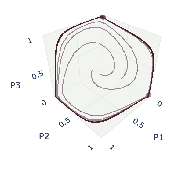
$T=0.15$

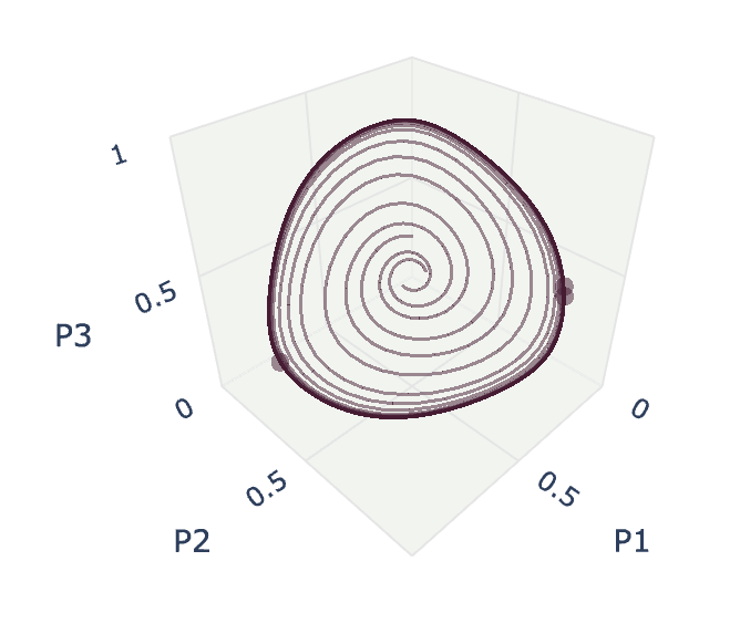
$T=0.3$

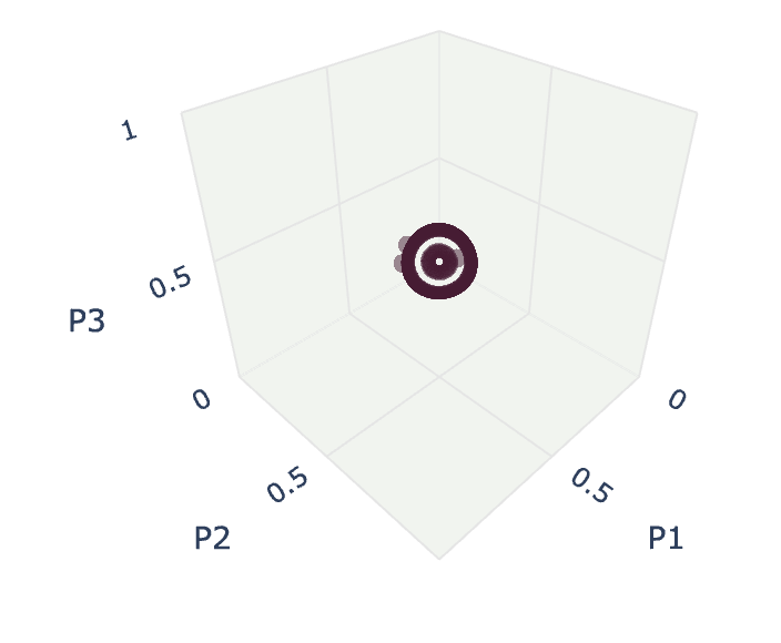
$T=0.4$

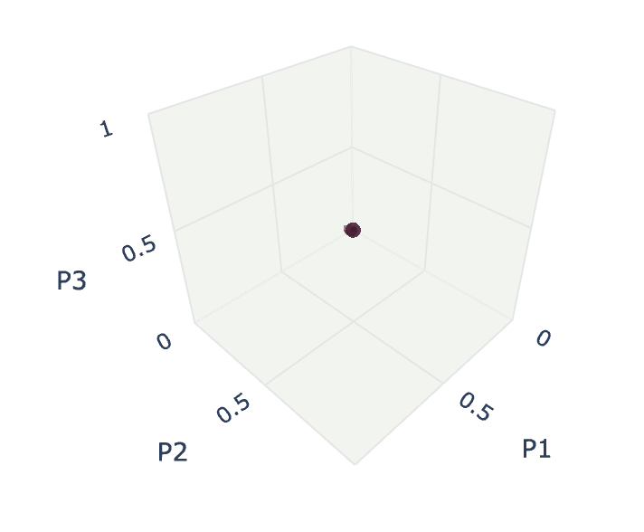
$T=0.55$

Figure 10. Trajectories of Q-Learning in a three agent Network Mismatching Game with $M=2$. Axes denote the probabilities with which each player chooses their first action.

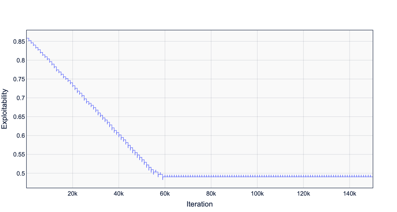
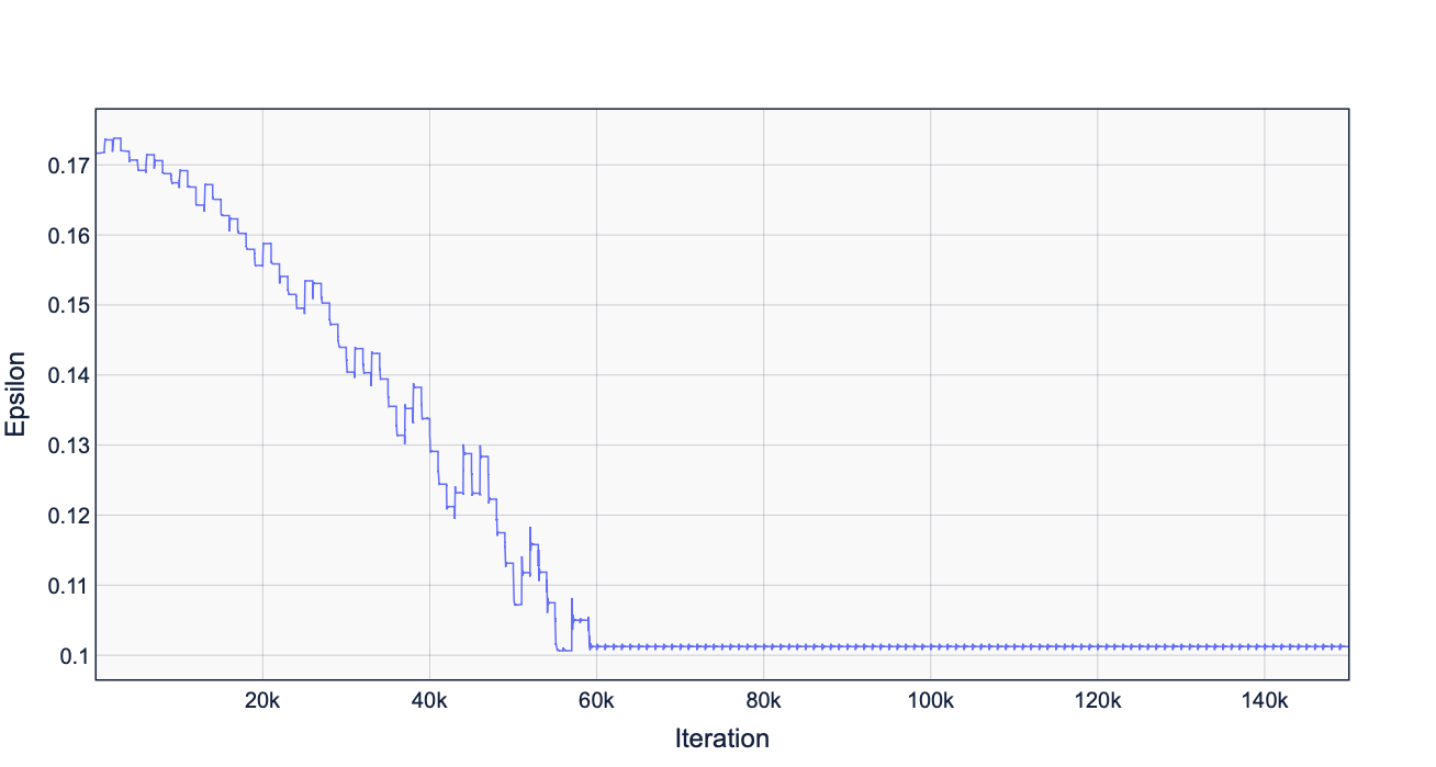
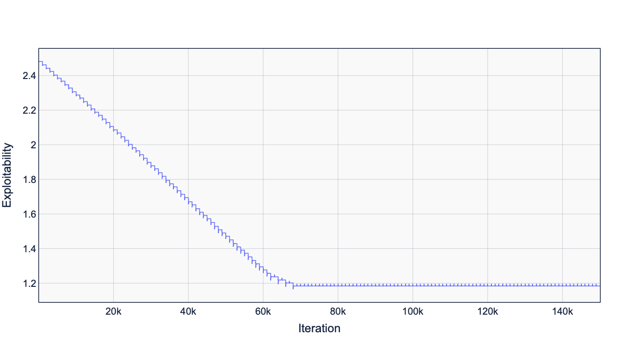
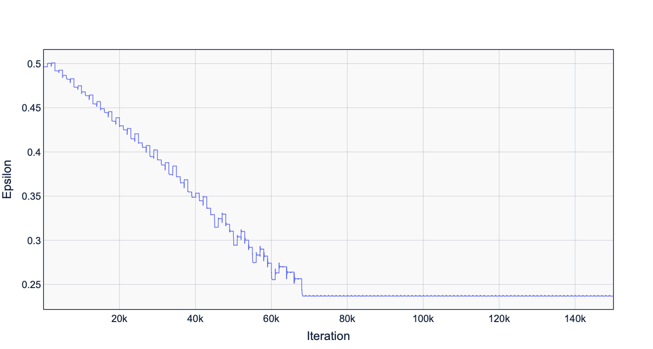
Figure 11. Measures of ‘closeness’ to Nash Equilibrium as the exploration update scheme is applied to the Network Mismatching Game with five agents and (Top) $M=2$ (Bottom) $M=4$. (Left) Distance to NE measured by exploitability (7) of the joint strategy $\mathbf{x}(t)$. (Right) $\epsilon$ as defined by (4). Both metrics decreases as exploration rates are updated until condition (6) fails, after which learning is halted.

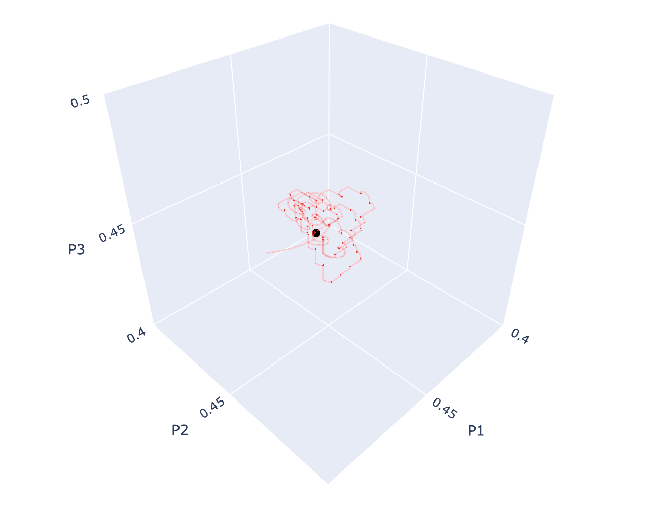
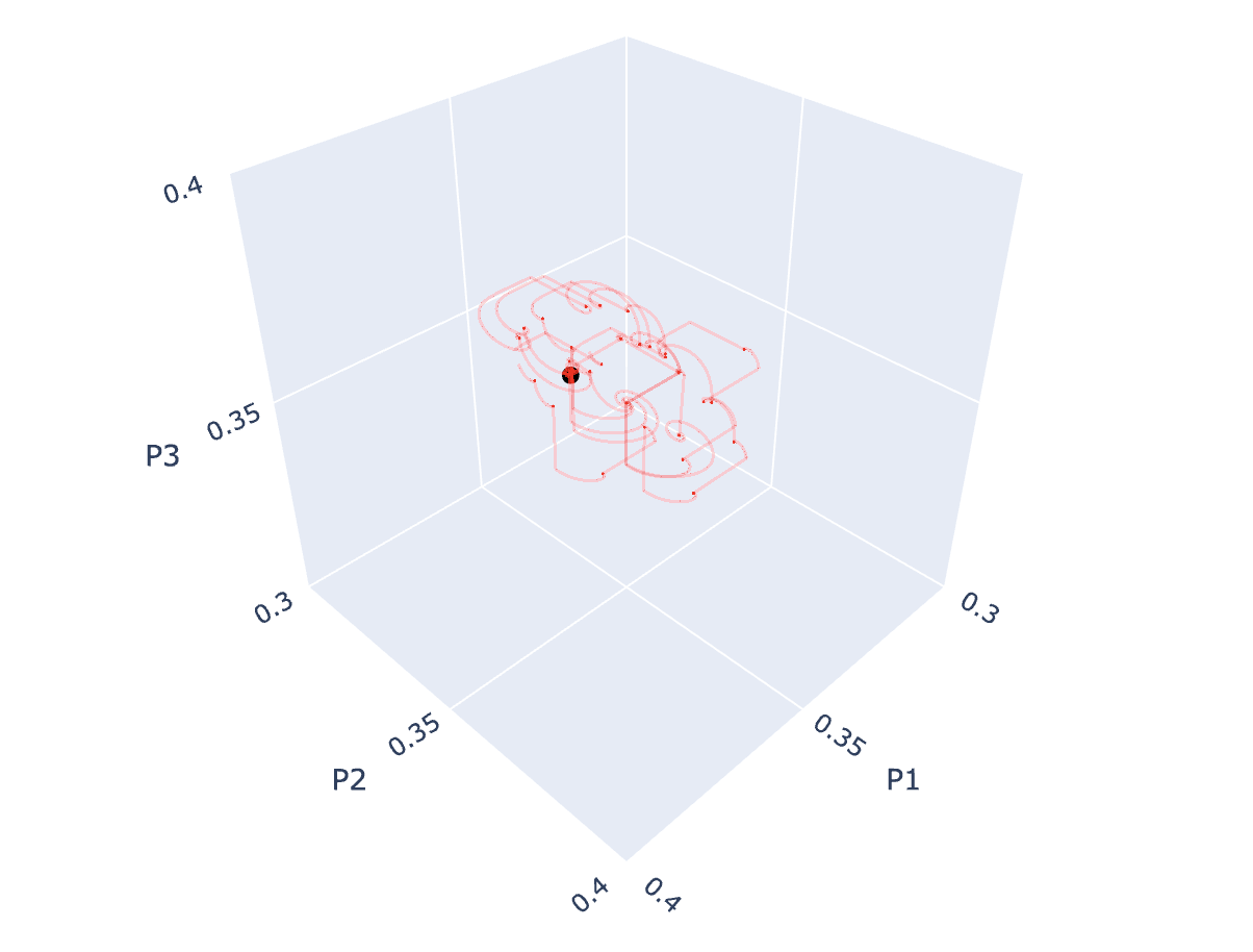
Figure 12. Trajectories of Q-Learning generated as the centralised scheme is applied to (Left) Mismatching Game with $M=2$ (Right) Mismatching Game with $M=4$.

References

- (1)
- Amelina et al. (2015) Natalia Amelina, Alexander Fradkov, Yuming Jiang, and Dimitrios J Vergados. 2015. Approximate Consensus in Stochastic Networks with Application to Load Balancing. IEEE Transactions on Information Theory 61, 4 (9 2015), 1739–1752. https://doi.org/10.1109/TIT.2015.2406323
- Ballester et al. (2006) Coralio Ballester, Antoni Calvó-Armengol, and Yves Zenou. 2006. Who’s Who in Networks. Wanted: The Key Player. Econometrica 74, 5 (2006), 1403–1417. http://www.jstor.org/stable/3805930
- Bielawski et al. (2021) Jakub Bielawski, Thiparat Chotibut, Fryderyk Falniowski, Grzegorz Kosiorowski, Michał Misiurewicz, and Georgios Piliouras. 2021. Follow-the-Regularized-Leader Routes to Chaos in Routing Games. (2 2021). http://arxiv.org/abs/2102.07974
- Bramoullé et al. (2014) Yann Bramoullé, Rachel Kranton, and Martin D’Amours. 2014. Strategic Interaction and Networks. The American Economic Review 104, 3 (2014), 898–930. http://www.jstor.org/stable/42920723
- Camerer et al. (2004) Colin F. Camerer, Teck Hua Ho, and Juin Kuan Chong. 2004. Behavioural game theory: Thinking, learning and teaching. Advances in Understanding Strategic Behaviour: Game Theory, Experiments and Bounded Rationality (1 2004), 120–180. https://doi.org/10.1057/9780230523371{_}8/COVER
- Cheung and Piliouras (2019) Yun Kuen Cheung and Georgios Piliouras. 2019. Vortices Instead of Equilibria in MinMax Optimization: Chaos and Butterfly Effects of Online Learning in Zero-Sum Games. In Proceedings of the Thirty-Second Conference on Learning Theory (Proceedings of Machine Learning Research, Vol. 99), Alina Beygelzimer and Daniel Hsu (Eds.). PMLR, 807–834. https://proceedings.mlr.press/v99/cheung19a.html
- Cheung and Tao (2020) Yun Kuen Cheung and Yixin Tao. 2020. Chaos of Learning Beyond Zero-sum and Coordination via Game Decompositions. (8 2020). http://arxiv.org/abs/2008.00540
- Chotibut et al. (2019a) Thiparat Chotibut, Fryderyk Falniowski, Michał Misiurewicz, and Georgios Piliouras. 2019a. The route to chaos in routing games: Population increase drives period-doubling instability, chaos & inefficiency with Price of Anarchy equal to one. (2019). http://arxiv.org/abs/1906.02486
- Chotibut et al. (2019b) Thiparat Chotibut, Fryderyk Falniowski, Michał Misiurewicz, and Georgios Piliouras. 2019b. The route to chaos in routing games: When is Price of Anarchy too optimistic? (2019). http://arxiv.org/abs/1906.02486
- Cominetti et al. (2010) Roberto Cominetti, Emerson Melo, and Sylvain Sorin. 2010. A payoff-based learning procedure and its application to traffic games. Games and Economic Behavior 70, 1 (2010), 71–83. https://doi.org/10.1016/j.geb.2008.11.012
- Czechowski and Piliouras (2022) Aleksander Czechowski and Georgios Piliouras. 2022. Poincaré-Bendixson Limit Sets in Multi-Agent Learning; Poincaré-Bendixson Limit Sets in Multi-Agent Learning. In International Conference on Autonomous Agents and Multiagent Systems. www.ifaamas.org
- Facchinei and Pang (2004) Francisco Facchinei and Jong Shi Pang. 2004. Finite-Dimensional Variational Inequalities and Complementarity Problems. Finite-Dimensional Variational Inequalities and Complementarity Problems (2004). https://doi.org/10.1007/B97543
- Galla (2011) Tobias Galla. 2011. Cycles of cooperation and defection in imperfect learning. Journal of Statistical Mechanics: Theory and Experiment 2011, 8 (8 2011). https://doi.org/10.1088/1742-5468/2011/08/P08007
- Galla and Farmer (2013) Tobias Galla and J. Doyne Farmer. 2013. Complex dynamics in learning complicated games. Proceedings of the National Academy of Sciences of the United States of America 110, 4 (2013), 1232–1236. https://doi.org/10.1073/pnas.1109672110
- Gemp et al. (2022) Ian Gemp, Rahul Savani, Marc Lanctot, Yoram Bachrach, Thomas Anthony, Richard Everett, Andrea Tacchetti, Tom Eccles, and János Kramár. 2022. Sample-Based Approximation of Nash in Large Many-Player Games via Gradient Descent. In Proceedings of the 21st International Conference on Autonomous Agents and Multiagent Systems (AAMAS ’22). International Foundation for Autonomous Agents and Multiagent Systems, Richland, SC, 507–515.
- Grammatico et al. (2016) Sergio Grammatico, Francesca Parise, Marcello Colombino, and John Lygeros. 2016. Decentralized Convergence to Nash Equilibria in Constrained Deterministic Mean Field Control. IEEE Trans. Automat. Control 61, 11 (11 2016), 3315–3329. https://doi.org/10.1109/TAC.2015.2513368
- Griffin et al. (2022) Christopher Griffin, Justin Semonsen, and Andrew Belmonte. 2022. Generalized Hamiltonian Dynamics and Chaos in Evolutionary Games on Networks. Physica A: Statistical Mechanics and its Applications 597 (7 2022).
- Hadikhanloo et al. (2022) Saeed Hadikhanloo, Rida Laraki, Panayotis Mertikopoulos, and Sylvain Sorin. 2022. Learning in nonatomic games part I Finite action spaces and population games. Journal of Dynamics and Games. 2022 0, 0 (2022), 0. https://doi.org/10.3934/JDG.2022018
- Hamann (2018) Heiko Hamann. 2018. Swarm Robotics: A Formal Approach. Springer International Publishing. https://doi.org/10.1007/978-3-319-74528-2
- Harris (1998) Christopher Harris. 1998. On the Rate of Convergence of Continuous-Time Fictitious Play. Games and Economic Behavior 22, 2 (2 1998), 238–259. https://doi.org/10.1006/game.1997.0582
- Herings and Peeters (2010) P Jean-Jacques Herings and Ronald Peeters. 2010. Homotopy methods to compute equilibria in game theory. Economic Theory 42, 1 (2010), 119–156. https://doi.org/10.1007/s00199-009-0441-5
- Hoang et al. (2018) Quan Hoang, Tu Dinh Nguyen, Trung Le, and Dinh Phung. 2018. MGAN: Training Generative Adversarial Nets with Multiple Generators. In International Conference on Learning Representations.
- Hofbauer and Sigmund (1998) Josef Hofbauer and Karl Sigmund. 1998. Evolutionary Games and Population Dynamics. Cambridge University Press. https://doi.org/10.1017/CBO9781139173179
- Hoorfar and Hassani (2008) Abdolhossein Hoorfar and Mehdi Hassani. 2008. Inequalities on the Lambert W function and hyperpower function. J. Inequal. Pure and Appl. Math 9, 2 (2008), 5–9.
- Hussain et al. (2023a) Aamal Hussain, Francesco Belardinelli, and Georgios Piliouras. 2023a. Beyond Strict Competition: Approximate Convergence of Multi Agent Q-Learning Dynamics. In Proceedings of the Thirty-Second International Joint Conference on Artificial Intelligence (IJCAI-23). https://www.ijcai.org/proceedings/2023/0016.pdf
- Hussain et al. (2023b) Aamal Abbas Hussain, Francesco Belardinelli, and Georgios Piliouras. 2023b. Asymptotic Convergence and Performance of Multi-Agent Q-Learning Dynamics. In Proceedings of the 2023 International Conference on Autonomous Agents and Multiagent Systems (AAMAS ’23). International Foundation for Autonomous Agents and Multiagent Systems, Richland, SC, 1578–1586.
- Imhof et al. (2005) Lorens A. Imhof, Drew Fudenberg, and Martin A. Nowak. 2005. Evolutionary cycles of cooperation and defection. In Proceedings of the National Academy of Sciences of the United States of America. Vol. 102. 10797–10800. https://doi.org/10.1073/pnas.0502589102
- Kadan and Fu (2021) Amit Kadan and Hu Fu. 2021. Exponential Convergence of Gradient Methods in Concave Network Zero-Sum Games. Lecture Notes in Computer Science (including subseries Lecture Notes in Artificial Intelligence and Lecture Notes in Bioinformatics) 12458 LNAI (2021), 19–34. https://doi.org/10.1007/978-3-030-67661-2{_}2/FIGURES/3
- Kianercy and Galstyan (2012) Ardeshir Kianercy and Aram Galstyan. 2012. Dynamics of Boltzmann Q learning in two-player two-action games. Physical Review E - Statistical, Nonlinear, and Soft Matter Physics 85, 4 (4 2012), 041145. https://doi.org/10.1103/PhysRevE.85.041145
- Kleinberg et al. (2011) Robert Kleinberg, Katrina Ligett, Georgios Piliouras, and Eva Tardos. 2011. Beyond the Nash Equilibrium Barrier. Innovations in Computer Science (2011).
- Leonardos and Piliouras (2022) Stefanos Leonardos and Georgios Piliouras. 2022. Exploration-exploitation in multi-agent learning: Catastrophe theory meets game theory. Artificial Intelligence 304 (2022), 103653. https://doi.org/10.1016/j.artint.2021.103653
- Leonardos et al. (2021) Stefanos Leonardos, Georgios Piliouras, and Kelly Spendlove. 2021. Exploration-Exploitation in Multi-Agent Competition: Convergence with Bounded Rationality. Advances in Neural Information Processing Systems 34 (12 2021), 26318–26331.
- LI et al. (2017) Chongxuan LI, Taufik Xu, Jun Zhu, and Bo Zhang. 2017. Triple Generative Adversarial Nets. In Advances in Neural Information Processing Systems, I Guyon, U Von Luxburg, S Bengio, H Wallach, R Fergus, S Vishwanathan, and R Garnett (Eds.), Vol. 30. Curran Associates, Inc. https://proceedings.neurips.cc/paper_files/paper/2017/file/86e78499eeb33fb9cac16b7555b50767-Paper.pdf
- Maynard Smith (1974) J. Maynard Smith. 1974. The theory of games and the evolution of animal conflicts. Journal of Theoretical Biology 47, 1 (9 1974), 209–221. https://doi.org/10.1016/0022-5193(74)90110-6
- McKelvey and Palfrey (1995) Richard D. McKelvey and Thomas R. Palfrey. 1995. Quantal Response Equilibria for Normal Form Games. Games and Economic Behavior 10, 1 (7 1995), 6–38. https://doi.org/10.1006/GAME.1995.1023
- Meiss (2007) James D. Meiss. 2007. Differential Dynamical Systems. Society for Industrial and Applied Mathematics. https://doi.org/10.1137/1.9780898718232
- Melo (2018) Emerson Melo. 2018. A Variational Approach to Network Games. SSRN Electronic Journal (11 2018). https://doi.org/10.2139/SSRN.3143468
- Melo (2021) Emerson Melo. 2021. On the Uniqueness of Quantal Response Equilibria and Its Application to Network Games. SSRN Electronic Journal (6 2021). https://doi.org/10.2139/SSRN.3631575
- Mertikopoulos et al. (2018) Panayotis Mertikopoulos, Christos Papadimitriou, and Georgios Piliouras. 2018. Cycles in adversarial regularized learning. Proceedings (2018), 2703–2717. https://doi.org/10.1137/1.9781611975031.172
- Mertikopoulos and Sandholm (2016) Panayotis Mertikopoulos and William H. Sandholm. 2016. Learning in Games via Reinforcement and Regularization. https://doi.org/10.1287/moor.2016.0778 41, 4 (8 2016), 1297–1324. https://doi.org/10.1287/MOOR.2016.0778
- Metrick and Polak (1994) Andrew I Metrick and Ben Polak. 1994. Fictitious play in 2 • 2 games: a geometric proof of convergence*. Econ. Theory 4 (1994), 923–933.
- Mukhopadhyay and Chakraborty (2020) Archan Mukhopadhyay and Sagar Chakraborty. 2020. Deciphering chaos in evolutionary games. Chaos 30, 12 (12 2020), 121104. https://doi.org/10.1063/5.0029480
- Pandit et al. (2018) Varun Pandit, Archan Mukhopadhyay, and Sagar Chakraborty. 2018. Weight of fitness deviation governs strict physical chaos in replicator dynamics. Chaos: An Interdisciplinary Journal of Nonlinear Science 28, 3 (3 2018), 033104. https://doi.org/10.1063/1.5011955
- Pangallo et al. (2019) Marco Pangallo, Torsten Heinrich, and J. Doyne Farmer. 2019. Best reply structure and equilibrium convergence in generic games. Science Advances 5, 2 (2 2019). https://doi.org/10.1126/SCIADV.AAT1328/SUPPL{_}FILE/AAT1328{_}SM.PDF
- Pangallo et al. (2022) Marco Pangallo, James B.T. Sanders, Tobias Galla, and J. Doyne Farmer. 2022. Towards a taxonomy of learning dynamics in 2 × 2 games. Games and Economic Behavior 132 (3 2022), 1–21. https://doi.org/10.1016/J.GEB.2021.11.015
- Parise et al. (2020) Francesca Parise, Sergio Grammatico, Basilio Gentile, and John Lygeros. 2020. Distributed convergence to Nash equilibria in network and average aggregative games. Automatica 117 (2020), 108959. https://doi.org/10.1016/j.automatica.2020.108959
- Parise and Ozdaglar (2019) Francesca Parise and Asuman Ozdaglar. 2019. A variational inequality framework for network games: Existence, uniqueness, convergence and sensitivity analysis. Games and Economic Behavior 114 (3 2019), 47–82. https://doi.org/10.1016/j.geb.2018.11.012
- Perolat et al. (2020) Julien Perolat, Remi Munos, Jean Baptiste Lespiau, Shayegan Omidshafiei, Mark Rowland, Pedro Ortega, Neil Burch, Thomas Anthony, David Balduzzi, Bart de Vylder, Georgios Piliouras, Marc Lanctot, and Karl Tuyls. 2020. From poincaré recurrence to convergence in imperfect information games: finding equilibrium via regularization. Technical Report.
- Perrin et al. (2020) Sarah Perrin, Julien Perolat, Mathieu Lauriere, Matthieu Geist, Romuald Elie, and Olivier Pietquin. 2020. Fictitious Play for Mean Field Games: Continuous Time Analysis and Applications. In Advances in Neural Information Processing Systems, H Larochelle, M Ranzato, R Hadsell, M F Balcan, and H Lin (Eds.), Vol. 33. Curran Associates, Inc., 13199–13213. https://proceedings.neurips.cc/paper/2020/file/995ca733e3657ff9f5f3c823d73371e1-Paper.pdf
- Rosen (1965) J Rosen. 1965. Existence and Uniqueness of Equilibrium Points for Concave N-Person Games. Econometrica 33, 3 (1965).
- Sanders et al. (2018) James B T Sanders, J Doyne Farmer, and Tobias Galla. 2018. The prevalence of chaotic dynamics in games with many players. Scientific Reports 8, 1 (2018), 4902. https://doi.org/10.1038/s41598-018-22013-5
- Sato et al. (2004) Yuzuru Sato, Eizo Akiyama, and James P Crutchfield. 2004. Stability and diversity in collective adaptation. Physica D: Nonlinear Phenomena 210 (2004), 21–57.
- Sato et al. (2002) Yuzuru Sato, Eizo Akiyama, and J. Doyne Farmer. 2002. Chaos in learning a simple two-person game. Proceedings of the National Academy of Sciences of the United States of America 99, 7 (4 2002), 4748–4751. https://doi.org/10.1073/pnas.032086299
- Sato and Crutchfield (2003) Yuzuru Sato and James P. Crutchfield. 2003. Coupled replicator equations for the dynamics of learning in multiagent systems. Physical Review E 67, 1 (1 2003), 015206. https://doi.org/10.1103/PhysRevE.67.015206
- Schwartz (2014) Howard M. Schwartz. 2014. Multi-Agent Machine Learning: A Reinforcement Approach. Wiley. 1–242 pages. https://doi.org/10.1002/9781118884614
- Shapley (2016) L. S. Shapley. 2016. Some Topics in Two-Person Games. In Advances in Game Theory. (AM-52). Princeton University Press, 1–28. https://doi.org/10.1515/9781400882014-002
- Shokri and Kebriaei (2020) Mohammad Shokri and Hamed Kebriaei. 2020. Leader-Follower Network Aggregative Game with Stochastic Agents’ Communication and Activeness. IEEE Trans. Automat. Control 65, 12 (12 2020), 5496–5502. https://doi.org/10.1109/TAC.2020.2973807
- Sorin and Wan (2016) Sylvain Sorin and Cheng Wan. 2016. Finite composite games: Equilibria and dynamics. Journal of Dynamics and Games 3, 1 (2016), 101–120.
- Sutton and Barto (2018) R Sutton and A Barto. 2018. Reinforcement Learning: An Introduction. MIT Press. http://incompleteideas.net/book/the-book-2nd.html
- Szabó and Fáth (2007) György Szabó and Gábor Fáth. 2007. Evolutionary games on graphs. Physics Reports 446, 4 (2007), 97–216. https://doi.org/10.1016/j.physrep.2007.04.004
- Tatarenko and Kamgarpour (2019) Tatiana Tatarenko and Maryam Kamgarpour. 2019. Learning Nash Equilibria in Monotone Games. Proceedings of the IEEE Conference on Decision and Control 2019-December (12 2019), 3104–3109. https://doi.org/10.1109/CDC40024.2019.9029659
- Turocy (2005) Theodore L Turocy. 2005. A dynamic homotopy interpretation of the logistic quantal response equilibrium correspondence. Games and Economic Behavior 51, 2 (2005), 243–263. https://doi.org/10.1016/j.geb.2004.04.003
- Tuyls (2023) Karl Tuyls. 2023. Multiagent Learning: From Fundamentals to Foundation Models. In Proceedings of the 2023 International Conference on Autonomous Agents and Multiagent Systems (AAMAS ’23). International Foundation for Autonomous Agents and Multiagent Systems, Richland, SC, 1.
- Tuyls et al. (2006) Karl Tuyls, Pieter Jan T Hoen, and Bram Vanschoenwinkel. 2006. An Evolutionary Dynamical Analysis of Multi-Agent Learning in Iterated Games. Autonomous Agents and Multi-Agent Systems 12, 1 (2006), 115–153. https://doi.org/10.1007/s10458-005-3783-9
- van Strien and Sparrow (2011) Sebastian van Strien and Colin Sparrow. 2011. Fictitious play in 3×3 games: Chaos and dithering behaviour. Games and Economic Behavior 73, 1 (2011), 262–286. https://doi.org/10.1016/j.geb.2010.12.004
- Vlatakis-Gkaragkounis et al. (2020) Emmanouil-Vasileios Vlatakis-Gkaragkounis, Lampros Flokas, Thanasis Lianeas, Panayotis Mertikopoulos, and Georgios Piliouras. 2020. No-Regret Learning and Mixed Nash Equilibria: They Do Not Mix. Advances in Neural Information Processing Systems 33 (2020), 1380–1391.