Fractal ground state of ion chains in periodic potentials

Abstract

Trapped ions in a periodic potential are a paradigm of a frustrated Wigner crystal. The dynamics is captured by a long-range Frenkel-Kontorova model. The classical ground state can be mapped to the one of an antiferromagnetic spin chain with long-range interactions in a magnetic field, whose strength is determined by the mismatch between chain’s and substrate lattice’s periodicity. The mapping is exact when the substrate potential is a piecewise harmonic potential and holds for any two-body interaction decaying as $1/r^{\alpha}$ with the distance $r$. The ground state is a devil’s staircase of regular, periodic structures as a function of the mismatch, whose range of stability depends also on the coefficient $\alpha$. While the staircase is well defined in the thermodynamic limit for $\alpha>1$, for Coulomb interactions, $\alpha=1$, it disappears and the sliding-to-pinned transitions becomes crossovers. However, due to the logarithmic convergence to the thermodynamic limit characteristic of the Coulomb potential, the staircase is found for any finite number of ions. We discuss the experimental parameters as well as the features that allow one to observe and reveal our predictions in experimental platforms. These dynamics are a showcase of the versatility of trapped ion platforms for exploring the interplay between frustration and interactions.

I Introduction

Chains of laser-cooled ions in linear Paul traps are paradigmatic realizations of a harmonic crystal in one dimension Dubin and O’Neil (1999). In these systems, order emerges from the interplay between the Coulomb repulsion and the trapping potential. Even in one dimension, the long-range nature of Coulomb interactions warrants diagonal (quasi) long-range order, and any finite chain is effectively a one-dimensional Wigner crystal Schulz (1993). At the typical temperatures reached by laser cooling the ions vibrate harmonically at the crystal equilibrium position and their motion is described by an elastic crystal with power-law coupling Morigi and Fishman (2004). The experimental capability to image and monitor the individual ions makes ion chains a prominent platform for studying structural phase transitions Birkl et al. (1992); Raizen et al. (1992); Dubin (1993); Fishman et al. (2008) and the static and dynamic properties of crystal dislocations Ulm et al. (2013); Pyka et al. (2013); Mielenz et al. (2013); Ejtemaee and Haljan (2013); Brox et al. (2017a); Kiethe et al. (2017, 2018); Gangloff et al. (2020). The progress in cooling and trapping Eschner et al. (2003) paves the way for investigating these dynamics deep in the quantum regime Shimshoni et al. (2011); Zhang et al. (2023); Bonetti et al. (2021); Timm et al. (2021); Vanossi et al. (2013); Zanca et al. (2018).

Interfacing ion chains with optical lattices, as illustrated in Fig. 1, implements a simulator of nanofriction Vanossi et al. (2013). In fact, the Hamiltonian can be reduced to an extended Frenkel-Kontorova (FK) model García-Mata, I. et al. (2007); Pruttivarasin et al. (2011); Cetina et al. (2013); Cormick and Morigi (2013). The FK model describes the interaction of an elastic crystal with an underlying periodic substrate in one dimension Braun and Kivshar (2004). Frustration emerges from the mismatch between the periodicity of the elastic crystal and of the substrate. The ground-state phase diagram of the FK model has been extensively studied for nearest-neighbour interactions: When the corresponding ratio is an incommensurate number, at zero temperature the FK model reproduces the essential features of the stick-slip motion characteristic of static friction, with a continuous transition from sliding to pinning at finite lattice depths. As a function of the mismatch, the ground state is non-analytic and has a form of a devil’s staircase, whose steps correspond to the regime of stability of a commensurate structure, i.e.  a periodic structure pinned by the lattice Aubry and Le Daeron (1983). The transition to a sliding phase is characterized by the proliferation of kinks, namely, of local distributions of excess particles (or holes) in the substrate potential Braun and Kivshar (2004). Realizations with trapped ions observed several features of this dynamics: Stick-slip motion has been reported in experiments with few ions Gangloff et al. (2015); Bylinskii et al. (2015, 2016), pinning by an external lattice has been observed Linnet et al. (2012), the onset of the Aubry transition has been measured in an implementation simulating a deformable substrate Kiethe et al. (2017), and the kinks density has been revealed in small chains as a function of the mismatch Gangloff et al. (2020).

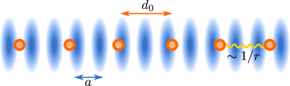
Figure 1: Illustration of a trapped-ion realization of the Frenkel-Kontorova model. A chain of cold ions (orange circles) at uniform distance $d_{0}$ minimizing the Coulomb repulsion. The ions are interacting with the standing wave of a laser field (blue shades), forming a periodic potential with periodicity $a$. For $d_{0}\gg a$ the ions’ motion about the equilibrium positions is described by their harmonic vibrations about the equilibrium configuration and the dynamics is captured by a Frenkel-Kontorova model with long-range elastic forces.

These results show the versatility of trapped ion platforms as quantum simulators. Recent progress in cooling large ion chains Lechner et al. (2016); Feng et al. (2020) and loading ions in optical lattices Schmidt et al. (2018); Hoenig et al. (2023) pave the way towards studying kinks dynamics and their mutual interactions, thus shedding light into the interplay between geometric frustration and quantum fluctuations. In this regime, long-range forces, such as the Coulomb repulsion, qualitatively modify the kinks and the nature of their interactions Pokrovsky and Virosztek (1983). A systematic study can be performed in the continuum limit, when the substrate potential is a small perturbation to the chain’s interaction and the kinks are Sine-Gordon solitons for nearest-neighbor interactions Frank et al. (1949). Then, the long-range interactions modify the Sine-Gordon equation introducing an integral term Landa et al. (2020) and the long-range Sine-Gordon model can be mapped to an extended massive (1+1) Thirring Hamiltonian, where the solitons are charged positive energy excitations over a Dirac sea Menu et al. (2023). This theory has a predictive power for ion chains provided the average interparticle distance is orders of magnitude larger than the potential periodicity, allowing one to discard the discrete nature of the charge density distribution. The theory does not capture the opposite limit, where either the number of ions is limited to few dozens Bylinskii et al. (2016); Kiethe et al. (2018); Gangloff et al. (2020) and/or the depth of the substrate potentials localizes the kinks at chain sizes of a few ions as in Refs. Landa et al. (2013); Partner et al. (2013). In some treatments the discrete nature of the charge distribution can be theoretically described as corrections to the continuum limit Willis et al. (1986); Braun et al. (1990); Chelpanova et al. (2024), leading to effective soliton-phonon collisions Willis et al. (1986).

In the present work, we choose a different approach and start from a discrete distribution of interacting particles. Due to the long-range interactions, the ground state emerging from the competition of interactions and substrate potential cannot be found by means of the ingenious dynamical map of Ref. Aubry and Le Daeron (1983). We instead implement the method of Hubbard Hubbard (1978), and map the ground state configuration of the long-range, Coulomb Frenkel-Kontorova model to the one of an antiferromagnetic spin chain in the presence of a transverse field. The mapping is exact for a periodic substrate composed of piecewise harmonic oscillators Beyeler et al. (1980), illustrated in the upper panel of Fig. 2, and is amenable to analytical solutions. Despite the theoretical abstraction, we show that this mapping sheds light on the properties of realistic substrate potentials, such as an optical lattice.

The presentation of our study is organised as follows. In Sec. II it is shown that the ground state and low-energy excitations of a Wigner crystal of ions in a linear Paul trap are described by a Frenkel-Kontorova (FK) model where the oscillators of the elastic crystal interact via the long-range Coulomb interactions. This Section reviews the arguments presented in Refs. García-Mata, I. et al. (2007); Pruttivarasin et al. (2011); Cormick and Morigi (2013) and sets the stage for our analysis. The ground state is determined in Sec. III within a mean-field approach, which discards the kinetic energy. Here, we assume a specific function of the periodic substrate and map the continuous-variable problem onto an antiferromagnetic Ising model with long-range interactions and in the presence of a magnetic field, as illustrated in the lower panel of Fig. 2. Our mapping extends the study of Ref. Beyeler et al. (1980) to a Wigner crystal and allows us to show that the ground state is a devil’s staircase as a function of the mismatch between the lattice periodicity and the characteristic interparticle distance. It allows us, moreover, to determine the interval of stability of the individual commensurate structures as a function of the temperature. In Sec. IV we determine the low-energy excitations of an ion chain in a periodic potential across the Aubry transition and identify the experimental signatures. We then discuss the order of magnitude of quantum fluctuations by means of a semiclassical ansatz. The conclusions are drawn in Sec. V, where we provide an outlook of the directions of studies that our study opens towards the systematic characterization of the interplay between long-range interactions and geometric frustration with cold atoms platforms.

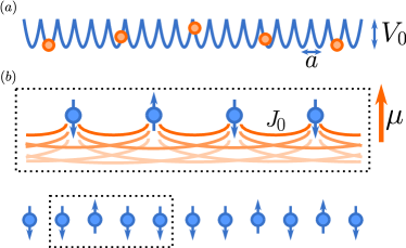
Figure 2: (a) Frenkel-Kontorova model where the periodic substrate potential is a piecewise parabolic function, Eq. (9) (in blue). The orange circles represent the interacting particles forming a chain. (b) The number of vacant sites $h_{j}$ between neighbouring particles is mapped onto a spin whose orientation depends on the value of $h_{j}$, as shown in Sec. IV. In the effective model, the depth of the substrate potential $V_{0}$ determines the short-range behavior of the antiferromagnetic spin-spin coupling $J_{0}$ while the mismatch is a magnetic field $\mu$. The central panel is a magnified fragment of the spin larger chain indicated by the dotted box. The power-law decay of the interactions is indicated by the gradual attenuation of the connecting edges.

II Chain of interacting particles in a periodic potential

This section reviews the basic assumptions and the steps that connect the Hamiltonian of a one-dimensional Wigner crystal of ions in a periodic potential with a Frenkel-Kontorova model of oscillators interacting via power-law decaying forces. We then generally discuss the geometric properties of the ground state using the characterization of Hubbard Hubbard (1978) and introduce the quantities that will be important for performing the mapping in Sec. III. We refer the interested reader to Refs. García-Mata, I. et al. (2007); Pruttivarasin et al. (2011), where it was proposed to study the sliding-to-pinning transition using Wigner crystals of trapped ions in optical lattices.

II.1 Extended Frenkel-Kontorova model

We consider $N$ particles of mass $M$ in one dimension, ordered along the $x$–axis. Let $x_{j}$ be the particles’ positions, with $j=1,\ldots,N$, such that $x_{j}<x_{i}$ for $j<i$. We denote by $L$ the chain’s length and assume periodic boundary conditions. The particles interact via the repulsive two-body potential $W(x)$, that decays algebraically with the distance $x$ as

$$W(x)=W_{0}/x^{\alpha}\,$$

with $W_{0}>0$. In this section we keep the power law exponent $\alpha$ generic, restricting to values $\alpha\geq 1$, hence including also the Coulomb interaction.

The overall potential energy includes a periodic substrate potential $V_{s}(x)$ and takes the form

$$V=\dfrac{W_{0}}{2}\sum_{i,j}\dfrac{1}{|x_{i}-x_{j}|^{\alpha}}+\sum_{j}V_{s}(x_{j}),$$ (1)

where we assume periodic boundary conditions and that $V_{s}(x)$ has periodicity $a$, $V_{s}(x+a)=V_{s}(x)$. For later convenience, we write the substrate potential as

$$V_{s}(x)=V_{0}f(x),$$

where $V_{0}\in\mathbb{R}^{+}$ determines the depth of the potential and $f(x)$ is a dimensionless periodic function with unit amplitude.

In order to link the model of Eq. (1) with the paradigmatic Frenkel-Kontorova model, we assume that the particles are localized about the equilibrium positions of the potential $W(x)$, and perform a Taylor expansion of the interaction $W(x)$ about the classical equilibrium positions $x_{j}^{(0)}$ assuming that the average interparticle distance $d_{0}=L/N$ is much larger than the lattice periodicity $a$, thus $x_{j}^{(0)}=jd_{0}$. We denote by $u_{j}$ the local displacement of the particles $u_{j}$ from $x_{j}^{(0)}$, such that $x_{j}=x_{j}^{(0)}+u_{j}$. In second order in the expansion in the small parameter $u_{j}/d$ the potential reads:

$$V\simeq W^{(0)}+V_{0}\sum_{j}{f(x_{j})}+\dfrac{1}{2}\sum_{j}\sum_{n>0}{\dfrac{K}{n^{\alpha+2}}(u_{j+n}-u_{j})^{2}}\,,$$ (2)

where $W^{(0)}$ is the interaction potential at the equilibrium positions,

$$W^{(0)}=\frac{W_{0}}{2}\sum_{i,j}\dfrac{1}{|x_{i}^{(0)}-x_{j}^{(0)}|^{\alpha}}\,,$$

and $K$ is the spring stiffness,

$$K=\frac{\alpha(\alpha+1)W_{0}}{d_{0}^{\alpha+2}}\,.$$

Equation (2) corresponds to the potential of the Frenkel-Kontorova model with power-law elastic interactions.

Some words of caution about this treatment shall be spent. In fact, the validity of the Taylor expansion requires that the classical ground state is stable against fluctuations. In one dimension this is not verified for interactions with exponent $\alpha>1$: In that case the treatment here presented is valid only for sufficiently small chains, while for long chains the ground state is captured by a Luttinger model, see Ref. Dalmonte et al. (2010). The Coulomb chain, $\alpha=1$, is a special case due to the non-additivity of the energy, that leads to the slow decay of two-point density correlations with distance Schulz (1993); Morigi and Fishman (2004). As a consequence, for any finite size the Coulomb chain exhibits long-range order even at zero temperatures.

II.2 Potential of the vacant sites

Hereafter, we will assume that at most one particle is assigned to each lattice site. In order to distinguish classical configurations, we will introduce the notation of Ref. Beyeler et al. (1980): Let $h_{n}$ be the number of vacant sites between two subsequent particles of the chain. The sequence $\{h_{1},\dots,h_{N}\}$ fully characterizes a classical equilibrium configuration. The potential energy of Eq. (2) can be expressed in terms of the sequence of vacant sites, $\{h_{1},\dots,h_{N}\}$, via the equivalent reformulation of the position variables

$$x_{j}=a\sum_{i=1}^{j-1}{(h_{i}+1)}+\delta x_{j},$$ (3)

where now $\delta x_{j}$ is the displacement of the particle with respect to the closest substrate-potential well. Using Eq. (3) and that $f(x_{j})=f(\delta x_{j})$, we cast the potential, Eq. (2), in the form:

$$V \simeq V^{(0)}+V_{0}\sum_{j}{f(\delta x_{j})}+\dfrac{K}{2}\sum_{j}\sum_{n>0}{\dfrac{1}{n^{\alpha+2}}(\delta x_{j+n}-\delta x_{j})^{2}}+aK\sum_{j}\sum_{n>0}{\dfrac{1}{n^{\alpha+2}}(\delta x_{j+n}-\delta x_{j})(h^{(n)}_{j}-n\langle h\rangle)}$$

$$+a^{2}\dfrac{K}{2}\sum_{j}\sum_{n>0}{\dfrac{1}{n^{\alpha+2}}(h^{(n)}_{j}-n\langle h\rangle)^{2}},$$ (4)

where $V^{(0)}$ is the potential in zeroth order in the expansion in $\delta x_{j}$, and we have introduced the notation

$$h^{(n)}_{j}=\sum_{i=0}^{n-1}{h_{j+i}}\,.$$ (5)

Equation (II.2) is the starting point for performing a mapping to a potential of interacting spins. A crucial part of this mapping consists of eliminating the displacement variables $\delta x_{j}$ and rewriting the potential energy only in terms of the vacant-site variables $h_{n}$, which in turn will be mapped onto spins.

II.3 Equilibrium configurations

The ground states configurations of potential (II.2) are determined by the competition of the power-law interaction and the periodic substrate potential. Moreover, they shall satisfy the additional constraint of periodic boundary conditions. We first note that the length $L$ of the chain shall be an integer multiple $N_{s}$ of the substrate periodicity $a$: $L=N_{s}a$. This establishes a relation between the average interparticle distance, $d_{0}=L/N$, and the lattice periodicity $a$, given by $Nd_{0}=N_{s}a$. From these quantities we find the mean number of particles per lattice site, which we denote by $\rho$:

$$\rho=\dfrac{N}{N_{s}}=\dfrac{a}{d_{0}}\,.$$ (6)

We can further link the density with the the average number of empty sites, $\langle h\rangle=\sum_{j}h_{j}/N$, by observing that the sum of vacant sites shall fulfil the relation

$$\sum_{j}h_{j}=N_{s}-N\,.$$ (7)

Dividing both sides by $N$, we link the average number of empty sites with the density of charges:

$$\langle h\rangle=\dfrac{1}{\rho}-1\,.$$ (8)

Due to the periodic boundary conditions, the structures emerging from the competition between the substrate potential and the two-body interactions are necessarily periodic. True incommensurate structures will then exist in the strict thermodynamic limit. For finite-size chains we will denote a structure as incommensurate when the following condition occurs. Let $P$ be the period characterizing the structure: $P=L/M$ with $M$, a natural number such that $M\geq 1$. A structure will be commensurate when $M>1$. On the contrary, incommensurate configurations are characterized by $P=L$, namely, the period is the full length of the chain. See also Ref. Roux et al. (2008) for a related discussion.

In what follows we will consider the case $\rho<1$. The Taylor expansion of Eq. (2), in particular, requires that the particles displacement is of the order of the lattice periodicity and thus is valid for densities $\rho\ll 1$.

III Ground state of the piece-wise parabolic potential

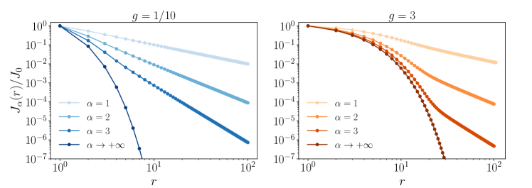
Figure 3: Coefficients of the interacting potential for the vacant sites. The coefficient $J_{\alpha}(r)$, Eq. (LABEL:eq:J:0) are displayed as a function of the distance $r$ (in units of $a$) for a deep ($g=1/10$) and a shallow ($g=3$) substrate lattice. The colors refer to different values of the power-law exponent $\alpha$, see legenda. The logarithmic scale emphasizes the two-fold behavior of the coefficients, which at short distances decay exponentially while at long distances decay algebraically as $1/r^{\alpha}$ for finite exponents $\alpha$. The nearest-neighbor case ($\alpha\to\infty$) is solely characterized by the exponential decay.

We now show that the model of Eq. (II.2) can be mapped to a long-range antiferromagnetic Ising model in the presence of a magnetic field, as illustrated in Fig. 2. The classical ground state of this model is a devil’s staircase as a function of the density $\rho$ Bak and Bruinsma (1982). The mapping we perform is exact when the periodic substrate potential is a sequence of piecewise-truncated parabolas of the form

$$f(\delta x)=\dfrac{4}{a^{2}}\delta x^{2},$$ (9)

for $|\delta x|\leq a/2$, see Fig. 2 (a). This functional behavior was assumed by Frenkel and Kontorova in their original model Frenkel and Kontorova (1938), and has been used in several analyses (see, e.g., Aubry (1983); Beyeler et al. (1980); Krajewski and Müser (2005)).

III.1 Mean-field configuration in Fourier representation

The mapping is performed by first eliminating the displacement $\delta x_{j}$ from the potential of Eq. (II.2) and expressing the potential itself as a function of the segments of vacancies, $h_{j}$. For this purpose, we introduce the Fourier components for the variables of interest

$$Q_{q} =\dfrac{1}{\sqrt{N}}\sum_{j}{e^{-iqja}\delta x_{j}},$$ (10a)

$$\zeta_{q} =\dfrac{1}{\sqrt{N}}\sum_{j}{e^{-iqja}(h_{j}-\langle h\rangle)}\,,$$ (10b)

where $q$ is the wave number in the Brillouin zone of the lattice. For convenience, we also introduce the Fourier components of the sequences of vacancies, $h^{(n)}_{j}$, namely

$$\zeta^{(n)}_{q} =\dfrac{1}{\sqrt{N}}\sum_{j}{e^{-iqja}(h^{(n)}_{j}-n\langle h\rangle)}\,.$$

Using Eq. (5), this expression takes the compact form:

$$\zeta^{(n)}_{q} =\zeta_{q}\sum_{j=0}^{n-1}{e^{iqja}}=\dfrac{1-e^{iqna}}{1-e^{iqa}}\zeta_{q}\,.$$ (11)

On the basis of these definitions, the potential energy can be rewritten in terms of the Fourier components.

$$V =V^{(0)}+\dfrac{8V_{0}}{a^{2}}\sum_{q>0}{Q_{q}Q_{-q}(1+g\phi_{\alpha}(q))}$$

$$+a\dfrac{8V_{0}}{a^{2}}\sum_{q>0}\left({Q_{q}\zeta_{-q}\dfrac{g\phi_{\alpha}(q)}{e^{-iqa}-1}+\mathrm{c.c.}}\right)$$

$$+a^{2}\dfrac{8V_{0}}{a^{2}}\sum_{q>0}{\zeta_{q}\zeta_{-q}\dfrac{g\phi_{\alpha}(q)}{|e^{iqa}-1|^{2}}},$$ (12)

where the long-range nature of the interactions is now encoded in the function $\phi(q)$, defined such that

$$\phi_{\alpha}(q)=\sum_{n>0}{\dfrac{|1-e^{iqna}|^{2}}{n^{\alpha+2}}}\,.$$ (13)

Now, the dimensionless coefficient

$$g=\frac{Ka^{2}}{8V_{0}}$$ (14)

quantifies the competition between the elastic properties of the chain and the interaction with the substrate.

For nearest-neighbor interactions ($\alpha\to\infty$) the parameter $g$ controls the transition from sliding, where solitons proliferate ($g\gg 1$), to pinning ($g\ll 1$), where the formation of the soliton is energetically costly.

Our interest lies in determining how the periodic potential stabilizes a new ordering of the chain of particles. Equilibrium requires the condition $\frac{\partial V}{\partial Q_{q}}=0$ for all values of the wave number $q$. This condition leads to a linear relation between the displacements and the sequences of vacant sites

$$Q_{q}=-a\,g\dfrac{\phi_{\alpha}(q)}{1+g\phi_{\alpha}(q)}\left(\dfrac{1}{e^{iqa}-1}\right)\zeta_{q}\,.$$ (15)

We note that the coefficient $g$ is inversely proportional to the square of the mass of the sine-Gordon kink $M_{\rm SG}$ Braun and Kivshar (2004); Landa et al. (2020):

$$M^{2}_{\rm SG}=\dfrac{\pi^{2}}{3g}\,.$$ (16)

III.2 The potential for the vacant sites

By means of Eq. (15), we can recast the expression of the potential energy in terms of the Fourier components of the vacant sites only. In real space, the potential for the vacant sites takes the form:

$$V=V^{0}+\sum_{\ell}\sum_{r}J_{\alpha}(r)(h_{\ell}-\langle h\rangle)(h_{\ell+r}-\langle h\rangle)\,,$$ (17)

with the interaction coefficient:

$$J_{\alpha}(r) = \frac{4V_{0}}{N}\sum_{q}\cos(qra)\frac{g}{1+g\phi_{\alpha}(q)}\,\frac{\phi_{\alpha}(q)}{\phi_{\infty}(q)}\,,$$

where $\phi_{\infty}(q)=\lim_{\alpha\to\infty}\phi_{\alpha}(q)=|e^{iqa}-1|^{2}$.

It is instructive to analyse the generic behavior of the coefficients $J_{\alpha}(r)$ as a function of $r$ for finite power-law exponents $\alpha$, see Fig. 3. We first note that $|\phi_{\alpha}(q)|\leq 2\zeta(\alpha+2)$, with $\zeta(\alpha)$ the Riemann zeta function. By means of an analytic continuation, it becomes visible that the pole of the function $\mathcal{F}_{\alpha}(q)=1+g\phi_{\alpha}(q)$ determines an exponentially decaying behavior with a characteristic length that is monotonically increasing with $g$, see Appendix A. For nearest-neighbor interactions ($\alpha\to+\infty$), the coefficient decays exponentially with a damping length monotonically increasing with $g$. Instead, for finite values of $\alpha$, we observe a two-fold behaviour of $J_{\alpha}(r)$: at short distances the coefficient decays exponentially, whereas at long distances $|r|\gg a$ the coefficient exhibits a power-law tail solely determined by the long-range interactions. In Appendix A we show that the power-law tail takes the form

$$J_{\alpha}(r)\simeq\dfrac{Ka^{2}}{2}\dfrac{\Gamma(\alpha)}{\Gamma(\alpha+2)}\dfrac{1}{|r|^{\alpha}}\,,$$ (19)

which is independent of $g$. At large distances, thus, the coefficient describes a power-law repulsion at the same exponent $\alpha$ of the interaction. This is in agreement with the general considerations of Refs. Pokrovsky and Virosztek (1983); Braun et al. (1990); Landa et al. (2020). The short-distance and large-distance behavior of the coefficient $J_{\alpha}(r)$ is visible in Fig. 3 for deep ($g=1/10$) and shallow lattices ($g=3$) for representative values of the exponent $\alpha$.

III.3 The dislocation

By transforming back into the space variables, we obtain the equilibrium positions of the ions as a function of the empty sequences. For $g\gg 1$ the displacements take the form (see Appendix B:)

$$\delta x_{j} \approx a\frac{g}{\alpha+1}\sum_{r>0}\frac{1}{r^{\alpha+1}}(h_{j+r}-h_{j-r})\,.$$ (20)

This expression provides the shape of the dislocation. We introduce the phase field $\theta_{j}/2\pi$:

$$\theta_{j}=\frac{2\pi}{a}\left(x_{j}-ja\left(\dfrac{d_{0}}{a}-\delta\right)\right),$$ (21)

The phase field is displayed on Fig. 4 for two values of the coefficient $g$. Each step is a dislocation inside the ion chain. Decreasing the value of $g$, thus increasing the amplitude of the substrate potential, leads to increasingly sharper jumps in the shape of the phason, as the ions become pinned to the local minima of the substrate potential.

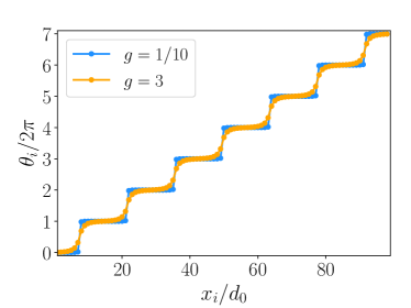
Figure 4: Dislocations for different lattice depths. A phason $\theta_{i}/2\pi$, corresponding to the in-well displacement $\delta x_{j}/a$, is displayed as a function of the ion position $x_{i}$. Calculations are performed for $N=99$ ions and density $\rho=99/700$ in the case of a deep (blue) and shallow (orange) substrate potential.

III.4 A long-range antiferromagnetic spin model

The segments $h_{j}$ in Eq. (17) can be interpreted as interacting spins Beyeler et al. (1980). For this purpose, it is now useful to recall that the segments of vacant sites $h_{j}$ can only be integer numbers. In a commensurate structure where the equilibrium interparticle distance is $\bar{d}_{0}=(n_{0}+1)a$, the number of vacancies is uniform and equal to $h_{j}=n_{0}$. A discommensurate structure, instead, is characterized by an average interparticle distance

$$d_{0}=\bar{d}_{0}+\delta a\,,$$ (22)

where the parameter $\delta$ determines the discommensuration (or mismatch), $0<\delta<1$. In the ground state the segments rearrange such that $h_{j}$ can either be $n_{0}$ or $n_{0}+1$, satisfying the constraint imposed by Eq. (7), see Refs. Hubbard (1978); Bak and Bruinsma (1982). Since the number of vacant sites can only take two values, we will treat them as classical spins $S_{j}=\pm 1$ where

$$S_{j}=2(h_{j}-n_{0})-1\,.$$

Thus, $S_{j}=1$ when $h_{j}=n_{0}+1$ and $S_{j}=-1$ when $h_{j}=n_{0}$. We use that $\langle h\rangle=n_{0}+\delta$ and rewrite the potential energy as a spin Hamiltonian of the form

$${\mathcal{H}}=\dfrac{1}{4}\sum_{i\neq j}{J(i-j)(S_{i}+1)(S_{j}+1)}-\mu\sum_{i}{S_{i}}\,,$$ (23)

where $J(r)=J_{\alpha}(r)$. This Hamiltonian describes an Ising antiferromagnetic chain in the magnetic field of strength

$$\mu=2\delta\sum_{r>0}J(r)\,.$$ (24)

The magnetic field, in turn, is proportional to the discommensuration and tends to align the spin, competing with the antiferromagnetic order imposed by the interactions.

The Hamiltonian in Eq. (23) is given apart for a constant energy offset $E_{0}$, which is positive and depends on the discommensuration: $E_{0}=2N\delta(\delta-1/2)\sum_{r>0}J(r)$.

III.5 Devil’s staircase

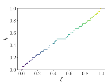
Figure 5: Devil’s staircase of commensurate structures as a function of the mismatch. The plot shows the magnetization, here represented in terms of the ratio $\overline{h}=m/n$ of up-oriented spins, as a function of the magnetic field, here given by the discommensuration $\delta$. The staircase has been numerically determined using the method of Ref. Koziol et al. (2023) for a chain of $N=200$ ions ($\alpha=1$) and $g\ll 1$. The displayed plateaus correspond here to the ratios $m/n$ with $n\leq 20$.

The phase diagram of the spin model of Eq. (23) entails the so-called Aubry transition as well as the commensurate-incommensurate transition Bak (1982). At both transitions the ground state becomes non-analytic. The fractal nature of the ground state becomes visible when considering the so-called magnetization $M$ as a function of the magnetic field. $M$ is given by

$$M=\sum S_{j}/N=2\bar{h}-1\,,$$ (25)

with $\bar{h}=\langle h\rangle-n_{0}$ the effective discommensuration. In the absence of the substrate potential, $\bar{h}=\delta$, and the magnetization is proportional to the magnetic field. At finite substrate depths instead, $\bar{h}$ exhibits a devil staircase as a function of $\delta$ as shown in Fig. 5. The phase diagram of some commensurate phases in the $g-\delta$ plane is displayed in Fig. 6(a) for the Wigner crystal. One observes that the size decreases as the lattice depth decreases (corresponding to increasing $g$).

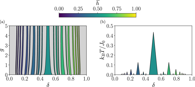
Figure 6: (a) Magnetization, $\overline{h}=m/n$, as a function of the discommensuration $\delta$ and of the ratio $g$ between the stiffness and the potential depth. Colored areas represent plateaus corresponding to ratios $\overline{h}$ with $n\leq 8$. In the grey areas the plateaus of the staircase are below the chosen resolution. (b) The magnetization $\overline{h}=m/n$ as a function of the discommensuration $\delta$ and of the temperature $T$ for $g\ll 1$. Colored areas represent plateaus corresponding to ratios $\overline{h}$ with $n\leq 8$. White areas correspond to a paramagnetic, disordered phase. All calculations are performed for a chain of $N=50$ ions interacting via Coulomb repulsion ($\alpha=1$).

III.6 Thermodynamic limit and phase transitions

The size of the steps of the devil’s staircase of Fig. 5 agrees with an analytical expression obtained by means of sum rules for generic, convex interactions Hubbard (1978); Bak and Bruinsma (1982). For a magnetization with $\bar{h}=m/n$ ( $m$ and $n$ natural numbers and prime to each other) the interval of stability is given by

$$\Delta\mu\left[\dfrac{m}{n}\right]=\sum_{j=1}^{N}{nj\left[J(jn-1)+J(jn+1)-2J(jn)\right]}\,,$$ (26)

This analytical expression provides the boundaries of the stability of classical commensurate structures in the $g-\delta$ plane, and represents the energy gap for flipping a spin in the commensurate phase. It is thus the energy for generating a kink. When the gap vanishes, flipping a spin (generating a dislocation) becomes energetically favorable and kinks proliferate. The gap vanishes at the critical value $g_{c}(\delta)$ at fixed discommensuration $\delta$. This is the critical value of the Aubry transition separating a sliding (gapless) from a pinned (gapped) phase. At fixed $g$, it gives the critical value $\delta_{c}(g)$ at which the commensurate-incommensurate transition occurs. These values can be analytically determined in the thermodynamic limit, letting $N\to\infty$. By means of a proper rescaling (Kac’s rescaling) Campa et al. (2009); Defenu et al. (2019), the critical values $g_{c}$ and $\delta_{c}$ tend to a finite value in the thermodynamic limit for $\alpha>1$. For $\alpha=1$, instead, they vanish, and the phase is always incommensurate in the thermodynamic limit. This behavior is a consequence of the non-additive nature of the energy for Coulomb interactions in one dimension. It is not removed by Kac’s scaling. Kac’s scaling, in fact, re-establishes the extensivity of the energy by renormalizing the mass as $Q^{2}\to Q^{2}/\ln N$ Morigi and Fishman (2004); Landa et al. (2020). Then, $g\propto 1/\ln N$ and it vanishes in the thermodynamic limit. The interaction coefficients scale as $1/\ln N$ and correspondingly the size of the plateaus $\Delta\mu\sim 1/\ln N$, and thus $\Delta\mu\to 0$ for $N\to\infty$. This behavior is in agreement with the prediction that for Coulomb interactions the fractal dimension is unity Bruinsma and Bak (1983). It is a manifestation of the long-range nature of the Coulomb interaction which tends to prevail over the order imposed by the external lattice. As a consequence, Aubry transition and commensurate-incommensurate transitions are crossovers for finite $N$. Nevertheless, given the extremely slow growth of $\ln N$ with $N$, these transitions can be experimentally revealed, provided that the temperature of the chain is sufficiently low, as we discuss in the next section.

III.7 Thermal effects

With an argument based on the scaling of entropy in the free energy, Peierls showed that in one dimension thermal fluctuations prevent the emergence of magnetic order Peierls (1936). This observation holds in the thermodynamic limit and for systems with additive energy. For finite system, there is a temperature $T(N)$ above which the commensurate structure becomes unstable. The temperature $T(N)$ decreases with $N$, and vanishes in the thermodynamic limit.

We estimate $T(N)$ using a semiclassical model, where we calculate the change of free energy by creating a defect in the commensurate structure as $\Delta F=\Delta E-T\Delta S$, where $\Delta E$ is the change in energy and $\Delta S$ the one in entropy. By means of the mapping to the antiferromagnetic spin model, then $\Delta E=\Delta\mu$ of Eq. (26). The change in entropy can be determined within the spin model. For a $n$-partite ordered magnetic phase, the total entropy takes the form Erba et al. (2021)

$$S=\dfrac{Nk_{B}}{n}\left[n\ln 2-\sum_{\sigma=\pm}\sum_{r=1}^{n}{\dfrac{1+\sigma m_{r}}{2}\ln(1+\sigma m_{r})}\right],$$ (27)

where the set $\{m_{r}\}$ corresponds to the magnetization of each of the $n$ sublattices. For a perfectly ordered phase ($m_{r}=\pm 1$), the entropy cost of flipping a single spin (so for a variation of magnetization $dm_{r}=n/N$) scales like in the thermodynamic limit as $S\sim k_{B}\ln(N/n)/2$. Therefore, the free energy cost of flipping a spin starting from the magnetically ordered (commensurate) phase at a given value of $\overline{h}$ is given by

$$\Delta F(\overline{h})=\Delta\mu[\overline{h}]-k_{B}T\dfrac{n}{4}\ln\left(\dfrac{N}{n}\right),$$ (28)

and it is stable for $\Delta F>0$. The quantity $\Delta F(\overline{h})$ provides the size of the plateaus at finite temperatures. Interestingly, also the entropy change depends on $n$ and increases with $n$. This expression also shows that the temperature below which the commensurate structure $\overline{h}$ is stable, scales as

$$k_{B}T(N)\sim\frac{4\Delta_{\mu}(\overline{h})}{n}\frac{1}{\ln(N/n)}\,.$$

On the basis of this expression, it is possible to establish a phase diagram describing the ordering of the spin chain with regard to thermal fluctuations. Figure 6(b) displays the phase diagram at constant $g\ll 1$ in the $\delta-T$ plane. We observe the progressive shrinking of the plateaus of the staircase as the thermal fluctuations become increasingly prominent. These results also allow to estimate the temperature below which one can expect to observe an incomplete devil’s staircase in a realistic trapped-ion experiments. For an experimental set-up similar to the one realized in Bylinskii et al. (2016), one can expect to observe plateaus below $T\lesssim 1\,\mathrm{mK}$.

IV Phonon spectra and semiclassical limit

In this section we analyse the low-energy excitations of a Coulomb chain across the transition assuming the temperature is below $T(N)$. In our analysis the spectrum consists of the linear excitations of the classical ground state. We consider an experimentally relevant configuration, where the substrate potential is sinusoidal. Correspondingly, the function in Eq. (1) reads

$$f(x)=1-\cos\left(\dfrac{2\pi}{a}x\right)\,.$$ (29)

This function is continuous and permits us to perform the Taylor expansion about the equilibrium positions for any value of $g$. The corresponding kink, in the continuum limit, is a Sine-Gordon soliton with long-range tails Landa et al. (2020).

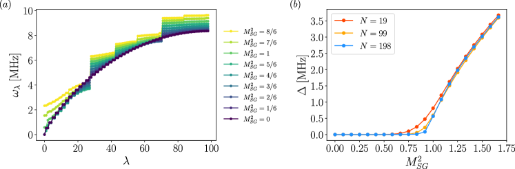
Figure 7: Vibrational spectrum. (a) Eigenfrequencies $\omega_{\lambda}$ for an ion chain and several values of the parameter $M_{SG}$. Here, $\lambda$ labels the eigenmodes for increasing frequency. Here, the density is $\rho=99/721$ and the particles interact via the Coulomb repulsion ($\alpha=1$). (b) Spectral gap as a function of $M_{SG}$ for a fixed value of the density $\rho$ and $N=19,99,198$. The calculations are performed using the parameters of Cetina et al. (2013), taking ${}^{174}\mathrm{Yb}^{+}$ ions with interparticle distance $d_{0}=6\mu\mathrm{m}$ and lattice periodicity $a=185\mathrm{nm}$.

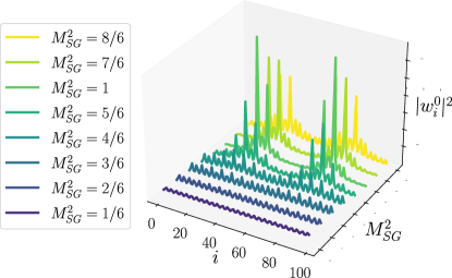
Figure 8: Spatial form of the lowest-energy mode $|w^{0}_{i}|^{2}$ as a function of the mass of the soliton $M_{SG}$. The considered chain contains $N=99$ ions at a density $\rho=99/721$. Calculations are performed for ${}^{174}\mathrm{Yb}^{+}$ ions with the characteristic lengths of the experiment described in Cetina et al. (2013).

IV.1 Ground state configuration

The equilibrium positions minimize the potential (1) and are determined numerically via a gradient-descent algorithm. We denote by $\{\bar{x}_{i}^{(0)}\}$ the ensemble of solutions. Defining the local displacement with respect to these equilibrium position as $x_{i}=\bar{x}_{i}^{(0)}+\bar{u}_{i}$, the potential energy is expanded up to the second order in the displacement:

$$H\simeq\dfrac{1}{2M}\sum_{i}{p^{2}_{i}}+\bar{V}^{(0)}+\dfrac{1}{2}\sum_{i,j}{\bar{u}_{i}\mathcal{K}_{ij}\bar{u}_{j}}+\mathcal{O}(u^{3})\,,$$ (30)

where now $\bar{V}^{(0)}$ is the potential at the equilibrium positions $\{\bar{x}_{i}^{(0)}\}$ and $\mathcal{K}_{ij}$ are the elements of the symmetric stiffness matrix for the equilibrium configuration of the whole potential. The diagonal elements read

$$\mathcal{K}_{ii} =\left(\dfrac{2\pi}{a}\right)^{2}V_{0}\cos\left(\dfrac{2\pi}{a}\bar{x}_{i}^{(0)}\right)+\sum_{k\neq i}{\dfrac{2\alpha(\alpha+1)W_{0}}{|\bar{x}_{i}^{(0)}-\bar{x}_{k}^{(0)}|^{\alpha+2}}}\,,$$ (31)

while the off-diagonal elements take the form:

$$\mathcal{K}_{ij} =-\dfrac{\alpha(\alpha+1)W_{0}}{|\bar{x}_{i}^{(0)}-\bar{x}_{j}^{(0)}|^{\alpha+2}}\,.$$ (32)

IV.2 Vibrational spectrum

The vibrational spectrum is found by diagonalizing the quadratic potential with the usual procedure, consisting in identifying the corresponding orthogonal matrix $O\in SO(N)$, such that $O^{-1}=O^{T}$. In the quadratic form, the Hamiltonian $H$ reads

$$H=V^{(0)}+\sum_{\lambda}{\left[\frac{1}{2M}p_{\lambda}^{2}+\frac{1}{2}M\omega^{2}_{\lambda}u^{2}_{\lambda}\right]}\,.$$

The eigenvalues given by $M\omega^{2}_{\lambda}$ are positive when the equilibrium configuration is stable. The frequencies $\omega_{\lambda}$ give the dispersion relation, where $\lambda$ labels the eigenmode and is not the quasi-momentum of the lattice since the potential is generally aperiodic. Figure 7(a) displays the vibrational spectrum of the ion chain for different values of $M_{SG}$ across the Aubry transition. An increase of the strength of the substrate potential $V_{0}$ (and therefore of $M_{SG}$) leads to the opening of gaps in the spectrum. On the other hand, the large-wavelength properties are relatively unperturbed up to a critical value where a gap opens at $k\to 0$.

Figure 7(b) shows the value of lowest eigenfrequency, $\Delta=\min_{\lambda}\omega_{\lambda}$, as a function of $M_{SG}$ and for a fixed value of the density. This quantity is an order parameter, that signals the transition between the incommensurate phase, which is self-similar, and the commensurate phase, where the array is pinned by the substrate lattice. One observes a sudden change from a vanishing gap to a finite one starting from a threshold value of $M^{2}_{SG}\sim 0.9$. The opening of the gap heralds the transition toward a pinned phase for which translation invariance is no longer spontaneously broken.

Given that the Hamiltonian is generally not symmetric under discrete translations, the eigenmodes $\lambda$ are not phonon modes. The dependence of the lowest frequency ones is shown in Fig. 8 as a function of the position and the mass of the soliton. This figure shows that, when increasing the substrate potential, and consequently the mass of the soliton, the lowest-frequency mode departs increasingly from a uniformly distributed form to more complex ones displaying several localized excitations. This structure indicates that the mode of lowest frequency does not correspond to a wave vector $k=0$.

IV.3 Quantum fluctuations

The mean-field model is amenable to a semiclassical analysis, which can allow us to estimate its stability against quantum fluctuations. This is done according to this phenomenological ansatz: We quantize the fluctuations about the classical ground state and estimate the maximal size at $T=0$. The commensurate phase is stable when the wave packets of all ions are localized within the corresponding well of the substrate potential. We note that this ansatz is plausible away from the transition point.

We now spell out the criterion. We denote by $\delta x_{i}$ the displacement with respect to the closest potential minimum, such that $|\delta x_{i}|\leq a/2$. The displacement can be separated into the sum of two contributions: the mean-field displacement $\delta x_{i}^{(0)}$, that determines the equilibrium position of the ion within the well, and the spatial extension of the wavepacket $\delta u$, which we define as

$$\delta u=\max_{i=1,\ldots,N}\sqrt{|\delta x_{i}^{2}|-\delta x_{i}^{(0)\,2}}\,.$$ (33)

We determine $\delta u$ as follows. We first quantize the displacements, $\hat{u}_{\lambda}=\sqrt{u_{0\lambda}/2}(\hat{a}_{\lambda}+\hat{a}^{\dagger}_{\lambda})$ and the canonically conjugated momentum $\hat{p}_{\lambda}=-i\sqrt{(\hbar/2u_{0,\lambda}}(\hat{a}_{\lambda}-\hat{a}^{\dagger}_{\lambda})$, with $u_{0,\lambda}=\hbar/M\omega_{\lambda}$ and $[\hat{a}_{\lambda},\hat{a}^{\dagger}_{\lambda^{\prime}}]=\delta_{\lambda,\lambda^{\prime}}$. The Hamiltonian for the quantum fluctuations is the sum of quantum harmonic oscillators, $H_{q}=\sum_{\lambda}\hbar\omega_{\lambda}(\hat{a}^{\dagger}_{\lambda}\hat{a}_{\lambda}+1/2)$.

The quantum fluctuations can be related to the phonon modes via the relation $u_{i}=\sum_{\lambda}w_{i}^{\lambda}u_{\lambda}$, where $w_{i}^{\lambda}$ are the elements of the orthogonal matrix $O$ diagonalizing the quadratic Hamiltonian. Assuming that the system is at temperature $T=0$, then all phonon modes are in their ground state, and $\langle u_{i}^{2}\rangle=\sum_{\lambda}{\frac{\hbar}{2M\omega_{\lambda}}(w^{\lambda}_{i})^{2}}$. The total displacement is shown in Fig. 9 as a function of the mean-field displacement. The dashed line represents the value $|\delta x_{i}|=a/2$, where the quantum fluctuations become relevant and the mean-field treatment fails. For $g<g_{c}$ the quantum corrections are essentially negligible and the displacement with respect to the local minima of the substrate potential remain below the threshold. As $g$ increases towards the critical value, one can observe an increasing role of the quantum fluctuations. This graphic analysis permits us to estimate the value of $g$ at which the semiclassical regime becomes invalid.

IV.4 Experimental realization

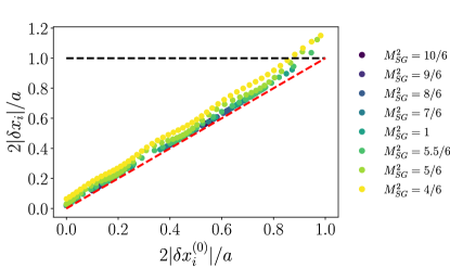
Figure 9: Local displacement of the particles as a function of the mean-field displacement, plotted for a fixed density $\rho=99/721$ and several values of the soliton mass $M^{2}_{SG}$. The black dashed line represents the threshold value of $|\delta x_{i}|=a/2$, while the red dashed line accounts for the classical behaviour. The parameters are the same as in Fig. 7.

The theory developed here is motivated by existing experiments which have measured the Aubry transition in ion chains Kiethe et al. (2017); Bylinskii et al. (2016). Their feasibility has been extensively discussed in previous literature García-Mata, I. et al. (2007); Pruttivarasin et al. (2011); Cetina et al. (2013); Cormick and Morigi (2013). In this section we focus on the core assumptions of our work. Throughout this work we have assumed that -in the absence of the optical lattice- the ions are equidistant. In a linear Paul trap, this is fulfilled at the chain center Morigi and Fishman (2004); Kiethe et al. (2018). It is also possible to shape the macrocopic trap potential to approximate a box potential using several electrodes, resulting in a near-homogeneous ion spacing over an extended region. An interesting alternative is offered by ring trap geometries Li et al. (2017). Here, a periodic substrate along the ring could be created by a second ion species with different mass Landa et al. (2014); Fogarty et al. (2013). Observing reasonably sharp transition requires chains with several tens of ions.

Kinks and dislocations can be imaged Pyka et al. (2013); Ulm et al. (2013); Mielenz et al. (2013) and spectroscopically resolved Brox et al. (2017b); Kiethe et al. (2018). This permits to determine the behavior at the Aubry transition as well as at the commensurate-incommensurate transition. Features of the devil’s staircase are visible as long as thermal excitations are smaller than the gap Shimshoni et al. (2011); Kiethe et al. (2021). Our study permits to identify the temperatures required: Using the parameters of Ref. Bylinskii et al. (2016), for a chain of 100 ions ¹⁷¹Yb⁺ with interparticle distance $d_{0}=6\mu\mathrm{m}$ and lattice periodicity $a=185\mathrm{nm}$, steps of the devil’s staircase with magnetization $k=m/n$ will be measurable for temperatures $T\lesssim 1\,\mathrm{mK}/n$.

Quantum effects at the transition manifest as tunnelling of the solitons, and tend to stabilize the commensurate phase. Within our mean-field approach, we have included them as a perturbation and have analysed the corresponding qualitative features numerically. Other studies followed a different ansatz where the soliton tunnels across the Peierls-Nabarro potential Timm et al. (2021). The full quantum dynamics has been numerically studied for few ions in Bonetti et al. (2021). Finally, in a recent work we derived a mapping valid deep in the incommensurate phase Menu et al. (2023). All these considerations lead us to predict that quantum effects at the Aubry and at the commensurate-incommensurate transition should be visible, provided the chain is cooled to temperatures below mK.

V Conclusions

We have determined the classical ground state of a Frenkel-Kontorova model with long-range interactions. When the substrate potential is given by piecewise harmonic oscillators, the long-range Frenkel-Kontorova model can be exactly mapped onto a chain of spin with long-range antiferromagnetic interactions and an external magnetic field. The structure of the coefficients allows us to shed light on the behavior at the commensurate-incommensurate transition and at the Aubry transition. While for power-law interactions scaling as $1/r^{\alpha}$ and $\alpha>1$ the transitions are well defined also in the thermodynamic limit, for Coulomb interactions, $\alpha=1$, they become a crossover. We have discussed the features signalling the onset of the transitions in an experiment with trapped ions. Importantly, we predict that this transition can still be observed in realistic finite-size experiments, given our analysis of the devil’s staircase as a function of the temperature and of the number of ions.

In terms of the theoretical model, our study is complementary to existing works and approaches Timm et al. (2021); Bonetti et al. (2021); Menu et al. (2023). The mapping, in fact, allows us to take into full account the discrete nature of the lattice and to assess its role on transitions that are typically characterized in the continuum limit. The mapping to the model by Ref. Bak and Bruinsma (1982), moreover, opens interesting perspectives for studying topological features, characteristic of the fractional quantum Hall effects in ion chains Rotondo et al. (2016).

Finally, our predictions have been derived for a generic power-law exponent, and are in principle applicable to other systems, such as chains of Rydberg atoms in tweezers arrays Barredo et al. (2016); Endres et al. (2016) or dipoles tightly bound in optically lattices Lahaye et al. (2009); Baranov (2008). While a Luttinger liquid description in these cases is more appropriate Dalmonte et al. (2010), yet our approach shall allow one to capture finite size effects and the role of discreteness in these dynamics.

Our study contributes to clarify the role of long-range, non-additive interactions on the stability of structures that are commensurate with the external substrate and to identify the regime of stability as a function of the physical parameters. Moreover, it sets a semi-analytic benchmark for numerical investigations of geometric frustration in Coulomb systems. Future studies will focus on the effect of deformable substrate potentials, as realised in Refs. Kiethe et al. (2017, 2018) with two ion chains in a linear Paul trap and in Ref. Lauprêtre et al. (2019) by trapping ions in the optical lattice of a high-finesse cavity (see Ref. Cormick and Morigi (2013); Fogarty et al. (2015) for the theoretical predictions in the strong-coupling limit.

Our results support the present atom-based quantum technology platforms as versatile laboratories to probe condensed-matter and high-energy physics hypothesis.

Appendix A Determination of the coefficients $J_{\alpha}(r)$

We here analyse the behavior of the coefficient $J_{\alpha}(r)$ with the distance using the continuum limit of the sum on the right-hand side of Eq. (LABEL:eq:J:0) and performing an analytic continuation. Note that the integral shares several analogies with the integrals performed in Refs. Defenu et al. (2019); Jäger et al. (2020) for chains with power-law decaying interactions, and arguments applied in those works can be also applied to this case. For convenience, we first define the dimensionless function $B_{\alpha}(r)=J_{\alpha}(r)/(4V_{0})$. In the continuum limit, it is an integral over the Brillouin zone:

$$B_{\alpha}(r)\approx\lim_{\eta\to 0^{+}}\frac{1}{2\pi}\int_{\eta}^{2\pi-\eta}{\rm d}q\,{\rm e}^{{\rm i}qra}{\mathcal{M}}_{\alpha}(q)$$ (34)

with

$${\mathcal{M}}_{\alpha}(q)=\frac{1}{2{\mathcal{F}}_{\alpha}(q)}\frac{\phi_{\alpha}(q)}{\phi_{\infty}(q)}\,.$$ (35)

where we have introduced the function

$${\mathcal{F}}_{\alpha}(q)=1/g+\phi_{\alpha}(q)\,.$$ (36)

It is useful to rewrite the function $\phi_{\alpha}(q)$, Eq. (13) as

$$\phi_{\alpha}(q)=2\zeta(\alpha+2)-{\rm Li}_{\alpha+2}({\rm e}^{{\rm i}qa})-{\rm Li}_{\alpha+2}({\rm e}^{-{\rm i}qa})\,,$$ (37)

and ${\rm Li}_{\gamma}(z)=\sum_{n=1}^{\infty}z^{n}/n^{\gamma}$ the polylogarithm Abramowitz and Stegun (1964), while $\zeta(\gamma)=\sum_{n=1}^{\infty}1/n^{\gamma}=\mathrm{Li}_{\gamma}(1)$ stands for the Riemann $\zeta$-function. We also note that in the limit $q\to 0$ the function $\lim_{q\to 0}{\mathcal{M}}_{\alpha}(q)=g\zeta(\alpha)/2$ for all values of $\alpha\geq 1$.

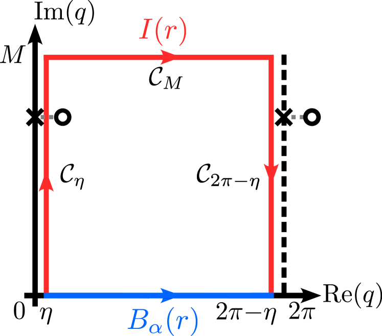
Figure 10: Sketch of the contour integration in (39). Here, the blue line indicates the integration path $\mathcal{C}(y)=y$ along the real axis ($y\in[\eta,2\pi-\eta]$). The red line shows the contour $\mathcal{C}_{\eta}(y)=\eta+iy$ with $y\in[0,M]$, $\mathcal{C}_{M}(y)=y+iM$ with $y\in[\eta,2\pi-\eta]$, and $\mathcal{C}_{2\pi-\eta}(y)=2\pi-\eta+i(M-y)$ with $y\in[0,M]$. Black crosses mark the positions of the displaced poles (black circles) in the limit $\epsilon\to 0+$.

We identify the contour in the complex plane illustrated on Fig. 10. It consists in a contribution along a segment (in blue) of the real axis, integrating between $[\eta,2\pi-\eta]$. It accounts for the quantity $B_{\alpha}(r)$ defined in Eq. (34). The path in red is segmented into three contributions: $\mathcal{C}_{\eta}$ obtained by integrating along the path $z=\eta+iy$, with $y\in[0,M]$, $\mathcal{C}_{M}$ obtained by integrating along the path $z=y+iM$, with $y\in[\eta,2\pi-\eta]$, and $\mathcal{C}_{2\pi-\eta}$ obtained by integrating along the path $z=2\pi-\eta+i(M-y)$, with $y\in[0,M]$. Summing these three integrals yields the contribution $I(r)$. We also notice that in the limit $\eta\to 0^{+}$ the contour intersects with poles located in $z=iq_{0}$ and $z=iq_{0}+2\pi$. This pathological case can however be solved by introducing a shift of the poles by a factor $\epsilon$. As a result, we need to include contributions coming from the pole contained within the contour, namely $z=iq_{0}$.

Using the residue theorem, we rewrite Eq. (34) as the sum of the integral along the contour, $I(r)$, and of the residues it contains, $R(r)$, as it follows

$$B_{\alpha}(r)=R(r)+I(r)\,.$$ (38)

The integral is taken along the contour illustrated in Fig. 10 and reads

$$I(r)=\lim_{\eta\rightarrow 0^{+}}\left[\int_{\mathcal{C}_{\eta}}+\int_{\mathcal{C}_{2\pi-\eta}}+\int_{\mathcal{C}_{M}}\right]dq\,\frac{e^{i|r|q}}{2\pi}{\mathcal{M}}_{\alpha}(q)\,,$$ (39)

The summation over the residues in Eq. (38) goes over the complex numbers $q_{0}$ with ${0\leq\mathrm{Re}(q_{0})<2\pi}$ and ${\mathrm{Im}(r_{0})>0}$ for which $\mathrm{Res}[e^{rq}{\mathcal{M}}(q),q_{0}]$ does not vanish and reads

$$R(r)=i\mathrm{Res}\big{[}e^{i|r|q}{\mathcal{M}}_{\alpha}(q),iq_{0}\big{]}$$ (40)

Below we extend the treatment of Ref. Jäger et al. (2020) to this case and argue that the residues contribute to $B_{\alpha}(r)$ with an exponential decay (see Eq. (44)), while the integral term is different from zero for $\alpha$ finite. In this case its contribution is an algebraic decay with $\alpha$ (see Eq. (48)). In particular, we show that it also holds for $\alpha=1$.

A.1 Exponential decay

For $\alpha>1$ we observe that the only values where $\mathrm{Res}[e^{irq}{\mathcal{M}}_{\alpha}(q),s]$ does not vanish are the zeros of $\mathcal{F}_{\alpha}(q)$, defined in Eq. (36). Therefore we search for the values $s$ such that $\mathcal{F}_{\alpha}(s)=0$. Within the area of the contour ${\mathcal{M}}(q)$ is a meromorphic function and we can take its Laurent series about the root $s$ of $\mathcal{F}_{\alpha}(q)$:

$${\mathcal{M}}_{\alpha}(q)=\sum_{\ell=-\infty}^{\infty}a_{\ell}(s)(q-s)^{\ell}\,,$$ (41)

where the $a_{\ell}$ are the coefficients. Moreover, since ${\mathcal{M}}_{\alpha}(q)$ is meromorphic there exists a finite and positive index $L_{s}$ such that $a_{\ell}(s)=0$ for $\ell<-L_{s}$. This index determines the order of the pole of ${\mathcal{M}}_{\alpha}(q)$ at $s$.

Using Eq. (41) the residues at $s$ can be expressed as

$$\mathrm{Res}\big{[}e^{i|r|q}{\mathcal{M}}_{\alpha}(q),q_{0}\big{]}=e^{i|r|s}P_{s}(r)\,,$$ (42)

where $P_{s}(r)$ is a polynomial in $r$ which depends on the coefficients of the Laurent expansion as

$$P_{s}(r)=\sum_{\ell=0}^{L_{s}-1}\frac{[i|r|]^{\ell}}{\ell!}a_{-1-\ell}(s),$$ (43)

using the expansion of $e^{i|r|(q-s)}$ close to $s$. Since all poles are isolated, then the behavior of Eq. (42) in the bulk is dominated by the residue at the point $s^{\prime}$ with the smallest imaginary part, namely ${\rm Im}(s^{\prime})=\xi$ is such that ${\xi\leq{\rm Im}(s)}$ for all $s$. We distinguish two cases, when $\xi>0$ and when instead $\xi=0$. For $\xi>0$ then for $r\gg 1$ the sum over the residues Eq. (42) behaves as

$$R(r)\sim e^{-\xi|r|}\tilde{P}_{s^{\prime}}(r)\,,$$ (44)

where $\tilde{P}_{s^{\prime}}(r)=iP_{s^{\prime}}(r)e^{i|r|{\rm Re}(s^{\prime})}$. If $s^{\prime}$ is a pole of order one, then the polynomial $P_{s^{\prime}}(r)$ is simply a constant independent on $r$.

The residues are simply found for the case $\alpha\to\infty$, where the interaction is nearest-neighbour. Then $\mathcal{F}_{\infty}(q)$ has two poles, $q_{\pm}=\pm i\ln(\epsilon+\sqrt{\epsilon^{2}-1})=\pm iq_{0}$, where for convenience we have introduced $\epsilon=1+1/(2g)$. Only the pole $q_{+}$ is within the contour, and we obtain

$$R(r)=\frac{V_{0}}{2}\,\left(g\frac{{\rm e}^{-q_{0}|r|}}{\sqrt{4g+1}}\right)\,.$$ (45)

This expression agrees with Equation (3.23) of Ref. Beyeler et al. (1980) (note that their coefficient $g$ is our $g$ divided by 2).

When $\xi=0$, a pole of $F_{\alpha}(q)$ lies on the real axis. We note that it can occur only for $g\to\infty$, which is outside of the validity of our model. For $\alpha=1$, instead, there is no simple pole.

A.2 Power-law tails

We will now extract the behavior of the integrals in Eq. (39). For this purpose we use that $\int_{\mathcal{C}_{M}}dqe^{i|r|q}{\mathcal{M}_{\alpha}}(q)$ vanishes in the limit $M\to\infty$. In this limit the integral to solve is

$$I(r) =-\frac{1}{\pi}\int_{0}^{+\infty}e^{-y|r|}{\rm Im}({\mathcal{M}}_{\alpha}(iy))\mathrm{d}y\,.$$ (46)

Here, ${\mathcal{M}}_{\alpha}(q)$ is given in Eq. (35), and its imaginary part specifically reads:

$$\mathrm{Im}({\mathcal{M}}_{\alpha}(iy))=-\frac{1}{g}\frac{{\rm Im}(\mathcal{F}_{\alpha}(iy))}{|\mathcal{F}_{\alpha}(iy)|^{2}}\,{\rm Re}\left(\frac{1}{2-e^{y}-e^{-y}}\right)$$

$$+{\rm Im}\left(\frac{1}{2-e^{y}-e^{-y}}\right)\left(1-\frac{1}{g}\frac{{\rm Re}(\mathcal{F}_{\alpha}(iy))}{|\mathcal{F}_{\alpha}(iy)|^{2}}\right)\,.$$ (47)

with the function $\mathcal{F}_{\alpha}(q)$ given by Eq. (36).

In order to determine the behavior for $r\gg 1$, we expand $\mathrm{Im}({\mathcal{M}}(iy))$ in leading order of $y$ using the Taylor expansion of the Polylogarithm Olver et al. (2010):

$$\mathrm{Li}_{\gamma}(e^{-y})= \Gamma(1-\gamma)y^{\gamma-1}+\sum_{k=0}^{\infty}\frac{\zeta(\gamma-k)}{k!}(-y)^{k},$$

$$\mathrm{Li}_{\gamma}(e^{y})= \Gamma(1-\gamma)\cos(\pi(\gamma-1))y^{\gamma-1}+\sum_{k=0}^{\infty}\frac{\zeta(\gamma-k)}{k!}y^{k}$$

$$+i\Gamma(1-\gamma)\sin(\pi(\gamma-1))y^{\gamma-1}\,.$$

Here, the real part is well-defined only for $\gamma\notin\mathbb{N}$, while the coefficient of the imaginary part is ${\Gamma(1-\gamma)\sin(\pi(1-\gamma))}={\pi/\Gamma(\gamma)}$. In leading order in the expansion, Eq. (A.2) is given by

$$\mathrm{Im}({\mathcal{M}}_{\alpha}(iy))\approx-\frac{g}{2}\frac{\pi}{\Gamma(\alpha+2)}y^{\alpha-1}\,.$$

Substituting in Eq. (46) we obtain

$$I(r) \approx\frac{g}{2}\dfrac{1}{\Gamma(\alpha+2)}\int_{0}^{+\infty}{e^{-y|r|}y^{\alpha-1}\mathrm{d}y}$$

$$\approx\frac{g}{2}\,\frac{\Gamma(\alpha)}{\Gamma(\alpha+2)}|r|^{-\alpha}\,,$$ (48)

which is valid for $|r|\gg 1$. This expression shows that the integral vanishes for $\alpha\to\infty$, thus in the nearest neighbour case. In this case the coefficient decays as an exponential function. For $1\leq\alpha<\infty$, instead, the decay is algebraic with the same exponent as the interaction potential. For the case we consider here, where $d_{0}\gg a$ and thus $|r|\gg a$, the algebraic decay determines the coefficients behaviour. Therefore, $B_{\alpha}(r)$ takes the form given in Eq. (19).

Appendix B Determination of the displacements $\delta x_{j}$

The displacements $\delta x_{j}$ can be expressed in terms of the segments $h_{j}$ by integrating Eq. (15):

$$\delta x_{j}=a\sum_{r}{\mathcal{F}}(r)(h_{j+r}-\langle h\rangle)\,,$$ (49)

where

$${\mathcal{F}}(r)=\frac{1}{N}\sum_{q}\frac{{\rm e}^{iqra}}{1-{\rm e}^{-iqa}}\left(1-\frac{1/g}{\mathcal{F}_{\alpha}(q)}\right)\,,$$ (50)

and $\mathcal{F}_{\alpha}(q)$ is given in Eq. (36) Here, ${\rm Li}_{\alpha}(y)=\sum_{n=1}^{\infty}y^{n}/n^{\alpha}$ is the Polylogarithm, $|y|\leq 1$, and $\zeta(\alpha)={\rm Li}_{\alpha}(1)$ is Riemann’s zeta function Olver et al. (2010). Using Eq. (15) we can write the displacements $\delta x_{j}$ defined in Eq. (3), as a function of the configuration of empty sequences. Using the analytic continuation as shown above we find an explicit expression for $\mathcal{F}(r)$ and thus for the displacements from the well centres as a function of the empty sequences:

$$\delta x_{j} \approx a\frac{g}{\alpha+1}\sum_{r>0}\frac{1}{r^{\alpha+1}}(h_{j+r}-h_{j-r})\,.$$ (51)

This expression shows that the displacement counterbalances the net force due to the surrounding ions.

References

- Dubin and O’Neil (1999) D. H. E. Dubin and T. M. O’Neil, “Trapped nonneutral plasmas, liquids, and crystals (the thermal equilibrium states),” Rev. Mod. Phys. 71, 87–172 (1999).
- Schulz (1993) H. J. Schulz, “Wigner crystal in one dimension,” Phys. Rev. Lett. 71, 1864–1867 (1993).
- Morigi and Fishman (2004) G. Morigi and S. Fishman, “Dynamics of an ion chain in a harmonic potential,” Phys. Rev. E 70, 066141 (2004).
- Birkl et al. (1992) G. Birkl, S. Kassner, and H. Walther, “Multiple-shell structures of laser-cooled 24mg+ ions in a quadrupole storage ring,” Nature 357, 310–313 (1992).
- Raizen et al. (1992) M. G. Raizen, J. M. Gilligan, J. C. Bergquist, W. M. Itano, and D. J. Wineland, “Ionic crystals in a linear paul trap,” Phys. Rev. A 45, 6493–6501 (1992).
- Dubin (1993) D. H. E. Dubin, “Theory of structural phase transitions in a trapped coulomb crystal,” Phys. Rev. Lett. 71, 2753–2756 (1993).
- Fishman et al. (2008) S. Fishman, G. De Chiara, T. Calarco, and G. Morigi, “Structural phase transitions in low-dimensional ion crystals,” Phys. Rev. B 77, 064111 (2008).
- Ulm et al. (2013) S. Ulm, J. Roßnagel, G. Jacob, C. Degünther, S. T. Dawkins, U. G. Poschinger, R. Nigmatullin, A. Retzker, M. B. Plenio, F. Schmidt-Kaler, and K. Singer, “Observation of the Kibble–Zurek scaling law for defect formation in ion crystals,” Nat Commun 4, 2290 (2013).
- Pyka et al. (2013) K. Pyka, J. Keller, H.L. Partner, R. Nigmatullin, T. Burgermeister, D.M. Meier, K. Kuhlmann, A. Retzker, M.B. Plenio, W.H. Zurek, A. del Campo, and T.E. Mehlstäubler, “Topological defect formation and spontaneous symmetry breaking in ion coulomb crystals,” Nature Commun. 4, 2291 (2013).
- Mielenz et al. (2013) M. Mielenz, J. Brox, S. Kahra, G. Leschhorn, M. Albert, T. Schaetz, H. Landa, and B. Reznik, “Trapping of topological-structural defects in coulomb crystals,” Phys. Rev. Lett. 110, 133004 (2013).
- Ejtemaee and Haljan (2013) S. Ejtemaee and P. C. Haljan, “Spontaneous nucleation and dynamics of kink defects in zigzag arrays of trapped ions,” Phys. Rev. A 87, 051401 (2013).
- Brox et al. (2017a) J. Brox, P. Kiefer, M. Bujak, T. Schaetz, and H. Landa, “Spectroscopy and directed transport of topological solitons in crystals of trapped ions,” Phys. Rev. Lett. 119, 153602 (2017a).
- Kiethe et al. (2017) J. Kiethe, R. Nigmatullin, D. Kalincev, T. Schmirander, and T.E. Mehlstäubler, “Probing nanofriction and aubry-type signatures in a finite self-organized system,” Nature Commun. 8, 15364 (2017).
- Kiethe et al. (2018) J. Kiethe, R. Nigmatullin, T. Schmirander, D. Kalincev, and T. E. Mehlstäubler, “Nanofriction and motion of topological defects in self-organized ion coulomb crystals,” New Journal of Physics 20, 123017 (2018).
- Gangloff et al. (2020) D. A. Gangloff, A. Bylinskii, and V. Vuletić, “Kinks and nanofriction: Structural phases in few-atom chains,” Phys. Rev. Research 2, 013380 (2020).
- Eschner et al. (2003) J. Eschner, G. Morigi, F. Schmidt-Kaler, and R. Blatt, “Laser cooling of trapped ions,” J. Opt. Soc. Am. B 20, 1003–1015 (2003).
- Shimshoni et al. (2011) Efrat Shimshoni, Giovanna Morigi, and Shmuel Fishman, “Quantum zigzag transition in ion chains,” Phys. Rev. Lett. 106, 010401 (2011).
- Zhang et al. (2023) J. Zhang, B. T. Chow, S. Ejtemaee, and P. C. Haljan, “Spectroscopic characterization of the quantum linear-zigzag transition in trapped ions,” npj Quantum Information 9, 68 (2023).
- Bonetti et al. (2021) P. M. Bonetti, A. Rucci, M. L. Chiofalo, and V. Vuletić, “Quantum effects in the Aubry transition,” Phys. Rev. Res. 3, 013031 (2021).
- Timm et al. (2021) L. Timm, L. A. Rüffert, H. Weimer, L. Santos, and T. E. Mehlstäubler, “Quantum nanofriction in trapped ion chains with a topological defect,” Phys. Rev. Res. 3, 043141 (2021).
- Vanossi et al. (2013) A. Vanossi, N. Manini, M. Urbakh, . Zapperi, and E. Tosatti, “Colloquium: Modeling friction: From nanoscale to mesoscale,” Rev. Mod. Phys. 85, 529–552 (2013).
- Zanca et al. (2018) T. Zanca, F. Pellegrini, G. E. Santoro, and E. Tosatti, “Frictional lubricity enhanced by quantum mechanics,” Proceedings of the National Academy of Sciences 115, 3547–3550 (2018).
- García-Mata, I. et al. (2007) García-Mata, I., Zhirov, O. V., and Shepelyansky, D. L., “Frenkel-kontorova model with cold trapped ions,” Eur. Phys. J. D 41, 325–330 (2007).
- Pruttivarasin et al. (2011) T. Pruttivarasin, M. Ramm, I. Talukdar, A. Kreuter, and H. Häffner, “Trapped ions in optical lattices for probing oscillator chain models,” New Journal of Physics 13, 075012 (2011).
- Cetina et al. (2013) M. Cetina, A. Bylinskii, L. Karpa, D. Gangloff, K. M. Beck, Y. Ge, M. Scholz, A. T. Grier, I. Chuang, and V. Vuletić, “One-dimensional array of ion chains coupled to an optical cavity,” New Journal of Physics 15, 053001 (2013).
- Cormick and Morigi (2013) C. Cormick and G. Morigi, “Ion chains in high-finesse cavities,” Phys. Rev. A 87, 013829 (2013).
- Braun and Kivshar (2004) O.M. Braun and Y.S. Kivshar, The Frenkel-Kontorova Model: Concepts, Methods, and Applications (Springer, New York, 2004).
- Aubry and Le Daeron (1983) S. Aubry and P.Y. Le Daeron, “The discrete frenkel-kontorova model and its extensions: I. exact results for the ground-states,” Physica D: Nonlinear Phenomena 8, 381–422 (1983).
- Gangloff et al. (2015) D. Gangloff, A. Bylinskii, I. Counts, W. Jhe, and V. Vuletić, “Velocity tuning of friction with two trapped atoms,” Nature Phys 11, 915–919 (2015).
- Bylinskii et al. (2015) A. Bylinskii, D. Gangloff, and V. Vuletić, “Tuning friction atom-by-atom in an ion-crystal simulator,” Science 348, 1115–1118 (2015).
- Bylinskii et al. (2016) A. Bylinskii, D. Gangloff, I. Counts, and V. Vuletić, “Observation of aubry-type transition in finite atom chains via friction,” Nature Materials 15, 717–721 (2016).
- Linnet et al. (2012) R. B. Linnet, I. D. Leroux, M. Marciante, A. Dantan, and M. Drewsen, “Pinning an ion with an intracavity optical lattice,” Phys. Rev. Lett. 109, 233005 (2012).
- Lechner et al. (2016) R. Lechner, C. Maier, C. Hempel, P. Jurcevic, B. P. Lanyon, T. Monz, M. Brownnutt, R. Blatt, and C. F. Roos, “Electromagnetically-induced-transparency ground-state cooling of long ion strings,” Phys. Rev. A 93, 053401 (2016).
- Feng et al. (2020) L. Feng, W. L. Tan, A. De, A. Menon, A. Chu, G. Pagano, and C. Monroe, “Efficient ground-state cooling of large trapped-ion chains with an electromagnetically-induced-transparency tripod scheme,” Phys. Rev. Lett. 125, 053001 (2020).
- Schmidt et al. (2018) J. Schmidt, A. Lambrecht, P. Weckesser, M. Debatin, L. Karpa, and T. Schaetz, “Optical trapping of ion coulomb crystals,” Phys. Rev. X 8, 021028 (2018).
- Hoenig et al. (2023) D. Hoenig, F. Thielemann, L. Karpa, T. Walker, A. Mohammadi, and T. Schaetz, “Trapping ion coulomb crystals in an optical lattice,” arXiv:2306.12518 (2023).
- Pokrovsky and Virosztek (1983) V L Pokrovsky and A Virosztek, “Long-range interactions in commensurate-incommensurate phase transition,” Journal of Physics C: Solid State Physics 16, 4513–4525 (1983).
- Frank et al. (1949) F. C. Frank, J. H. van der Merwe, and Nevill Francis Mott, “One-dimensional dislocations. i. static theory,” Proceedings of the Royal Society of London. Series A. Mathematical and Physical Sciences 198, 205–216 (1949).
- Landa et al. (2020) H. Landa, C. Cormick, and G. Morigi, “Static kinks in chains of interacting atoms,” Condensed Matter 5 (2020), 10.3390/condmat5020035.
- Menu et al. (2023) Raphael Menu, Jorge Yago Malo, Vladan Vuletić, Maria Luisa Chiofalo, and Giovanna Morigi, “Commensurate-incommensurate transition in frustrated wigner crystals,” (2023), arXiv:2311.14396 [cond-mat.quant-gas] .
- Landa et al. (2013) H Landa, B Reznik, J Brox, M Mielenz, and T Schaetz, “Structure, dynamics and bifurcations of discrete solitons in trapped ion crystals,” New Journal of Physics 15, 093003 (2013).
- Partner et al. (2013) H L Partner, R Nigmatullin, T Burgermeister, K Pyka, J Keller, A Retzker, M B Plenio, and T E Mehlstäubler, “Dynamics of topological defects in ion coulomb crystals,” New Journal of Physics 15, 103013 (2013).
- Willis et al. (1986) C. Willis, M. El-Batanouny, and P. Stancioff, “Sine-gordon kinks on a discrete lattice. i. hamiltonian formalism,” Phys. Rev. B 33, 1904–1911 (1986).
- Braun et al. (1990) O. M. Braun, Yu. S. Kivshar, and I. I. Zelenskaya, “Kinks in the frenkel-kontorova model with long-range interparticle interactions,” Phys. Rev. B 41, 7118–7138 (1990).
- Chelpanova et al. (2024) Oksana Chelpanova, Shane P. Kelly, Ferdinand Schmidt-Kaler, Giovanna Morigi, and Jamir Marino, “Dynamics of quantum discommensurations in the frenkel-kontorova chain,” (2024), arXiv:2401.12614 [cond-mat.stat-mech] .
- Hubbard (1978) J. Hubbard, “Generalized wigner lattices in one dimension and some applications to tetracyanoquinodimethane (tcnq) salts,” Phys. Rev. B 17, 494–505 (1978).
- Beyeler et al. (1980) H. U. Beyeler, L. Pietronero, and S. Strässler, “Configurational model for a one-dimensional ionic conductor,” Phys. Rev. B 22, 2988–3000 (1980).
- Dalmonte et al. (2010) M. Dalmonte, G. Pupillo, and P. Zoller, “One-dimensional quantum liquids with power-law interactions: The luttinger staircase,” Phys. Rev. Lett. 105, 140401 (2010).
- Roux et al. (2008) G. Roux, T. Barthel, I. P. McCulloch, C. Kollath, U. Schollwöck, and T. Giamarchi, “Quasiperiodic bose-hubbard model and localization in one-dimensional cold atomic gases,” Phys. Rev. A 78, 023628 (2008).
- Bak and Bruinsma (1982) P. Bak and R. Bruinsma, “One-dimensional ising model and the complete devil’s staircase,” Phys. Rev. Lett. 49, 249–251 (1982).
- Frenkel and Kontorova (1938) Y.I. Frenkel and T.A. Kontorova, “The model of dislocation in solid body,” Zh. Eksp. Teor. Fiz. 8, 1340 (1938).
- Aubry (1983) S. Aubry, “The twist map, the extended frenkel-kontorova model and the devil’s staircase,” Physica D: Nonlinear Phenomena 7, 240–258 (1983).
- Krajewski and Müser (2005) F. R. Krajewski and M. H. Müser, “Quantum dynamics in the highly discrete, commensurate Frenkel Kontorova model: a path-integral molecular dynamics study.” The Journal of chemical physics 122 12, 124711 (2005).
- Note (1) We note that, in the nearest-neighbour limit , this expression reduces to Eq. (3.17) of Ref. Beyeler et al. (1980). In order to perform a systematic comparison, we note that the coefficient of Ref. Beyeler et al. (1980) corresponds to our coefficient and their coefficient is twice the coefficient of Eq. (14). With these substitutions Eq. (15) coincides with Eq. (3.17) of Ref. Beyeler et al. (1980).
- Koziol et al. (2023) J. A. Koziol, A. Duft, G. Morigi, and K. P. Schmidt, “Systematic analysis of crystalline phases in bosonic lattice models with algebraically decaying density-density interactions,” SciPost Phys. 14, 136 (2023).
- Bak (1982) P. Bak, “Commensurate phases, incommensurate phases and the devil’s staircase,” Reports on Progress in Physics 45, 587–629 (1982).
- Campa et al. (2009) A. Campa, T. Dauxois, and S. Ruffo, “Statistical mechanics and dynamics of solvable models with long-range interactions,” Physics Reports 480, 57–159 (2009).
- Defenu et al. (2019) N. Defenu, G. Morigi, L. Dell’Anna, and T. Enss, “Universal dynamical scaling of long-range topological superconductors,” Phys. Rev. B 100, 184306 (2019).
- Bruinsma and Bak (1983) R. Bruinsma and P. Bak, “Self-similarity and fractal dimension of the devil’s staircase in the one-dimensional ising model,” Phys. Rev. B 27, 5824–5825 (1983).
- Peierls (1936) R. Peierls, “On Ising’s model of ferromagnetism,” Mathematical Proceedings of the Cambridge Philosophical Society 32, 477–481 (1936).
- Erba et al. (2021) V. Erba, M. Pastore, and P. Rotondo, “Self-Induced Glassy Phase in Multimodal Cavity Quantum Electrodynamics,” Phys. Rev. Lett. 126, 183601 (2021).
- Li et al. (2017) H.-K. Li, E. Urban, C. Noel, A. Chuang, Y. Xia, A. Ransford, B. Hemmerling, Y. Wang, T. Li, H. Häffner, and X. Zhang, “Realization of translational symmetry in trapped cold ion rings,” Phys. Rev. Lett. 118, 053001 (2017).
- Landa et al. (2014) H. Landa, A. Retzker, T. Schaetz, and B. Reznik, “Entanglement generation using discrete solitons in coulomb crystals,” Phys. Rev. Lett. 113, 053001 (2014).
- Fogarty et al. (2013) T. Fogarty, E. Kajari, B. G. Taketani, A. Wolf, Th. Busch, and Giovanna Morigi, “Entangling two defects via a surrounding crystal,” Phys. Rev. A 87, 050304 (2013).
- Brox et al. (2017b) J. Brox, P. Kiefer, M. Bujak, T. Schaetz, and H. Landa, “Spectroscopy and Directed Transport of Topological Solitons in Crystals of Trapped Ions,” Phys. Rev. Lett. 119, 153602 (2017b).
- Kiethe et al. (2021) J. Kiethe, L. Timm, H. Landa, D. Kalincev, G. Morigi, and T. E. Mehlstäubler, “Finite-temperature spectrum at the symmetry-breaking linear to zigzag transition,” Phys. Rev. B 103, 104106 (2021).
- Rotondo et al. (2016) P. Rotondo, L. G. Molinari, P. Ratti, and M. Gherardi, “Devil’s Staircase Phase Diagram of the Fractional Quantum Hall Effect in the Thin-Torus Limit,” Phys. Rev. Lett. 116, 256803 (2016).
- Barredo et al. (2016) D. Barredo, S. de Léséleuc, V. Lienhard, T. Lahaye, and A. Browaeys, “An atom-by-atom assembler of defect-free arbitrary two-dimensional atomic arrays,” Science 354, 1021–1023 (2016).
- Endres et al. (2016) M. Endres, H. Bernien, A. Keesling, H. Levine, E. R. Anschuetz, A. Krajenbrink, C. Senko, V. Vuletic, M. Greiner, and M. D. Lukin, “Atom-by-atom assembly of defect-free one-dimensional cold atom arrays,” Science 354, 1024–1027 (2016).
- Lahaye et al. (2009) T Lahaye, C Menotti, L Santos, M Lewenstein, and T Pfau, “The physics of dipolar bosonic quantum gases,” Reports on Progress in Physics 72, 126401 (2009).
- Baranov (2008) M.A. Baranov, “Theoretical progress in many-body physics with ultracold dipolar gases,” Physics Reports 464, 71–111 (2008).
- Lauprêtre et al. (2019) Thomas Lauprêtre, Rasmus B. Linnet, Ian D. Leroux, Haggai Landa, Aurélien Dantan, and Michael Drewsen, “Controlling the potential landscape and normal modes of ion coulomb crystals by a standing-wave optical potential,” Phys. Rev. A 99, 031401 (2019).
- Fogarty et al. (2015) T. Fogarty, C. Cormick, H. Landa, Vladimir M. Stojanović, E. Demler, and Giovanna Morigi, “Nanofriction in Cavity Quantum Electrodynamics,” Phys. Rev. Lett. 115, 233602 (2015).
- Jäger et al. (2020) S. B. Jäger, L. Dell’Anna, and G. Morigi, “Edge states of the long-range Kitaev chain: An analytical study,” Phys. Rev. B 102, 035152 (2020).
- Abramowitz and Stegun (1964) M. Abramowitz and I. A. Stegun, Handbook of Mathematical Functions with Formulas, Graphs, and Mathematical Tables (Dover, New York, 1964).
- Olver et al. (2010) F. W. J. Olver, D. W. Lozier, R. F. Boisvert, and C. W. Clark, The NIST Handbook of Mathematical Functions (Cambridge Univ. Press, 2010).