Probing marginal stability in the spherical $p=2$ model

Abstract

In this paper we investigate the marginally stable nature of the low-temperature trivial spin glass phase in the spherical $p=2$ spin glass, by perturbing the system with three different kinds of non-linear interactions. In particular, we compare the effect of three additional dense four-body interactions: ferromagnetic couplings, purely disordered couplings and couplings with competing disordered and ferromagnetic interactions. Our study, characterized by the effort to present in a clear and pedagogical way the derivation of all the results, shows that the marginal stability property of the spherical spin glass depends in fact on which kind of perturbation is applied to the system: in general, a certain degree of frustration is needed also in the additional terms in order to induce a transition from a trivial to a non-trivial spin-glass phase. On the contrary, the addition of generic non-frustrated interactions does not destabilize the trivial spin-glass phase.

I Introduction

Marginal stability is one among the most interesting and fascinating features of multi-agent systems with frustrated interactions, something that enjoys at the same time a precise mathematical description and encodes properties which meet the physical intuition and can be explained with clear words. First of all, marginal stability is something that makes really sense only for systems with a large number of degrees of freedom, $N\gg 1$: it corresponds to the existence of stable configurations which may change macroscopically under the effect of perturbing just few variables. More precisely a number of variables which do not scale with the size of the system. It can be immediately realized that this is a very peculiar behaviour. What usually characterizes the behaviour of physical systems and is also in agreement with the intuition that we have from ordinary life, is that to produce extensive changes in a system we have to exploit an extensive perturbation. This is also the physical content of the linear-response theorem [1]. Just to make an example, it is very natural to expect that in order to bend a plastic stick we need to exploit an effort proportional to the effect we wish to obtain.

At the same time we know that also catastrophes take place. Consider for instance the stability of an ecosystem with a very large number of species, a subject which has recently attracted a lot of interest from the community working on disordered systems [2, 3, 4]. A catastrophe is for instance represented by the sudden extinction of a particular species, due to environmental changes, which then triggers a mass extinction of many other species in a cascade and the appearance of new ones. This is an example of macroscopic change produced by a small perturbation. Another example from the recent literature on disordered systems is the response to external perturbations in the jamming phase of hard spheres [5, 6, 7, 8, 9]: it is the marginally stable nature of the low-lying minima in the free-energy landscape characteristic of continuous replica symmetry breaking [10, 11] that allows to explain the low-cost excitations responsible of the critical properties close to the jamming transition. The previous ones are just two examples to grasp the importance of the marginal stability idea. Technically, in the context of disordered systems, marginal stability refers to the situation where stationary points of a thermodynamic potential corresponding to non-trivial low-temperature glassy phases have a linear stability matrix with respect to overlap fluctuations with null eigenvalues, i.e., flat directions where costless excitations may trigger macroscopic change in the system. These flat directions in the potential landscape are associated with the divergence in the spin-glass susceptibility, meaning that the system is extremely sensible to small perturbations.

As a tribute to the importance played nowadays in many different context of marginal stability, in the present work we wish to present a detailed and comprehensive analysis of this property in a paradigmatic model of spin-glasses: the spherical spin glass. It is well known that in the Sherrington-Kirkpatrick (SK) model [12] there is a transition to a non-trivial spin-glass phase at a certain temperature $T_{c}$. Let us recall that the SK model is defined by the Hamiltonian

$$H_{J}=-\sum_{i<j}J_{ij}S_{i}S_{j},$$ (1)

where the summation runs over all pairs of independent indices and $S_{i}=\{-1,+1\}$ are Ising spins. The coefficients $J_{ij}$ are random quenched variables with a zero-mean Gaussian distribution and variance $\sigma^{2}_{J}=J^{2}/N$. In this case, i.e. in absence of an external magnetic field, the transition temperature is simply given by $T_{c}=J$. In the spin-glass phase the overlap $q=N^{-1}\sum_{i=1}^{N}S_{i}^{a}S_{i}^{b}$ between two equilibrium configurations at a given temperature, labeled by $a$ and $b$, can take infinitely many values according to a non-trivial distribution $P(q)$, with $q\in[0,1]$ [10]. The correct form of the distribution $P(q)$ was obtained by Parisi, in the so-called continuous Replica Symmetry Breaking (full-RSB) solution scheme [10], which correctly describes the low temperature phase of the model.

It was already known before Parisi’s solution that if we consider the same Hamiltonian of Eq. (1) where in place of the discrete Ising spins one has continuous variables subject to a spherical constraint, i.e., $\sigma_{i}\in\mathbb{R}$ with $N=\sum_{i=1}^{N}\sigma_{i}^{2}$, there is a phase transition at the same critical temperature $T_{c}=J$ of the SK model, but in this case the low temperature phase is a trivial spin-glass phase. The solution of the spherical model was obtained by Kosterlitz et al [13] by using random matrix theory. In the language of replicas, the low temperature phase of the model is still Replica Symmetric (RS) and is characterized by a trivial probability distribution of the overlap: a Dirac delta, $P(q)=\delta(q-q_{T}^{*})$, where $q_{T}^{*}$ is a finite equilibrium value which depends on the temperature.

What is very peculiar of this trivial spin-glass phase, sometimes called disguised ferromagnet, is that it is marginally stable, in the sense of having a vanishing mode of the stability matrix, even if there is no breaking of the replica symmetry [14]. One can therefore legitimately wonder with respect to which kind of perturbations, intended as additional terms in the Hamiltonian, the system is marginally stable and try to relate the nature of the perturbation to the new stable phase where the system is driven by the perturbation. Is it true that the marginally stable trivial spin glass phase of the spherical model becomes unstable in favour of a true spin glass phase by any sort of perturbation of the Hamiltonian? For instance: do non-linear ordered and disordered additional terms have similar or different effects? What kind of phases will these perturbations induce, when the RS trivial spin-glass phase is destabilized? The aim of this paper is to provide a clear answer to these questions, through a detailed and didactic presentation aimed at the wider possible audience.

The paper is organized as follows: in Sec. II we introduce the spherical spin-glass model and in Sec. III we study the effect of adding an ordered non-linear interaction term of the kind $(\epsilon/N^{3})\sigma_{i}\sigma_{j}\sigma_{k}\sigma_{l}$, where a summation over all independent quadruplets of indices is considered, on the low-temperature marginally stable phase of the system, where $\sigma_{i}\in\mathbb{R}$: the phase diagram in the plane $(\epsilon,T)$ is discussed. In Sec. IV we study the effect of a purely disordered perturbation, namely we introduce non linear couplings of the form $J_{ijkl}\sigma_{i}\sigma_{j}\sigma_{k}\sigma_{l}$, where $J_{ijkl}$ are random coefficients following a Gaussian distribution with zero mean and variance proportional to $\epsilon^{2}/N^{3}$, which guarantees the extensivity of the Hamiltonian. The phase diagram in the plane $(\epsilon,T)$ is presented, paralleling the results of Refs. [15, 16]. Finally in Sec. V we study the competing effect of ordered and disordered non-linear interactions, assigned in the form of non-linear couplings $J_{ijkl}\sigma_{i}\sigma_{j}\sigma_{k}\sigma_{l}$ where the Gaussian distribution of the random coefficients has both mean and variance different from zero, controlled by the same parameter $\epsilon$. Also in this case we discuss the phase diagram in the $(\epsilon,T)$ plane. The difference with the corresponding phase diagram in Sec. III is that now, by increasing $\epsilon$, the strength of both ordered and disordered terms in the non-linear interaction is increased at the same time. In Sec. VI some conclusions and perspectives are drawn. Part of the derivations proposed here goes along the same path of those for the result already presented in Ref. [16]. But, in order to make the presentation as clear as possible, we have repeated them in the context of the present framework.

II The spherical $p=2$ model

The spherical $p=2$ model [13] is defined by the Hamiltonian

$$\mathcal{H}_{J}(\boldsymbol{\sigma})=-\sum_{i<j}^{1,N}J_{ij}~{}\sigma_{i}\sigma_{j},$$ (2)

where $\boldsymbol{\sigma}\in\mathbb{R}^{N}$ is an array of $N$, locally unbounded, real variables subjected to a global spherical constraint:

$$\boldsymbol{\sigma}\cdot\boldsymbol{\sigma}=\sum_{i=1}^{N}\sigma_{i}^{2}=N.$$ (3)

The couplings $J_{ij}$ are i.i.d. random variables taken from the Gaussian distribution

$$p(J_{ij})=\frac{1}{\sqrt{2\pi\sigma_{2}^{2}}}e^{-\frac{(J_{ij}-J_{0})^{2}}{2\sigma_{2}^{2}}},$$ (4)

where $\sigma_{2}^{2}=J^{2}/N$ and $J$ is a free parameter. For the pure spherical model one usually considers $J_{0}=0$. The scaling of the variance ensures that the Hamiltonian is extensive in the large-$N$ limit. For any given instance of the random coefficients $J_{ij}$, the probability distribution of the spin configurations is given by

$$P_{\beta,J}(\boldsymbol{\sigma})=\frac{1}{\mathcal{Z}_{J}(\beta)}e^{-\beta\mathcal{H}_{J}(\boldsymbol{\sigma})}\delta\left(N-\boldsymbol{\sigma}\cdot\boldsymbol{\sigma}\right),$$ (5)

where the partition function $\mathcal{Z}_{J}(\beta)$ reads

$$\mathcal{Z}_{J}(\beta)=\int\left(\prod_{i=1}^{N}d\sigma_{i}\right)~{}e^{-\beta\mathcal{H}_{J}(\boldsymbol{\sigma})}\delta\left(N-\boldsymbol{\sigma}\cdot\boldsymbol{\sigma}\right).$$ (6)

We know that thanks to self-averaging, in the large-$N$ limit the typical free energy corresponds to the average over disorder:

$$\beta\overline{f_{J}}=\lim_{N\rightarrow\infty}-\frac{1}{\beta N}~{}\overline{\ln\mathcal{Z}},$$ (7)

where the overline denotes

$$\overline{(\cdots)}=\int\prod_{i<j}^{1,N}dJ_{ij}~{}p(J_{ij})(\cdots).$$ (8)

The model can be solved either with the replica method or by exploiting random matrix theory [13], since the $J_{ij}$’s define the elements of a matrix from the Gaussian Orthogonal Ensemble (GOE). By solving the model with replicas one finds that the RS ansatz, $q_{ab}=\delta_{ab}+(1-\delta_{ab})q$, where $q_{ab}$ is the matricial order parameter which enters all replica calculations, is stable at all temperatures, with a transition from zero to finite average overlap at $T_{c}=J$. The exact solution of the model shows that different kind of perturbations have very different effects. If a linear coupling with an external magnetic field is introduced, by considering a total Hamiltonian of the kind $\mathcal{H}_{\text{tot}}(\boldsymbol{\sigma})=\mathcal{H}_{h}(\boldsymbol{\sigma})+\mathcal{H}_{J}(\boldsymbol{\sigma})$, where $\mathcal{H}_{J}(\boldsymbol{\sigma})$ is the one of Eq. (2) and $\mathcal{H}_{h}(\boldsymbol{\sigma})=h\sum_{i=1}^{N}\sigma_{i}$, one finds that the magnetic field completely washes the transition away. This means that drawing the phase diagram of the model in the plane $(h,T)$ the only critical point is at $(h=0,T=J)$ and for all values $h\neq 0$ there are no phase transitions. The behaviour is different if we take into account ferromagnetic couplings in addition to random couplings, i.e., if we allow the parameter $J_{0}$ to be different from zero in the distribution of Eq. (4). In this case one finds that the low-temperature trivial spin-glass phase of the spherical model is in fact stable with respect to an increase of $J_{0}$, until a transition to a ferromagnetic phase occours at large enough $J_{0}$. This is shown in Fig. 1, which simply reproduces the phase diagram found by Kosterlitz et al. in Ref. [13].

We will now analyze in detail the behaviour of the spherical $p=2$ spin model with $J_{0}=0$ (i.e., zero mean of linear couplings distribution) when different kinds of non-linear terms are added to the Hamiltonian. In practice we will study different realizations of the non-linear interactions for the $2+p$-spin model ($p$ is the order of the non-linear interactions), for which, in the case of purely disordered interactions, a careful analysis can be also found in Refs. [15, 16]. From the general perspective, physically interesting application can be found in the modelling of light modes interactions in random lasers [17, 18, 19, 20, 21].

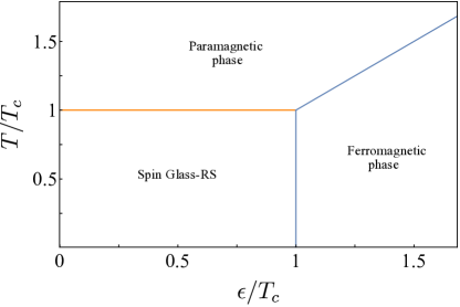
Figure 1: Phase diagram in the $(\epsilon,T)$ plane for the $p=2$ spherical spin glass, where $\epsilon$ represents the strength of two-body ferromagnetic interactions.

III Ordered non-linearity

The first perturbation to the spherical $p=2$ model that we have studied is represented by an ordered 4-body interaction term. The model is defined by the Hamiltonian

$$\mathcal{H}_{\text{ord}}(\boldsymbol{\sigma})=\mathcal{H}_{J}(\boldsymbol{\sigma})-\frac{4!\epsilon}{N^{3}}\sum_{i<j<k<l}^{1,N}\sigma_{i}\sigma_{j}\sigma_{k}\sigma_{l},$$ (9)

where $\mathcal{H}_{J}$ is the Hamiltonian (2) of the spherical $p=2$ model with $J_{0}=0$. The scaling of the ordered coupling magnitude is chosen in order for the non-linear term to be extensive. The parameter $\epsilon$ can be tuned to probe different regimes according to the strength of the non-linearity. The free energy of the model is obtained by means of a standard replica approach, which provides the exact mean-field solution in the large-$N$ limit.

For this model one has to consider two global order parameters

$$m_{a} =\frac{1}{N}\sum_{i=1}^{N}\sigma_{i}^{a}$$

$$q_{ab} =\frac{1}{N}\sum_{i=1}^{N}\sigma_{i}^{a}\sigma_{i}^{b},$$ (10)

where $m_{a}$ and $q_{ab}$ are respectively the magnetization elements and the overlap matrix elements. From here on, we will use the following symbols to denote the full overlap matrix and magnetization vector in replica space: $\mathbb{Q}=\{q_{ab}\}_{a,b=1,\ldots,n}$ and ${\bf m}=\{m_{a}\}_{a=1,\ldots,n}$. In terms of these order parameters the replicated partition function averaged over the disorder reads as

$$\overline{\mathcal{Z}^{n}} =\int\prod_{a<b}^{1,n}\text{d}q_{ab}\int\prod_{a=1}^{n}\text{d}m_{a}~{}e^{-NG[\mathbb{Q},{\bf m}]},$$ (11)

where the action functional $G$ is defined as

$$G[\mathbb{Q},{\bf m}]= -\frac{(\beta J)^{2}}{4}\sum_{ab}^{1,n}q_{ab}^{2}-\beta\epsilon\sum_{a=1}^{n}m_{a}^{4}$$ (12)

$$-\frac{1}{2}\ln\det(\mathbb{Q}-{\bf m}\otimes{\bf m}^{T}),$$ (13)

with

$$\beta\overline{f_{J}}=\lim_{n\rightarrow 0}\frac{1}{n}~{}\min_{m_{a}}~{}\max_{q_{ab}}~{}G[q_{ab},m_{a}].$$ (14)

In Eq. (12) the symbol ${\bf m}\otimes{\bf m}^{T}$ denotes a matrix with elements $({\bf m}\otimes{\bf m}^{T})_{ab}=m_{a}m_{b}$. Details on the derivation of $G[\mathbb{Q},{\bf m}]$ are given in App. A. As in standard replica approach, in order to find the physical value of the free energy we have to maximize with respect to the matricial order parameters and minimize with respect to the vectorial ones [11]. Stationary points are found by solving the following saddle-point equations:

$$\frac{\delta G}{\delta q_{ab}} =(\beta J)^{2}q_{ab}+(\mathbb{Q}-{\bf m}\otimes{\bf m}^{T})^{-1}_{ab}=0,$$ (15)

$$\frac{\delta G}{\delta m_{a}} =-4\beta\epsilon~{}m_{a}^{3}+[(\mathbb{Q}-{\bf m}\otimes{\bf m}^{T})^{-1}\cdot{\bf m}]_{a}=0.$$ (16)

In what follows we will present the results obtained within the RS ansatz for the matrix $q_{ab}$, which turns out to be stable for all values of temperature $T$ and strength $\epsilon$ of the non-linear coupling.

III.1 Replica Symmetric Ansatz

Let us then assume for the matrix $\mathbb{Q}$ a RS ansatz

$$q_{ab}=\delta_{ab}+(1-\delta_{ab})~{}q_{0}$$ (17)

For what concerns the vector ${\bf m}$ we must assume that all elements are identical, since physical quantities cannot depend on the replicas. By doing so we get

$$\left[(\mathbb{Q}-{\bf m}\otimes{\bf m}^{T})^{-1}\right]_{ab}=\left\{\begin{array}[]{rl}\cfrac{1-2q_{0}+m^{2}}{(1-q_{0})^{2}}~{}~{}~{}~{}a=b\\[12.0pt] -\cfrac{q_{0}-m^{2}}{(1-q_{0})^{2}}~{}~{}~{}~{}a\neq b.\end{array}\right.$$ (20)

The RS effective action reads, in the limit $n\rightarrow 0$, as

$$\lim_{n\rightarrow 0}\frac{1}{n}G[q_{0},m]= -\frac{(\beta J)^{2}}{4}(1-q_{0}^{2})-\beta\epsilon m^{4}$$ (21)

$$-\frac{1}{2}\ln(1-q_{0})-\frac{1}{2}\frac{q_{0}-m^{2}}{1-q_{0}}.$$

The RS saddle-point equations are obtained by plugging the ansatz (17) in Eqs. (15),(16) or by deriving Eq. (21) with respect to $q_{0}$ and $m$:

$$\frac{\partial G}{\partial q_{0}}= (\beta J)^{2}q_{0}-\frac{q_{0}-m^{2}}{(1-q_{0})^{2}}=0$$ (22)

$$\frac{\partial G}{\partial m}= -4\beta\epsilon m^{3}+\frac{m}{1-q_{0}}=0.$$ (23)

A trivial solution for Eq. (23) is $m=0$: in this case Eq. (22) simply becomes identical to the RS saddle-point equation for the original $p=2$ spherical model:

$$[1-(\beta J)^{2}(1-q_{0})^{2}]q_{0}=0.$$ (24)

The above equation has two solutions, corresponding to the two possible phases of the model: the paramagnetic phase with $q_{0}=0$, and the trivial spin-glass phase with $q_{0}=1-\frac{1}{\beta J}$. Eq. (23) admits also a $m\neq 0$ solution, which reads:

$$m^{2}=\frac{1}{4\beta\epsilon}\frac{1}{1-q_{0}},$$ (25)

that plugged into the equation for $q_{0}$ gives

$$q_{0}(1-q_{0})^{3}\left[\frac{1}{1-q_{0}}-(\beta J)^{2}\right]=\frac{1}{4\beta\epsilon}.$$ (26)

Summarizing, the analysis of the saddle-point equations obtained by assuming a RS ansatz yields overall three kind of solutions: the paramagnetic one with both $m=0$ and $q_{0}=0$; the solution corresponding to the trivial spin glass with $m=0$ and $q_{0}=1-1/(\beta J)$ and a ferromagnetic solution where both $m$ and $q_{0}$ are different from zero and are given by the solutions of Eqs. (25) and (26). The first two solutions are the only possible ones with $\epsilon=0$, that is the unperturbed case. The third solution is the interesting one in presence of non-linearity and can be studied numerically.

The following step of our analysis will consist in studying whether the ordered quartic non-linearity may trigger or not an instability of the RS ansatz, in particular whether or not it drives, in the low temperature regime, a transition from a trivial spin-glass phase to a true spin-glass phase with a non-trivial distribution of the overlap. In order to do that we need to study the stability of the RS solutions, which is the subject of the following section.

III.2 Stability of the RS solution and phase diagram

The nature of the fluctuations around the saddle point determines the stability of the solutions. By following [22], it is convenient to define a single array containing all variational parameters:

$$\boldsymbol{\eta}=\binom{{\bf m}}{[\mathbb{Q}]_{a\neq b}}.$$ (27)

The object defined in Eq. (27) is a vector in an $n(n+1)$-dimensional space, with element $\eta_{A}$ where the subscript index takes values in the range $A=1,\ldots,n(n+1)$. The number of variational parameters, with respect to which fluctuations must be taken into account, is $n(n+1)$ because we have to consider the $n$ components of ${\bf m}$ and $n(n-1)/2$ components for $\mathbb{Q}$, since for the overlap matrix the diagonal elements are fixed to $q_{aa}=1$ by the spherical constraint. The effective action (12) can be expanded around the saddle point $\boldsymbol{\eta}^{*}=(\boldsymbol{m}^{*},\mathbb{Q}^{*})$ up to the second order in the deviations from saddle-point solutions:

$$G[\boldsymbol{\eta}^{*}+\delta\boldsymbol{\eta}]=G[\boldsymbol{\eta}^{*}]+\frac{1}{2}\sum_{AB}\frac{\partial^{2}G[\boldsymbol{\eta}^{*}]}{\partial\eta_{A}\partial\eta_{B}}~{}\delta\eta_{A}\delta\eta_{B}+\ldots,$$

In Eq. (III.2) there are no linear terms because when $\boldsymbol{\eta}^{*}$ is selected as the solution of saddle-point equations we have by definition

$$\frac{\partial G[\boldsymbol{\eta}^{*}]}{\partial\eta_{A}}=0\quad\quad\quad\forall~{}A.$$ (29)

In order to assess the stability of the solution $\boldsymbol{\eta}^{*}$ one has to study the spectrum of the Hessian $\mathbb{H}_{AB}(\boldsymbol{\eta}^{*})=\partial^{2}G[\boldsymbol{\eta}^{*}]/\partial\eta_{A}\partial\eta_{B}$. By explicitating the dependence on the overlap and magnetization fluctuations, the expansion in Eq. (III.2) can be rewritten as:

$$G[\mathbb{Q},{\bf m}]=G[\mathbb{Q}^{*},{\bf m}^{*}]+\frac{1}{2}\sum_{ab}\frac{\partial^{2}G[\mathbb{Q}^{*},{\bf m}^{*}]}{\partial m_{a}\partial m_{b}}\delta m_{a}\delta m_{b}+\sum_{ab,c}\frac{\partial^{2}G[\mathbb{Q}^{*},{\bf m}^{*}]}{q_{ab}\partial m_{c}}\delta q_{ab}\delta m_{c}+\frac{1}{2}\sum_{ab,cd}\frac{\partial^{2}G[\mathbb{Q}^{*},{\bf m}^{*}]}{\partial q_{ab}\partial q_{cd}}\delta q_{ab}\delta q_{cd}+...$$ (30)

It is well known that, in the limit $n\rightarrow 0$, the smallest eigenvalue of the Hessian $\mathbb{H}[\boldsymbol{\eta}^{*}]$ is the replicon [22], which is related only to overlap fluctuations and can be obtained from the diagonalization of the submatrix

$$G_{(ab),(cd)}=\frac{\partial^{2}G[\mathbb{Q}^{*},{\bf m}^{*}]}{\partial q_{ab}\partial q_{cd}}.$$ (31)

In general, i.e. without specifying the solution ansatz for the saddle point, this matrix has three different kinds of elements, defined by taking: (i) $a=c$ and $b=d$; (ii) either $a\neq c$ and $b=d$ or $a=c$ and $b\neq d$; (iii) $a\neq c$ and $b\neq d$. These elements are related to different correlations of the replicated local variables, as can be immediately recognized in the case of a model with Ising variables (see Ref. [22] for the RS case). In the case of spherical variables, we can rewrite the action functional (12) in the following way

$$G[\mathbb{Q} ,{\bf m}]=-\frac{(\beta J)^{2}}{2}\sum_{a<b}^{1,n}q_{ab}^{2}-\beta\epsilon\sum_{a=1}^{n}m_{a}^{4}$$ (32)

$$+\ln\int\prod_{a=1}^{n}\text{d}x_{a}e^{-\sum_{a\leq b}^{n}[(\mathbb{Q}-{\bf m}\otimes{\bf m}^{T})^{-1}]_{ab}x_{a}x_{b}},$$

where we have introduced back the local variables as correlated Gaussian auxiliary variables to represent the entropic term  $\ln\det(\mathbb{Q}-{\bf m}\otimes{\bf m}^{T})$. With this formalism, we have

$$\frac{\partial G[\mathbb{Q},{\bf m}]}{\partial q_{ab}}=-(\beta J)^{2}q_{ab}-\langle x_{a}x_{b}\rangle,$$ (33)

where the average is computed over the Gaussian distribution of the $x_{a}$ variables:

$$\langle\cdots\rangle=\frac{\int\prod_{a=1}^{n}\text{d}x_{a}e^{-\sum_{a\leq b}^{n}(\mathbb{Q}-{\bf m}\otimes{\bf m}^{T})_{ab}x_{a}x_{b}}(\cdots)}{\int\prod_{a=1}^{n}\text{d}x_{a}e^{-\sum_{a\leq b}^{n}(\mathbb{Q}-{\bf m}\otimes{\bf m}^{T})_{ab}x_{a}x_{b}}}.$$ (34)

Therefore, by using the fact that

$$\frac{\partial}{\partial q_{cd}}\langle x_{a}x_{b}\rangle=-\langle x_{a}x_{b}x_{c}x_{d}\rangle+\langle x_{a}x_{b}\rangle\langle x_{c}x_{d}\rangle,$$ (35)

we have

$$G_{(ab),(ab)}\equiv\frac{\partial^{2}G}{\partial q_{ab}^{2}}=-(\beta J)^{2}+\langle x_{a}^{2}x_{b}^{2}\rangle-\langle x_{a}x_{b}\rangle^{2}$$ (36a)

$$G_{(ab),(ac)}\equiv\frac{\partial^{2}G}{\partial q_{ac}\partial q_{ab}}=\langle x_{a}^{2}x_{b}x_{c}\rangle-\langle x_{a}x_{b}\rangle\langle x_{a}x_{c}\rangle$$ (36b)

$$G_{(ab),(cd)}\equiv\frac{\partial^{2}G}{\partial q_{cd}\partial q_{ab}}=\langle x_{a}x_{b}x_{c}x_{d}\rangle-\langle x_{a}x_{b}\rangle\langle x_{c}x_{d}\rangle.$$ (36c)

We can now use Wick’s theorem to compute the contractions of the 4-point Gaussian correlators and express them in terms of the second moment of the Gaussian distribution. We have

$$G_{(ab),(ab)}=-(\beta J)^{2}+\langle x_{a}^{2}\rangle\langle x_{b}^{2}\rangle+\langle x_{a}x_{b}\rangle^{2}$$ (37a)

$$G_{(ab),(ac)}=\langle x_{a}^{2}\rangle\langle x_{b}x_{c}\rangle+\langle x_{a}x_{b}\rangle\langle x_{a}x_{c}\rangle$$ (37b)

$$G_{(ab),(cd)}=\langle x_{a}x_{c}\rangle\langle x_{b}x_{d}\rangle+\langle x_{a}x_{d}\rangle\langle x_{b}x_{c}\rangle,$$ (37c)

where

$$\langle x_{a}x_{b}\rangle=\left[(\mathbb{Q}-{\bf m}\otimes{\bf m}^{T})^{-1}\right]_{ab}.$$ (38)

III.2.1 Replicon

The diagonalization of $G_{(ab),(cd)}$ has to be performed case by case depending on the solution ansatz for the saddle point problem. If $(\mathbb{Q}^{*},{\bf m}^{*})$ is a RS saddle point, due to the symmetry of the overlap matrix $\mathbb{Q}^{*}$ under the permutation of $n$ replicas, $G_{(ab),(cd)}$ depends only on three numbers:

$$P=-(\beta J)^{2}+\langle x_{a}^{2}\rangle^{2}+\langle x_{a}x_{b}\rangle^{2}$$ (39a)

$$Q=\langle x_{a}^{2}\rangle\langle x_{a}x_{b}\rangle+\langle x_{a}x_{b}\rangle^{2}$$ (39b)

$$R=2\langle x_{a}x_{b}\rangle^{2}.$$ (39c)

Therefore, the eigenvalues of $G_{(ab),(cd)}$ depend on combinations of $P,Q$ and $R$ and can be computed in a straightforward manner by following the procedure of Ref. [22] or by using the Replica Fourier Transform [14, 23]. There are three types of eigenvalues at finite $n$: the longitudinal one, corresponding to fluctuations of the overlap which do not break the replica symmetry, the anomalous one, corresponding to fluctuations which break the replica symmetry, but violate the property of the overlap matrix of having the same sum over each row, and the replicon, connected to fluctuations which break the replica symmetry preserving the properties of the overlap matrix. In the limit $n\rightarrow 0$, the longitudinal and anomalous eigenvalues degenerate in the same one. The replicon has the following expression:

$$\begin{split}\lambda_{R}&=P-2Q+R\\ &=-(\beta J)^{2}+\left(\langle x_{a}^{2}\rangle-\langle x_{a}x_{b}\rangle\right)^{2}.\end{split}$$ (40)

The expression in Eq. (20) for $(\mathbb{Q}-{\bf m}\otimes{\bf m}^{T})^{-1}$ in the RS case implies that the explicit expression of the replicon is

$$\lambda_{R}=-(\beta J)^{2}+\frac{1}{(1-q_{0})^{2}}.$$ (41)

For RSB saddle points, the diagonalization of the Hessian matrix is more difficult, since the three different kinds of elements in Eq. (36) have more than just three possible values. The computation for the fluctuations around a 1RSB saddle point can be found in Ref. [24], while the generalization to generic $k$-RSB saddle points can be found in Ref. [25]. But for the present case this further step of the calculation is not necessary, since the RS ansatz turns out to be always stable.

III.2.2 Phase diagram

The phase diagram of the model with ordered $p=4$ interaction, represented by the Hamiltonian in Eq. (9), is then obtained by looking for the solutions of the RS saddle-point equations, Eqns. (22)(23), and studying their stability. The result of this analysis is presented in Fig. 2. For $T>T_{c}$ and small values of $\epsilon$ the system is in a paramagnetic phase, which is stable because the replicon is always positive, as can be checked by plugging into Eq. (41) the values $q_{0}=0$ and $T>T_{c}=J$.

Then, for small values of $\epsilon$ by lowering the temperature below $T_{c}$ the system passes to a trivial spin-glass phase, which is marginally stable, since $\lambda_{R}=0$ in all this region of the parameters as can be checked by using the expression $q_{0}=1-\frac{1}{\beta J}$ in Eq. (41). On the contrary, if $\epsilon$ is large enough and the non-linear ferromagnetic interaction prevails on the disordered two-body interaction, that is for $\epsilon\gtrsim 1.5$, upon lowering the temperature there is no spin-glass transition and the system moves directly to the ferromagnetic phase. By using Eqs. (26) and (41) one finds the expression

$$\lambda_{R}=\frac{1}{4\beta\epsilon q_{0}(1-q_{0})^{3}}$$ (42)

from which one concludes that $\lambda_{R}>0$ for all values of $q_{0}\in[0,1]$. We also find a small interval of $\epsilon$ values, approximately $\epsilon\in[0.85:1.5]$ where at $T=T_{c}$ the system encounters first a transition to the (trivial) spin-glass phase and then, upon lowering further the temperature, a transition from (trivial) spin-glass to the ferromagnetic phase. Let us stress that in the phase diagram of Fig. 2 the transition line which separates the ferromagnetic phase from the other phases is a line of first order transitions: the paramagnetic phase and the trivial spin glass phase, respectively at temperatures above and below the critical one, are always stable upon increasing $\epsilon$ and the transition to the ferromagnetic phase is controlled by the free-energy balance.

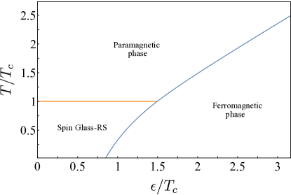
Figure 2: Phase diagram in the $(\epsilon,T)$ plane for the $p=2$ spherical spin glass plus four-body ferromagnetic interactions, where $\epsilon$ represents the strength of 4-body ferromagnetic interactions.

We can therefore conclude that the addition of ordered non-linear interactions does not produce any sort of RSB in the trivial spin glass phase of the spherical model. By comparing the present result with the phase diagram in Fig. 1 we can remark a behaviour which is topologically analogous, upon increasing the strength of the non-linearity $\epsilon$, to that of the $p=2$ spherical model with ferromagnetic two-body interactions competing with the disordered ones [13]: the trivial spin-glass phase remains marginally stable until the point where a transition to ferromagnetic order takes place.

Notice also, that this scenario holds for arbitrary ordered non-linearity, as one can see with a straightforward generalization of the previous analysis. If we denote by $p$ the power of the non-linearity, the only change in the action (12) is that the magnetization term is raised to the power $p$. As a consequence the RS saddle point equation obtained deriving the action w.r.t $q_{0}$ (22) remains the same and that obtained deriving w.r.t. $m$ reads

$$p\beta\epsilon m^{p-1}+\frac{m}{1-q_{0}}=0.$$ (43)

Therefore, the only change is in the equation for the overlap in the ferromagnetic phase, which reads

$$q_{0}(1-q_{0})^{\frac{2(p-1)}{p-2}}\left[\frac{1}{1-q_{0}}-(\beta J)^{2}\right]=\frac{1}{(p\beta\epsilon)^{\frac{2}{p-2}}},$$ (44)

from which one immediately recognize that

$$\lambda_{R}=\left(\frac{1}{p\beta\epsilon q_{0}(1-q_{0})^{p-1}}\right)^{\frac{2}{p-2}}>0$$ (45)

for all values of $p,\beta,\epsilon$ and $q_{0}\in[0,1]$.

IV Purely disordered nonlinearity

In this section we consider a different kind of perturbation to the spherical $p=2$ model, namely we added a 4-body interaction term with quenched random couplings. The model is defined by the Hamiltonian

$$\mathcal{H}_{\text{dis}}(\boldsymbol{\sigma})=\mathcal{H}_{J}(\boldsymbol{\sigma})-\sum_{i<j<k<l}^{1,N}J^{(4)}_{ijkl}~{}\sigma_{i}\sigma_{j}\sigma_{k}\sigma_{l},$$ (46)

where the couplings $J_{ijkl}$ are i.i.d. random variables following the Gaussian distribution

$$p(J_{ijkl})=\frac{1}{\sqrt{2\pi\sigma_{4}^{2}}}e^{-\frac{J_{ijkl}^{2}}{2\sigma_{4}^{2}}},$$ (47)

with variance

$$\sigma_{4}^{2}=\frac{\epsilon^{2}~{}4!}{2N^{3}}.$$ (48)

By averaging over the disorder, one reaches the following form for the replicated partition function:

$$\overline{\mathcal{Z}^{n}} =\int\prod_{a<b}^{1,n}\text{d}q_{ab}~{}e^{-NG[\mathbb{Q}]},$$ (49)

where the action $G[\mathbb{Q}]$ is defined as

$$G[\mathbb{Q}]= -\frac{(\beta J_{2})^{2}}{2}\sum_{a\leq b}^{1,n}q_{ab}^{2}-\frac{(\beta\epsilon)^{2}}{2}\sum_{a\leq b}^{1,n}q_{ab}^{4}$$ (50)

$$-\frac{1}{2}\ln\det\mathbb{Q}.$$

The one above is the free energy of the so-called mixed $p$-spin model, whose equilibrium thermodynamics has been studied extensively in [15, 16], while more recent and very interesting results on the dynamics can be found in [26, 27]. Let us notice that in the present case, at variance with the model studied in Sec. III, due to the absence of any ferromagnetic term in the Hamiltonian there is only one ordered parameter, the overlap matrix $\mathbb{Q}$.

IV.1 RS saddle-point equations and stability

The RS free energy of the $2+4$-spin model, obtained through steps analogous to those reported in App. A, reads as

$$\lim_{n\rightarrow 0}\frac{1}{n}G[q_{0}]= -\frac{(\beta J_{2})^{2}}{4}(1-q_{0}^{2})-\frac{(\beta\epsilon)^{2}}{4}(1-q_{0}^{4})$$ (51)

$$-\frac{1}{2}\ln(1-q_{0})-\frac{1}{2}\frac{q_{0}}{1-q_{0}},$$

from which the saddle point equation in $q_{0}$ is

$$q_{0}\left[(\beta J_{2})^{2}+2(\beta\epsilon)^{2}q_{0}^{2}-\frac{1}{(1-q_{0}^{2})}\right]=0.$$ (52)

By proceeding in a similar way with respect to Sec. III.2, we rewrite the effective action as

$$G[\mathbb{Q}]= -\frac{(\beta J_{2})^{2}}{2}\sum_{a<b}^{1,n}q_{ab}^{2}-\frac{(\beta\epsilon)^{2}}{2}\sum_{a<b}^{1,n}q_{ab}^{4}$$ (53)

$$+\ln\int\prod_{a=1}^{n}\text{d}x_{a}e^{-\sum_{a\leq b}^{n}q_{ab}x_{a}x_{b}},$$

from which the expressions for the stability matrix elements read as

$$G_{(ab),(ab)}=-(\beta J_{2})^{2}-6(\beta\epsilon)^{2}q_{ab}^{2}+\langle x_{a}^{2}\rangle\langle x_{b}^{2}\rangle+\langle x_{a}x_{b}\rangle^{2}$$ (54a)

$$G_{(ab),(ac)}=\langle x_{a}^{2}\rangle\langle x_{b}x_{c}\rangle+\langle x_{a}x_{b}\rangle\langle x_{a}x_{c}\rangle$$ (54b)

$$G_{(ab),(cd)}=\langle x_{a}x_{c}\rangle\langle x_{b}x_{d}\rangle+\langle x_{a}x_{d}\rangle\langle x_{b}x_{c}\rangle,$$ (54c)

where in this case

$$\langle x_{a}x_{b}\rangle=(q^{-1})_{ab}.$$ (55)

By recalling the general expression for the replicon in the case of RS ansatz, given in Eq. (40), we obtain in the present case

$$\lambda_{R}=-(\beta J_{2})^{2}-6(\beta\epsilon)^{2}q_{0}^{2}+\frac{1}{(1-q_{0})^{2}}.$$ (56)

By plugging the expression of Eq. (52) into Eq. (56) it is easy to realize that $\lambda_{R}$ is negative for any value of the parameter $q_{0}$ different from zero, so that in the RS case only the solution $q_{0}=0$ can be stable. By then plugging the latter into the expression of the replicon we get $\lambda_{R}=1-(\beta J_{2})^{2}$, which for temperatures $T<T_{c}=J_{2}$ becomes negative, signalling the instability of the RS ansatz and therefore forcing us to consider RSB solutions.

IV.2 1RSB saddle-point equations

The first attempt to go beyond a RS ansatz it is always represented by considering one step of replica symmetry breaking (1RSB), corresponding to an overlap matrix, which we may refer to as $\mathbb{Q}^{\text{1step}}$, with the following structure:

$$[\mathbb{Q}^{\text{1step}}]_{ab}=(1-q_{1})\delta_{ab}+(q_{1}-q_{0})\epsilon_{ab}+q_{0}\mathbb{I}_{ab}.$$ (57)

$\mathbb{I}={\bf 1}\otimes{\bf 1}^{T}$ is a matrix whose elements are all identically equal to $1$, while $\epsilon$ is a block diagonal matrix, with diagonal blocks all equal to $\mathbb{I}_{x}={\bf 1}_{x}\otimes{\bf 1}_{x}^{T}$, namely $x\times x$ square matrices with all elements identically equal to one. For the 1RSB ansatz we have therefore three variational parameters: $q_{0}$, $q_{1}$ and $x$. In the present case the inverse matrix of matrix $q_{ab}$ reads as:

$$[(\mathbb{Q}^{\text{1step}})^{-1}]_{ab}=A\delta_{ab}+B\epsilon_{ab}+C\mathbb{I}_{ab},$$ (58)

with

$$A=\frac{1}{1-q_{1}}$$ (59)

$$B=-\frac{(q_{1}-q_{0})}{(1-q_{1})(1-q_{1}+x(q_{1}-q_{0}))}$$ (60)

$$C=-\frac{q_{0}}{[1-q_{1}+x(q_{1}-q_{0})]^{2}}.$$ (61)

Given this structure of the overlap matrix, with very similar calculations to the RS case and defining the function

$$\chi_{p}=\chi_{p}(q_{0},q_{1},x)\equiv 1-q_{1}^{p}+x(q_{1}^{p}-q_{0}^{p}),$$ (62)

we get as 1RSB effective action:

$$\lim_{n\rightarrow 0}\frac{1}{n}G[q_{0},q_{1},x]=-\frac{(\beta J_{2})^{2}}{4}\chi_{2}-\frac{(\beta\epsilon)^{2}}{4}\chi_{4}-$$

$$\frac{x-1}{2x}\log(1-q_{1})-\frac{1}{2x}\log(\chi_{1})-\frac{1}{2}\frac{q_{0}}{\chi_{1}}.$$

The 1RSB saddle point equations read as:

$$\frac{\partial G}{\partial q_{0}}=\frac{x}{2}q_{0}\left[(\beta J_{2})^{2}+2(\beta)^{2}q_{0}^{2}-\frac{1}{\chi_{1}^{2}}\right]=0,$$ (63a)

$$\frac{\partial G}{\partial q_{1}}=(x-1)\left[-q_{1}(\beta J_{2})^{2}-2q_{1}^{3}(\beta\epsilon)^{2}+\frac{q_{0}}{\chi_{1}^{2}}+\frac{q_{1}-q_{0}}{(1-q_{1})\chi_{1}}\right]=0,$$ (63b)

$$\frac{\partial G}{\partial x}=-\frac{(\beta J_{2})^{2}}{2}[q_{1}^{2}-q_{0}^{2}]-\frac{(\beta\epsilon)^{2}}{2}[q_{1}^{4}-q_{0}^{4}]+\frac{1}{x^{2}}\log\frac{\chi_{1}}{1-q_{1}}+(q_{1}-q_{0})\left[\frac{q_{0}}{\chi_{1}^{2}}-\frac{1}{x\cdot\chi_{1}}\right]=0.$$ (63c)

IV.3 Stability of the 1RSB saddle point and phase diagram

For the diagonalization of the stability matrix of the 1RSB ansatz we have followed the procedure of [24], which generalizes RS calculations of [22].

IV.3.1 Replicon

There are three different classes of fluctuations around the 1RSB saddle point, leading to nine different eigenvalues, which reduce to seven in the limit $n\rightarrow 0$. Following [15, 16], the two relevant eigenvalues for the study of the stability are

$$\Lambda^{(1)}=-(\beta J_{2})^{2}-6(\beta\epsilon)^{2}q_{1}^{2}+\frac{1}{(1-q_{1})^{2}}$$ (64)

$$\Lambda^{(2)}=-(\beta J_{2})^{2}-6(\beta\epsilon)^{2}q_{0}^{2}+\frac{1}{(1-q_{1}+x(q_{1}-q_{0}))^{2}}.$$ (65)

Fluctuations with respect to a given ansatz for the breaking of replica symmetry means fluctuations which alter the structure of the matrix $\mathbb{Q}^{\text{1step}}$. In general for these instabilities it is also possible to give a physical interpretation connected to the modification of the matrix structure. In particular, in the case of a block diagonal matrix $\mathbb{Q}^{\text{1step}}$, each row of the matrix has the same structure: one element is unity, there are $x-1$ elements equal to $q_{1}$, those belonging to the same block $\mathbb{I}_{x}$, and $n-x$ elements equal to $q_{0}$. This structure of the matrix corresponds to a “one-step” fragmentation of phase space in disjoint ergodic components, which we may refer to as states or clusters. Configurations belonging to the same state have typical overlap $q_{1}$, while configurations belonging to different states have overlap $q_{0}$. By considering the structure of the matrix $\mathbb{Q}^{\text{1step}}$, a consistent interpretation is to regard the elements of blocks $\mathbb{I}_{x}$ as the typical overlap between configurations belonging to the same state and the elements outside blocks $\mathbb{I}_{x}$ as the typical overlap between configurations belonging to different states.

Given this scenario, we consider two kind of instabilities: 1) a single state can undergo a further fragmentation process, which corresponds to an emerging block structure inside $\mathbb{I}_{x}$, with new elements $q_{2}$ appearing within $\mathbb{I}_{x}$ (again in a block-diagonal structure); 2) different states can merge into a single one, which corresponds to a rearrangement of the structure of the whole $\mathbb{Q}^{\text{1step}}$, with all inner elements of different blocks $\mathbb{I}_{x}$ changing value from $q_{1}$ to $q_{2}$ and some of the extra-block elements rising from $q_{0}$ to $q_{1}$. These two patterns to alter the 1RSB structure of $\mathbb{Q}^{\text{1step}}$ are connected respectively to the eigenvalues $\Lambda^{(1)}$ and $\Lambda^{(2)}$. In particular, the fluctuations inside the same cluster represented by $\Lambda^{(1)}$ are the ones which destabilize the 1RSB phase in the SK model and that lead, across an infinite sequences of further other breakings, to the well known fractal free-energy structure [10]. This instability pattern for the 1RSB phase is the most common: it is for instance the one which is also found in models of hard spheres [5, 7] and ecological models [4].

On the other hand, for mixed $p$-spin models, i.e., models with spherical variables and competition between linear and non-linear interactions, it turns out the dominant instabilities are those related to $\Lambda^{(2)}$, as demonstrated in [16] by showing that $\Lambda^{(1)}>\Lambda^{(2)}$, so that the latter is the dominant eigenvalue. This means that the relevant replicon is the one related to fluctuations between clusters. In this situation it was pointed out in [16] that an intermediate phase also emerges, the so-called 1-full-RSB phase, characterized by the coexistence between a one-step and full replica symmetry breaking (full-RSB). In the present discussion we will not deem to study in detail the transition between this mixed 1-full-RSB phase and the pure full-RSB phase, which also takes place in the present case, referring the interested reader to [16].

IV.3.2 Phase diagram

In the mixed $p$-spin with purely disordered nonlinearity we keep fixed the variance of the two-body disordered interaction, as in the previous study of Sec. III, and study the phase diagram in the plane $(\epsilon,T)$, where in the present case $\epsilon$ represents the standard deviation of the four-body couplings disorder. As in the previous case, we find that the lower limit of stability of the paramagnetic phase is $T_{c}=J_{2}$. For $\epsilon$ high enough one finds at all temperatures a transition to a 1RSB glassy phase. Then, depending on the temperature, upon lowering $\epsilon$ we can either find a transition to the paramagnetic phase, for $T>T_{c}$, or a transition to a full-RSB phase, for $T<T_{c}$, (either 1-full-RSB or standard full-RSB).

Let us remark the difference between the transition taking place from the 1-RSB phase to the paramagnetic one above $T_{c}$ and the one taking place from the 1-RSB to the full-RSB below $T_{c}$. Considering the probability distribution of the overlap between replicas, which corresponds to the parametrization of the matrix $\mathbb{Q}^{\text{1step}}$, the transition at temperatures $T>T_{c}$ has the features of a first-order phase transition, and is in fact usually known as “Random First-Order Transition” [28, 29], while the transition at temperatures $T<T_{c}$ has the features of a second order phase transition. This means that for $T>T_{c}$, upon reducing $\epsilon$, the 1RSB ansatz for $\mathbb{Q}^{\text{1step}}$ is always a locally stable solution, even when it becomes less convenient than the RS ansatz from the point of view of free energy, until when it completely disappears as a solution at the line marked in the phase diagram as 1RSB spinodal. This is the transition mechanism typical of first-order transitions. Technically, the spinodal line is simply obtained looking for the value of $\epsilon$ where non-trivial solutions of the equation $\partial G/\partial q_{1}=0$ arise in terms of $q_{1}$ with $x=1$ and $q_{0}=0$ fixed, for instance by increasing $\epsilon$ at fixed temperature $T$.

On the other hand, for $T<T_{c}$, the transition from the 1RSB phase to the full-RSB phase takes place when the former loses stability in favour of the latter, as happens typically in second order phase transitions. The transition line in Fig. 3 has been obtained by finding the values of the parameters where $\Lambda^{(2)}=0$. Despite this difference concerning the behaviour of the overlap matrix, both transitions are continuous from the point of view of Landau classification, because in both cases there is no latent heat.

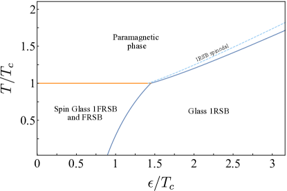
Figure 3: Phase diagram in the $(\epsilon,T)$ plane for the $p=2$ spherical spin glass plus four-body purely disordered interactions, where $\epsilon$ represents the strength of non-linear interactions.

V Ferromagnetic+disordered non-linearity

Having assessed the effect of adding respectively purely ordered and purely disordered non-linear terms to the $p=2$ spherical model, in this section we study the effect of non-linear terms with both competing disordered and ferromagnetic interactions. This can be done by extracting the couplings of the 4-body interaction term from a non-zero average probability distribution, namely we consider

$$p(J_{ijkl})=\frac{1}{\sqrt{2\pi\sigma_{4}^{2}}}e^{-\frac{(J_{ijkl}-J_{0})^{2}}{2\sigma_{4}^{2}}},$$ (66)

with

$$\sigma_{4}^{2}=\frac{\epsilon^{2}~{}4!}{2N^{3}}~{}~{}~{}~{}~{}~{}~{}J_{0}=\frac{\epsilon^{2}~{}4!}{N^{3}}.$$ (67)

The variable $\epsilon$ parametrizes both the mean and the variance of the 4-body couplings distribution. This choice allows to have just one free parameter for the whole Gaussian distribution. With a similar computation with respect to the previous cases we find the effective action

$$\begin{split}G[\mathbb{Q},{\bf m}]=&-\frac{(\beta J)^{2}}{2}\sum_{a<b}^{1,n}q_{ab}^{2}-\frac{(\beta\epsilon)^{2}}{2}\sum_{a<b}^{1,n}q_{ab}^{4}\\ &-\beta\epsilon^{2}\sum_{a=1}^{n}m_{a}^{4}-\frac{1}{2}\ln\det\left(\mathbb{Q}-{\bf m}\otimes{\bf m}^{T}\right).\end{split}$$ (68)

V.1 RS solutions

In the same way of previous sections we begin by considering a RS ansatz for the matrix $\mathbb{Q}$. This leads to a RS action reading as:

$$\lim_{n\rightarrow 0}\frac{1}{n}G[q_{0}, m]=-\frac{(\beta J_{2})^{2}}{4}(1-q_{0}^{2})-\frac{(\beta\epsilon)^{2}}{4}(1-q_{0}^{4})$$

$$-\beta\epsilon^{2}m^{4}-\frac{1}{2}\log(1-q_{0})-\frac{1}{2}\frac{q_{0}-m^{2}}{1-q_{0}}.$$ (69)

The RS saddle-point equations read as:

$$\frac{\partial G}{\partial q_{0}} =(\beta J_{2})^{2}q_{0}+2\beta^{2}\epsilon^{2}q_{0}^{3}-\frac{q_{0}-m^{2}}{(1-q_{0})^{2}}=0$$

$$\frac{\partial G}{\partial m} =-4\beta\epsilon^{2}m^{3}+\frac{m}{1-q_{0}}=0$$ (70)

There are three possible solutions for Eq. (70):

1. $m=0$;
   $q_{0}=0$.

2. $m=0$;
   $(\beta J_{2})^{2}+2\beta^{2}\epsilon^{2}q_{0}^{2}=1/(1-q_{0})^{2}$.

3. $m=1/\sqrt{4\beta\epsilon^{2}(1-q_{0})}$;
   $q_{0}(1-q_{0})[1-(1-q_{0})^{2}((\beta J_{2})^{2}+2\beta^{2}\epsilon^{2}q_{0}^{2})]=1/(4\beta\epsilon^{2})$.

In order to study the stability of the solution we have computed the replicon, which for the present case reads as:

$$\lambda_{R}=\frac{1}{(1-q_{0})^{2}}-(\beta J_{2})^{2}-6\beta^{2}\epsilon^{2}q_{0}^{2}.$$ (71)

The paramagnetic solution (PM, n.1) with $m=0$ and $q_{0}=0$ is unstable everywhere below the critical line $T_{c}=J_{2}$, since $\lambda_{R}>0$. Therefore, below this line, which is the horizontal orange one in the phase diagram of Fig. 4, we can only have phases with either finite magnetization or replica symmetry breaking or both. The trivial spin glass solution (n.2), is never stable for this model because one always has $\lambda_{R}<0$, therefore it is always excluded from the phase diagram. For what concerns the ferromagnetic phase (FM, n.3) in the list above, the numerical solution of the corresponding saddle-point equations shows that in the range of parameters $(\epsilon,T)$ where such a solution exists and is nontrivial, it is stable, i.e. $\lambda_{R}>0$.

Regarding the PM-FM transition, since both solutions are always stable, it is only by comparing their free energies that we can determine the transition line. The coordinates of this first-order transition line in the phase diagram in Fig. 4 are obtained by the implicit equation:

$$f^{\text{para}}(\epsilon_{c}^{\text{ferro}},T_{c}^{\text{ferro}})=f^{\text{ferro}}(\epsilon_{c}^{\text{ferro}},T_{c}^{\text{ferro}}),$$ (72)

where:

$$\text{sol n.1}~{}~{}\Longrightarrow~{}~{} f^{\text{para}}(\epsilon,T)=\frac{1}{\beta}G(q_{0}=0,m=0)$$

$$=-\frac{\beta}{4}(J_{2}^{2}+\epsilon^{2})$$

$$\text{sol n.3}~{}~{}\Longrightarrow~{}~{} f^{\text{ferro}}=G(q_{0}>0,m>0).$$ (73)

We will comment the remaining part of the phase diagram, namely what happens at temperatures lower than the critical one for the stability of the paramagnetic phase, $T<T_{c}$, in the following paragraph after having introduced the 1RSB ansatz for the replica matrix.

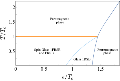
Figure 4: Phase diagram in the $(\epsilon,T)$ plane for the $p=2$ spherical spin glass plus four-body interactions, with competing disordered and ferromagnetic terms, where the variance of the disorder and the strength of ferromagnetic couplings are both controlled by $\epsilon$, see Eq. (67) in the text.

V.2 1RSB ansatz

In order to study the phase diagram of the model for $T<T_{c}$ we need to consider the possibility of replica symmetry breaking. By recalling the definition

$$\chi_{p}(q_{0},q_{1},x) =1-q_{1}^{p}+x(q_{1}^{p}-q_{0}^{p})$$ (74)

and by assuming the 1RSB structure for the matrix $\mathbb{Q}$ we obtain the following form for the effective action in the limit $n\rightarrow 0$:

$$\lim_{n\rightarrow 0}\frac{1}{n}G[q_{0},q_{1},x,m]=-\frac{(\beta J_{2}^{2})^{2}}{4}\chi_{2}(q_{0},q_{1},x)-\frac{\beta^{2}\epsilon^{2}}{4}\chi_{4}(q_{0},q_{1},x)-\beta\epsilon^{2}m^{4}-\frac{x-1}{2x}\ln(1-q_{1})-\frac{\ln(\chi_{1})}{2x}-\frac{q_{0}-m^{2}}{2\chi_{1}(q_{0},q_{1},x)},$$

from which the four 1RSB saddle point equations read as:

$$\frac{\partial G}{\partial q_{0}} =\frac{(\beta J_{2})^{2}}{2}xq_{0}+\beta^{2}\epsilon^{2}xq_{0}^{3}-\frac{1}{2}\frac{(q_{0}-m^{2})x}{\chi_{1}^{2}(q_{0},q_{1},x)}=0$$

$$\frac{\partial G}{\partial q_{1}} =(x-1)\bigg{[}-\frac{(\beta J_{2})^{2}}{2}q_{1}-\beta^{2}\epsilon^{2}q_{1}^{3}+\frac{1}{2x(1-q_{1})}-\frac{1}{2x\chi_{1}(q_{0},q_{1},x)}+\frac{q_{0}-m^{2}}{2\chi_{1}^{2}(q_{0},q_{1},x)}\bigg{]}=0$$

$$\frac{\partial G}{\partial x} =-\frac{(\beta J_{2})^{2}}{4}(q_{1}^{2}-q_{0}^{2})-\frac{\beta^{2}\epsilon^{2}}{4}(q_{1}^{4}-q_{0}^{4})-\frac{1}{2}\frac{q_{1}-q_{0}}{x\chi_{1}(q_{0},q_{1},x)}+\frac{1}{2x^{2}}\ln\left(1+\frac{x(q_{1}-q_{0})}{1-q_{1}}\right)+\frac{(q_{0}-m^{2})(q_{1}-q_{0})}{2\chi_{1}^{2}(q_{0},q_{1},x)}=0$$

$$\frac{\partial G}{\partial m} =m\left(-4\beta\epsilon^{2}m^{2}+\frac{1}{\chi_{1}(q_{0},q_{1},x)}\right)=0.$$ (76)

The expression of the two replicon eigenvalues which are relevant in the limit $n\rightarrow 0$, which can be obtained following the lines of [16], reads as

$$\Lambda^{(1)}[q_{1}]=-(\beta J_{2})^{2}-6\beta^{2}\epsilon^{2}q_{1}^{2}+\frac{1}{(1-q_{1})^{2}},$$ (77)

$$\Lambda^{(2)}[q_{0},q_{1},x]=-(\beta J_{2})^{2}-6\beta^{2}\epsilon^{2}q_{0}^{2}+\frac{1}{(1-q_{1}+x(q_{1}-q_{0}))^{2}}.$$ (78)

As already mentioned, for this model the most relevant between the two is $\Lambda^{(2)}$, signalling a pattern of instability of the 1RSB ansatz characterized by the merging of 1RSB clusters.

V.2.1 Phase Diagram

Let us here summarize how all the transition lines for $T<T_{c}$ in Fig. 4 have been obtained. We find, for $\epsilon$ large enough, a stable 1RSB phase with zero magnetization, $m=0$. The transition line which separates this 1RSB phase, which we refer to simply as glass phase, from the spin-glass phase (with full-RSB) at smaller value of $\epsilon$ has been determined by simply tracking the value of the control parameters where the 1RSB phase loses stability. That is, the intrinsic equation of this line is determined as

$$\Lambda^{(2)}[q_{0}(\epsilon_{c}^{sg},T_{c}^{sg}),q_{1}(\epsilon_{c}^{sg},T_{c}^{sg}),x(\epsilon_{c}^{sg},T_{c}^{sg})]=0.$$ (79)

Inside the region of the phase diagram delimited by the lines $T=T_{c}$ above and $(\epsilon_{c}^{sg},T_{c}^{sg})$ to the right, both the RS and the 1RSB solutions are unstable. This is therefore necessarily a region where further breakings of the symmetry between replica occurs. As already mentioned, we know from the results of [15] that different kinds of full-RSB occur here. Both the transitions occourring along these lines are continuous.

Finally, the transition line at $T<T_{c}$ between the RS ferromagnetic phase at large $\epsilon$ and the intermediate zero magnetization 1RSB phase at smaller values of $\epsilon$ is determined by simply comparing their free energies and has the implicit equation:

$$f^{\text{ferro}}(\epsilon_{c}^{\text{ferro/1rsb}},T_{c}^{\text{ferro/1rsb}})=f^{\text{1rsb}}(\epsilon_{c}^{\text{ferro/1rsb}},T_{c}^{\text{ferro/1rsb}}).$$ (80)

This is clearly a first order transition.

VI Discussion and conclusions

Motivated by the idea of investigating the competition between disorder and non-linearity, we have analytically studied the effects of adding different kinds of non-linear interactions to the $p=2$ spherical model. In particular we studied which of these perturbations is actually able to induce a non-trivial RSB pattern in the low-temperature trivial spin-glass phase of the model, which is known to be marginally stable. We have assessed that ordered non-linear interactions with ferromagnetic couplings are not effective in inducing any sort of replica symmetry breaking at $T<T_{c}$ in the spherical model. With respect to this kind of disturbance the marginally stable trivial spin glass phase is in practice stable. The phase diagram in the plane $(\epsilon,T)$, where $\epsilon$ is the strength of the quartic ordered non-linearity, although the shape of the lines is slightly different, has precisely the same topology and the same phases of the phase diagram for the spherical spin glass with ferromagnetic couplings competing with the disordered ones: at small values of temperature and strength of ferromagnetic couplings we always have a trivial spin-glass phase.

By then inserting disordered four-body couplings, either purely disordered ones as in [16] or disordered ones competing with ferromagnetic ones, we always find that the trivial spin-glass phase of the spherical model is really marginally stable: any finite strength of the additional non-linearity is able to induce a non-trivial RSB pattern, of a kind which depends on the strength of the disorder or on the relative importance of purely disordered and ferromagnetic couplings. The most interesting finding concerns the model with non-linear interactions $J_{ijkl}\sigma_{i}\sigma_{j}\sigma_{k}\sigma_{l}$ and non-zero mean Gaussian distribution for $J_{ijkl}$, for which we devised the following evolution pattern below the $T_{c}$. By increasing simultaneously the variance and the mean of the disorder distribution, both controlled by $\epsilon$, we find that the model immediately sets in a full-RSB phase, hence the trivial spin-glass phase at $\epsilon=0$ is unstable towards a phase characterized by a hierarchical free-energy landscape. Then, when $\epsilon$ is increased enough, the pattern of replica symmetry breaking simplifies to a one-step hierarchy, but still with zero magnetization. Finally, by increasing further $\epsilon$, we have that the physics is completely dominated the ferromagnetic interactions and there is a first-order transition to an ordered ferromagnetic phase.

One among the pedagogical aspects of this presentation has been the emphasis on the stability of the 1RSB phase for both the cases with non-linear disordered couplings. In particular, it is worth mentioning the fact that, as outlined first in [16], at variance with many important models, e.g., SK model, hard spheres in infinite dimensions and ecological models, in the $2+4$ spherical model the instability of the 1RSB phase follows a different pattern, which is characterized by the merging of 1RSB states in metabasins rather than a tendency to fragmentation in smaller ones.

VII Acknowledgments

We thank M. C. Angelini, S. Franz, L. Leuzzi, T. Rizzo, and A. Vulpiani for useful discussions. G.G. and J.N. thanks the Physics Department of “Sapienza” University for kind hospitality during some stages in the preparation of this work. G.G. and T.T. acknowledge partial support from the project MIUR-PRIN2022, “Emergent Dynamical Patterns of Disordered Systems with Applications to Natural Communities”, code 2022WPHMXK.

Appendix A Details of the computation for the case of ordered non-linearity

In this Appendix we present in detail the computation of the quenched free energy of the spherical 2-spin model with ordered 4-body non-linearity.

A.1 Computation of the quenched free energy

The computation of the quenched free energy with the replica method requires the knowledge of the replicated partition function, which is given by

$$\begin{aligned} \mathcal{Z}_{J}^{n}=\int\mathcal{D}\sigma&\exp\left[\beta\sum_{i<j}^{1,N}\sum_{a=1}^{n}J_{ij}\sigma_{i}^{a}\sigma_{j}^{a}\right]\\ &\times\exp\left[\frac{4!\beta\epsilon}{N^{3}}\sum_{i<j<k<l}^{1,N}\sum_{a=1}^{n}\sigma_{i}^{a}\sigma_{j}^{a}\sigma_{k}^{a}\sigma_{l}^{a}\right],\end{aligned}$$ (81)

where we have introduced the shorthand notation

$$\mathcal{D}\sigma=\prod_{i=1}^{N}\prod_{a=1}^{n}\text{d}\sigma_{i}^{a}\delta\left(N-\sum_{i=1}^{N}(\sigma_{i}^{a})^{2}\right)$$ (82)

for the integration element over the replicated hypersphere.

By considering the $J$-dependent part of the expression (81), we perform the average over the coupling distribution as follows

$$\overline{e^{\beta\sum_{i<j}^{N}\sum_{a}^{n}J_{ij}\sigma_{i}^{a}\sigma_{j}^{a}}} =\prod_{i<j}^{1,N}\int\frac{\text{d}J_{ij}}{\sqrt{2\pi\sigma_{J}^{2}}}e^{-\frac{J_{ij}^{2}}{2\sigma_{J}^{2}}}e^{\beta\sum_{a}^{n}\sigma_{i}^{a}\sigma_{j}^{a}J_{ij}}$$

$$=\exp\left[\frac{(\beta J)^{2}}{2N}\sum_{i<j}^{1,N}\sum_{ab}^{1,n}\sigma_{i}^{a}\sigma_{i}^{b}\sigma_{j}^{a}\sigma_{j}^{b}\right].$$

We now retain only the leading contributions to the free energy density in the large $N$ limit, i.e. only terms of order $O(1)$. In the expression

$$\begin{aligned} 2\sum_{i<j}^{1,N}\sum_{ab}^{1,n}\sigma_{i}^{a}\sigma_{i}^{b}\sigma_{j}^{a}\sigma_{j}^{b}=&\sum_{ij}^{1,N}\sum_{ab}^{1,n}\sigma_{i}^{a}\sigma_{i}^{b}\sigma_{j}^{a}\sigma_{j}^{b}\\ &-\sum_{i=1}^{N}\sum_{ab}^{1,n}(\sigma_{i}^{a})^{2}(\sigma_{i}^{b})^{2}\end{aligned}$$

we neglect the second sum, which leads to a $O(1/N)$ correction to the free energy density. Similarly in the following expression appearing in the ordered part of the partition function (81)

$$\begin{aligned} 4!\sum_{i<j<k<l}^{1,N}&\sum_{a=1}^{n}\sigma_{i}^{a}\sigma_{j}^{a}\sigma_{k}^{a}\sigma_{l}^{a}=\sum_{ijkl}^{1,N}\sum_{a=1}^{n}\sigma_{i}^{a}\sigma_{j}^{a}\sigma_{k}^{a}\sigma_{l}^{a}\\ &-6\sum_{ijk}^{1,N}\sum_{a=1}^{n}(\cdots)-4\sum_{ij}^{1,N}\sum_{a=1}^{n}(\cdots)-\sum_{i=1}^{N}\sum_{a=1}^{n}(\cdots)\end{aligned}$$

we neglect all the sums apart from the first one, since they lead to corrections of order $O(1/N)$, $O(1/N^{2})$ and $O(1/N^{3})$ respectively to the free energy density. Therefore, the averaged expression of the replicated partition function at the leading order in $N$ reads

$$\overline{\mathcal{Z}^{n}}=\int\mathcal{D}\sigma \exp\left[\frac{(\beta J)^{2}}{4N}\sum_{ab}^{n,1}\left(\sum_{i=1}^{N}\sigma_{i}^{a}\sigma_{i}^{b}\right)^{2}\right]\times$$ (83)

$$\times \exp\left[\frac{\beta\epsilon}{N^{3}}\sum_{a=1}^{n}\left(\sum_{i=1}^{N}\sigma_{i}^{a}\right)^{4}\right].$$

At this point of the calculation the partition function depends only on two global parameters: the magnetization vector

$$m_{a}=\frac{1}{N}\sum_{i=1}^{N}\sigma_{i}^{a}$$ (84)

and the overlap matrix with elements

$$q_{ab}=\frac{1}{N}\sum_{i=1}^{N}\sigma_{i}^{a}\sigma_{i}^{b}.$$ (85)

By definition the matrix $\mathbb{Q}$ is symmetric and positive semidefinite and its diagonal elements are $q_{aa}=1$, due to the spherical constraint. These global parameters can be introduced in the computation of the partition function by exploiting the following identities

$$1 =\prod_{a=1}^{n}\int\text{d}m_{a}\delta\left(Nm_{a}-\sum_{i}^{N}\sigma_{i}^{a}\right)$$

$$=\prod_{a=1}^{n}\int\text{d}m_{a}\int_{-i\infty}^{+i\infty}\frac{N}{2\pi i}\text{d}\rho_{a}e^{-\rho_{a}(Nm_{a}-\sum_{i}^{N}\sigma_{i}^{a})}$$

$$=\int\mathcal{D}m\int_{-i\infty}^{+i\infty}\mathcal{D}\rho~{}e^{-N\sum_{a}^{n}\rho_{a}m_{a}+\sum_{a}^{n}\sum_{i}^{N}\rho_{a}\sigma_{i}^{a}}$$ (86)

with

$$\mathcal{D}m=\prod_{a=1}^{n}\text{d}m_{a}~{},~{}~{}~{}~{}~{}~{}\mathcal{D}\rho=\prod_{a}^{n}\frac{N}{2\pi i}\text{d}\rho_{a}$$ (87)

and

$$1 =\prod_{a<b}^{1,n}\int\text{d}q_{ab}\delta\left(Nq_{ab}-\sum_{i}^{N}\sigma_{i}^{a}\sigma_{i}^{b}\right)$$

$$=\prod_{a<b}^{1,n}\int\text{d}q_{ab}\int_{-i\infty}^{+i\infty}\frac{N}{2\pi i}\text{d}\lambda_{ab}e^{-\lambda_{ab}(Nq_{ab}-\sum_{i}^{N}\sigma_{i}^{a}\sigma_{i}^{b})}$$

$$=\int\mathcal{D}q\int_{-i\infty}^{+i\infty}\mathcal{D}\lambda~{}e^{-\frac{N}{2}\sum_{a\neq b}^{n}\lambda_{ab}q_{ab}+\frac{1}{2}\sum_{a\neq b}^{n}\sum_{i}^{N}\sigma_{i}^{a}\lambda_{ab}\sigma_{i}^{b}},$$ (88)

with

$$\mathcal{D}q=\prod_{a<b}^{1,n}\text{d}q_{ab}~{},~{}~{}~{}~{}~{}~{}\mathcal{D}\lambda=\prod_{a<b}^{1,n}\frac{N}{2\pi i}\text{d}\lambda_{ab}.$$ (89)

where the delta functions have been opened through a Laplace transformation and the conjugate variables of $m_{a}$ and $q_{ab}$ have been introduced, respectively $\rho_{a}$ and $\lambda_{ab}$. Due to the fact that $\mathbb{Q}$ is symmetric, the matrix $\Lambda$ (with elements $\lambda_{ab}$) is symmetric as well. Note that in the last line of Eq. (A.1) the sums in the exponential have been symmetrized .

By exploiting a similar relation, the spherical constraint, which until now has been hidden in the definition (82), can be opened as follows

$$\prod_{a=1}^{n} \delta\left(N-\sum_{i=1}^{N}(\sigma_{i}^{a})^{2}\right)=\prod_{a}^{n}\int_{-i\infty}^{+i\infty}\frac{N}{4\pi i}\text{d}\lambda_{aa}\times$$

$$~{}~{}~{}~{}~{}~{}~{}~{}~{}~{}~{}~{}~{}~{}~{}~{}~{}~{}~{}~{}~{}~{}~{}~{}~{}~{}~{}~{}~{}\times e^{-\frac{\lambda_{aa}}{2}(N-\sum_{i}^{N}(\sigma_{i}^{a})^{2})}$$

$$=\int_{-i\infty}^{+i\infty}\prod_{a}^{n}\frac{N}{4\pi i}\text{d}\lambda_{aa}e^{-\frac{N}{2}\sum_{a}^{n}\lambda_{aa}q_{aa}+\frac{1}{2}\sum_{a}^{n}\sum_{i}^{N}\lambda_{aa}(\sigma_{i}^{a})^{2}}.$$ (90)

Note that the previous expression for the spherical constraint perfectly matches with Eq. (A.1). Hence, by neglecting constant prefactors and subleading contributions of order $O(\ln N/N)$, the expression of the replicated partition function reads

$$\overline{\mathcal{Z}^{n}} =\int\mathcal{D}\sigma\int\mathcal{D}q\int_{-i\infty}^{+i\infty}\mathcal{D}\lambda\int\mathcal{D}m\int_{-i\infty}^{+i\infty}\mathcal{D}\rho~{}\times$$

$$\times\exp\Bigg{[}\frac{(\beta J)^{2}N}{4}\sum_{ab}^{1,n}q_{ab}^{2}+\beta\epsilon N\sum_{a=1}^{n}m_{a}^{4}-\frac{N}{2}\sum_{ab}^{1,n}\lambda_{ab}q_{ab}$$

$$\quad+\frac{1}{2}\sum_{ab}^{1,n}\sum_{i=1}^{N}\sigma_{i}^{a}\lambda_{ab}\sigma_{i}^{b}-N\sum_{a=1}^{n}\rho_{a}m_{a}+\sum_{i=1}^{N}\sum_{a=1}^{n}\rho_{a}\sigma_{i}^{a}\Bigg{]},$$ (91)

where now

$$\mathcal{D}\sigma=\prod_{i=1}^{N}\prod_{a=1}^{n}\text{d}\sigma_{i}^{a}~{}~{}~{}~{}~{}~{}\mathcal{D}\lambda=\prod_{a\leq b}^{1,n}\frac{N}{2\pi i}\text{d}\lambda_{ab}$$ (92)

We notice that the spin dependent part of the action can be factorized with respect to the site indices, yielding the following expression

$$\exp\left[N\ln\int\prod_{a}^{n}d\sigma^{a}e^{\frac{1}{2}\sum_{ab}^{n}\sigma^{a}\lambda_{ab}\sigma^{b}+\sum_{a}^{n}\rho_{a}\sigma^{a}}\right].$$

The Gaussian integral in the spin variables can be easily performed

$$\int\prod_{a}^{n}\text{d}\sigma^{a}e^{\frac{1}{2}\sum_{ab}^{n}\sigma^{a}\lambda_{ab}\sigma^{b}+\sum_{a}^{n}\rho_{a}\sigma^{a}}= \sqrt{\frac{(2\pi)^{n}}{\det(-\Lambda)}}\times$$

$$\times e^{-\frac{1}{2}\sum_{ab}^{n}\rho_{a}(\Lambda^{-1})_{ab}\rho_{b}}.$$

Note that the previous integral is well defined only after shifting the integration of the $\Lambda$ elements in order for them to have a negative real part. This shift does not affect significantly the partition function. Eventually, by neglecting a constant, the partition function can be written as

$$\overline{\mathcal{Z}^{n}} =\int\mathcal{D}q\int_{-i\infty}^{+i\infty}\mathcal{D}\lambda\int\mathcal{D}m\int_{-i\infty}^{+i\infty}\mathcal{D}\rho~{}e^{-NG[\mathbb{Q},\Lambda,{\bf m},\boldsymbol{\rho}]},$$ (93)

where the effective action $G$ has been defined as

$$G[\mathbb{Q},\Lambda,\bf{m},\boldsymbol{\rho}] =-\frac{(\beta J)^{2}}{4}\sum_{ab}^{1,n}q_{ab}^{2}-\beta\epsilon\sum_{a=1}^{n}m_{a}^{4}$$

$$\quad+\frac{1}{2}\sum_{ab}^{1,n}\lambda_{ab}q_{ab}+\sum_{a=1}^{n}\rho_{a}m_{a}$$

$$\quad+\frac{1}{2}\sum_{ab}^{1,n}\rho_{a}(\Lambda^{-1})_{ab}\rho_{b}+\frac{1}{2}\ln\det(-\Lambda).$$ (94)

A.1.1 The $\Lambda$ integration

The integrals in Eq. (93) can be performed through the saddle point method, which is why we only retained terms of order $O(1)$ in the large $N$ limit. The $\Lambda$-dependent part of eq. (A.1) is

$$G_{1}[\Lambda] =\frac{1}{2}\sum_{ab}^{1,n}\lambda_{ab}q_{ab}+\frac{1}{2}\sum_{ab}^{1,n}\rho_{a}(\Lambda^{-1})_{ab}\rho_{b}$$ (95)

$$\quad+\frac{1}{2}\ln\det(-\Lambda).$$

The following relation holds:

$$\ln\det(-\Lambda-\boldsymbol{\rho}\otimes\boldsymbol{\rho}^{T}) =\ln\left[(1+\boldsymbol{\rho}^{T}\Lambda^{-1}\boldsymbol{\rho})\det(-\Lambda)\right]$$

$$=\ln(1+\boldsymbol{\rho}^{T}\Lambda^{-1}\boldsymbol{\rho})+\ln\det(-\Lambda)$$

$$=\ln\det(-\Lambda)+\boldsymbol{\rho}^{T}\Lambda^{-1}\boldsymbol{\rho}$$

$$\quad-\frac{1}{2}(\boldsymbol{\rho}^{T}\Lambda^{-1}\boldsymbol{\rho})^{2}+O(n^{3}),$$ (96)

where we have used a general matrix relation for the determinant of the sum of a matrix $\boldsymbol{A}$ and the external product of two vectors $u$ and $v$, i.e.

$$\det(\boldsymbol{A}+uv^{T})=(1+v^{T}\boldsymbol{A}^{-1}u)\det\boldsymbol{A},$$

and then we have expanded the logarithm. We also recall that $\boldsymbol{\rho}\otimes\boldsymbol{\rho}^{T}$ denotes a matrix with elements $(\boldsymbol{\rho}\otimes\boldsymbol{\rho}^{T})_{ab}=\rho_{a}\rho_{b}$. Thus, from the relation (96) one gets

$$\ln\det(-\Lambda)+\boldsymbol{\rho}^{T}\Lambda^{-1}\boldsymbol{\rho} =\ln\det(-\Lambda-\boldsymbol{\rho}\otimes\boldsymbol{\rho}^{T})$$

$$\quad+\frac{1}{2}(\boldsymbol{\rho}^{T}\Lambda^{-1}\boldsymbol{\rho})^{2}+O(n^{3}).$$

By using the previous relation, eq. (95) can be written as

$$G_{1}[\Lambda] =\frac{1}{2}\sum_{ab}^{1,n}\lambda_{ab}q_{ab}+\frac{1}{2}\ln\det(-\Lambda-\boldsymbol{\rho}\otimes\boldsymbol{\rho}^{T})$$ (97)

$$\quad+\frac{1}{4}\left(\sum_{ab}^{1,n}\rho_{a}(\Lambda^{-1})_{ab}\rho_{b}\right)^{2}+O(n^{3}).$$

However, the relevant contribution to the free energy is of order $O(n)$, due to Eq. (14). Thus the only part of $G_{1}[\Lambda]$ that we have to consider is

$$G_{1}[\Lambda]=\frac{1}{2}\sum_{ab}^{1,n}\lambda_{ab}q_{ab}+\frac{1}{2}\ln\det(-\Lambda-\boldsymbol{\rho}\otimes\boldsymbol{\rho}^{T}).$$ (98)

The stationary point of $G_{1}[\Lambda]$ is, thus, given by

$$\lambda_{ab}^{*}=-\rho_{a}\rho_{b}-(\mathbb{Q}^{-1})_{ab}$$ (99)

leading to

$$G_{1}[\Lambda^{*}]=-\frac{1}{2}\sum_{ab}^{1,n}\rho_{a}q_{ab}\rho_{b}-\frac{1}{2}\ln\det\mathbb{Q},$$ (100)

where a constant has been neglected. Therefore, the complete effective action (A.1) reads as

$$G[\mathbb{Q},\bf{m},\boldsymbol{\rho}] =-\frac{(\beta J)^{2}}{4}\sum_{ab}^{1,n}q_{ab}^{2}-\beta\epsilon\sum_{a=1}^{n}m_{a}^{4}+\sum_{a=1}^{n}\rho_{a}m_{a}$$ (101)

$$\quad-\frac{1}{2}\sum_{ab}^{1,n}\rho_{a}q_{ab}\rho_{b}-\frac{1}{2}\ln\det\mathbb{Q}.$$

A.1.2 The $\boldsymbol{\rho}$ integration

Let us now perform the integration over $\boldsymbol{\rho}$. For this purpose the relevant part of the effective action is

$$G_{2}[\boldsymbol{\rho}]=-\frac{1}{2}\sum_{ab}^{1,n}\rho_{a}q_{ab}\rho_{b}+\sum_{a=1}^{n}\rho_{a}m_{a}.$$ (102)

The stationary point of $G_{2}[\boldsymbol{\rho}]$ is given by the relation

$$\rho_{a}^{*}=\sum_{b=1}^{n}(\mathbb{Q}^{-1})_{ab}m_{b},$$ (103)

that leads to

$$G_{2}[\boldsymbol{\rho}^{*}]=\frac{1}{2}\sum_{ab}^{1,n}m_{a}(\mathbb{Q}^{-1})_{ab}m_{b}.$$ (104)

We have finally arrived to an expression of the effective action only in terms of the magnetization vector and the overlap matrix:

$$G[\mathbb{Q},\bf{m}] =-\frac{(\beta J)^{2}}{4}\sum_{ab}^{1,n}q_{ab}^{2}-\beta\epsilon\sum_{a=1}^{n}m_{a}^{4}$$ (105)

$$\quad-\frac{1}{2}\ln\det\mathbb{Q}+\frac{1}{2}\sum_{ab}^{1,n}m_{a}(\mathbb{Q}^{-1})_{ab}m_{b}.$$

We can now use the same trick used before to retain only the relevant terms for the saddle point. By exploiting the following relation

$$\ln\det(\mathbb{Q}-{\bf m}\otimes{\bf m}^{T})= \ln\det\mathbb{Q}-{\bf m}^{T}\mathbb{Q}^{-1}{\bf m}$$ (106)

$$-\frac{1}{2}({\bf m}^{T}\mathbb{Q}^{-1}{\bf m})^{2}+O(n^{3}),$$

one gets

$$G[\mathbb{Q},{\bf m}]=-\frac{(\beta J)^{2}}{4}\sum_{ab}^{n}q_{ab}^{2}-\beta\epsilon\sum_{a}^{n}m_{a}^{4}$$

$$-\frac{1}{2}\ln\det(\mathbb{Q}-{\bf m}\otimes{\bf m}^{T})-\frac{1}{4}\left(\sum_{ab}^{n}m_{a}(\mathbb{Q}^{-1})_{ab}m_{b}\right)^{2}+O(n^{3}).$$ (107)

However the only relevant contribution to the saddle point is given by terms of order $O(n)$, so that we have

$$G[\mathbb{Q},{\bf m}]= -\frac{(\beta J)^{2}}{4}\sum_{ab}^{n}q_{ab}^{2}-\beta\epsilon\sum_{a}^{n}m_{a}^{4}$$ (108)

$$-\frac{1}{2}\ln\det(\mathbb{Q}-{\bf m}\otimes{\bf m}^{T}).$$

A.2 Replica symmetric free energy

In order to solve the saddle point problem given by Eqs. (15), (16) we take the simplest possible ansatz on the structure of the matrix $\mathbb{Q}$, i.e. the Replica Symmetric (RS) ansatz. We assume the overlap to be parametrized by only one variable

$$q_{ab}=(1-q_{0})\delta_{ab}+q_{0}I_{ab},$$ (109)

since the diagonal elements are $q_{aa}=1$ due to the spherical constraint. In the previous expression $I$ is a matrix whose elements are all ones. Moreover, we assume the magnetization vector to have all its components $m_{a}=m$. The energetic part of the action depending on the overlap can be then written as

$$\sum_{ab}^{n}q_{ab}^{2}=n+n(n-1)q_{0}^{2}=n(1-q_{0}^{2})+O(n^{2})$$

and the entropic term as

$$\ln\det(\mathbb{Q}-{\bf m}\otimes{\bf m}^{T})=$$

$$=\ln\left[(1-q_{0})^{n-1}(1-q_{0}+n(q_{0}-m^{2}))\right]$$

$$=\ln\left[(1-q_{0})^{n}\left(1+n\frac{q_{0}-m^{2}}{1-q_{0}}\right)\right]$$

$$=n\ln(1-q_{0})+\ln\left(1+n\frac{q_{0}-m^{2}}{1-q_{0}}\right)$$

$$=n\ln(1-q_{0})+n\frac{q_{0}-m^{2}}{1-q_{0}}+O(n^{2}),$$ (110)

since the RS matrix $\mathbb{Q}-{\bf m}\otimes{\bf m}^{T}$ has only two kind of eigenvalues $\lambda_{1}=1-q_{0}$, with degeneracy $n-1$, and $\lambda_{2}=1-q_{0}+n(q_{0}-m^{2})$. Hence, in the $n\rightarrow 0$ limit the RS effective action reads as

$$\lim_{n\rightarrow 0}\frac{1}{n}G[q_{0},m] =-\frac{(\beta J)^{2}}{4}(1-q_{0}^{2})-\beta\epsilon m^{4}$$ (111)

$$\quad-\frac{1}{2}\ln(1-q_{0})-\frac{1}{2}\frac{q_{0}-m^{2}}{1-q_{0}}.$$

The RS free energy is then given by

$$f_{\rm RS}=\frac{1}{\beta}\lim_{n\rightarrow 0}\frac{1}{n}G[q_{0},m].$$ (112)

References

- [1] R. Kubo. Statistical-mechanical theory of irreversible processes. I. General theory and simple applications to magnetic and conduction problems. J. Phys. Soc. Jpn., 12:570–586, 1957.
- [2] G. Biroli, G. Bunin, and C. Cammarota. Marginally stable equilibria in critical ecosystems. New J. Phys., 20(8):083051, 2018.
- [3] A. Altieri and S. Franz. Constraint satisfaction mechanisms for marginal stability and criticality in large ecosystems. Phys. Rev. E, 99:010401, 2019.
- [4] A. Altieri, F. Roy, C. Cammarota, and G. Biroli. Properties of equilibria and glassy phases of the random Lotka-Volterra model with demographic noise. Phys. Rev. Lett., 126:258301, 2021.
- [5] P. Charbonneau, J. Kurchan, G. Parisi, P. Urbani, and F. Zamponi. Fractal free energy landscapes in structural glasses. Nat. Comm., 5:3725, 2014.
- [6] P. Charbonneau, J. Kurchan, G. Parisi, P. Urbani, and F. Zamponi. Glass and jamming transitions: From exact results to finite-dimensional descriptions. Ann. Rev. Cond. Matt. Phys., 8:265–288, 2017.
- [7] F. Zamponi G. Parisi, P. Urbani. Theory of Simple Glasses: Exact Solutions in Infinite Dimensions. Cambridge University Press, 2020.
- [8] P. Charbonneau, J. Kurchan, G. Parisi, P. Urbani, and F. Zamponi. Exact theory of dense amorphous hard spheres in high dimension. III. The full replica symmetry breaking solution. J. Stat. Mech.: Theor. Exp., 10:P10009, 2014.
- [9] J. Kurchan, G. Parisi, P. Urbani, and F. Zamponi. Exact theory of dense amorphous hard spheres in high dimension. II. The high density regime and the Gardner transition. J. Phys. Chem. B, 117:12979–12994, 2013.
- [10] G. Parisi. Infinite number of order parameters for spin-glasses. Phys. Rev. Lett., 43:1754–1756, 1979.
- [11] M. Mézard, G. Parisi, and M. Virasoro. Spin Glass Theory and Beyond. World Scientific (Singapore), 1987.
- [12] David Sherrington and Scott Kirkpatrick. Solvable model of a spin-glass. Phys. Rev. Lett., 35:1792–1796, Dec 1975.
- [13] J. M. Kosterlitz, D. J. Thouless, and R. C. Jones. Spherical model of a spin-glass. Phys. Rev. Lett., 36:1217–1220, 1976.
- [14] C. De Dominicis and I. Giardina. Random Fields and Spin Glasses: A Field Theory Approach. Cambridge University Press, 2006.
- [15] A. Crisanti and L. Leuzzi. Spherical spin-glass model: an exactly solvable model for glass to spin-glass transition. Phys. Rev. Lett., 93:217203, 2004.
- [16] A. Crisanti and L. Leuzzi. Spherical spin-glass model: an analytically solvable model with a glass-to-glass transition. Phys. Rev. B, 73:014412, 2006.
- [17] F. Antenucci, A. Crisanti, and L. Leuzzi. Complex spherical 2 + 4 spin glass: a model for nonlinear optics in random media. Phys. Rev. A, 91:053816, May 2015.
- [18] N. Ghofraniha, I. Viola, F. Di Maria, G. Barbarella, G. Gigli, L. Leuzzi, and C. Conti. Experimental evidence of replica symmetry breaking in random lasers. Nat. Comm., 6:6058, 2015.
- [19] L. Leuzzi G. Gradenigo, F. Antenucci. Glassiness and lack of equipartition in random lasers: the common roots of ergodicity breaking in disordered and nonlinear systems. Phys. Rev. Research, 2:023399, 2020.
- [20] G. Gradenigo J. Niedda, L. Leuzzi. Intensity pseudo-localized phase in the glassy random laser. J. Stat. Mech., 5:053302, 2023.
- [21] J. Niedda, G. Gradenigo, L. Leuzzi, and G. Parisi. Universality class of the mode-locked glassy random laser. SciPost Phys., 14:144, 2023.
- [22] J. R. L. de Almeida and D. J. Thouless. Stability of the Sherrington-Kirkpatrick solution of a spin glass model. J. Phys. A Math. Gen., 11(5):983, 1978.
- [23] A. Crisanti and C. De Dominicis. Replica Fourier Transform: properties and applications. Nucl. Phys. B, 891:73–105, 2015.
- [24] A. Crisanti and H.J. Sommers. The spherical -spin interaction spin-glass model - the statics. Z. Phys. B, 87:341, 1992.
- [25] T. Temesvari, C. De Dominicis, and I. Kondor. Block diagonalizing ultrametric matrices. Jour. Phys. A: Math. Gen., 27:7569, 1994.
- [26] F. Ricci-Tersenghi G. Folena, S. Franz. Rethinking mean-field glassy dynamics and its relation with the energy landscape: The surprising case of the spherical mixed p-spin model. Phys. Rev. X, 10:031045, 2020.
- [27] F. Ricci-Tersenghi G. Folena, S. Franz. Gradient descent dynamics in the mixed p-spin spherical model: finite-size simulations and comparison with mean-field integration. JSTAT, 3:033302, 2021.
- [28] A. Cavagna. Supercooled liquids for pedestrians. Phys. Rep., 476:51–124, 2008.
- [29] G. Biroli L. Berthier. Theoretical perspective on the glass transition and amorphous materials. Rev. Mod. Phys., 83:587, 2011.